Nomenclature
- Ship_1
A ship in waterway_1 which intersects waterway_2.
- Ship_2
A ship in waterway_2 which intersects waterway_1.
- ${Q_1}$

Mean appearance ratio of Ship_1.
- ${Q_2}$
Mean appearance ratio of Ship_2.
- ${x_1}$
The horizontal coordinate value of Ship_1's appearance position in the coordinate system explained in Section 4.
- ${x_2}$
The horizontal coordinate value of Ship_1's appearance position in the coordinate system explained in Section 4.
- ${f_1}$
Probabilistic density function for ${x_1}$
.- ${f_2}$
Probabilistic density function for ${x_2}$
- $\theta$
Angle of Ship_2's progress direction, which is measured clockwise from the negative progress direction of Ship_1.
- ${L_1}$
Length of Ship_1.
- ${L_2}$
Length of Ship_2.
- ${l_1}$
Probabilistic density function of ${L_1}$
.- ${l_2}$
Probabilistic density function of ${L_2}$
.- ${B_1}$
Breadth of Ship_1.
- ${B_2}$
Breadth of Ship_2.
- ${b_1}$
Probabilistic density function of ${B_1}$
.- ${b_2}$
Probabilistic density function of ${B_2}$
.- $\overrightarrow {{V_1}}$
Velocity vector of Ship_1. (V 1: absolute value of $\overrightarrow {{V_1}}$
).- $\overrightarrow {{V_2}}$
Velocity vector of Ship_2. V 2: absolute value of $\overrightarrow {{V_2}}$
)- ${v_1}$
Probabilistic density function of ${V_1}$
.- ${v_2}$
Probabilistic density function of ${V_2}$
.- $\overrightarrow {{V_2}} - \overrightarrow {{V_1}}$
Relative velocity vector of Ship_2, as seen from Ship_1 ($|{\overrightarrow {{V_2}} - \overrightarrow {{V_1}} } |$
: absolute value of $\overrightarrow {{V_2}} - \overrightarrow {{V_1}}$).- ${\theta _{\overrightarrow {{V_2}} \cdot \overrightarrow {{V_2}} - \overrightarrow {{V_1}} }}$
Angle between the progress directions of Ship_2 and $\overrightarrow {{V_2}} - \overrightarrow {{V_1}}$
$(0 \le {\theta _{\overrightarrow {{V_2}} \cdot \overrightarrow {{V_2}} - \overrightarrow {{V_1}} }} \le \theta )$.- ${\theta _{ - \overrightarrow {{V_1}} \cdot \overrightarrow {{V_2}} - \overrightarrow {{V_1}} }}$
Angle of $\overrightarrow {{V_2}} - \overrightarrow {{V_1}}$
measured in opposite direction of Ship_1's progress direction.


These two angles have a relation that ${\theta _{ - \overrightarrow {{V_1}} \cdot \overrightarrow {{V_2}} - \overrightarrow {{V_1}} }} + {\theta _{\overrightarrow {{V_2}} \cdot \overrightarrow {{V_2}} - \overrightarrow {{V_1}} }} = \theta$ .
- DW
Distance from origin to destination for Ship_1.
- T
Travel time of Ship_1 from the origin to destination $({D_W} = {V_1}T)$
. This time is not the time when a Ship_1 passes through the intersection area.- D COL
Collision diameter.
- CA
Collision area.
- CS
Collision segment.
- CP
Collision polygon.
- S
Area of CP $(S = ({{B_1}{L_2} + {B_2}{L_1}} )|{\cos (\theta )} |+ ({{L_1}{L_2} + {L_1}{L_2}} )|{\sin (\theta )} |+ {B_1}{L_1} + {B_2}{L_2})$
.- d
Half of the edge of the rectangle whose area is equal to CP (see Figure 8) $(d = (S/2 \cdot {D_{\text{COL}}}))$
.- DWL
Length of a longer side of CA $({D_{\textit{WL}}} = (({D_W}|{\overrightarrow {{V_2}} - \overrightarrow {{V_1}} } |)/{V_1}) + 2d$
.


1. Introduction
Collision is the most frequently occurring category of ship accidents and results in serious damage to human life and the environment. To prevent collisions, it is extremely important to consider all collision angles. Thus, some devices such as ARPA have been developed to assist mariners in collision avoidance. Before developing effective preventative measures, collision risk analysis must be performed. For this, a collision frequency analysis is necessary. The standard method for estimating the collision frequency (F) is to use the formula $F = {N_{a}} \cdot {P_c}$ , where ${N_{a }}$
 is the number of collision candidates and ${P_c}$
 is the causation probability. ${N_{a }}$
 represents the number of collisions that occur when related ships remain on course with no changes. ${P_c}$
 is the probability of failing to avoid a collision when a collision candidate has occurred. To date, several researchers have developed methods for estimating F. Here, ${N_{a }}$
 is the focus.
Fujii et al. (Reference Fujii, Yamanouchi and Mizuki1974) first developed a general method for estimating ${N_{a }}$ . Pedersen (Reference Pedersen1995) proposed a practical method for estimating ${N_{a }}$
 at the intersection of two waterways, which has been widely used. The formulation does not depend on the collision angle but is limited to the range of 10° to 170° (Friis-Hansen, Reference Friis-Hansen2008). This is because the denominator of the formula contains a sine function, and at intersection angles of 0° and 180°, the zero denominator yields no solution. Pedersen treated the collision angles of 0° and 180° differently to find a solution. Although Pedersen's method has been used frequently until now, a rational method that can estimate ${N_{a }}$
 at intersection angles below 10° and over 170° has not yet been developed. Kaneko (Reference Kaneko2013) developed an accurate estimation method; however, it was so complicated that it requires simplification for practical application. Furthermore, although some simulations were conducted, the method was not statistically validated (Friis-Hansen, Reference Friis-Hansen2008; Lušić and Čorić, Reference Lušić and Čorić2015). Therefore, it is necessary to develop and validate a simpler method.
Montewka et al. (Reference Montewka, Hinz, Kujala and Matusiak2010) and Kujala et al. (Reference Kujala, Hanninen, Arola and Ylitalo2009) defined the occurrence of collision candidates as a situation in which a ship arrives within a certain distance from another ship. They discuss distance based on the manoeuvrability of the ship. However, the geometric definition of collision candidates is extremely basic, intuitive, and easy to understand as an evaluation index for collision risk. Therefore, it is expected that geometric methods for estimating ${N_{a}}$ will continue to be used in the future.
In this study, a valid method for estimating ${N_{a }}$ below 10° and above 170°, in addition to the angles between 10° and 170°, was developed by improving the method introduced by Kaneko (Reference Kaneko2013). Furthermore, simulations and statistical validation were performed. The method correctly estimates the collision risk at all intersection angles between two waterways and validates Pedersen's method at the intersection angles of 0°, 180°, and between 10° and 170°.
2. Review of estimating number of collision candidates by geometric approach
Several articles introduce some methods for estimating the number of collision candidates by using geometric methods, for example, Ylitalo (Reference Ylitalo2009), Suyi et al. (Reference Suyi, Qiang and Xiaobo2012), Silveira et al. (Reference Silveira, Teixeira and Soares2014), and Čorić et al. (Reference Čorić, Mandžuka, Gudelj and Lušić2021). Here, some practically useful methods proposed in these articles are briefly introduced and discussed including their modelling and equation.
2.1 Fujii's method
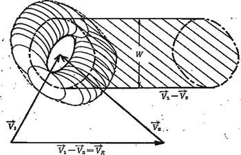
Fujii et al. (Reference Fujii, Yamanouchi and Mizuki1974) developed a method to estimate the number of Ship_2s in the area where collisions with a Ship_1 occur. This is the hatched area in Figure 1. The shape of each ship is approximated as an ellipse. The important value is the collision diameter (W) in Figure 1. Ship_2s that collide with a Ship_1 have a relative velocity $\overrightarrow {{V_2}} - \overrightarrow {{V_1}}$ . The number of Ship_2s that collide with a Ship_1 in a unit time can be obtained by multiplying the hatched area of Figure 1 by the density of Ship_2s. The value of the shaded area can be obtained by adding $W \cdot |{\overrightarrow {{V_2}} - \overrightarrow {{V_1}} } |$
 to the area made by sliding Ship_2 around Ship_1.
Fujii's method for counting the number of ships potentially colliding with Ship_1

This method is regarded as the basis for the geometric estimation of ${N_{a }}$ . However, Fujii did not present an analytical form of W. Further, he did not include the number of Ship_2s in the area created by graphically sliding Ship_2 around Ship_1. This area is called CP, which is mentioned in the nomenclature and is explained in Section 3.
2.2 Pedersen's method
Based on Fujii's method, Pedersen (Reference Pedersen1995, Reference Pedersen2010) developed the analytical solution (Equation (2.1)) for ${D_{\text{COL}}}$ using a rectangle to represent the shape of a ship. This was the first occurrence of rectangle approximation.

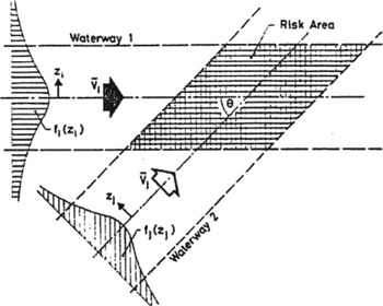
Pedersen's method obtained the number of collision candidates $({N_{CC}})$ in the intersection area of two waterways. This is schematised as a risk area in Figure 2, using the collision diameter. Equation (2.2) is supplemented with $1/\sin (\theta )$
 , which was not included in the original formulation. This sinusoidal form first appeared in Friis-Hansen (Reference Friis-Hansen2008). The variables in Equation (2.2) include suffixes i and j. These suffixes denote that there are groups of ships with the same characteristics, such as velocity and ship size. The suffixes i and j also denote the i-th and j-th groups of Ship_1s and Ship_2s, respectively.

Definition of the intersection area of two waterways (Pedersen, Reference Pedersen1995)

Some variables in Equation (2.2), which are not included in the nomenclature of this study, have the following meanings:
${N_{CC}}$
: Number of collision candidates in the intersectional area of waterways 1 and 2.V 1i: Velocity of ships in the i-th group of Ship_1.
V 2j: Velocity of ships in j-th group of Ship_2.
Q 1i: Mean appearance ratio of ships in the i-th group of Ship_1.
Q 2j: Mean appearance ratio of ships in the j-th group of Ship_2.
${D_{\text{COL} - ij}}$
: Collision diameter between a ship in the i-th group of Ship_1 and a ship in the j-th group of Ship_2.Vij: Relative velocity of a ship in the j-th group of Ship_2 as seen from a Ship_1 in group i.
$z_{i - \text{max}}^{(1 )}$
: The right-most appearance position of Ship_1 in the i-th group in waterway 1.$z_{i - \text{min}}^{(1 )}$
: The left-most appearance position of Ship_1 in the i-th group in waterway 1.$z_{j - \text{max}}^{(2 )}$
: The right-most appearance position of Ship_2 in the j-th group in waterway 2.$z_{j - \text{min}}^{(2 )}$
: The left-most appearance position of Ship_2 in the j-th group at the end of waterway 2.$f_i^{(1 )}$
: Probabilistic distribution function of the appearance position of Ship_1 in group i in waterway 1.$f_j^{(2 )}$
: Probabilistic distribution function of the appearance position of Ship_2 in group j in waterway 2.Δt: Considered time.


It is assumed that Δt is sufficiently longer than the time it takes for ships in waterways 1 and 2 to pass through the intersection. When the intersection angles are 0° and 180°, Equation (2.2) diverges, and therefore, different treatments are required. In these cases, ${N_{CC}}$ can be obtained using Equation (2.3):

where
$B_i^{(1 )}$
: Breadth of Ship_1 in group i.$B_j^{(2 )}$
: Breadth of Ship_2 in group j.$z_i^{(1 )}$
: Lateral position of Ship_1 in group i.$z_j^{(2 )}$
: Lateral position of Ship_2 in group j.


If $f_i^{(1 )}$ and $f_j^{(2 )}$
 are assumed to be probabilistic distribution functions of normal distribution, then Equation (2.3) can be approximated by Equation (2.4).

where
$\mu _i^{(1 )}$
: Mean value of the horizontal coordinate of the appearance position of a ship in the i-th group of Ship_1s.$\mu _j^{(2 )}$
: Mean value of the horizontal coordinate of the appearance position of a ship in the j-th group of Ship_2s.$\sigma _i^{(1 )}$
: Standard deviation of the horizontal coordinate of the appearance position of a ship in the i-th group of Ship_1s.$\sigma _j^{(2 )}$
: Standard deviation of the horizontal coordinate of the appearance position of a ship in the j-th group of Ship_2s.
\[|{V_i^{(1 )} \pm V_j^{(2 )}} |= \left\{ {\begin{array}{*{20}{c}} {V_i^{(1 )} + V_j^{(2 )};\theta = 180\;\text{deg}}\\ {|{\; V_i^{(1 )} - V_j^{(2 )}} |;\theta = 0\; \;\text{deg}} \end{array}} \right.\]



2.3 COWI's method
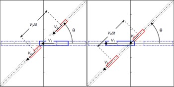
Both Fujii and Pedersen represented the collision of Ship_2s with a Ship_1 in a coordinate system fixed to the Ship_1 and modelled the collision, whereas the method devised by COWI engineering consultants (COWI, 2008) used a space fixed coordinate system. As shown in Figure 3, ships in the diagonal narrow waterway, whose breadth is the same as the breadth of a Ship_2, will collide with Ship_1s that travel from right to left. Here, the intersection angle between waterways 1 and 2 is expressed as $\; \theta$ . The diagram on the left-hand side of Figure 3 is the earliest situation for a Ship_1 to collide with a Ship_2, and the diagram on the right-hand side is the latest. Assuming that the time difference between the two situations is Δt and the mean appearance ratio of Ship_2 is ${Q_2}$
 , then the number of Ship_2 s that collide with Ship_1 can be obtained by Equation (2.5). For the same reason that Pedersen's formulation cannot be used when $\theta$
 is 0° or 180°, Equation (2.5) cannot be used.
Representation made by COWI (2008) of collision between a Ship_1 and Ship_2 using a space fixed coordinate system

The COWI's formulation appears to be different from Pedersen's formulation. However, these two formulations produced the same results. Therefore, in Section 6, where the comparison with the other methods is shown, only Pedersen's method is used.

2.4 Kaneko's methods
2.4.1 First method
Kaneko (Reference Kaneko2002) developed a method for calculating ${N_{CC}}$ when a Ship_2 appeared on the border of a circular area representing the Poisson distribution and travelled inside the area at optional progress direction and a same velocity while a Ship_1 travelled toward the centre of the area (Figure 4). ${N_{CC}}$
 for Ship_1 is obtained using Equation (2.6).

where
V: Velocity of Ship_2 which appears on the border of the circular area.
r: Radius of a circle which approximates the shape of Ship_1 and of Ship_2.
ρ: Density of Ship_2s.
α: Ratio of V to the velocity of Ship_1.
T: Considered time.
E(x): Complete elliptic integral of the second kind of x.
The hatched area is where Ship_2 in the hatched area will collide with a Ship_1 at the center of the circular area (Kaneko, Reference Kaneko2002)

Kaneko (Reference Kaneko2002) also developed a method for the case of a rectangular area.
2.4.2 Second method
Kaneko (Reference Kaneko2013) developed a method for calculating ${N_{CC}}$ for ships approximated as rectangular, and where the intersection angle of two waterways is small. For these conditions, collision situations were divided into six cases, and a method was developed to characterise each case. At some intersection angles strong correlation was found between analytical and simulated results. Since its improvement is shown in this paper, other points are omitted.
3. Proposed new formulation
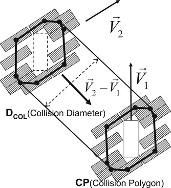
First, the shape of a ship is approximated as a rectangle. The figure of the centre point of Ship_2, which is made by sliding Ship_2 around Ship_1 keeping its heading angle, is called the collision polygon (CP) (Figure 5). CP is an octagon, and its area is calculated using Equation (3.1).

Collision situation in case of rectangular ships

As shown in Figure 6, the Ship_2s that are in a collision relationship while Ship_1s sail for time T have a relative velocity of $\overrightarrow {{V_2}} - \overrightarrow {{V_1}}$ and are located in a decagon. The longer parallel sides have a length of $|{\overrightarrow {{V_2}} - \overrightarrow {{V_1}} } |T$
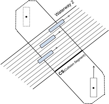
 . This figure is referred to as the collision area (CA). The line segment in a Ship_2's route made by being cut by CA was called collision segment (CS) (Figure 7). ${N_{CC}}$
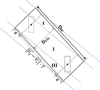
 was obtained by integrating the number of Ship_2 s in the CS. If Ship_1 completely passed through the intersection area between waterways 1 and 2, then the CS was included only in the parallel part of the CA. However, if Ship_1 did not completely pass through the intersection area during the consideration time because the width of waterway 2 is wide, the CS was integrated beyond the parallel part of the CA. Because a decagonal CA is complicated, CA is approximated as rectangular (Figure 8). The areas of both ends made after this simplification should be the same as the original CP, the area of which is obtained by Equation (3.1).
Collision area (CA)

Collision segment (CS)

Simplification of CA

The progress direction of Ship_2, $\theta$ , was measured clockwise from the negative progress direction of Ship_1. When the progress direction of Ship_2 is head-on to a Ship_1, $\theta$
 is 0°, and when the progress direction of Ship_2 is the same as Ship_1, $\theta$
 is 180°. Then, the angle of the relative velocity of Ship_2 measured from the negative progress direction of Ship_1 $({\theta _{\overrightarrow {{V_2}} \cdot \overrightarrow {{V_2}} - \overrightarrow {{V_1}} }})$
 , satisfies $0 \le {\theta _{\overrightarrow {{V_2}} \cdot \overrightarrow {{V_2}} - \overrightarrow {{V_1}} }} \le \theta$
 .
Therefore, the range of ${\theta _{\overrightarrow {{V_2}} \cdot \overrightarrow {{V_2}} - \overrightarrow {{V_1}} }}$ becomes wider as θ approaches 180°.
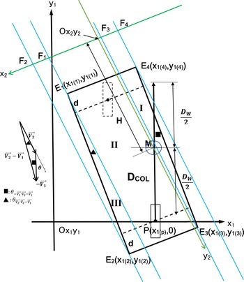
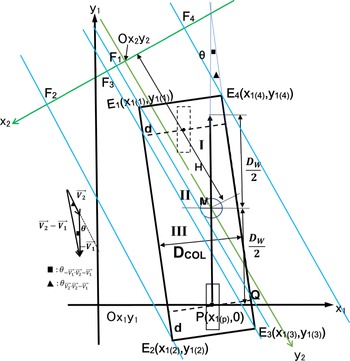
The number of Ship_2s that may collide with Ship_1 during the travel time of Ship_1 was obtained by integrating the number of Ship_2s in the CS in Figure 7 over the CA. From the geometric point of view, the essential relationship between the CA and the intersection angle (the progress direction of Ship_2) should be limited to the two cases illustrated in Figures 9 and 10. These two cases correspond to how CA is divided into three areas using four straight lines that pass through four vertices of CA and are parallel to waterway 2. The cases are explained as follows:
Relation between CS and CA in Case 1

Relation between CS and CA in Case 2

3.1 Case 1: ${D_{\textit{WL}}}\tan ({{\theta_{\overrightarrow {{V_2}} \cdot \overrightarrow {{V_2}} - \overrightarrow {{V_1}} }}} )< {D_{\rm{COL}}}$

Figure 9 shows three regions made by dividing CA by the longest CS, which passes through one of vertices and the shorter side of CA, and has a length of ${D_{\text{COL}}}$ . This case is likely to occur when the intersection angle is small, such that $\theta$
 is close or equal to 0° (head-on) or 180° (same direction). It also tends to occur when the velocity of Ship_1 is close to zero. Friis-Hansen (Reference Friis-Hansen2008) suggests that Pedersen's equation should be used only in the range of intersection angles between 10° and 170°. In this case, the value of Pedersen's equation becomes very large. In Pedersen (Reference Pedersen1995), ${N_{CC}}$
 is calculated using Equation (2.4) when the intersection angles are 0° and 180°. Until now, intersection angles outside the range of 10° to 170° have not been considered, except in the case of 0° and 180°, but the solution was obtained by the method described by Kaneko (Reference Kaneko2013). In this case, regions I and III in Figure 9 cannot be ignored. When ${\theta _{\overrightarrow {{V_2}} \cdot \overrightarrow {{V_2}} - \overrightarrow {{V_1}} }} = 0$
 , $\cos ({{\theta_{\overrightarrow {{V_2}} \cdot \overrightarrow {{V_2}} - \overrightarrow {{V_1}} }}} )= 1$
 not zero. In addition, if $\tan ({{\theta_{\overrightarrow {{V_2}} \cdot \overrightarrow {{V_2}} - \overrightarrow {{V_1}} }}} )< {D_{\text{COL}}}$
 , then ${\theta _{\overrightarrow {{V_2}} \cdot \overrightarrow {{V_2}} - \overrightarrow {{V_1}} }}$
 is not 90°. Therefore, ${N_{CC}}$
 can be determined using the method introduced in Section 4.
3.2 Case 2: ${D_{\textit{WL}}}\tan ({{\theta_{\overrightarrow {{V_2}} \cdot \overrightarrow {{V_2}} - \overrightarrow {{V_1}} }}} )\ge {D_{\rm{COL}}}$

Figure 10 shows three regions made by dividing CA with the longest CS, which passes through one of the vertices and the longer side of CA, and has a length of DWL. In this case, $\tan ({{\theta_{\overrightarrow {{V_2}} \cdot \overrightarrow {{V_2}} - \overrightarrow {{V_1}} }}} )$ does not become zero, that is, $\sin ({{\theta_{\overrightarrow {{V_2}} \cdot \overrightarrow {{V_2}} - \overrightarrow {{V_1}} }}} )$
 does not become 0, and ${\theta _{\overrightarrow {{V_2}} \cdot \overrightarrow {{V_2}} - \overrightarrow {{V_1}} }} \le \theta$
 , therefore $\sin (\theta )$
 does not become 0, and Pedersen's method can be used in this case. If the length of the longer side of the CA is longer than the width of waterway 2, that is, if Ship_1 completely passes through the intersection area, the integration of CS is necessary only in region II (Figure 10). Thus far, discussions on how to obtain ${N_{CC}}$
 have mainly focused on region II. However, if the width of waterway 2 is wide or Ship_1 stops in the intersection area, it is necessary to consider regions I and III.
4. A Method of Solution
Figures 11 and 12 illustrate the coordinate system used in this study. The line at the end of waterway 1, where Ship_1 appears, was defined as the horizontal axis (x 1-axis), and the course line of Ship_1 was defined as the vertical axis (y 1-axis). The origin was set at a suitable point on the horizontal axis. It was assumed that the centreline of waterway 2 passes through point M, which is located on the centreline of waterway 1, and the distance between M and x 1-axis is half of the sailing distance of Ship_1, that is, DW. The line at the end of waterway 2 where a Ship_2 appears is defined as another horizontal axis (x 2-axis), and the centreline of waterway 2 is defined as the corresponding vertical axis (y 2-axis). Further, the origin of the x 2–y 2 coordinate system is Ox 2y 2, and the distance of Ox 2y 2M is H. The location of Ship_1 is P, the coordinate of which is (X 1,0). CA is the rectangle E 1E 2E 3E 4, and the points projected on the x 2-axis of E 1, E 2, E 3, and E 4 are F 1, F 2, F 3, and F 4 respectively.
Coordinate system and related variables in Case 1

Coordinate system and related variables in Case 2

4.1 Case 1
Based on Figure 11, the estimation of ${N_{CC}}$ in this case is calculated as follows. Assuming the intersection of the line segments E 1F 3 and E 1E 4 of the CA is Q, the length ${L_{\text{Q}{\text{E}_\text{3}}}}$
 of the line segment QE3 can be obtained by Equation (4.1).

In case V 2 is constant, the number of Ship_2s that collide with Ship_1 while Ship_1 is navigating the distance DW can be obtained by integrating the quotient of CS in regions I, II, and III divided by Ship_2's velocity (V 2), with x 2.
${N_{CC}}$ in region I, ${N_{CC}}(\text{I})$
 , was calculated using Equation (4.2).

In the same manner, ${N_{CC}}$ in regions II and III, that is, ${N_{CC}}$
 (II) and ${N_{CC}}$
 (III), is determined in Equations (4.3) and (4.4), respectively.


The sum of the results is the total ${N_{CC}}$ s (N CC(I, II, III)) resulting from one Ship_1 travelling the distance DW when Ship_1s and Ship_2s have the same constant velocity, length, and breadth respectively. Moreover, by integrating ${N_{CC}}$
 (I, II, III) over the entire waterway 1 for a certain time (T), the number of collision candidates that are caused by Ship_1s and Ship_2s with the same constant velocity, ship length, and breadth respectively, while travelling for the duration (T), can be obtained. Furthermore, when the velocity, ship length, and breadth of Ship_1 and Ship_2 are probabilistically distributed, ${N_{CC}}$
 can be obtained by integrating them with these random variables as in Equation (4.5).

Equation (4.5) becomes Equation (4.6) if the variables, except for the appearance position, are constant.

When the intersection angle is 0° or 180°, Equation (4.7) is obtained.

Comparing Equation (4.7) with Equation (2.3) for the case where the intersection angle is 0° or 180° by Pedersen's method, Equation (4.7) contains the term $2T{Q_1}{Q_2}d/{V_2}$ which is not included in Equation (2.3). This shows that ${N_{CC}}$
 at both ends of the CA is included in Equation (4.7), which shows that the method developed here is more accurate than Pedersen's method.
4.2 Case 2
Based on Figure 12, the estimation of ${N_{CC}}$ in this case is calculated as follows. First, let the intersection of the line segments E 1F 3 and E 1E 4 of CA be Q, then the length ${L_{\text{Q}{\text{E}_\text{3}}}}$
 of the line segment QE3 can be obtained by Equation (4.8). The length of CS in region II is constant.

Therefore, ${N_{CC}}$ of Ship_1 with Ship_2s in regions I, II, and III are calculated using Equations (4.9)–(4.11), respectively.


In Case 2, $\sin ({{\theta_{\overrightarrow {{V_2}} \cdot \overrightarrow {{V_2}} - \overrightarrow {{V_1}} }}} )\;$ does not become zero, so a solution always exists.
Furthermore, when all the variables concerned are random variables, the expected value of the total number of collision candidates $({N_{CC}}({Q_1},{Q_2},{V_1},{V_2},{L_1},{L_2},{B_1},{B_2}))$ in the duration (T) is calculated using Equation (4.12).

Equation (4.12) becomes Equation (4.13) if the variables, except for the position of occurrence, are constant.

If Ship_1 completely passes through the intersection, that is, if the width of waterway 2 is completely included in Ship_1's CA, Equation (4.13) becomes Equation (4.14), which is the same as the equation by Pedersen (Equation (2.2)).

5. Validation by Simulation
The modelling explained in Sections 3 and 4 was closely realised by the program in which ships travelling in waterways 1 and 2 were made to appear, and many simulations were carried out to obtain ${N_{CC}}$ using the coordinate system presented in Section 4.
All Ship_1s travelling in waterway 1 appeared at (500,0) at a rate of 60 ships per hour, according to the Poisson distribution, and went straight along the y 1-axis at a constant velocity. Ship_2s appeared on the x 2-axis, according to a normal distribution, with a mean value of zero and a standard deviation of 150 m, while travelling in parallel with the y 2-axis. The appearance ratio of Ship_2s was 120 ships per hour, appearing according to the Poisson distribution. Simulations were carried out at each intersection angle until ${N_{CC}}$ obtained for Ship_1 entered the confidence interval. Table 1 lists the conditions of the simulation.
Simulation conditions

To predict a collision, after Ship_2 appeared, the distance to the closest point of approach was calculated for every Ship_1. For values less than or equal to half of ${D_{\text{COL}}}$ , the time to the closest point of approach (TCPA) was calculated. When TCPA was shorter than 30 s, Ship_2 was considered a collision ship.
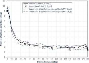
Simulations were performed at every predetermined intersection angle of 0° to 180° for cases in which the velocity of every Ship_2 was constant, and for the cases in which velocity was distributed according to the normal distribution of the predetermined mean value and the standard deviation of 2 m/s. The results are shown in Figures 12 and 13, respectively. Because the number of ship collisions is a Poisson distribution, the confidence interval of ${N_{CC}}$ per ship can be obtained by Equation (5.1). The risk rate was estimated to be 5% on both sides.

where
N: Number of collision candidates in simulations
M: Number of Ship_1s that appeared in the simulations
${\chi ^2}({\alpha ,F} )$
: The value of a random variable of the Chi squared distribution when the degrees of freedom value is F and the cumulative distribution function is α.

Collision simulation results (Velocity is constant)

Collision simulation results (with velocity distribution, standard deviation = 2 m/sec)

Table 1 shows conditions used in the simulations.
Figure 13 shows the results when the velocity of a Ship_2 is constant at 15 knots, and Figure 14 shows the results when the velocity of a Ship_2 had a normal distribution with a mean value of 15 knots and a standard deviation of 2 m/s.
From Figures 13 and 14, the average value of ${N_{CC}}$ per Ship_1 based on the simulation results is close to the value obtained by the method explained in Section 4, regardless of the presence of velocity distribution, and is located within the confidence interval of 5% risk for both sides at all considered intersection angles. Therefore, it is concluded that the proposed method was statistically validated.
At least two studies have estimated ${N_{CC}}$ by computer simulation (Friis-Hansen, Reference Friis-Hansen2008; Lušić and Čorić, Reference Lušić and Čorić2015). These results agree well with the analytical values reported by Pedersen. In particular, in Friis-Hansen (Reference Friis-Hansen2008), a simulation was carried out by generating ships, according to a Poisson distribution, assuming a traffic volume of 40 years, and compared with Pedersen's equation (Equation (2.2)). The two agree, however, their results have not yet been validated statistically. This paper is probably the first to report validated simulations at intersection angles of less than 10°, and 170° or more, excepting 0° and 180°.
6. Comparison with Pedersen's Methods
The method used in this study was compared with that of Pedersen. The results are shown in Figure 15. In the absence of velocity distribution, the solutions of this and Pedersen's method are in good agreement. However, at intersection angles less than 10° and larger than 170°, they diverge. The method developed here produces accurate values at all intersection angles.
Comparison of the number of collision candidates estimated by the methods of Pedersen and of Kaneko

When the intersection angles were 0° and 180°, Pedersen's values were calculated using Equation (2.4), when the standard deviation of Ship_1's appearance position was zero. The values estimated by this method at intersection angles of 0° and 180° were slightly larger than those estimated by Pedersen's method, but are closer to the simulation results. In this comparison, the same conditions were used that were used in Section 5.
7. Discussion
From a geometric perspective, it became clear that there are essentially only two types of intersections to be considered when estimating ${N_{CC}}$ in the intersection area of two waterways, regardless of the angle of intersection. The angle between the ships’ velocity vectors and the intersection angle between waterways are important. Case 1 occurs when this angle is small enough for the longest CS to intersect only the short sides of the CA. When this angle is large enough for the longest CS to intersect the short and long sides of the CA, Case 2 will occur. As Equation (4.5) indicates, in Case 1, the cosine of the angle between the relative velocity between ships and the intersection angle between waterways appears in the denominator, but as Equation (4.13) indicates in Case 2, the sine of the angle appears, and they are not zero. Therefore, the applicability of this method does not depend on the intersection angle of the waterways and can be used at all intersection angles. Until now, the Pedersen and COWI equations have been used only for the intersection angles from 10° to 170°, but in the future, the method developed here can be used regardless of the intersection angle.
In addition, it was clarified that the geometric estimation of ${N_{CC}}$ , so far, is only in the case where a collided ship travels a sufficient amount of time and can completely pass the intersection; that is, only when the waterway of a colliding ship is included in region II of CA in Case 2, as explained in Section 4.2. Case 1 had not been considered prior to the work of Kaneko (Reference Kaneko2013). Furthermore, even in Case 2, regions I and III should be considered to estimate ${N_{CC}}$
 accurately when Ship_1 does not completely pass through the intersection area. This study provides a method for estimating ${N_{CC}}$
 at the intersection of two waterways at all intersection angles. However, this is only true when the ship is assumed to be rectangular. In addition, if the ship is considered to be rectangular, the accurate shape of the CA is decagonal, which we approximate as a rectangle with a constant area. This simplification of CA is accurate when the intersection angles are 0° and 180°. Furthermore, if the mean number of appearance ships per unit length on the CS is the same in any part of the CA, meaning that the number of ships appearing per unit time is the same in any part of the appearance end of the waterway, this method can provide an accurate value.
If ships travel for a sufficient time and all collided ships pass through the intersection, ${N_{CC}}$ does not depend on the ship appearance distribution and is proportional to the number of ship appearances per unit time. However, if the appearance distribution of the colliding ship is wide, or if there are few Ship_1s passing through the intersection, Pedersen's method, which does not consider this, becomes inaccurate. Moreover, from Figures 13 and 14, it was confirmed that ${N_{CC}}$
 is larger when there are velocity distributions. In the case of overtaking (the intersection angle is 180°), ${N_{CC}}$
 becomes zero in Pedersen's equation (Equation (2.4)). However, if there is a velocity distribution, ${N_{CC}}$
 is greater than zero, and the method proposed in this paper can accurately estimate ${N_{CC}}$
 .
This method has some uncertainty in that, by assuming that the shape of the ship is rectangular and simplifying CA to rectangular, there are subtle differences between the results when the actual shape of ships and CA are used. The quantitative differences have not yet been evaluated. However, in the case of Ship_1's complete passage through the intersection area, the simplification of CA is not a problem. There is a difference if the passage of Ship_1 is not completed. However, for intersection angles of 0° and 180°, the results in the simplified CA are the same as those of the actual CA. It seems that the difference at other small intersections is insignificant, but further evaluation is necessary. Furthermore, this method cannot estimate ${N_{CC}}$ with anchored ships.
8. Conclusion
The main conclusions are summarised in the following:
(1) In this study, a method for estimating ${N_{CC}}$
at all intersection angles between two waterways was developed. It is now possible to estimate ${N_{CC}}$ accurately in the intersection area at all intersection angles, including a small angle that is less than 10° or more than 170°. In addition, by using an Excel table in which the VBS program is embedded, it has become possible to obtain ${N_{CC}}$ in the intersection area easily at any intersection angle.(2) When calculating ${N_{CC}}$
, it was found that it is necessary to consider two cases separately for CA and CS. Furthermore, in each case, it is necessary to divide CA into three regions according to the change in the length of CS.(3) This method was compared with Pedersen's method, and it was confirmed that these two methods can produce almost the same value for the range of 10° to 170°, and at 0° and 180°. This means that the more rational method developed here validated Pedersen's method. Therefore, there is no problem in using Pedersen's method for these intersection angles. However, even with Pedersen's method, it is necessary to perform numerical integration to consider the velocity and size distributions of the ships. Therefore, an Excel table with the VBL program embedded to integrate the position and velocity probability distribution functions is useful.
(4) The results of this method were compared with the simulation results. It was confirmed that at all intersection angles considered here, the results of this method were within the confidence interval, derived from simulation results, of 5% risk for both sides. From this, we conclude that this method is statistically validated.


Conflict of interest
The authors declare that there are no conflicts of interest regarding the publication of this paper.