


INTRODUCTION
Rigorous exploration of causal effects has become a key part of social science inquiry. No longer is it sufficient for researchers to claim a causal finding without additional theorizing and evidence of how the effect came to be. For many scholars, these inquiries usually involve ruling out different possible explanations. For example, does colonial status affect development even among countries with similar kinds of institutions? Does the incumbency advantage in American politics operate even when challengers are of comparable quality? Does a country’s natural resource wealth affect democracy even among countries with identical levels of state repression? These important debates illustrate that disparate literatures share a similar concern: does a causal finding remain even after controlling for factors that are realized after, and possibly due to, the treatment in question?
An extremely common approach to these types of questions is to simply condition on (or “control for”) posttreatment variables—i.e., variables on the causal path leading from the treatment of interest to the dependent variable. The goal here, implicitly or explicitly, is for authors to produce a causal effect estimate washed of an alternative explanation. As an illustration of just how widespread this approach is, we reviewed all empirical papers published in three of the top journals in political science from 2010 to 2015.Footnote 1 Of these papers, 40% explicitly conditioned on a posttreatment variable in the analysis; an additional 27% conditioned on a variable that could plausibly be posttreatment.Footnote 2 (Only 33% of the papers clearly had no posttreatment variables included in their analyses.) Thus, we estimate that as many as two-thirds of empirical papers in political science that make causal claims condition on posttreatment variables. This is a figure that includes both observational and experimental studies (see Figure 1). Furthermore, when we reviewed why these variables were used, we discovered that about 23% of the papers that condition on posttreatment variables did so in order to explicitly test or adjudicate between causal mechanisms, with the rest attempting to control for alternative causal pathways. In short, this analysis suggests that a majority of empirical articles in political science are attempting to estimate the direct effect of a treatment fixing some consequences of that treatment.
Proportion of Papers Implicitly or Explicitly Estimating Causal Relationships that include a Posttreatment Variable

Unfortunately, however, simply conditioning on posttreatment variables can result in seriously biased estimates of these direct effects. The key contribution of this article is to show that researchers can still estimate direct effects free of bias in a wide variety of empirical settings. To do so, we focus on a simple quantity of interest: the controlled direct effect (CDE). The CDE represents the causal effect of a treatment when the mediator is fixed at a particular level. This allows researchers to rule out whether rival explanations or theories are the exclusive drivers of their findings, which, as our analysis of recent articles shows, is an important goal for many political scientists. In addition, the CDE is the quantity of interest identified from an experimental design where both the treatment and mediator are set to particular levels. Designs of this variety, such as traditional factorial designs and conjoint analyses, are playing an increasingly important role in our understanding of politics. While this makes the CDE well suited to answering policy and program evaluation questions, we show below that it can also speak to causal mechanisms under certain assumptions. Thus, the CDE is an important part of the applied researcher’s causal toolkit.
A problem associated with the estimation of direct effects, controlled or otherwise, is what we call intermediate variable bias, which is attributable to intermediate confounders—or variables that are affected by the treatment and affect both the mediator and outcome. To estimate the controlled direct effect without such bias, we introduce a method from the biostatistics literature that addresses these challenges and is well suited for continuous treatments and mediators. The method is implemented by way of a simple two-stage regression estimator, the sequential g -estimator (Joffe and Greene Reference Joffe and Greene2009; Vansteelandt Reference Vansteelandt2009). This approach transforms (or demediates) the dependent variable by removing from it the effect of the mediator and then estimating the effect of the treatment on this demediated outcome. Under certain assumptions, it has been shown that this is a consistent estimate of the controlled direct effect. We extend the usefulness of this approach by deriving a consistent variance estimator and describing how to conduct a sensitivity analysis for the key identification assumption. The methodology is easy to use, intuitive, and straightforward to implement with existing statistical software. We also provide open-source software that implements these methods and calculates the correct variance estimates and conducts sensitivity analyses.
We note that the direct effect is part of a growing family of causal quantities that center on questions of direct and indirect effects. Another quantity, the natural direct effect (NDE), has been widely studied in both statistics (Pearl Reference Pearl2001) and political science (Imai et al. Reference Imai, Keele, Tingley and Yamamoto2011). The CDE and the NDE answer similar yet distinct causal questions and each has different properties. For instance, the total causal effect (the average treatment effect) can be decomposed into two quantities: the natural indirect effect and the natural direct effect, making the NDE useful for evaluating causal mechanisms. As we show below the decomposition of the total effect using the controlled direct effect is more complicated. Below we discuss these differences and highlight how the CDE and NDE approaches complement one another, noting when each has advantages in applied work. Together, these quantities provide a robust way for researchers to investigate and explain their causal findings.
We proceed as follows. We first explain why conditioning on posttreatment variables—the approach taken by many social scientists—has the potential to introduce serious bias. Next, we explain direct effects and controlled direct effects, showing how the latter speak to causal mechanisms. We then address the problems that result from the inclusion of intermediate confounders and then continue on to present sequential g-estimation (with our sensitivity analysis). The next section illustrates both the framework and method via two empirical examples, which we use throughout for illustrative purposes. First, we replicate Fearon and Laitin (Reference Fearon and Laitin2003), to explore whether ethnic fractionalization affects civil war onset primarily via its impact on political instability. Using sequential g-estimation, we show that ethnic fractionalization has a separate effect on civil war onset that does not operate through political instability. Second, we replicate Alesina, Giuliano, and Nunn (Reference Alesina, Giuliano and Nunn2013), who show that historical plough use has an effect on modern-day female political participation. This effect exists only after conditioning on current-day income levels, which could introduce bias. We use sequential g-estimation to estimate the direct effect of the plough not through income, finding an effect that is even stronger than in their original analyses. We then address differences between the CDE and the NDE and briefly conclude with thoughts for future research. In the Appendix, we show how to implement this approach with a few lines of code, either in R or Stata.Footnote 3
WHY CONDITIONING ON POSTTREATMENT VARIABLES CAN INTRODUCE SERIOUS BIAS
As we discussed above, up to two-thirds of articles within political science appear to condition on posttreatment (or possibly posttreatment) variables. Unfortunately, this practice raises two potentially serious complications. First, conditioning on a posttreatment variable changes the quantity of interest from an overall average treatment effect to a direct effect of the treatment net the posttreatment variable. This change may be expected and may be the goal of these analyses—indeed, this is the quantity that we set out to estimate below—but it also might conflict with researchers’ substantive interpretations. Even more sinister is the second consequence of conditioning on posttreatment variables, which is selection bias that leaves the coefficient of interest without any causal interpretation. (This bias is part of what we call intermediate variable bias, below.) Selection bias of this kind occurs because the posttreatment variable could be endogenous and related to the outcome in noncausal ways. When this occurs, conditioning on this variable can induce spurious correlations between the treatment and the outcome (Rosenbaum Reference Rosenbaum1984).
A simple thought experiment helps to illustrate this form of selection bias. For many reasons, a reasonable assumption is that there exists no causal relationship between being in a car accident and having cancer; that is, being in a car accident does not plausibly lead someone to develop or be cured of cancer. However, if we were to condition on being a patient in a hospital (posttreatment to having been in a car accident), we would see a strong negative correlation between these two conditions: patients are admitted to the hospital for either condition, so that if a patient is in the hospital and has not been in a car accident, they must be sick or unwell in some other way, increasing the likelihood that the patient has cancer. Thus, conditioning on being in a hospital would induce a negative relationship between being in a car accident and having cancer. However, this relationship does not exist because car accidents have a strong cancer-fighting effect, but rather because conditioning on being in the hospital produces additional information and breaks the statistical independence between car accidents and cancer.
A simple simulation shows this more concretely. We base the simulation on the following:

The “mediator” is the posttreatment variable in question. Neither the treatment nor the mediator have an effect (direct or indirect) on the outcome. The mediator is correlated with the outcome through their common cause, labelled as the confounder. We generate data from this process and plot the relationship between the treatment and both the confounder and the outcome. Figure 2 shows the results of one such draw. Looking at the overall relationships, including the grey and black dots, we see, as expected, that there is no effect of treatment on the confounder or the outcome. When we condition on the mediator, however, we see a much different picture. The black dots in Figure 2 are observations that have a value of the mediator in a certain range. Here, conditioning on certain values of the mediator induces strong correlations between the treatment and (1) the confounder (left plot) and (2) the outcome (right plot), even though there is no effect of the treatment on either by construction. This is selection bias that is induced by conditioning on the mediator. Indeed, as the statistical literature has long pointed out, this bias need not be conservative—here we are inducing relationships where none exist. Of course, when using real data, we will have no idea as to the direction of such bias.
Simulated Data Showing the Problem with Conditioning on a Posttreatment Variable

What does this bias mean for the applied researcher? First, coefficients estimated from models that condition on posttreatment variables might not have a causal interpretation. Second, in some instances, the inclusion of posttreatment variables into a statistical analysis can bias the estimator away from zero, meaning that the estimates may overstate the size of a causal effect in either direction. Third, the bias means that any estimates may also be inconsistent: as sample sizes increase, the coefficients from models that include posttreatment variables will actually converge to the wrong quantity. Thus, from the perspective of applied researchers, the problems associated with conditioning on posttreatment variables can be extremely serious.
WHAT ARE DIRECT EFFECTS?
Given these problems, conditioning on posttreatment variables in a statistical model is seldom a suitable approach to causal inquiries. But how can researchers estimate direct effects without bias? In this section, we introduce a quantity of interest that fits the substantive goals of most researchers and can be estimated, free of bias, with a simple procedure. We start with the direct effect of a treatment, which is the effect of the treatment for a fixed value of the mediator (though how one “fixes” the mediator matters a great deal). Our goal in this article is to estimate the controlled direct effect (CDE) of the treatment, which is the direct effect of the treatment when a mediator is the same fixed value for all units.Footnote 4 An indirect effect, on the other hand, is the portion of the total effect of treatment due to the treatment’s effect on the mediator and the mediator’s subsequent effect on the outcome.
We illustrate these concepts via a recurring example from comparative politics: Does ethnic fractionalization affect the onset of civil wars (Fearon and Laitin Reference Fearon and Laitin2003)? Specifically, does ethnic fractionalization increase the probability that a country will have a civil war primarily because it leads to greater political instability? Or does ethnic fractionalization increase the probability of civil war onset independently of greater instability? Our question of interest is whether ethnic fractionalization continues to have an independent effect on civil war onset holding political instability fixed at some value for all countries.
Potential Outcomes
To develop the framework, we rely on the potential outcomes model of causal inference (Holland Reference Holland1986; Neyman Reference Neyman1923; Rubin Reference Rubin1974), a counterfactual-based framework (that we summarize only briefly here). The advantage here, in contrast to a more traditional structural equation modeling approach, is that the potential outcomes framework allows us to incorporate heterogeneous causal effects easily and decouples the definition of a causal effect from its estimation. Let Ai
be the treatment of interest, taking values
 $a \in \mathcal {A}$
, where
 $\mathcal {A}$
is the set of possible treatment values. We define Mi
as the mediator, taking values
 $m \in \mathcal {M}$
. Throughout the article, we assume both are continuous. Using our example, Ai
represents ethnic fractionalization in a given country, while Mi
represents the mediator, the country’s political instability.
Studies of direct effects generally involve two sets of covariates. The first, which we call pretreatment confounders (Xi ), are variables that affect the treatment, the outcome, and possibly the mediator. The second, which we call intermediate confounders (Zi ), are consequences of the treatment that also affect the mediator and outcome. These are intermediate because they causally come between the treatment and mediator, as shown in Figure 3. For example, a country’s average income is probably an intermediate confounder because it is (1) affected by ethnic fractionalization and (2) confounds the relationship between political instability and civil conflict. As we show below, such intermediate confounders cause major problems for the estimation of direct effects.
Directed Acyclic Graph Showing the Causal Relationships Present in Analyzing Causal Mechanisms

Total Effects
Let Yi be the observed outcome for unit i and Yi (a) be its potential outcome, the value that unit i would take if we set (and only set) the treatment to a. For instance, if the outcome was the country-level number of battle deaths due to civil conflict, then Yi (a) would be the number of battle deaths if ethnic fractionalization was set to a. The potential outcomes connect to the observed outcome by the consistency assumption, Yi = Yi (Ai ), under which we observe the potential outcome for the observed treatment level.
In the potential outcomes framework, a causal effect is the difference between two potential outcomes, τ i (a, a′) = Yi (a) − Yi (a′). This is the difference in outcomes if we were to switch unit i from treatment level a′ to a. Under the consistency assumption, we only observe one of these potential outcomes for any unit—a problem known as the “fundamental problem of causal inference.” To circumvent this, we typically estimate the average of treatment effects. We define the average treatment effect or average total effect (ATE, or τ) to be the difference in means between two different potential outcomes:
 $$\begin{equation}
ATE(a,a^{\prime }) = E[Y_i(a) - Y_i(a^{\prime })],
\end{equation}$$
where E[ · ] denotes the expectation over units in the population of interest. This is just the average effect if we were to change ethnic fractionalization from a′ to a in all countries.
Controlled Direct Effects
To define controlled direct effects, we imagine intervening on both the treatment and the mediator at once. We define Yi (a, m) to be the value that the outcome that unit i would take if we set its treatment to a and the mediator to m. For country-level number of battle deaths due to civil conflict, for example, Yi (a, m) would represent battle deaths if ethnic fractionalization was set to a and political instability to m. Under the same consistency assumption, then Yi = Yi (Ai , Mi ). The mediator also has potential values, Mi (a), defined similarly to the potential outcomes; that is, Mi (a) refers to the potential value that the mediator would take on under treatment level a. Applying the consistency assumption again, we have Mi = Mi (Ai ). Note that the potential outcome only setting a is the composition of these two potential outcomes: Yi (a) = Yi (a, Mi (a)).
The controlled direct effect (CDE) is the effect of changing the treatment while fixing the value of the mediator at some level m (Pearl Reference Pearl2001; Robins Reference Robins, Green, Hjort and Richardson2003):
 $$\begin{equation}
CDE_{i}(a,a^{\prime },m) = Y_i(a,m) - Y_i(a^{\prime },m).
\end{equation}$$
As with total effects, it is difficult to identify individual-level effects and so we focus on the average CDE or ACDE:
 $$\begin{equation}
ACDE(a,a^{\prime },m) = E[Y_i(a,m) - Y_i(a^{\prime },m)].
\end{equation}$$
In other words, while a direct effect in general fixes the value of the mediator, the ACDE more closely corresponds to a ceteris paribus definition of a direct effect—that is, it is the direct effect with the mediator fixed at some value for all units in the population. It is the effect of separately fixing Ai and Mi to particular values for all units. In our example, this quantity of interest represents the effect of changing ethnic fractionalization if we were to fix the amount of political instability in a country at some level. The controlled direct effect is what is implicitly or explicitly estimated in experiments where units are randomized to receive more than one treatment, a research design increasingly common in political science.
Natural Direct and Indirect Effects
We note other important estimands for direct effects (Pearl Reference Pearl2001; Robins and Greenland Reference Robins and Greenland1992), which are common in the causal mediation literature. One quantity of interest is the natural direct effect (NDE), which is the effect of changing treatment when fixing the mediator to its unit-specific potential value under a particular treatment level:
 $$\begin{equation}
NDE_i(a,a^{\prime }) = Y_i(a, M_i(a^{\prime })) - Y_i(a^{\prime }, M_i(a^{\prime })).
\end{equation}$$
The second value after the equality is simply the potential outcome Yi (a′) under the treatment level a′. The natural direct effect represents the effect of a modified treatment that does not affect the mediator, but continues to directly affect the outcome. In our example this would be the effect of moving from complete ethnic homogeneity to some value a of ethnic fractionalization, holding political instability at what it would be under ethnic homogeneity. Note the crucial difference between the CDE and the NDE is at what level one “fixes” the value of the mediator.
A related quantity of interest is the natural indirect effect (NIE), which fixes the treatment and quantifies how the outcome changes only in response to treatment-induced changes in the mediator:
 $$\begin{equation}
NIE_i(a,a^{\prime }) = Y_i(a, M_i(a)) - Y_i(a, M_i(a^{\prime })).
\end{equation}$$
The first term after the equality is, again, the potential outcome under a. The natural direct and indirect effect decompose the total effect for a single unit:
 $$\begin{equation}
\tau _i(a,a^{\prime }) = NIE_i(a,a^{\prime }) + NDE_i(a,a^{\prime }).
\end{equation}$$
This decomposition also holds when we replace the individual-level quantities with their averages, ATE(a, a′) = ANIE(a, a′) + ANDE(a, a′), where ANIE and ANDE are the averages of the NIE and NDE, respectively. We discuss the relative advantages of the ACDE and ANDE below.
How Controlled Direct Effects Speak to Causal Mechanisms
As we discuss below, the statistical literature on direct effects has mostly discussed the advantages of the ACDE in the context of experiments and policy evaluation. While these goals are very useful for scholars, in this section, we show how the ACDE can also speak to causal mechanisms in two distinct ways. Note that the ANDE is the more straightforward estimand for evaluating mechanisms, but as we discuss below, it is often not identified in applied settings, leaving ACDE as a scholar’s only option. Thus, the information that the ACDE can provide about mechanisms is important.
(1) Ruling out alternative mechanisms. First, as VanderWeele (Reference VanderWeele2011) notes, if the effect of a treatment is completely mediated by a mediator Mi and another set of potential mediators, Wi , then a nonzero ACDE for Mi implies that there must be an indirect effect that works through the set Wi .Footnote 5 Thus, showing that there is a nonzero ACDE implies that the effect of treatment is not due to the Mi mechanism exclusively. In the Appendix, we provide a formal proof of this result. For example, if our goal was to show that ethnic fractionalization had some effect on civil war deaths other than through political instability, we would estimate the ACDE and check its proximity to zero, taking into account uncertainty through a confidence interval or hypothesis test. A nonzero ACDE would suggest that there does exist an effect of ethnic fractionalization that does not operate exclusively through political instability. This is an intuitive approach for many applied researchers, who frequently want to rule out alternative explanations as being sole determinants of their findings.
(2) Support for a preferred mechanism. Second, the difference between the ATE and ACDE summarizes the role of the mediator in a causal mechanism for the effect of Ai , allowing us to estimate support for a preferred mechanism. To see this, decomposing the total effect into three components is useful. VanderWeele (Reference VanderWeele2014) and VanderWeele and Tchetgen Tchetgen (Reference VanderWeele and Tchetgen2014) show that, with a binary mediator Mi , we can decompose the overall effect into the following:Footnote 6
 $$\begin{eqnarray}
\tau (a,a^{\prime }) &=& \underbrace{ACDE(a,a^{\prime },0)}_{\text{direct effect}} + \underbrace{ANIE(a,a^{\prime })}_{\text{indirect effect}} \nonumber\\
&&+\, \underbrace{E\big [M_i(a^{\prime })[CDE_i(a,a^{\prime },1) {-} CDE_i(a,a^{\prime },0)]\big ]}_{\text{interaction effect}}{.}\nonumber\\
\end{eqnarray}$$
This decomposition shows that between the ATE and ACDE is a combination of (1) the average natural indirect effect and (2) an interaction effect that captures how much the direct effect of Ai depends (causally) on Mi at the individual level. (Note that this interaction effect is distinct from the more typical “effect modification,” which is a noncausal statement about how average effects vary as a function of potentially nonmanipulated variables.) Under the constant interactions assumption
 $$\begin{eqnarray}
CDE_i(a,a^{\prime },m) - CDE_i(a,a^{\prime },m^{\prime }) = d(m-m^{\prime }),
\end{eqnarray}$$
the interaction effect in (7) simplifies to d · E[Mi (a′)] (whether the mediator is binary or continuous) and is identified under our assumptions (stated formally below). Imai and Yamamoto (Reference Imai and Yamamoto2013) explored this assumption to compare the indirect effect of two competing mechanisms. This result also implies that we can recenter Mi such that E[Mi (a′)] = 0, and the total effect decomposes into the ACDE and the ANIE. Thus, under the constant interactions assumption and the identification assumptions below, the difference between the ATE and the ACDE is a measure of the indirect effect, provided we recenter Mi as M* i = Mi − E[Mi (a′)].
Without the constant interaction assumption, it will be infeasible to separate out the indirect effect from the interaction effect in (7). Even in this situation, the difference between the ATE and ACDE might still provide some information on how the causal finding came to be if we take a broader definition of causal mechanisms than is currently used in the statistics and biostatistics literature. Both the indirect effect and the interaction effect measure the impact of the mediator on how the treatment affects the outcome. The indirect effect measures how strong a particular causal pathway is, while the interaction effect tells us how much the mediator influences the direct effect of the treatment. The difference between the ATE and ACDE, then, will provide an aggregation of these two effects, which can be seen as a summary of how Mi participates in a causal mechanism for the effect of Ai on Yi . This definition of a causal mechanism, however, is more expansive than previous definitions. For example, Imai, Keele, and Yamamoto (Reference Imai, Keele and Yamamoto2010) defines a causal mechanisms in terms of indirect effects. Thus, the difference in their framework between the ATE and the ANDE is the relevant measure of the strength of a mechanism. Referencing (7), this is equivalent to combining the ACDE and the interaction effect to create the ANDE. VanderWeele (Reference VanderWeele2009), on the other hand, defines mechanisms in terms of the sufficient cause framework and shows that while there being an indirect effect through Mi implies that Mi participates in a mechanism, the reverse is not true. That is, there can be variables that participate in a mechanism that are unaffected by the treatment. For applied researchers, the empirical application will determine the utility of these approaches. In some cases, indirect effects are of particular interest while in others the combination of indirect effects and interaction is sufficient. We discuss these distinctions further below.
INTERMEDIATE VARIABLE BIAS
All direct effect quantities of interest—including both the ACDE and ANDE—raise the possibility of intermediate confounders. These intermediate confounders (Zi in Figure 3) in turn raise the possibility of intermediate variable bias, a type of posttreatment bias. The intuition is as follows: Conditioning on a mediator results in selection bias unless all of the intermediate confounders are included as well (sometimes called M bias), but including them means including posttreatment variables (posttreatment bias). For instance, a researcher studying whether ethnic fractionalization affects civil war net political instability should be concerned whether there exist variables—measured or unmeasured—that (1) are affected by ethnic fractionalization and also (2) affect political instability and civil war onset. Such variables are confounders for the mediator, but are also affected by treatment and thus are intermediate confounders. Unfortunately, dozens of such variables probably exist in our example—for example, religious fractionalization, average income, racism, and so on.
Most previous approaches to causal mediation confront this problem by assuming that no intermediate confounders exist. Unfortunately, this may be an unrealistic assumption for many researchers,Footnote 7 with the vast majority of mediators in the social sciences certainly violating this no intermediate confounders assumption. As Imai, Keele, and Yamamoto (Reference Imai, Keele and Yamamoto2010) point out, no intermediate confounders “is an important limitation since assuming the absence of post-treatment confounders may not be credible in many applied settings” (p. 55). Moreover, the ANDE and the ANIE are unidentified in the presence of intermediate confounders without strong individual-level homogeneity assumptions (as we discuss below). This makes these quantities of interest less attractive for many applied researchers.
The ACDE is, by contrast, identified in the face of intermediate confounders (also discussed below). Even so, the possible presence of intermediate confounders does raise the possibility of intermediate variable bias. To show this, we first assume a correctly specified linear model with constant treatment effects and no omitted variables for Ai . Under these assumptions, we can estimate the causal effect of Ai in a regression of the outcome on the treatment and the pretreatment confounders,
 $$\begin{equation}
Y_i = \beta _0 + \beta _1A_i + X_i^T\beta _2 + \varepsilon _{i},
\end{equation}$$
where β1 is the (total) effect of Ai on Yi . A common way to gauge the strength of some mechanism is to include a mediator, Mi , as an additional regressor in the model,
 $$\begin{equation}
Y_i = \skew3\widetilde{\beta }_0 + \skew3\widetilde{\beta }_1A_i + \skew3\widetilde{\beta }_2M_i + X_i^T\skew3\widetilde{\beta }_3 + \varepsilon _{i},
\end{equation}$$
and to interpret
 $\skew3\widetilde{\beta }_1$
as a direct effect. Unfortunately, this interpretation is only correct under the assumption of no intermediate confounders. When these confounders, Zi
, are present, then
 $\skew3\widetilde{\beta }_1$
will not equal the ACDE nor the ANDE, even under constant effects. This is because conditioning on a posttreatment variable can induce spurious relationships between the treatment and the intermediate confounders and, thus, the outcome (Rosenbaum Reference Rosenbaum1984).
In order to avoid this bias, we might decide to include the intermediate confounders in the regression:
 $$\begin{equation}
Y_i = \alpha _0 + \alpha _1A_i + \alpha _2M_i + X_i^T\alpha _3 + Z_i^T\alpha _4 + \varepsilon _{i}.
\end{equation}$$
Unfortunately, here too the coefficient on the treatment, α1, will not be equal to the ACDE. This is because conditioning on Zi blocks a possible causal pathway from A → Z → Y, which is part of the controlled direct effect. Thus, both omitting and conditioning on the intermediate confounders leads to a biased estimate of the ACDE.
SEQUENTIAL g-ESTIMATION
In this section, we present sequential g-estimation, a method for estimating controlled direct effects in the face of intermediate confounders. Described by Vansteelandt (Reference Vansteelandt2009) and Joffe and Greene (Reference Joffe and Greene2009), it is a type of structural nested mean model (Robins Reference Robins1986; Reference Robins1994; Reference Robins and Berkane1997) that is tailored to estimating direct effects.Footnote 8 We present (1) the assumptions that underlie this method, (2) basic identification results, (3) implementation details, and (4) an approach to sensitivity analysis.
Assumptions
As pointed out by Robins (Reference Robins and Berkane1997), the ACDE is nonparametrically identified under what we call sequential unconfoundedness.
Assumption 1 (Sequential Unconfoundedness)
 $$\begin{eqnarray}
\lbrace Y_i(a,m), M_i(a)\rbrace \perp \!\perp A_i | X_i = x,
\end{eqnarray}$$
 $$\begin{eqnarray}
Y_i(a,m) \perp \!\!\!\perp M_i | A_i = a, X_i = x, Z_i = z,
\end{eqnarray}$$
for all possible treatment values
 $a \in \mathcal {A}$
, mediator values
 $m \in \mathcal {M}$
, and covariate values
 $x \in \mathcal {X}$
and
 $z \in \mathcal {Z}$
. In addition, we assume for all the above values:
 $$\begin{eqnarray}
P(A_i = a | X_i = x) > 0,
\end{eqnarray}$$
 $$\begin{eqnarray}
P(M_i = m| A_i = a, X_i = x, Z_i = z) > 0.
\end{eqnarray}$$
This assumption represents two separate “no omitted variables” assumptions. First, no omitted variables for the effect of treatment on the outcome, conditional on the pretreatment confounders. Second, no omitted variables for the effect of the mediator on the outcome, conditional on the treatment, pretreatment confounders, and intermediate confounders. Thus, this represents a selection-on-the-observables assumption for each analysis. Because such assumptions can be unrealistic in observational studies, we show below how to weaken this assumption through a sensitivity analysis. Note that the pretreatment confounders can include pretreatment measurements of the intermediate confounders, which can add to the credibility of this assumption.
Figure 4 shows a situation where sequential unconfoundedness is violated. Here, dashed lines represent the effects of unmeasured confounders U i1 and U i2. In the Fearon and Laitin (Reference Fearon and Laitin2003) illustration below, U i1 represents the omitted variables for the effect of ethnic fractionalization on civil war onset and U i2 represents the omitted variables for the effect of political instability on civil war onset. Sequential unconfoundedness assumes that both paths Ai ← U i1 → Yi and Mi ← U i2 → Yi are absent, meaning that we have included enough variables in the pretreatment and intermediate covariates, Xi and Zi , so that no omitted variable bias would be present in separately estimating the effect of either political instability or ethnic fractionalization on civil war onset.
Directed Acyclic Graph Showing a Violation of Sequential Unconfoundedness

In short, if the assumptions hold to separately estimate the effects of Ai and Mi on Yi , then sequential unconfoundedness holds. Of course, this assumption might be violated if, for example, there are determinants of political instability and civil war onset that are not included in either Xi or Zi . Because of the crucial nature of this assumption and the difficulty of showing that it holds in observational data, below we discuss a sensitivity analysis for assessing how large deviations from this assumption have to be in order to change the results of a study. Below, we apply this sensitivity analysis to the example of political instability and civil war onset.
Sequential unconfoundedness is not sufficient to identify the ANDE, however. To do so requires a stronger version of this assumption that omits intermediate confounders entirely so that both U i2 and Zi must be absent from Figure 4 (Imai, Keele, and Yamamoto Reference Imai, Keele and Yamamoto2010). In addition, identifying the ANDE requires potential outcomes from different counterfactual worlds to be independent (Imai, Keele, and Yamamoto Reference Imai, Keele and Yamamoto2010) or for individual-level no- or constant-interaction assumptions (Imai and Yamamoto Reference Imai and Yamamoto2013; Robins Reference Robins, Green, Hjort and Richardson2003). Thus, one advantage of the ACDE is that it is identified under far weaker assumptions than the ANDE. Of course, the ANDE helps partition the total effect at a finer level and calculate the strength of a given causal pathway versus all other pathways. However, this additional information comes at the cost of these additional strong assumptions.
Even though ACDEs are identified under Assumption 1 the effects depend on the distribution of the intermediate confounders (Robins Reference Robins and Berkane1997). To implement the simplest version of sequential g-estimation, we need the effect of the mediator on the outcome to be independent of the intermediate confounders.
Assumption 2 (No Intermediate Interactions)
 $$\begin{eqnarray}
&&E[Y_i(a,m) - Y_i(a,m^{\prime }) | X_i = x, A_i = a, Z_i = z ] \nonumber\\
&&= E [Y_i(a,m) - Y_i(a,m^{\prime }) |X_i = x, A_i = a ],
\end{eqnarray}$$
for all values
 $a \in \mathcal {A}$
,
 $m, m^{\prime } \in \mathcal {M}$
,
 $z \in \mathcal {Z}$
, and
 $x \in \mathcal {X}$
.
This assumption has several notable features. First, this assumption is not required for the nonparametric identification of the ACDE. Nonparametric identification only relies on sequential unconfoundedness and this no intermediate interactions assumption only serves to make estimation simpler. In fact, we can relax this assumption to the extent that we are willing to model the distribution of Zi conditional on Ai and Xi . Second, even if this assumption is false, the estimated effects will be weighted averages of ACDEs within levels of the intermediate confounders (Vansteelandt and Joffe Reference Vansteelandt and Joffe2014, 718). Thus, this assumption is similar to omitting an interaction term from a regression model. Third, this assumption does not rule out important interactions between the treatment and the mediator (see, for example, (24) below) nor interactions with the baseline covariates. Finally, this assumption is weaker than other no interaction assumptions (see, e.g., Robins Reference Robins, Green, Hjort and Richardson2003) that restrict the controlled direct effect at the individual level or other assumptions that rule out intermediate confounders entirely.
Identification
In order to tune the estimator to estimating direct effects, it is useful to define the following function, which we call the demediation function Footnote 9 :
 $$\begin{eqnarray}
\gamma (a,m,x) = E[Y_i(a,m) - Y_i(a,0)|X_i = x]
\end{eqnarray}$$
This function is the effect of switching from some level of the mediator to 0 and does not depend on the value of the intermediate confounders due to Assumption 2. We call this the demediation function because when subtracted from the observed outcome, Yi − γ(Ai , Mi , Xi ), it removes the variation in the outcome due to the causal effect of the mediator:
 $$\begin{eqnarray}
&&E[Y_i - \gamma (a,M_i,x) |A_i = a, X_i = x] \nonumber\\
&&= E[Y_i(a,0) | X_i = x].
\end{eqnarray}$$
This property of the demediation function follows easily from Assumptions 1 and 2 (Robins Reference Robins1994; Vansteelandt Reference Vansteelandt2009). Based on this, the ACDE conditional on Xi ,
 $$\begin{equation*}
E[Y_i(a,0) - Y_i(0,0) | X_i = x],
\end{equation*}$$
is nonparametrically identified as difference in means of the demediated outcome:
 $$\begin{eqnarray}
&&E[Y_i - \gamma (a, M_i, x)|A_i = a, X_i = x]\nonumber\\
&&\quad - E[Y_i - \gamma (0, M_i, x)|A_i = 0, X_i = x].
\end{eqnarray}$$
The key intuition here is that after demediating the outcome, the remaining covariation with Ai is due to the direct effect of Ai .
Of course this result requires us to know the demediation function, which is unrealistic. Instead, we will almost always estimate it from data. Robins (Reference Robins1994) showed that, under sequential unconfoundedness, the causal difference γ is nonparametrically identified from the data and is equal to the difference-in-means estimator conditional on all the previous variables:
 $$\begin{eqnarray}
&&\widehat{\gamma }(a,m,x) = \widehat{E}[Y_i|A_i = a, M_i = m, X_i = x, Z_i = z]\nonumber\\
&&\quad - \widehat{E}[Y_i| A_i = a, M_i = 0, X_i = x, Z_i = z].
\end{eqnarray}$$
This follows from the simple fact that sequential unconfoundedness implies that the effect of the mediator on the outcome is identified. This part of sequential unconfoundedness is the usual selection on the observables assumption often invoked to identify an average treatment effect in either a regression or matching context. Furthermore, the identification of the ACDE as (19) holds when replacing γ with its estimate,
 $\widehat{\gamma }$
.
Implementation
When the treatment and mediator are binary or only take on a few values, nonparametric or semiparametric approaches exist to estimating the ACDE, reducing the need for parametric models (Robins, Hernán, and Brumback Reference Robins, Hernán and Brumback2000).Footnote 10 With a continuous treatment and a continuous mediator, nonparametric and semiparametric estimation of the difference-in-means in Equations (20) and (19) have poor properties, including instability and high variability (Vansteelandt Reference Vansteelandt2009). Sequential g-estimation brings in parametric models to help estimate ACDEs in this context.
Sequential g-estimation proceeds in two simple steps. First, we regress the outcome on the mediator, treatment, and covariates (pretreatment and intermediate) to get an estimate of the demediation function. Second, we use the first stage to demediate the outcome and run a regression of this demediated outcome on the treatment and the pretreatment covariates. The marginal effect of the treatment in this second stage regression will be the estimate of the ACDE. We describe these steps in further detail.
First stage
The first stage of sequential g-estimation involves estimating the effect of Mi on Yi , conditional on all other variables. The components of this model that involve Mi will be the parameterization of the demediation function, γ. For instance, we might use the following regression function:
 $$\begin{eqnarray}
&&E[Y_i|A_i, M_i, X_i, Z_i] \nonumber\\
&&\quad= \alpha _0 + \alpha _1A_i + \alpha _2M_i + X_i^T\alpha _3 + Z_i^T\alpha _4.
\end{eqnarray}$$
This parametric model implies a parametric model on the demediation function, which is
 $$\begin{equation}
\gamma (a,m,x;\alpha ) = \gamma (m;\alpha _2) = \alpha _2m.
\end{equation}$$
We could augment this baseline regression model with interactions between the mediator and the treatment or the pretreatment confounders (but not with the intermediate confounders due to Assumption 2):
 $$\begin{eqnarray}
E[Y_i|A_i, M_i, X_i, Z_i] &=& \alpha _0 + \alpha _1A_i + \alpha _2M_i + X_i^T\alpha _3\nonumber\\
&& + Z_i^T\alpha _4 + \alpha _5M_iA_i + \alpha _6M_iX_{ik}, \nonumber\\
\end{eqnarray}$$
where Xik is one variable in the matrix of pretreatment confounders and k indexes that column of Xi . In this case, the model would imply a different demediation function:
 $$\begin{equation}
\gamma (a,m,x;\alpha ) = \alpha _2m + \alpha _5ma + \alpha _6mx_k.
\end{equation}$$
This more general demediation function allows the effect of mediator to vary by the values of the pretreatment confounders and the treatment.
The above specifications of the demediation function will generally identify the controlled direct effect with the mediator set to 0, ACDE(a, a′, 0). In some applications, this value of the mediator might be nonsensical or not of interest. In these cases and in cases where we are interested in exploring how the ACDE changes as a function of the mediator, it is possible to add another term to the demediation function to recenter the mediator:
 $$\begin{equation}
\gamma (a,m,x,m_0;\alpha ) = \gamma (m, m_0;\alpha _2) = \alpha _2(m-m_0),
\end{equation}$$
where m 0 is the value of the mediator at which we want to evaluate the ACDE. When using this recentered demediation function, we will estimate ACDE(a, a′, m 0) in the second stage. We use this technique in the second empirical illustration below, where the mediator is log GDP of a country and a value of 0 is not a good point of comparison.
However we model the conditional mean of the outcome, we can obtain estimates of the parameters of the demediation function,
 $\hat{\alpha }$
, from a least squares regression of the outcome on the treatment, mediator, pretreatment confounders, and intermediate confounders. Then, we can calculate the sample version of the demediation function,
 $$\begin{equation}
\widehat{\gamma }(A_i, M_i, X_i;\widehat{\alpha }) = \widehat{\alpha }_2M_i + \widehat{\alpha }_5M_iA_i + \widehat{\alpha }_6M_iX_{ik}.
\end{equation}$$
The validity of this approach will depend on the validity of the modeling assumptions in (23). If this model for the conditional mean of the outcome is correct and Assumption 1 holds, then the least squares estimates will be unbiased for the parameters of the demediation function. To weaken the model dependence, one could extend this methodology to handle matching on pretreatment confounders. With limited dependent variables, the conditional expectation function will not be truly linear so that there may be some bias in the estimation of the coefficients in (23) and thus the estimation of the demediation function. While linear specification can provide a poor approximation to the overall conditional expectation function of a nonlinear model, the linear model usually approximates marginal effects in these settings quite well (Angrist and Pischke Reference Angrist and Pischke2008). And since the relevant parameters of (23) and the demediation function are all in terms of these average differences, using a linear specification will likely result in relatively small amounts of bias in the estimation of the ACDE. Alternative models can be used to estimate the ACDE with noncontinuous outcomes, but these typically require additional modeling and computation (Robins Reference Robins and Berkane1997).
Second stage
With an estimate of the demediation function in hand, we can estimate the ACDE from the second stage model. First, we demediate the outcome,
 $$\begin{equation}
\skew3\widetilde{Y}_i = Y_i - \widehat{\gamma }(A_i, M_i, X_i;\widehat{\alpha }),
\end{equation}$$
which in our running example would be
 $$\begin{equation}
\skew3\widetilde{Y}_i = Y_i - \widehat{\alpha }_2M_i - \widehat{\alpha }_5M_iA_i - \widehat{\alpha }_6M_iX_{ik}.
\end{equation}$$
Given the results discussed above, we can then estimate the ACDE of treatment by regressing this demediated outcome on the treatment and the pretreatment confounders,
 $$\begin{equation}
E[\widetilde{Y_i}|A_i, X_i] = \beta _0 + \beta _1A_i + X_i^T\beta _2,
\end{equation}$$
where β1 is the ACDE. The least squares estimator
 $\widehat{\beta }_1$
will be a consistent estimate of the ACDE and avoids any intermediate variable bias by not conditioning on either Mi
or Zi
. Note that the standard errors on
 $\widehat{\beta }_1$
from this regression will be biased due to the fact that they ignore the first estimation of γ. Note that similar caveats apply here in terms of limited dependent variables as in the first stage. In the Supplemental Information Section B, we develop a consistent estimator for the variance of
 $\widehat{\beta }$
for linear models. One can also use the nonparametric bootstrap, performing both stages of the estimation in each bootstrap replication. In simulations, these two approaches produced very similar results, though our variances estimator is far more computationally efficient.
Note that if Assumption 2 is violated, it is still possible to estimate the ACDE in a second stage, but that requires (i) a model for the distribution of the intermediate covariates conditional on the treatment and (ii) the evaluation of the average of within-stratum ACDEs across the distribution of that model. The second part entails a high-dimensional integral that is computationally challenging, though Monte Carlo procedures have been developed (Robins Reference Robins1986; Reference Robins and Berkane1997). Unfortunately, this generally requires additional modeling that is unnecessary with sequential g-estimation. These approaches are mostly useful when large and interesting interactions are thought to exist in a particular context.
Sensitivity Analysis
To assess violations of sequential unconfoundedness, we provide a bias formula and sensitivity analysis in parametric models for the ACDE. Specifically, we derive the bias due to unmeasured intermediate confounders, which is a violation of (13) in sequential unconfoundedness. Take the following common limited structural equation model (LSEM) as given:
 $$\begin{eqnarray}
Y_i = \alpha _0 + \alpha _1A_i + \alpha _2M_i + X_i^T\alpha _3 + Z_i^T\alpha _4 + \varepsilon _{iy},
\end{eqnarray}$$
 $$\begin{eqnarray}
M_i = \delta _0 + \delta _1A_i + X_i^T\delta _2 + Z_i^T\delta _3 + \varepsilon _{im}.
\end{eqnarray}$$
Under this parametric model, the sequential unconfoundedness assumption implies that ε iy and ε im are independent of one another. In the spirit of other approaches to sensitivity analysis (Blackwell Reference Blackwell2014; Imai, Keele, and Yamamoto Reference Imai, Keele and Yamamoto2010; Imbens Reference Imbens2004), we can characterize the violation of this assumption with a parameter that measures the dependence between the errors of these two models:
 $$\begin{equation}
\rho = \text{Cor}[\varepsilon _{iy},\varepsilon _{im}].
\end{equation}$$
The sequential unconfoundedness assumption implies that ρ = 0. When ρ ≠ 0, there are unmeasured covariates that affect both the mediator and the outcome, after controlling for Ai
, Xi
, and Zi
. By varying ρ, we can vary the severity of the unmeasured confounding for the effect of Mi
. Here we make no assumptions about whether these unmeasured confounders are affected by treatment. We can characterize the bias in terms of this one parameter because there is a relationship between ρ and
 $\widetilde{\rho } \equiv \text{Cor}[\widetilde{\varepsilon }_{iy},\varepsilon _{im}]$
, where
 $\widetilde{\varepsilon }_{iy} \equiv Y_i - E[Y_i|A_i,X_i,Z_i]$
.
To leverage this parameter, we can write the resulting bias of sequential g-estimation as a function of this error correlation. To do so, we adapt the approach to sensitivity analysis from Imai, Keele, and Yamamoto (Reference Imai, Keele and Yamamoto2010) to the context of the controlled direct effect. Given the LSEM structure of Equations (30) and (31), suppose that (12) holds but that
 $\rho = \text{Cor}[\varepsilon _{iy},\varepsilon _{im}] \ne 0$
so that (13) does not hold. The bias of the sequential g-estimate of the ACDE will be
 $$\begin{eqnarray}
&&\rm{plim}\,\widehat{ACDE}_{sg} - ACDE \nonumber\\
&&\quad = -\widetilde{\delta }_1\frac{\rho \widetilde{\sigma }_y}{\sigma _m}\sqrt{(1-\widetilde{\rho }^2)/(1-\rho ^2)},
\end{eqnarray}$$
where
 $\widetilde{\delta }_a = \partial E[M_i|A_i,X_i]/\partial A_i$
,
 $\sigma ^2_m = \text{Var}[\varepsilon _{im}]$
, and
 $\widetilde{\sigma }^2_y = \text{Var}[\widetilde{\varepsilon }_{iy}]$
. We show the derivation of this bias function in Supplemental Information Section C. Furthermore, if ρ is known, the ACDE is identified. The identification here comes from the fact that the other parameters in the bias formula are identified on the remaining assumptions. Specifically, these parameters can be consistently estimated with the following additional regressions: (1) a regression of Mi
on Ai
, Xi
, and Zi
; (2) a regression of Mi
on Ai
and Xi
; and (3) a regression of Ai
on Xi
.
The bias formula (33) has several interesting features. First, the bias is 0 if either ρ = 0 or
 $\widetilde{\delta }_1$
, the effect of the treatment on the mediator, is 0. Second, as is typical in such analyses (see, for example, Imai, Keele, and Yamamoto Reference Imai, Keele and Yamamoto2010), the bias is monotonic in the error correlation and its direction will depend on the sign of ρ. Third, this bias formula assumes no interaction between Ai
and Mi
, but it could be extended to handle such situations. Finally, we show in Supplemental Information Section C that it is easy to reparameterize this sensitivity analysis in terms of the residual variation explained by the unmeasured confounder in the mediator and the outcome (Blackwell Reference Blackwell2014; Imai, Keele, and Yamamoto Reference Imai, Keele and Yamamoto2010; Imbens Reference Imbens2004).
EMPIRICAL ILLUSTRATIONS
We illustrate the controlled direct effect and sequential g-estimation via two empirical examples, one on the relationship between ethnic fractionalization, civil wars, and political instability (Fearon and Laitin Reference Fearon and Laitin2003) and the second on the long-term effects of plough-use on female participation in politics (Alesina, Giuliano, and Nunn Reference Alesina, Giuliano and Nunn2013).
Ethnicity’s Effect on Civil War Onset
Fearon and Laitin (Reference Fearon and Laitin2003) show that the impact of ethnic fractionalization on the onset of civil wars fades when controlling for several posttreatment factors, including political instability and economic development. Here we use their general approach, but answer a more specific question in the spirit of the one of the key uses of the ACDE—to eliminate a rival mechanism. Specifically, we aim to address the potential theory that political instability is the sole mechanism driving any effect of ethnic fractionalization. The question is then whether any effect of fractionalization persists that does not operate through political instability. Our use of sequential g-estimation also avoids potential problems associated with posttreatment bias.
To estimate the ACDE of ethnic fractionalization net political instability, it is important to consider the timing of such a measurement. Fearon and Laitin (Reference Fearon and Laitin2003) define political instability to be any change of the Polity score by more than 3 in the last three years. Unfortunately for our current approach, this makes the definition of the intermediate confounders more complicated. To adhere to a more clear causal ordering, we define political instability as a change in Polity score of more than 3 between t − 2 and t − 1, where the outcome is measured at t. Keeping the original specification exactly the same as in Fearon and Laitin (Reference Fearon and Laitin2003) and applying sequential g-estimation results in extremely similar results.
With this definition of the mediator, we take the baseline set of covariates from Fearon and Laitin (Reference Fearon and Laitin2003) as the full set of possible pretreatment and intermediate confounders. We thus use their final model as a the first stage in our sequential g-estimation procedure. Next, we partition the covariates into pretreatment and intermediate, which requires some care in this case. First, note that it is not clear exactly what is pretreatment to ethnic fractionalization, but we use a heuristic that time-invariant variables are candidates for this category because they have the potential to have caused ethnic fractionalization in the past. Thus, we design the pretreatment covariates to include being a noncontiguous state, mountainous terrain, religious fractionalization, and being an oil exporter. We treat all other variables as intermediate confounders, including GDP per capita, log population, and polity scores, all lagged by two years.Footnote 11 We diverge from the specification of Fearon and Laitin (Reference Fearon and Laitin2003) by lagging these variables to ensure that they are causally prior to our definition of political instability. Of course, it is possible that some of these confounders are miscategorized, such as religious fractionalization, which could be affected by ethnic fractionalization and thus would be an intermediate confounder. Good practice would be to combine different specifications of pretreatment/intermediate confounders and sensitivity analyses to ensure that results are not dependent on these choices.Footnote 12
We then use the pretreatment variables only as controls in the second stage of the sequential g-estimation. For both stages, we use a linear probability model, with a binary variable for civil war onset as the dependent variable. We use the linear probability model because sequential g-estimation is valid for differences in means (or the risk difference in the parlance of epidemiology), but not for logistic models (Vansteelandt Reference Vansteelandt2010). A linear model in this context, without fully saturated covariates, can lead to bias from model misspecification, but such bias is usually low for estimating marginal effects which is the object of inference here (Angrist and Pischke Reference Angrist and Pischke2008). Using the more complicated double logistic approach of Vansteelandt (Reference Vansteelandt2010), which should eliminate such issues, does not appear to substantively change the results. Standard errors come from the variance estimator discussed above and are similar to bootstrapped results.
Figure 5 shows the results of this analysis, along with (1) a baseline model with only pretreatment covariates and (2) a model that only includes political instability in addition to those covariates. Model (3) represent the effect of ethnicity as reported by Fearon and Laitin—it is sharply lower in magnitude and is not statistically significant. When we use sequential g-estimation in model (4), however, we find that the direct effect is almost identical to the original baseline estimate.Footnote 13 Thus, it appears a fairly strong direct effect of ethnic fractionalization exists even if all countries had no political instability. Given the discussion above, a substantive interpretation is that some mediator other than political instability appears to have an indirect effect on civil war onset. In other words, political instability alone cannot explain the baseline results.
Estimated Effects of Ethnic Fractionalization on Civil War Onset

Our estimates might be biased if unmeasured confounders for the relationship between political instability and civil conflict exist. We therefore use the above sensitivity analysis and plot the results in Figure 6. The x axis represents the residual, bias-inducing correlation between political instability and the onset of civil conflict after accounting for the observed baseline and intermediate confounders and the y axis is the estimated ACDE under that amount of unmeasured confounding. With just a small negative residual correlation, the 95% confidence intervals (grey shaded regions) would overlap zero and indicate no significant ACDE. However, if political instability and civil conflict are positively associated (which is perhaps more plausible), then the ACDE will be greater than the original estimates. Either way, this sensitivity analysis allows us to determine what effect unmeasured confounding will have in any empirical application.
Sensitivity Analysis for Fearon and Laitin (Reference Fearon and Laitin2003)

Effect of Plough Use on Female Political Participation
Alesina, Giuliano, and Nunn (Reference Alesina, Giuliano and Nunn2013) study the impact of a historical plough-based agriculture on modern-day female workforce and political participation. Using a measure of the relative proportion of ethnic groups that traditionally used the plough within a country (Ai , in our setup above), Alesina, Giuliano, and Nunn (Reference Alesina, Giuliano and Nunn2013) regress various outcomes related to gender on this ploughs variable along with a set of historical controls. These historical controls represent the baseline controls, Xi from above. The core finding of Alesina, Giuliano, and Nunn (Reference Alesina, Giuliano and Nunn2013) is that plough use has a strong, negative effect on female labor force participation and the share of firms owned by women, both measured in 2000. They argue that plough-based agriculture led to gender-based distinctions in labor specialization, with men tending to work in the fields (where their physical strength helped them use the plough) and women tending to work within the home. Over time, this specialization led to norms about the role of women in both the workforce and society more broadly, which were then passed down over generations until today, when we still see their effects in female labor force participation.
While Alesina, Giuliano, and Nunn (Reference Alesina, Giuliano and Nunn2013) find strong effects for female labor force participation, they find smaller and statistically insignificant effects on the share of political positions held by women in 2000, which is our focus in this illustration (that is, this is our Yi ). However, after controlling for log GDP per capita in 2000 (which we take to be the mediator, Mi ), a statistically significant coefficient for the ploughs variable emerges. Is this evidence of GDP being a key part of a mechanism for the ploughs effect? Alesina, Giuliano and Nunn believe so, and hypothesize that the null overall treatment effect of the plough is due to a positive indirect effect of the plough on incomes, and of incomes on female political participation. One issue with this particular choice of outcome and mediator is that there is some ambiguity about the causal ordering, given that they are measured in the same year. That is, it could be the case that female political participation, as measured by their representation in political positions, could affect GDP per capita. In spite of this potential problem, we hew as closely as possible to the original analyses of Alesina, Giuliano, and Nunn (Reference Alesina, Giuliano and Nunn2013) and use log GDP per capita in 2000 as our mediator.Footnote 14
We use sequential g-estimation to evaluate this claim. When Alesina, Giuliano, and Nunn (Reference Alesina, Giuliano and Nunn2013) control for current-day income in their regression model and then interpret the coefficient on ploughs as a direct effect, they implicitly assume no intermediate confounders, Zi , for the effect of income on women’s political participation. Given the historical time frame, however, this assumption is implausible. To address this, we apply the sequential g-estimator with a set of intermediate controls designed to make the sequential unconfoundedness assumption more plausible.Footnote 15 In this context, the sequential unconfoundedness assumption essentially states that there are no omitted variables for the overall effect of the plough on female political participation and that there are no omitted variables for the effect of income on the same outcome, controlling for Zi . In their empirical strategy, Alesina, Giuliano, and Nunn (Reference Alesina, Giuliano and Nunn2013) include both log GDP and its squared term to account for nonlinearity in the functional form. We take this approach in our development of the demediation function for this example:
 $$\begin{equation}
\gamma (a,m,x;\alpha ) = \alpha _2m + \alpha _3m^2 + \alpha _4ma + \alpha _5m^2a.
\end{equation}$$
Note that we also include an interaction term between the ploughs treatment and current-day income and income squared. Sequential g-estimation is flexible enough to handle complex empirical situations like this one. We recenter the log GDP variable (before squaring it, of course) here so that when we estimate the ACDE under m = 0, we are estimating the direct effect of the plough when log income is set to its mean. As we discussed above, if the constant interaction assumption holds, then the difference between the ATE and ACDE under this recentering will be a measure of the strength of the mechanism.
In order to get a sense for how our estimates of a direct effect might differ given the assumptions that we make, we compare the overall effect of treatment to the estimated ACDE under the no intermediate confounders assumption and after accounting for intermediate confounders using sequential g-estimation. Table 1 presents these results and shows that while both approaches find a higher effect after accounting for current-day income, the estimated direct effect of the plough using sequential g-estimation is far stronger. How might this difference affect our inferences? To investigate this, we calculated the difference between the overall average treatment effect and the ACDE under each of these approaches. The distribution of the bootstrapped estimates for these measures of the strength of the causal mechanism of current-day income are shown in Figure 7. When ignoring the intermediate confounders, our conclusion would be that there is no statistically significant difference between the ATE and the ACDE (based on a 95% confidence interval) and, thus, income plays no statistically significant role in a causal mechanism. When we account for the intermediate confounders using sequential g-estimation, however, we find that all of the 1,000 bootstrapped estimates are above 0 and the average difference between the two estimates is much higher.
Bootstrap Distributions of the Difference Between the ATE and ACDE

Estimates of the ATE and the ACDE of the Plough on the Percent of Political Positions Held by Women in 2000

Notes: For the ACDE, the mediator is log GDP per capita in 2000, set to its mean value. Nonparametric bootstrapped 95% confidence intervals based on 1,000 resamples shown in brackets.
How can we interpret the result that the overall effect of ploughs is negligible, but the controlled direct effect appears to be strongly negative? Under the constant interaction assumption (8) and our recentering of the mediator, we can interpret this result as evidence for an indirect effect of ploughs through income. Without that assumption and given the decomposition (7), we can only conclude that there is either some positive indirect effect of ploughs on female political participation through income or some causal interaction such that the effect of ploughs is weaker (more positive) in higher income areas. In either case, it is clear that national income is playing a role in producing the overall effect of ploughs on political participation. Again, we cannot determine how much of the effect is due to either of these sources without further assumptions, but we can use additional analyses to shed light on the matter. For instance, running a regression of income on ploughs and the historical covariates results in a strong positive effect of the plough on income. This appears to indicate that if we believed the additional assumptions of a traditional mediation analysis, we may conclude that there is an indirect effect of the plough through income.
In addition, we could investigate the causal interaction side of this analysis and find the
 $\text{ACDE}(m)$
for different levels, m, of current-day income. We do this by simply recentering Mi
to different values and rerunning the sequential g-estimation. We present the results in Figure 8, which shows that there does appear to be a (nonlinear) causal interaction between the plough and income. This interaction is negative, however, with richer countries having a more negative effect of the plough—the opposite of our above analysis. There are a number of possible reasons for this negative interaction but one might be the effect of economic development on gender norms either today or historically. That is, gender norms encouraged by the plough could have been reinforced by subsequent economic growth or alternative gender norms could have developed in response to low levels of economic development. In the latter case, technological development in low-income, agricultural societies could induce moves away from the plough and, subsequently, changes in gender norms about work. In any case, these results are suggestive evidence that income plays an important role as part of both an indirect effect and an interaction with regard to the effect of the plough.
The ACDE of the Plough as a Function of the Fixed Level of Current-day Income

Finally, we note that Alesina, Giuliano, and Nunn (Reference Alesina, Giuliano and Nunn2013) is part of a broader recent trend in social science exploring the long-term impact of historical institutions on contemporary factors (Banerjee and Iyer Reference Banerjee and Iyer2005; Dell Reference Dell2010; Nunn and Wantchekon Reference Nunn and Wantchekon2011; Acharya, Blackwell, and Sen Reference Acharya, Blackwell and Senn.d.). As in Alesina, Giuliano, and Nunn (Reference Alesina, Giuliano and Nunn2013), this brand of historical political economy by its nature must deal with mechanisms and persistence of the sometimes long-abolished institutions. Furthermore, the long historical gaps between when the treatment occurred (plough use, forced labor regimes, the slave trade) and the often contemporary mediators means that intermediate confounders are almost certainly an issue in these studies. The sequential g-estimation framework here allows for these types of studies to address the assumptions necessary to rule out alternative mechanisms and to actually estimate direct effects if those assumptions are met.
THE ACDE AND ANDE IN APPLICATIONS
When will the controlled direct effect be more appropriate for a given application than the natural direct effect, and vice versa? The literature is mixed. Pearl (Reference Pearl2001) describes the ANDE as being useful for descriptive accounts and the ACDE as being useful for prescriptive accounts. For Vansteelandt and VanderWeele (Reference Vansteelandt and VanderWeele2009), while “controlled direct effects are often of greater interest to policy evaluation (Pearl Reference Pearl2001; Robins Reference Robins, Green, Hjort and Richardson2003), natural direct and indirect effects may be of greater interest in evaluating the action of various mechanisms (Joffe, Small, and Hsu Reference Joffe, Small and Hsu2007; Robins Reference Robins, Green, Hjort and Richardson2003)” (p. 459). Robins (Reference Robins, Green, Hjort and Richardson2003) commented that the natural indirect effect, “although possibly of mechanistic interest, may never be of direct public health interest, except as an approximation” (p. 10). Many papers (e.g., Imai, Keele, and Yamamoto Reference Imai, Keele and Yamamoto2010) take this reasoning a step further by equating the natural indirect effect with a mechanism. Rubin (Reference Rubin2004), on the other hand, questions the entire approach of mediation, writing that “the concepts of direct and indirect causal effects are generally ill-defined and often more deceptive than helpful” (p. 162).
For the applied researcher, though, both the ACDE and ANDE can speak to causal mechanisms, albeit for slightly different definitions of the concept. We make several observations. First, stating the implied counterfactual comparison of each estimand is helpful. The ACDE counterfactual is “what would the average effect of treatment be if we were to force the mediator be m for all units in the population?” while the ANDE counterfactual is “what would the average effect of treatment be if we forced every unit to take the value of the mediator it would have taken with no treatment?” Thus, the ANDE estimates the effect of a modified treatment that has no effect on the mediator (because the mediator must be fixed at its “no treatment” value for each unit). Some questions better lend themselves to the former and others to the latter, particularly when considering the hypothetical experimental analogy. For example, in considering the impact of ethnic fractionalization on civil war, a reasonable (if obviously hypothetical) experiment would be to intervene on political institutions to change the effect of fractionalization. In this case, the ACDE would be the appropriate estimand. However, the ANDE may be better suited in other studies. For example, in many framing studies within American politics, the treatment is usually an article with a certain frame and the mediator is often an emotional response to this treatment. Because the mediator is manipulable mostly through the treatment, the ANDE may be a better quantity of interest for these sorts of studies.
Second, in the same vein, the ACDE and ANDE correspond to different experimental designs. The ACDE is the quantity that is identified under a design with multiple treatments that are jointly randomized to each unit, such as in a 2 × 2 factorial design or a more complicated conjoint analysis. The ANDE is identified from more complicated experimental designs. Imai, Tingley, and Yamamoto (Reference Imai, Tingley and Yamamoto2013) show that under a parallel design where some respondents have only their treatment status randomly assigned and others have their treatment and mediator randomly assigned, it is only possible to point identify the ANDE by assuming an individual-level no-interactions assumption that implies the ACDE and ANDE are exactly the same. They also show that a crossover design, where each unit is randomized at two different time periods (one for just the treatment and one for both treatment and mediator), requires an individual-level no carryover assumption. Thus, the ideal experiment that identifies the ANDE will, in general, be more complicated and rely on assumptions beyond randomization as compared to an experimental design for the ACDE. Of course, these additional assumptions do allow a more powerful identification result—under these designs it is possible to estimate the ANIE as well.
Third, the ANDE, due to its nested nature, combines (1) the direct effect (fixing the mediator at a particular value for all units) with (2) an interaction (allowing different values of the mediator for each unit in the population). The ACDE, however, omits this second component, evaluating the effect of intervening on both the treatment and the mediator. (Note that this means that the two estimands will be similar when there is little variation in the baseline or natural level of the mediator.) For the applied researcher, this means that a key question is whether the interaction, which includes the natural variation in Mi (a) across units, is something that substantively should be included in the direct effect of the treatment. For example, in the ethnic fractionalization case, should the direct effect of ethnic fractionalization also include the interaction between a country’s ethnic fractionalization and political instability, or should it not? Is such an interaction theoretically meaningful? These are substantive questions for researchers to consider.
Both the ANDE and the ACDE will be of use to the applied researcher. As we have seen, they speak to an overlapping set of causal questions, with the ACDE being estimable in a wider variety of contexts, but with the ANDE providing more information about the decomposition of the total effect. The causal questions under investigation and the research design will often determine which of the two estimands is more appropriate in a given context.
CONCLUDING REMARKS
The rigorous exploration of causal effects is an essential component to social science research, and social scientists need a diverse set of tools to investigate competing theories and explanations. Unfortunately, as we have discussed, the current approach of many social scientists is to simply condition on posttreatment variables—an approach that has the potential to introduce serious bias. In light of this, the contributions of this article are threefold. First, we called attention to an underused quantity of interest, the controlled direct effect—or the treatment effect holding “fixed” values of a potential mediator. Under certain assumptions, this quantity can help rule out alternative causal pathways and can detect whether a mediator participates in a causal mechanism. For many applied researchers, the ability to rule out alternative mechanisms is an essential part of a compelling empirical exploration. Second, we demonstrated how the usual approaches to estimating direct effects break down in the face of a common feature of social science applications: intermediate confounders.
Third, we presented and expanded a methodology for estimating controlled direct effects, sequential g-estimation, giving researchers the tools to use the method in applied work. This method has several properties that make it attractive for social scientists. First, the method estimates the controlled direct effect, which, as we argued, is of particular value to social scientists. Second, the method avoids the problems, such as intermediate variable bias, which plague other methods. Third, sequential g-estimation relies on weaker assumptions than other methods for estimating direct effects. Last, the method is intuitive, straightforward, and easy to implement.
There are many areas of research that stand to benefit from the use of this approach to direct effects and causal mechanisms. As noted, the new trend in political economy studying the persistent effect of historical institutions engages with these questions on a regular basis. Similarly, a growing literature within international relations and comparative politics has examined the causal impact of complicated treatments, which rely exclusively on observational data. As these treatments could have a variety of effects, researchers working in these areas must address potential threats to their preferred explanation seriously. Our methodology provides these scholars with an important tool for evaluating such possibilities.
SUPPLEMENTARY MATERIAL
To view supplementary material for this article, please visit http://dx.doi.org/10.1017/S0003055416000216
Appendix: Code for Fearon and Laitin (Reference Fearon and Laitin2003)
In this appendix, we demonstrate how to implement the sequential g-estimation using the R statistical computing environment and Stata.
First, we load the Fearon and Laitin (Reference Fearon and Laitin2003) data, subset it as the authors did, and run the first stage regression. This regression includes both instability and any variable that is posttreatment to ethnic fractionalization.

In order to estimate the ACDE of ethnic fractionalization, we simply take the estimated coefficient on instability, multiply it by each unit’s observed instability, and subtract that from the observed dependent variable. Here, we do this in one regression. Note that this regression excludes any of the posttreatment variables from the first stage and only includes baseline variables.

While this regression will accurately estimate the point estimate for the ACDE under the above assumptions, the standard errors from this regression will be incorrect. In particular, they will ignore the first stage completely. To get correct standard errors, we could apply the variance estimator explained in the main text (using, for instance, the DirectEffects R package) or we could bootstrap the entire process, which can be done with standard R tools as follows:

In Stata, we can run the basic sequential g-estimation in three lines of do-file code:

The coefficient on ethfrac in the last regression is our sequential g-estimate of the ACDE of ethnic fractionalization. To get bootstrapped standard errors, we simply enclose these three steps in a Stata program and pass this program to the bootstrap command:


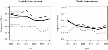
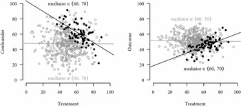
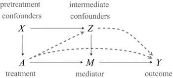
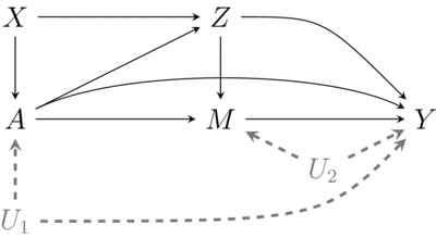
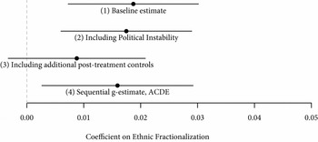
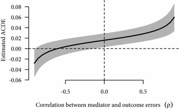
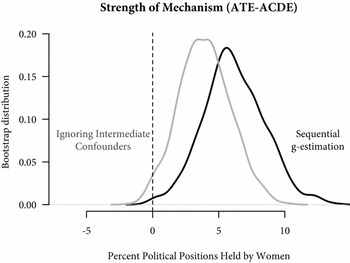
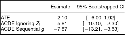
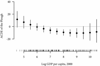




Comments
No Comments have been published for this article.