1. Introduction
The behaviour of free plumes has been well studied since the development of the MTT equations (Morton, Taylor & Turner Reference Morton, Taylor and Turner1956). These describe the dynamics of a turbulent plume in an infinite stratified or unstratified ambient, and require the application of an empirically determined entrainment coefficient to prescribe lateral inflow by turbulent engulfment. By adopting the MTT equations, the behaviour of a free plume in a closed control volume was studied by Baines & Turner (Reference Baines and Turner1969). The associated ‘filling box’ model has fluid from the (descending) plume spreading laterally upon reaching the bottom of the control volume, then forming an ever deepening layer. The top surface of this layer is referred to as the ‘first front’; it approaches the plume source asymptotically for large time,
 $t$
, so that
 $h_{f}\propto t^{2/3}$
, where
 $h_{f}$
is the first front elevation. The inner solution of the filling box flow describes the vertical variation of the plume volume, momentum and buoyancy fluxes. Conversely the outer solution predicts, among other quantities, the first front advection speed. In Baines & Turner’s treatment, the horizontal motion of the discharged plume fluid was omitted; however, this flow was included in the form of a gravity current by later researchers, e.g. Britter (Reference Britter1979), Manins (Reference Manins1979) and Kaye & Hunt (Reference Kaye and Hunt2007).
Whereas a voluminous literature has accumulated on the above convection problem and its application to mixing in chemical storage tanks (Germeles Reference Germeles1975), the built environment (Caulfield & Woods Reference Caulfield and Woods2002; Nabi & Flynn Reference Nabi and Flynn2013) and ocean basins (Manins Reference Manins1979; Hughes & Griffiths Reference Hughes and Griffiths2006), comparatively less work has been conducted to understand plumes and filling box flows in porous media. However, this latter problem is very much deserving of attention because, here again, numerous industrial and environmental applications arise. (i) For instance, consider geological sequestration of supercritical CO
 $_{2}$
(sc-CO
 $_{2}$
) into deep saline aquifers for the purposes of isolating anthropogenic CO
 $_{2}$
(Baines & Worden Reference Baines and Worden2004; Bickle et al.
Reference Bickle, Chadwick, Huppert, Hallworth and Lyle2007). When brine becomes saturated with dissolved sc-CO
 $_{2}$
in the upper layer of aquifers, its density becomes larger than that of the unsaturated brine. There follows the appearance of negatively buoyant plumes that result in convective dissolution of this dense sc-CO
 $_{2}$
–brine mixture into the unsaturated brine below (Ennis-King & Paterson Reference Ennis-King and Paterson2003). Thus in evaluating the long-term efficacy of carbon sequestration, convective dissolution of the injected sc-CO
 $_{2}$
into brine must be considered and this, in turn, requires an understanding of porous media plumes and their mixing with ambient fluid (Neufeld et al.
Reference Neufeld, Hesse, Riaz, Hallworth, Tchelepi and Huppert2010; MacMinn et al.
Reference MacMinn, Neufeld, Hesse and Huppert2012). Moreover, because of the finite horizontal and vertical extents of aquifers, such plumes must often be studied in the context of filling box type flows. (ii) The second application to consider is the dissolution of non-aqueous-phase liquids (NAPL) in the subsurface environment (Khachikian & Harmon Reference Khachikian and Harmon2000; Kueper et al.
Reference Kueper, Wealthall, Smith, Leharne and Lerner2003). NAPL seepage through the vadose zone and into zones containing ground water is primarily driven by density differences between the NAPL and ground water. Because the zones in question may have restricted boundaries, filling box models should again be deployed in quantifying rates of mixing and contamination. Seeking to address some of the flow behaviours specific to these applications, the recent study of Roes, Bolster & Flynn (Reference Roes, Bolster and Flynn2014) considered a filling box flow in a ‘leaky’ porous medium, i.e. one having one or more discrete fissures, which allow for an outflow of discharged plume fluid. Steady state is achieved once this outflow equals the plume volume flux at the level of the (flat, stationary) first front. Note, however, that Roes et al. (Reference Roes, Bolster and Flynn2014) did not examine the transient approach towards steady state nor the case of a reservoir sealed by caprock boundaries devoid of fissures, for which no steady-state solutions exist. Further aspects of Roes et al.’s study are considered below.
Flows in porous media can be divided into the two following categories depending on the value of the Reynolds number,
 $\mathit{Re}=d_{0}U/{\it\nu}$
, where
 $d_{0}$
is the mean grain diameter,
 $U$
is a characteristic velocity that depends upon transport velocity, which we will define in § 2.1, and
 ${\it\nu}$
is the kinematic viscosity: (i) Darcy flow where
 $\mathit{Re}\lesssim O(10)$
, and (ii) non-Darcy flow where
 $\mathit{Re}>O(10)$
(Bear Reference Bear1972; Dullien Reference Dullien1992). A second, equally important, non-dimensional number in (variable-component, miscible) porous media flow is the Péclet number,
 $\mathit{Pe}=d_{0}U{\it\tau}/D_{d}$
, in which
 $D_{d}$
is the molecular diffusion coefficient and
 ${\it\tau}~({>}1)$
is the tortuosity constant, which is defined as the ratio of the actual path length travelled by a solute molecule to the distance it would travel in the absence of a porous medium. The Péclet number characterizes the importance of advection versus diffusion, with diffusive transport playing a subordinate role to mechanical dispersive transport when
 $\mathit{Pe}\gg O(1)$
. The combined influence of diffusion and dispersion can be modelled by defining the following transport coefficient:
 $$\begin{eqnarray}D=d_{0}U\left(1+\frac{1}{\mathit{Pe}}\right)\end{eqnarray}$$
(Houseworth Reference Houseworth1984; Delgado Reference Delgado2007). When
 $\mathit{Pe}\ll O(1)$
,
 $D\simeq D_{d}/{\it\tau}$
; however, when
 $\mathit{Pe}\gg O(1)$
,
 $D\simeq d_{0}U$
. In this latter limit, it is appropriate to refer to
 $D$
as the dispersion coefficient.
The dynamics of rectilinear line plumes in porous media was first studied by Wooding (Reference Wooding1963) for Darcy flow with
 $\mathit{Pe}\ll O(1)$
. Starting from mass continuity, Darcy’s law and a solute transport equation, Wooding (Reference Wooding1963) derived a similarity solution based on the assumption that the plume is long and thin. On this basis, he obtained the following equation for the variation of the plume volume flux,
 $Q$
, with the vertical coordinate,
 $x$
:
 $$\begin{eqnarray}Q=\left(\frac{36D{\it\phi}F_{0}k{\it\Lambda}^{2}x}{{\it\nu}}\right)^{1/3}.\end{eqnarray}$$
Here
 ${\it\phi}$
is the porosity,
 $F_{0}$
is the source buoyancy flux,
 $k$
is the permeability and
 ${\it\Lambda}$
is the source width in the third dimension.
Roes et al. (Reference Roes, Bolster and Flynn2014) adopted Wooding’s equations into the
 $\mathit{Pe}\gg O(1)$
filling box framework, but could only do so by making a limiting assumption on
 $D$
, namely that its numerical value was the same everywhere inside the porous medium. Although there exists some practical justification for this approach, this assumption is, strictly speaking, incorrect:
 $D$
depends upon the flow speed, and the flow speed, in turn, varies both horizontally and vertically. In fact, Lai (Reference Lai1991) considered the case of spatially variable
 $D$
. However, Lai’s analysis was complicated by the fact that, as with the earlier investigation by Chen & Ho (Reference Chen and Ho1986), he assumed a non-Darcy flow regime. Thus the Darcy equations were replaced by the Darcy–Forchheimer equations, which are obtained by introducing Dupuit–Forchheimer inertial terms into the Darcy equations (Nield & Kuznetsov Reference Nield and Kuznetsov2013). These inertial terms are proportional to the square of the transport velocity and also include a drag coefficient whose value depends on the geometry of the porous media. In these studies of non-Darcy plumes, it was proved that no similarity solution exists, and hence solutions were instead presented in terms of a non-similar variable, whose magnitude depended on various physical parameters, e.g. the permeability and fluid viscosity.
Here we synthesize these previous approaches by assuming Darcy flow with a spatially variable
 $D$
. Our objectives are twofold: (i) to derive self-similar plume equations in a rectilinear geometry germane to this case, and (ii) to use the associated solutions to examine the time-dependent behaviour of porous media filling box flows, from which various pertinent flow time scales can be estimated. Importantly, our analysis includes a description of the gravity current dynamics associated with plume outflow along the impermeable bottom boundary. As noted above, these dynamics are sometimes omitted when studying turbulent free plumes. The theory is validated (where possible) by comparison with analogue laboratory experiments that employ salt water and fresh water, respectively, as the source and ambient fluids.
The rest of the paper is organized as follows. Our plume solution is given in § 2.1 whereas §§ 2.2 and 2.3 describe, respectively, the gravity current and the ascending first front. Thereafter, in § 3, the laboratory experiments are discussed. This description is followed by a comparison between theory and experiment, which appears in § 4. Finally, § 5 presents conclusions of this work and identifies topics for future study.
2. Theory
2.1. Plume in an unbounded medium
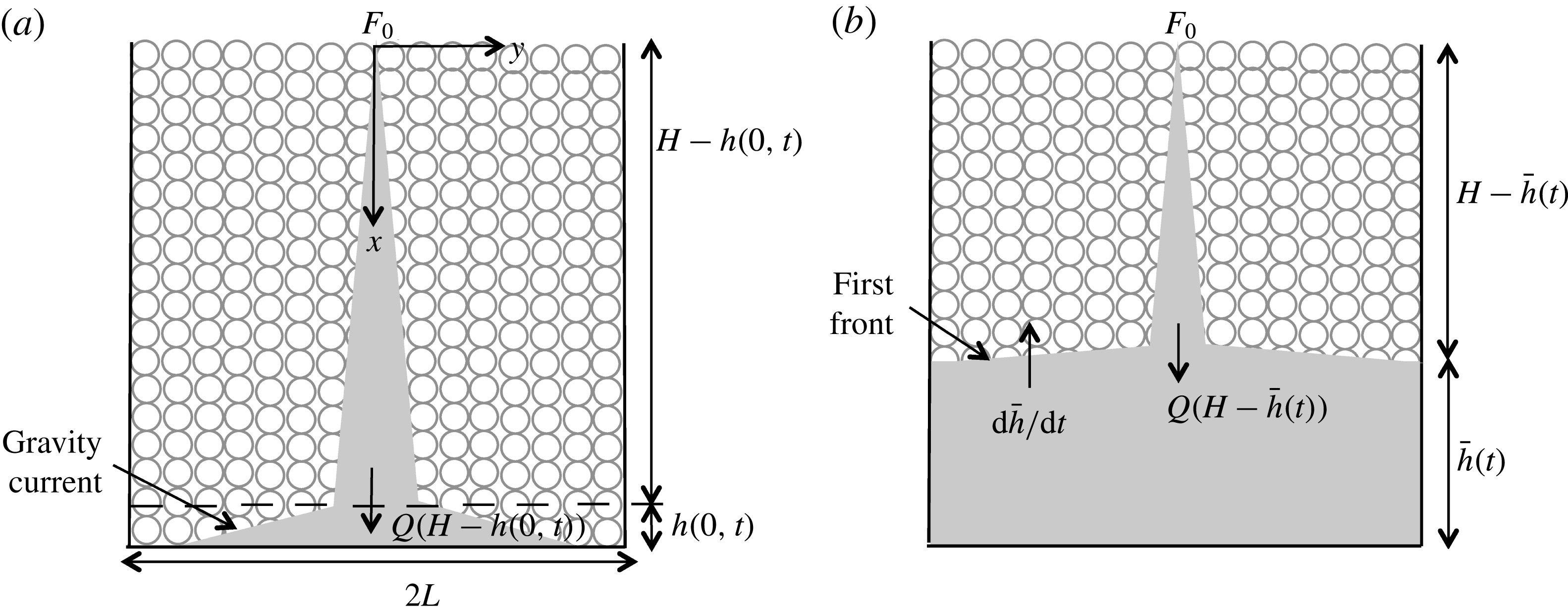
To derive a solution for laminar plume flow in a porous medium, we begin by presenting the governing equations based on mass and momentum continuity, solute transport and a linear equation of state. In contrast to Wooding (Reference Wooding1963) and Roes et al. (Reference Roes, Bolster and Flynn2014), we consider a dispersion coefficient that varies in
 $x$
and
 $y$
, where the
 $x$
and
 $y$
directions are defined in figure 1.
Convection in a confined porous medium: (a) plume and gravity current flow; (b) advection of the first front towards the source.

The flow is assumed to be steady, Boussinesq and two-dimensional rectilinear, and the ambient is assumed to remain unstratified above the first front so that the governing equations read
 $$\begin{eqnarray}\displaystyle & \displaystyle \frac{\partial u}{\partial x}+\frac{\partial v}{\partial y}=0 & \displaystyle \;[\text{mass continuity}],\end{eqnarray}$$
 $$\begin{eqnarray}\displaystyle & \displaystyle \frac{1}{{\it\rho}_{0}}\frac{\partial P}{\partial x}+\frac{{\it\nu}}{k}u=\frac{g{\it\rho}}{{\it\rho}_{0}} & \displaystyle \;[\text{momentum cont. in }x],\end{eqnarray}$$
 $$\begin{eqnarray}\displaystyle & \displaystyle \frac{1}{{\it\rho}_{0}}\frac{\partial P}{\partial y}+\frac{{\it\nu}}{k}v=0 & \displaystyle \;[\text{momentum cont. in }y],\end{eqnarray}$$
 $$\begin{eqnarray}\displaystyle & \displaystyle \frac{1}{{\it\phi}}\left(u\frac{\partial C}{\partial x}+v\frac{\partial C}{\partial y}\right)=\frac{\partial }{\partial x}\left(D_{L}\frac{\partial C}{\partial x}\right)+\frac{\partial }{\partial y}\left(D_{T}\frac{\partial C}{\partial y}\right) & \displaystyle \;[\text{solute transport}],\end{eqnarray}$$
 $$\begin{eqnarray}\displaystyle & \displaystyle {\it\rho}={\it\rho}_{0}(1+{\it\beta}C) & \displaystyle \;[\text{linear equation of state}].\nonumber\\ \displaystyle & & \displaystyle\end{eqnarray}$$
 $P$
is the fluid pressure,
 $C$
is the solute concentration and
 ${\it\beta}$
is the solute contraction coefficient. Moreover,
 ${\it\rho}$
is the fluid density, whose far-field value is
 ${\it\rho}_{0}$
, corresponding to a solute concentration of zero. Furthermore,
 $D_{L}$
and
 $D_{T}$
are the longitudinal and transverse dispersion coefficients.
The momentum equations, (2.2) and (2.3), are combined to eliminate the fluid pressure, whereby
 $$\begin{eqnarray}\frac{{\it\nu}}{k}\left(\frac{\partial u}{\partial y}-\frac{\partial v}{\partial x}\right)=\frac{g}{{\it\rho}_{0}}\frac{\partial {\it\rho}}{\partial y}.\end{eqnarray}$$
We then apply Wooding’s boundary layer approximation so that
 $$\begin{eqnarray}\left|\frac{\partial v}{\partial x}\right|\ll \left|\frac{\partial u}{\partial y}\right|\quad \text{and}\quad \left|\frac{\partial }{\partial x}\left(D_{L}\frac{\partial C}{\partial x}\right)\right|\ll \left|\frac{\partial }{\partial y}\left(D_{T}\frac{\partial C}{\partial y}\right)\right|.\end{eqnarray}$$
The validity of the latter boundary layer approximation is outlined at the end of § 2.1.
Following Houseworth (Reference Houseworth1984), Delgado (Reference Delgado2007) and others, for
 $\mathit{Pe}\gg O(1)$
, the transverse dispersion coefficient can be expressed as
 $$\begin{eqnarray}D_{T}\simeq {\it\alpha}u.\end{eqnarray}$$
Here
 ${\it\alpha}$
is the transverse dispersivity, and its value shall, consistent with the turbulent plume entrainment coefficient (Morton et al.
Reference Morton, Taylor and Turner1956), be determined based on experimental measurement. The above representation for
 $D_{T}$
, in particular the use of
 $u$
rather than the horizontal transport velocity
 $v$
, and the incorporation of
 ${\it\alpha}$
follows from the methodology of Lai (Reference Lai1991). Finally, and for
 $\mathit{Pe}\gg O(1)$
, we can now make a connection between
 $u$
and the characteristic velocity,
 $U$
, that appears in (1.1), i.e.
 $U={\it\alpha}u/d_{0}$
.
On the basis of the above discussion, (2.4) becomes
 $$\begin{eqnarray}u\frac{\partial C}{\partial x}+v\frac{\partial C}{\partial y}={\it\alpha}{\it\phi}\frac{\partial }{\partial y}\left(u\frac{\partial C}{\partial y}\right).\end{eqnarray}$$
Furthermore, a streamfunction,
 ${\it\psi}$
, is introduced such that
 $u=\partial {\it\psi}/\partial y$
and
 $v=-\partial {\it\psi}/\partial x$
. Equations (2.6) and (2.9) can then be rewritten as
 $$\begin{eqnarray}\displaystyle & \displaystyle \frac{\partial ^{2}{\it\psi}}{\partial y^{2}}=\frac{g{\it\beta}k}{{\it\nu}}\frac{\partial C}{\partial y}, & \displaystyle\end{eqnarray}$$
 $$\begin{eqnarray}\displaystyle & \displaystyle \frac{\partial {\it\psi}}{\partial y}\frac{\partial C}{\partial x}-\frac{\partial {\it\psi}}{\partial x}\frac{\partial C}{\partial y}={\it\alpha}{\it\phi}\left(\frac{\partial ^{2}{\it\psi}}{\partial y^{2}}\frac{\partial C}{\partial y}+\frac{\partial {\it\psi}}{\partial y}\frac{\partial ^{2}C}{\partial y^{2}}\right), & \displaystyle\end{eqnarray}$$
 $$\begin{eqnarray}{\it\psi}=A_{1}x^{p}\mathscr{F}({\it\eta}),\quad C=A_{2}x^{q}\mathscr{G}({\it\eta}),\end{eqnarray}$$
where the self-similar variable,
 ${\it\eta}$
, is defined as
 ${\it\eta}=A_{3}y/x^{n}$
. The constants
 $p$
,
 $q$
,
 $n$
,
 $A_{1}$
,
 $A_{2}$
and
 $A_{3}$
will be determined shortly. Applying (2.12) in (2.10) yields
 $$\begin{eqnarray}A_{1}x^{p}\mathscr{F}^{\prime \prime }\left(\frac{A_{3}}{x^{n}}\right)^{2}=\frac{g{\it\beta}k}{{\it\nu}}A_{2}x^{q}\mathscr{G}^{\prime }\frac{A_{3}}{x^{n}}.\end{eqnarray}$$
Thus,
 $\mathscr{G}({\it\eta})=\mathscr{F}^{\prime }({\it\eta})\equiv \text{d}\mathscr{F}/\text{d}{\it\eta}$
,
 $n=p-q$
and
 $A_{2}=A_{1}A_{3}{\it\nu}/(g{\it\beta}k)$
. Hence, (2.11) becomes
 $$\begin{eqnarray}\displaystyle & & \displaystyle x^{2q-1}\{[q\mathscr{F}^{\prime }-(p-q)\mathscr{F}^{\prime \prime }{\it\eta}]\mathscr{F}^{\prime }-[\,p\mathscr{F}-(p-q)\mathscr{F}^{\prime }{\it\eta}]\mathscr{F}^{\prime \prime }\}\nonumber\\ \displaystyle & & \displaystyle \quad ={\it\alpha}{\it\phi}A_{3}^{2}x^{2(2q-p)}(\mathscr{F}^{\prime \prime }\mathscr{F}^{\prime \prime }+\mathscr{F}^{\prime \prime \prime }\mathscr{F}^{\prime }).\end{eqnarray}$$
The factors of
 $x$
that appear on the left- and right-hand sides of the equation disappear provided
 $p-q=1/2$
. Equation (2.14) is further simplified by selecting
 $A_{3}=1/\sqrt{{\it\alpha}{\it\phi}}$
whereupon
 $$\begin{eqnarray}\mathscr{F}^{\prime \prime \prime }\mathscr{F}^{\prime }+\mathscr{F}^{\prime \prime }\mathscr{F}^{\prime \prime }+p\mathscr{F}^{\prime \prime }\mathscr{F}-q\mathscr{F}^{\prime }\mathscr{F}^{\prime }=0.\end{eqnarray}$$
To determine the values for
 $p$
and
 $q$
, we recall that the buoyancy flux,
 $F_{0}$
, is conserved, i.e. it is independent of the vertical coordinate in an unstratified medium. Formally,
 $F_{0}$
is defined as
 $$\begin{eqnarray}F_{0}={\it\Lambda}\int _{-\infty }^{\infty }ug^{\prime }\,\text{d}y,\end{eqnarray}$$
where
 $g^{\prime }=g({\it\rho}-{\it\rho}_{0})/{\it\rho}_{0}\equiv g{\it\beta}C$
is the reduced gravity. By applying the above results, it can be shown that
 $$\begin{eqnarray}F_{0}={\it\Lambda}g{\it\beta}A_{1}A_{2}x^{(p+q)}\int _{-\infty }^{\infty }{\mathscr{F}^{\prime }}^{2}\,\text{d}{\it\eta},\end{eqnarray}$$
which implies that
 $p+q=0$
. But we previously showed that
 $p-q=1/2$
and therefore
 $p=1/4$
and
 $q=-1/4$
. Consequently, (2.15) takes the form
 $$\begin{eqnarray}\mathscr{F}^{\prime \prime \prime }\mathscr{F}^{\prime }+\mathscr{F}^{\prime \prime }\mathscr{F}^{\prime \prime }+{\textstyle \frac{1}{4}}\mathscr{F}^{\prime \prime }\mathscr{F}+{\textstyle \frac{1}{4}}\mathscr{F}^{\prime }\mathscr{F}^{\prime }=(\mathscr{F}^{\prime \prime }\mathscr{F}^{\prime })^{\prime }+{\textstyle \frac{1}{4}}(\mathscr{F}^{\prime }\mathscr{F})^{\prime }=0.\end{eqnarray}$$
In solving (2.18), we recall the assumption that
 $D\simeq d_{0}\bar{U}$
, i.e.
 $\mathit{Pe}\gg O(1)$
. In the neighbourhood of the plume centreline, this is a reasonable approximation; however, its validity is highly suspect far away from the centreline where flow velocities become small. We therefore restrict ourselves to finding an ‘inner’ solution to (2.15), valid in the limit of small
 $y$
(small
 ${\it\eta}$
). In the outer region, by contrast, spatial variations in
 $u$
,
 $v$
or
 $S$
are ignored. Such a division of the flow into inner and outer regions would be inappropriate in the case of constant
 $D$
(Wooding Reference Wooding1963; Roes et al.
Reference Roes, Bolster and Flynn2014), but is, in fact, not at all dissimilar to the approach followed in the ‘top hat’ description of free turbulent plumes, where molecular diffusive effects are likewise ignored (Morton et al.
Reference Morton, Taylor and Turner1956; Linden, Lane-Serff & Smeed Reference Linden, Lane-Serff and Smeed1990). We therefore proceed by integrating (2.18) remembering that
 $\mathscr{F}^{\prime }({\it\eta})=\mathscr{G}({\it\eta})$
prescribes the non-dimensional solute concentration. This concentration cannot be negative and must vanish altogether in the far field; symbolically,
 $C(x,y)>0~\Rightarrow ~\mathscr{F}^{\prime }({\it\eta})>0$
and
 $C(x,\pm \infty )=C_{0}~\Rightarrow ~\mathscr{F}^{\prime }(\pm \infty )=0$
. Symmetry suggests, moreover, that the concentration must be identical left and right, so that
 $C(x,y)=C(x,-y)~\Rightarrow ~\mathscr{F}^{\prime }({\it\eta})=\mathscr{F}^{\prime }(-{\it\eta})$
. Symmetry also requires that
 ${\it\psi}(x,0)=0$
so that
 $\mathscr{F}(0)=0$
. Therefore, it can be shown that
 $$\begin{eqnarray}\mathscr{F}=\left\{\begin{array}{@{}ll@{}}-\displaystyle c, & {\it\eta}<-{\rm\pi},\\ \displaystyle c\sin \frac{{\it\eta}}{2}, & -{\rm\pi}<{\it\eta}<{\rm\pi},\\ \displaystyle c, & {\it\eta}>{\rm\pi},\end{array}\right.\!\!\!\!\quad \text{and}\quad \mathscr{G}=\mathscr{F}^{\prime }=\left\{\begin{array}{@{}ll@{}}\displaystyle \frac{c}{2}\cos \frac{{\it\eta}}{2}, & -{\rm\pi}<{\it\eta}<{\rm\pi},\\ 0, & |{\it\eta}|>{\rm\pi}.\end{array}\right.\end{eqnarray}$$
Here
 $c$
is a constant of integration and will automatically disappear shortly. Note that (2.19) is the only symmetric non-trivial solution to (2.18) satisfying
 $\mathscr{G}=\mathscr{F}^{\prime }\geqslant 0$
. Now on applying (2.17), and recalling that
 $A_{2}=A_{1}A_{3}{\it\nu}/(g{\it\beta}k)$
, we find
 $$\begin{eqnarray}A_{1}=\left(\frac{F_{0}k}{{\it\Lambda}{\it\nu}}\frac{\sqrt{{\it\alpha}{\it\phi}}}{\displaystyle \int _{-\infty }^{\infty }{\mathscr{F}^{\prime }}^{2}\,\text{d}{\it\eta}}\right)^{1/2}.\end{eqnarray}$$
Equation (2.19) can then be combined with (2.12) to determine the volume flux,
 $Q$
, of the plume. More specifically,
 $$\begin{eqnarray}Q={\it\Lambda}\int _{-\infty }^{\infty }u\,\text{d}y=\left[\left(\frac{16F_{0}k{\it\Lambda}}{{\rm\pi}{\it\nu}}\right)^{2}{\it\phi}{\it\alpha}x\right]^{1/4}.\end{eqnarray}$$
Similarly, the plume momentum flux and mean reduced gravity are found to be, respectively,
 $$\begin{eqnarray}M=\frac{F_{0}k}{{\it\nu}}\quad \text{and}\quad \bar{g}^{\prime }=\frac{F_{0}}{Q}=\left[\left(\frac{{\rm\pi}F_{0}{\it\nu}}{16k{\it\Lambda}}\right)^{2}\frac{1}{{\it\phi}{\it\alpha}x}\right]^{1/4}.\end{eqnarray}$$
Note that
 $Q$
and
 $\bar{g}^{\prime }$
are proportional to
 $x^{1/4}$
and
 $x^{-1/4}$
, respectively, whereas in previous investigations, such as Wooding (Reference Wooding1963) and Roes et al. (Reference Roes, Bolster and Flynn2014), where
 $\mathit{Pe}\lesssim O(1)$
, these quantities are proportional to
 $x^{1/3}$
and
 $x^{-1/3}$
. The formula for
 $M$
is unchanged, however, because our plumes plus those of Wooding (Reference Wooding1963) satisfy the conditions for Darcy flow.
Equation (2.21) is derived in the limit of an ideal plume whereby
 $Q\rightarrow 0$
as
 $x\rightarrow 0$
. However, for a non-ideal plume, which has a finite source volume flux, this assumption cannot be applied. Therefore, a virtual origin correction is determined by extrapolating the flow to negative
 $x$
values and a fictitious point,
 $x=-x_{0}$
, where the plume volume flux vanishes (Wooding Reference Wooding1963; see also Hunt & Kaye Reference Hunt and Kaye2001). More formally,
 $x_{0}$
is given by
 $$\begin{eqnarray}x_{0}=\frac{1}{{\it\phi}{\it\alpha}}\left(\frac{{\rm\pi}{\it\nu}}{16F_{0}k{\it\Lambda}}\right)^{2}{Q_{0}}^{4},\end{eqnarray}$$
so that the plume volume flux and mean reduced gravity are given, respectively, by
 $$\begin{eqnarray}Q=\left[\left(\frac{16F_{0}k{\it\Lambda}}{{\rm\pi}{\it\nu}}\right)^{2}{\it\phi}{\it\alpha}(x+x_{0})\right]^{1/4}\end{eqnarray}$$
and
 $$\begin{eqnarray}\bar{g}^{\prime }=g{\it\beta}\bar{C}=\left[\left(\frac{{\rm\pi}F_{0}{\it\nu}}{16k{\it\Lambda}}\right)^{2}\frac{1}{{\it\phi}{\it\alpha}(x+x_{0})}\right]^{1/4}.\end{eqnarray}$$
We prefer to think of solute concentration in terms of its influence on buoyancy, thus our preference for using
 $\bar{g}^{\prime }$
in place of
 $\bar{C}$
. But the relationship between the two is, by virtue of the linear equation of state (2.5), very direct, as confirmed by the above equation.
Finally, we verify the validity of the boundary layer approximation made in (2.7) by estimating, using scaling analysis, the range of
 $D_{L}$
and
 $D_{T}$
for which the stated inequality holds. When (2.7) is valid,
 $$\begin{eqnarray}\frac{D_{L}C}{L_{x}^{2}}\ll \frac{D_{T}C}{L_{y}^{2}}\quad \text{or}\quad \frac{D_{L}}{D_{T}}\ll \left(\frac{L_{x}}{L_{y}}\right)^{2},\end{eqnarray}$$
where
 $L_{x}$
and
 $L_{y}$
, respectively, denote characteristic vertical and horizontal length scales associated with the plume. Given the finite size of the control volume shown schematically in figure 1, we choose
 $L_{x}=H$
. Conversely,
 $L_{y}$
is defined to be the plume width at
 $x=H$
; following from the self-similar solution obtained in (2.19), it can be shown that
 $L_{y}\sim {\rm\pi}\sqrt{{\it\alpha}H}$
. Thus (2.26) holds provided
 $$\begin{eqnarray}\frac{D_{L}}{D_{T}}\ll \frac{H}{{\rm\pi}^{2}{\it\alpha}}.\end{eqnarray}$$
Using results from § 4, it can be argued that
 $1/({\rm\pi}^{2}{\it\alpha})\sim O(0.1)~\text{cm}^{-1}$
, at least for the experiments of interest here. Moreover,
 $H\sim O(10)~\text{cm}$
and therefore, in the present context,
 $H/({\rm\pi}^{2}{\it\alpha})\sim O(10^{2})$
. By contrast, we expect
 $D_{L}/D_{T}$
to be significantly less: according to Bear & Verruijt (Reference Bear and Verruijt1987),
 $D_{L}/D_{T}\simeq 100$
only for large Péclet numbers, i.e.
 $\mathit{Pe}\sim O(10^{6})$
, roughly three orders of magnitude greater than the values of
 $\mathit{Pe}$
relevant to our laboratory experiments. We therefore expect (2.27) to be satisfied both experimentally and, equally importantly, in real geophysical flows for which
 $H$
and
 ${\it\alpha}$
are expected to be larger and smaller, respectively, than the values germane to § 3.
It should also be recalled that numerous authors (Guin, Kessler & Greenkorn Reference Guin, Kessler and Greenkorn1972) recommend application of a dispersion tensor in (2.4) according to which there must appear the additional right-hand side terms
 $\partial (D_{xy}(\partial C/\partial y))/\partial x$
and
 $\partial (D_{yx}(\partial C/\partial x))/\partial y$
in which
 $D_{xy}=D_{yx}$
is the off-diagonal component of the (symmetric)
 $2\times 2$
dispersion tensor. Using a similar analysis to that described in the previous paragraph, it can likewise be shown that the contribution of these additional terms is small compared to
 $\partial (D_{T}(\partial C/\partial y))/\partial y$
.
2.2. Gravity current
When the plume fluid collides with the (impermeable) bottom boundary of the control volume, a pair of gravity currents, travelling in the
 $+y$
and
 $-y$
directions, are formed (Manins Reference Manins1979; Kaye & Hunt Reference Kaye and Hunt2007). Although the flow initiates at the instant that the source nozzle is ‘switched on’, we take
 $t=0$
to be the time when plume fluid first reaches the bottom boundary. We justify this assumption as follows. Using (2.12) and (2.19), it is straightforward to estimate the time,
 $t_{R}$
, that a fluid particle resides within the plume whilst flowing a vertical distance
 $H$
. (The residence time associated with flow within a thermal is expected to be larger than, but still comparable to, the residence time associated with flow within a plume.) Comparing
 $t_{R}$
against the time,
 $t_{L}$
, required for the gravity current to reach the lateral sidewalls, we find that
 $t_{R}/t_{L}\sim O(10^{-1})$
for the geometry of interest here. (The time scale
 $t_{L}$
is defined more precisely below.) In like fashion,
 $t_{R}/t_{H}\sim O(10^{-2})$
, where
 $t_{H}$
, defined in § 2.3, is the time required for the first front to reach the top of the control volume. By ignoring the flow dynamics within the time interval
 $t_{R}$
, we implicitly exclude from considering control volumes that are tall and narrow. However, this case is not representative of many real geophysical scenarios where
 $L\gg H$
and, in any event, is unlikely to yield well-defined gravity currents of the type investigated below in § 2.2.
The propagation of a gravity current through a porous medium has been described by Huppert & Woods (Reference Huppert and Woods1995) – only a brief review of their formulation is provided below.
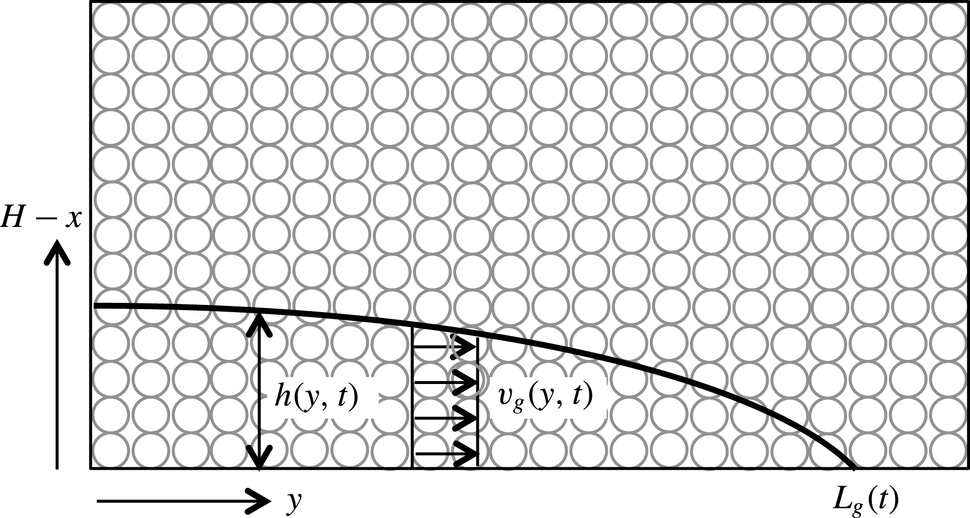
Gravity current flow in a porous medium.

Presuming a hydrostatic flow, the gravity current horizontal flow speed,
 $v_{g}$
, is depth-independent and varies with
 $\partial h/\partial y$
, where
 $h$
is the interface height (see figure 2) according to
 $$\begin{eqnarray}v_{g}=-\frac{kg_{g}^{\prime }}{{\it\nu}}\frac{\partial h}{\partial y}\end{eqnarray}$$
(Huppert & Woods Reference Huppert and Woods1995, equation (2.5)). Here
 $g_{g}^{\prime }$
is the reduced gravity of the discharged plume fluid turned gravity current fluid. Strictly speaking,
 $g_{g}^{\prime }$
is a function of
 $t$
; however, we verify below that the time rate of change of
 $g_{g}^{\prime }$
is small enough to be considered negligible, at least for the problem of interest here.
The equation of local volume flux balance reads
 $$\begin{eqnarray}{\it\phi}\frac{\partial h}{\partial t}=-\frac{\partial }{\partial y}\left[\int _{0}^{h(y,t)}v_{g}(y,t)\,\text{d}(H-x)\right].\end{eqnarray}$$
On substituting (2.28) into (2.29), it can easily be shown that
 $$\begin{eqnarray}\frac{\partial h}{\partial t}-S\frac{\partial }{\partial y}\left(h\frac{\partial h}{\partial y}\right)=0,\end{eqnarray}$$
where
 $S=kg_{g}^{\prime }/{\it\nu}{\it\phi}$
. Also, the boundary condition at the leading edge of the gravity current and the mass conservation equation are given by
 $$\begin{eqnarray}h(L_{g}(t),t)=0\quad \text{and}\quad {\it\phi}\displaystyle \int _{0}^{L_{g}(t)}h(y,t)\,\text{d}y=V(t),\end{eqnarray}$$
respectively (Huppert & Woods Reference Huppert and Woods1995, equation (3.5)). Here
 $V$
is the total volume of discharged plume fluid turned gravity current fluid measured from the initial instant, when the plume first reaches the bottom surface, up to time
 $t$
, at which point the gravity current is
 $L_{g}$
units long.
The methodology presented by Huppert & Woods (Reference Huppert and Woods1995) is adopted to solve (2.30); thus, we seek a self-similar solution of the form
 $$\begin{eqnarray}h=\left(\frac{Q_{g}^{2}}{S}t\right)^{1/3}\!\mathscr{H}({\it\xi})\quad \text{where }{\it\xi}=\left(\frac{1}{Q_{g}S}\right)^{1/3}\!\frac{y}{t^{2/3}}\text{ and }t{\nrightarrow}0.\end{eqnarray}$$
Here
 $Q_{g}$
is the volume flux per unit span of the discharged plume fluid turned gravity current fluid. With a similar argument as above for
 $g_{g}^{\prime }$
, we neglect the time dependence of
 $Q_{g}$
, for which a verification is presented at the end of this section. After some simplification, the partial differential equation (2.30) can be rewritten as the following ordinary differential equation (ODE) in
 ${\it\xi}$
:
 $$\begin{eqnarray}3\mathscr{H}^{\prime \prime }\mathscr{H}^{\prime }+3\mathscr{H}^{\prime }\mathscr{H}^{\prime }+2{\it\xi}\mathscr{H}^{\prime }-\mathscr{H}=0.\end{eqnarray}$$
The associated boundary conditions, which come from (2.31), read
 $$\begin{eqnarray}\mathscr{H}({\it\lambda})=0\quad \text{and}\quad {\it\phi}\int _{0}^{{\it\lambda}}\mathscr{H}\,\text{d}{\it\xi}=1,\end{eqnarray}$$
where
 ${\it\lambda}$
is the dimensionless length of the gravity current, so that
 $\text{max}({\it\xi})={\it\lambda}$
. A numerical solution is obtained for (2.33) by employing a shooting method to find
 $\mathscr{H}({\it\xi}=0)$
and
 ${\it\lambda}$
. Note that, in this equation,
 ${\it\xi}$
is the independent variable of integration, not
 $t$
. Therefore, we initialize our solver using a ‘clever guess’ for the appropriate condition at
 ${\it\xi}=0$
and solve the ODE. We then look to see whether the volume conservation equation
 ${\it\phi}\int _{0}^{{\it\lambda}}\mathscr{H}\,\text{d}{\it\xi}=1$
is satisfied given that
 $\mathscr{H}({\it\lambda})=0$
. The ‘clever guess’ is then updated and the process repeated till the solution converges. Numerical values of
 $\mathscr{H}({\it\xi}=0)$
and
 ${\it\lambda}$
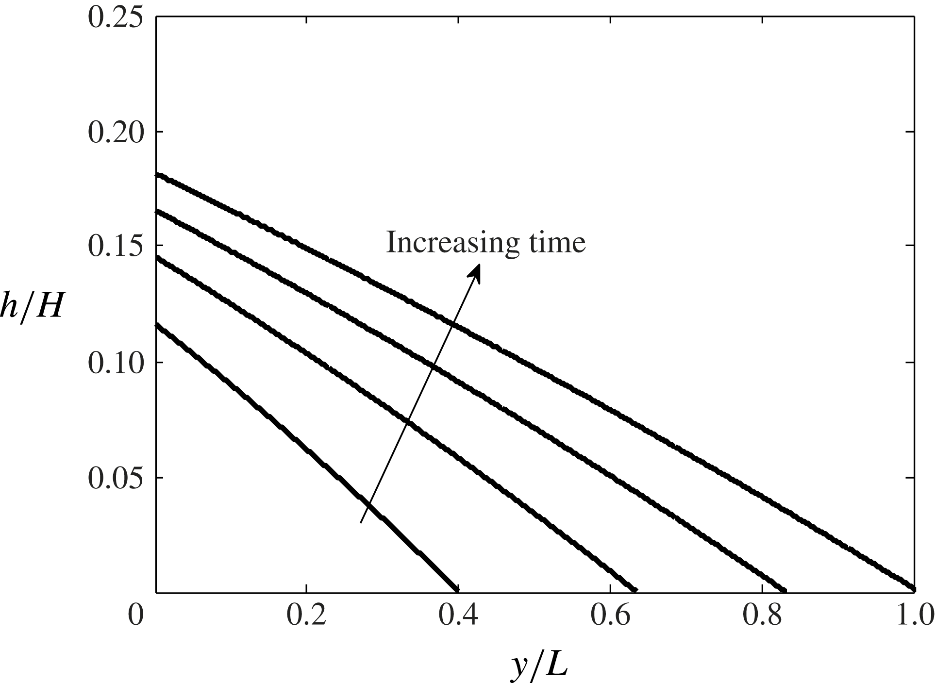
are found to be, respectively, 2.470 and 2.046. The solution obtained is then used to predict the gravity current shape as a function of time, for which sample results are exhibited in figure 3. Because
 $t=0$
is outside of the region of interest here, the final solution is plotted only for
 $t\gg 0$
.
Gravity current height and length versus time. The non-dimensional time increment is
 $0.25t_{L}$
, starting with
 $t=0.25t_{L}$
for the lowest curve and finishing with
 $t=t_{L}$
with the gravity current front located at
 $y/L=1$
. Also,
 $S=kg^{\prime }/{\it\phi}{\it\nu}=0.6~\text{cm}~\text{s}^{-1}$
, where
 ${\it\phi}=0.38$
.

It should be noted that the result obtained from the similarity solution is valid only when the gravity current is long and thin, i.e.
 $h(0,t)\ll L_{g}(t)$
. Here
 $L_{g}(t)$
is the length of the gravity current and is given as
 $$\begin{eqnarray}L_{g}={\it\lambda}(Q_{g}S)^{1/3}t^{2/3}.\end{eqnarray}$$
Furthermore, the time required by the gravity current front to reach the sidewall of the control volume, which is at a horizontal distance
 $L$
from the source, is
 $$\begin{eqnarray}t_{L}=\left[\left(\frac{L}{{\it\lambda}}\right)^{3}\frac{1}{Q_{g}S}\right]^{1/2}.\end{eqnarray}$$
From (2.35) and (2.36), a straightforward relation between the dimensionless length and time can be derived as
 $$\begin{eqnarray}\frac{L_{g}}{L}=\left(\frac{t}{t_{L}}\right)^{2/3}.\end{eqnarray}$$
Note also that, when
 $t=t_{L}$
, the mean height of the gravity current is given by
 $$\begin{eqnarray}\bar{h}_{t_{L}}=\frac{1}{L}\int _{0}^{L}h(y,t_{L})\,\text{d}y=\frac{1}{{\it\lambda}}\left(\frac{Q_{g}^{2}}{{\it\phi}^{3}S}t_{L}\right)^{1/3}.\end{eqnarray}$$
This mean height of the gravity current will be used in § 4 when comparing the theoretical model with the experimental measurements.
From (2.24) and (2.25) we observe that
 $Q_{g}\propto (1-h/H)^{1/4}$
and
 $g_{g}^{\prime }\propto (1-h/H)^{-1/4}$
, respectively. Furthermore,
 $h/H\ll 1$
(see figure 3). These observations support our assumption that the time rates of change of
 $Q_{g}$
and
 $g_{g}^{\prime }$
are negligible. For instance, the change in
 $Q_{g}$
and
 $g_{g}^{\prime }$
between the times
 $t=0.25t_{L}$
and
 $t=t_{L}$
for the curves presented in figure 3 are
 $-1.59\,\%$
and 1.59 %, respectively, whereas the increase in time is 300 %.
2.3. First front
After the gravity current reaches the sidewall of the control volume, the dense fluid near the sidewall begins to move primarily vertically. Following the terminology introduced by Baines & Turner (Reference Baines and Turner1969), we refer to the interface between the discharged plume fluid and the overlying ambient fluid as the first front. Whereas the first front evolves in time and becomes horizontal in the long-time limit, its initial profile is prescribed by the shape of the gravity current at
 $t=t_{L}$
. For
 $t>t_{L}$
, the pressure remains hydrostatic and therefore the horizontal velocity below the first front remains independent of
 $x$
. Hence, (2.30) can be employed to describe the spatio-temporal evolution of the first front. In this case, however, one must replace the front condition (2.31a
) with a no-flux condition at the (impermeable) sidewalls. Symbolically
 $$\begin{eqnarray}\partial h/\partial y=0\quad \text{when }y=\pm L\text{ and }t>t_{L}.\end{eqnarray}$$
The second boundary condition is obtained from a straightforward extension of (2.31b ), i.e.
 $$\begin{eqnarray}{\it\phi}\int _{0}^{L}[h(y,t-t_{L})-h(y,t_{L})]\,\text{d}y=V(t-t_{L}).\end{eqnarray}$$
The finite length of the box obviously imposes an external length scale on the problem at hand and, as a consequence, no self-similar solution is possible. However, a numerical solution can be obtained by applying a semi-implicit finite difference scheme (Causon & Mingham Reference Causon and Mingham2010). We rewrite (2.30) in the form
 $$\begin{eqnarray}\frac{\partial h}{\partial t}=\frac{S}{2}\frac{\partial ^{2}h^{2}}{\partial y^{2}}.\end{eqnarray}$$
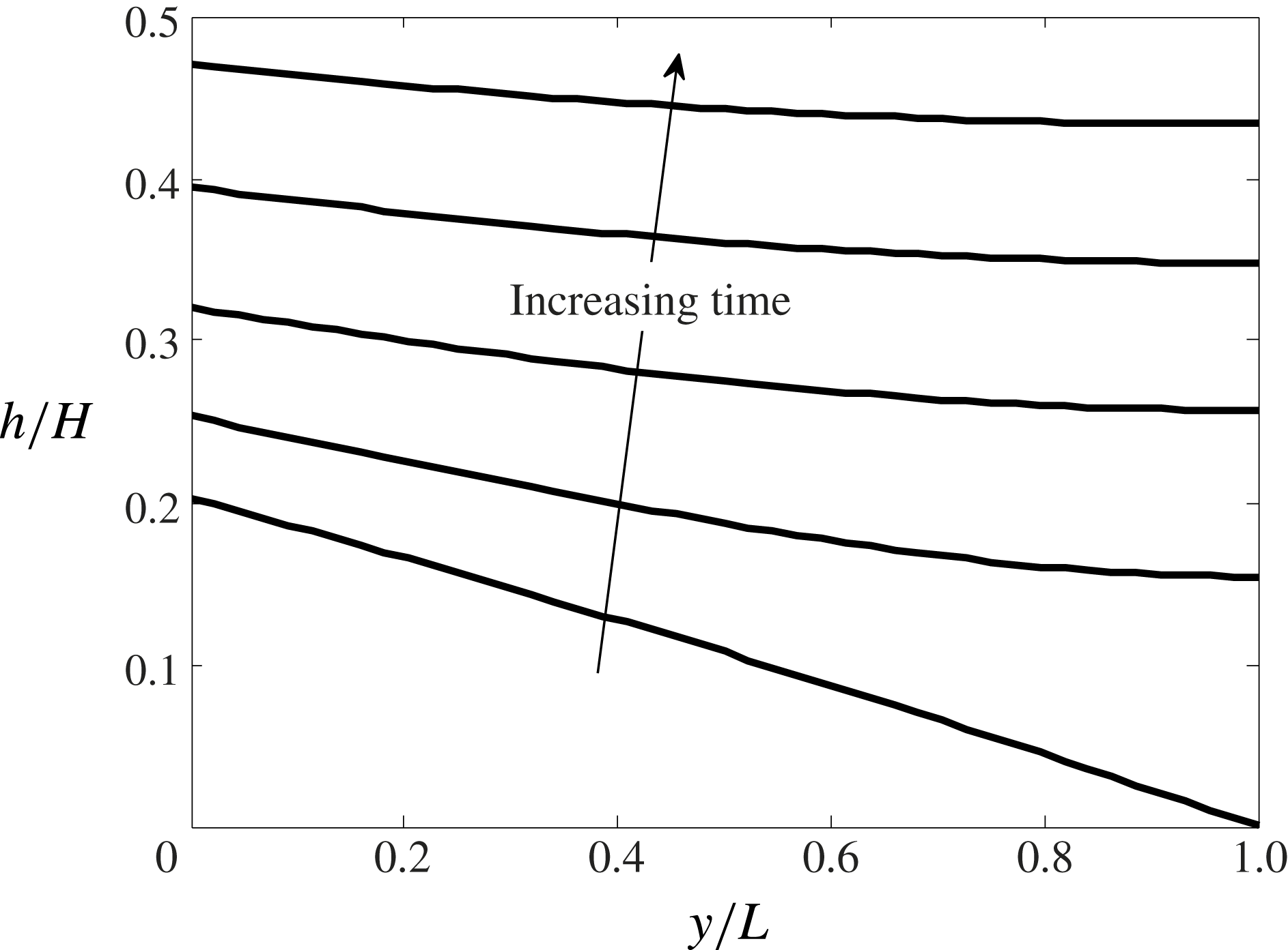
The numerical solution is then obtained using the methodology outlined in appendix A; sample results are given in figure 4.
Evolution of the first front. The non-dimensional time increment is
 $0.08t_{H}$
, starting with
 $t=t_{L}$
for the lowest curve. Note that
 $t_{H}$
is defined by (2.45). The values used for the numerical scheme are:
 ${\rm\Delta}y/L=10^{-3}$
,
 ${\rm\Delta}t/t_{H}=10^{-6}$
and
 $S=kg^{\prime }/{\it\phi}{\it\nu}=0.6~\text{cm}~\text{s}^{-1}$
, where
 ${\it\phi}=0.38$
.

As the first front advects upwards, its curvature diminishes in time, so that, as
 $t\rightarrow \infty$
, the boundary between discharged plume fluid and external ambient fluid becomes horizontal. The vertical advection of the first front can then be determined by simple volume flux balance, i.e.
 $$\begin{eqnarray}\lim _{t\rightarrow \infty }[{\it\phi}AU_{f}(h)]=\lim _{t\rightarrow \infty }[Q(x=H-h)],\end{eqnarray}$$
where
 $Q$
is defined by (2.24),
 $A$
is the control volume cross-sectional area, which is assumed to be both constant and much larger than that of the plume, and
 $U_{f}$
is the vertical velocity of the (horizontal) first front, which has an elevation of
 $h$
, i.e.
 $U_{f}(h)=\text{d}h/\text{d}t$
. Even before the long-time limit is realized, (2.42) can still be applied provided
 $h$
and
 $U_{f}$
are replaced by their
 $y$
-averaged mean values, i.e.
 $$\begin{eqnarray}{\it\phi}A\bar{U}_{f}(\bar{h})=Q(H-\bar{h}),\end{eqnarray}$$
where
 $\bar{U}_{f}(h)=\text{d}\bar{h}/\text{d}t$
. After applying (2.24), and with further integration and simplification, the predicted vertical distance,
 $\bar{h}_{2}-\bar{h}_{1}$
, travelled by the first front in time
 $t_{2}-t_{1}$
can be determined from
 $$\begin{eqnarray}\bar{h}_{2}=H+x_{0}-\left[(H+x_{0}-\bar{h}_{1})^{3/4}-\frac{3}{4}\frac{(t_{2}-t_{1})}{A}\left(\frac{16F_{0}k{\it\Lambda}{\it\alpha}^{1/2}}{{\rm\pi}{\it\nu}{\it\phi}^{3/2}}\right)^{1/2}\right]^{4/3}.\end{eqnarray}$$
By rearranging (2.44) and setting
 $\bar{h}_{2}=H+x_{0}$
and
 $\bar{h}_{1}=\bar{h}_{t_{L}}$
, we obtain the following characteristic time scale associated with the ascent of the first front from the bottom to the top of the control volume:
 $$\begin{eqnarray}t_{H}=\frac{4}{3}A\left(\frac{{\rm\pi}{\it\nu}{\it\phi}^{3/2}}{16F_{0}k{\it\Lambda}{\it\alpha}^{1/2}}\right)^{1/2}(H+x_{0}-\bar{h}_{t_{L}})^{3/4}.\end{eqnarray}$$
Qualitatively, this result is similar to equation (B3) of Caulfield & Woods (Reference Caulfield and Woods2002), who studied filling box flows for a control volume devoid of porous material and containing a free turbulent plume.
3. Laboratory set-up and experiments
Laboratory experiments were performed to verify select theoretical predictions from § 2. A transparent acrylic rectangular box 88.9 cm long
 $\times$
7.6 cm wide
 $\times$
50.8 cm tall was filled with tap water and Potters Industries A Series Premium glass beads. The beads were of uniform size, and had a diameter of either 0.3 cm or 0.5 cm and a density of
 $1.54~\text{g}~\text{cm}^{-3}$
as compared to
 $0.99~\text{g}~\text{cm}^{-3}$
for the tap water. We assume a porosity of
 ${\it\phi}=0.38$
for randomly distributed spherical beads (Happel & Brenner Reference Happel and Brenner1991).
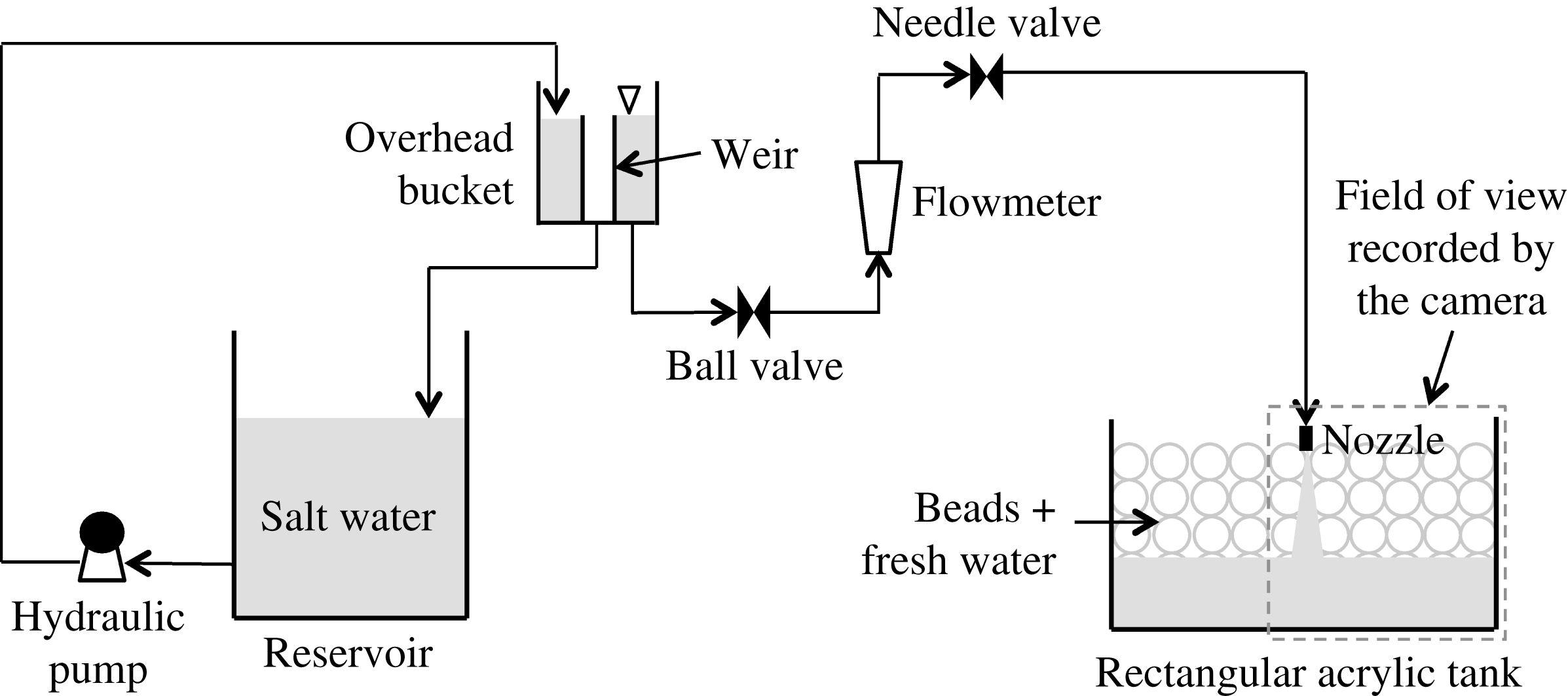
Schematic of the experimental set-up.

A schematic of the experimental set-up is shown in the figure 5. A specially designed line nozzle, manufactured to minimize the momentum of the source fluid by limiting the discharge velocity (Roes Reference Roes2014, appendix C.3), was used as the source and had a discharge area,
 $A_{\mathit{nozzle}}=2.8~\text{cm}^{2}$
. For simplicity, the nozzle, which spanned the width of the box, was positioned on-centre at
 $y=0$
. However, we expect that similar observations would have been recorded had the nozzle been located off-centre (but not too close to either sidewall). An overhead bucket was used for supplying dense fluid, which consisted of salt water dyed with Procion MX Cold Water dye. Dye was used for flow visualization purposes; its addition did not change the fluid density (
 ${<}1.10~\text{g}~\text{cm}^{-3}$
) or kinematic viscosity (
 $0.01~\text{cm}^{2}~\text{s}^{-1}$
). The overhead bucket contained a cylindrical internal weir to maintain a constant level. A Gilmont GV-2119-S-P flowmeter was used to measure the (time-invariant) source volume flux, which was set with the help of a ball valve and a needle valve. The overhead bucket was, in turn, supplied by a reservoir having a maximum capacity of 100 litres. Fluid densities were measured to an accuracy of
 $0.00005~\text{g}~\text{cm}^{-3}$
using an Anton Paar DMA 4500 density meter.
A Canon Rebel EOS T2i 18.0 PM camera with an 18–55 mm IS II zoom lens was used to capture experimental images, which were collected every 120 s. Thus, over the course a single experiment, which usually took approximately 3 h to complete, roughly 90 images were recorded. The camera was placed perpendicular to the front face of the acrylic tank, below which was located a mirror angled at 45° whose purpose was to provide details of the gravity current advance. The tank was backlit using a 3M 1880 overhead projector; to diffuse the light from this projector, a large sheet of white sketching paper was taped to the back of the tank. To minimize parallax effects, and also because of the symmetric nature of the flow, only one-half of the tank was in the field of view of the camera (figure 5).
All experimental images, including reference images that were recorded before the start of each experiment, were cropped to remove unwanted regions outside of the flow domain. Cropped images were then converted into grey scale and the reference image was subtracted to specifically highlight the descending plume, gravity current and ascending first front. Subtracted images were then divided into 20 vertical bands of equal width with bands 3–20 falling outside of the near-plume region. We used the post-processing algorithm described in Roes (Reference Roes2014) to estimate the interface height of the gravity current or first front in each of bands 3–20. Thus, in each band and for every time instant, pixels were first binned into
 $10\times 10$
boxes. Row-averaged pixel intensities were then calculated, which allowed us to compute the elevation corresponding to the maximum vertical intensity gradient. To improve upon this initial estimate for the interface height, data within
 $\pm 150$
pixels of the previously determined elevation were fitted using a high-order polynomial. Our refined estimate of the interface height was based on the vertical location corresponding to the maximum of the derivative of the polynomial. Thus we could measure the variation of the gravity current or first front interface height with
 $y$
or, by averaging over all 18 bands, compute the mean elevation over the width of the entire right-hand side of the tank.
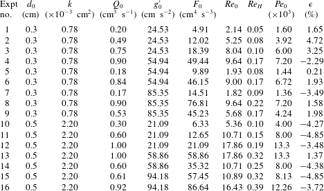
A list of the experiments performed is shown in appendix B, table 1. We regard the bead diameter
 $d_{0}$
, the plume source volume flux
 $Q_{0}$
and reduced gravity
 $g_{0}^{\prime }$
as independent variables. From these, the following derived variables were computed: the source buoyancy flux
 $F_{0}$
, Reynolds number
 $\mathit{Re}_{0}$
, Péclet number
 $\mathit{Pe}_{0}$
and the permeability
 $k$
of the porous medium. Note that
 $F_{0}=Q_{0}g_{0}^{\prime }$
. Moreover,
 $\mathit{Re}_{0}$
is given by
 $\mathit{Re}_{0}=Q_{0}d_{0}/(A_{\mathit{nozzle}}{\it\nu})$
. In the majority of experiments, the source Reynolds number was
 $\mathit{Re}_{0}\approx O(10)$
. (Note that
 $\mathit{Re}_{0}$
is the maximum value of the Reynolds number, which decreases with increasing
 $x$
as
 $\mathit{Re}\propto (x+x_{0})^{-1/4}$
.) In all cases, the source Péclet number is
 $\mathit{Pe}_{0}=Q_{0}d_{0}{\it\tau}/(A_{\mathit{nozzle}}D_{d})>100$
, where the molecular diffusion coefficient
 $D_{d}$
of the solute was estimated using the method suggested by Tyn and Calus – see (11-9.5) of Poling, Prausnitz & O’Connell (Reference Poling, Prausnitz and O’Connell2000) – and following Winsauer et al. (Reference Winsauer, Shearin, Masson and Williams1952) the tortuosity constant was assumed to be
 ${\it\tau}=2.0$
for
 ${\it\phi}=0.38$
. Furthermore, the permeability of the porous medium, corresponding to a medium comprising uniform spherical beads, is calculated based on the empirical relationship derived originally by Rumpf and Gupte, and subsequently applied by Acton, Huppert & Worster (Reference Acton, Huppert and Worster2001), Lyle et al. (Reference Lyle, Huppert, Hallworth, Bickle and Chadwick2005) and many others, such that
 $k={d_{0}}^{2}{\it\phi}^{5.5}/5.6$
.
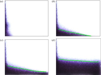
Plume, gravity current and curved interface experimental images. Images correspond to experiment 13 at (a)
 $t=0$
, (b)
 $t=0.7t_{L}$
, (c)
 $t=t_{L}+0.1t_{H}$
and (d)
 $t=t_{L}+0.3t_{H}$
, where
 $t_{L}$
and
 $t_{H}$
are defined by (2.36) and (2.45), respectively. The curves shown in (b–d) are the interface heights as computed using the MATLAB algorithm of § 3. The field of view for each image measures 44 cm long
 $\times$
36 cm tall.

4. Results and discussion
Illustrative experimental images are shown in figure 6. The curves on top of the laboratory images show the measured heights of the gravity current and first fronts. Figure 6(a) shows the time instant
 $t=0$
at which the descending plume, dyed purple, first reaches the impermeable bottom boundary. Thereafter, a rightward-propagating gravity current is formed, as exhibited in figure 6(b). Although our equations of § 2.2 assume a gravity current of a constant reduced gravity and corresponding gravity current density, we see in this experimental image evidence of a horizontal density gradient within the gravity current. By combining Darcy’s law, a hydrostatic pressure equation and Leibniz’s rule, it can be shown that this density gradient is dynamically insignificant provided
 $$\begin{eqnarray}\left|({\it\rho}-{\it\rho}_{0})\frac{\partial h}{\partial y}\right|\gg \left|\int _{0}^{h}\frac{\partial {\it\rho}}{\partial y}\,\text{d}(H-h)\right|.\end{eqnarray}$$
We assume that
 ${\it\rho}\propto I$
, where
 $I$
is the intensity of the false-colour grey scale laboratory images, and note that
 $I({\it\rho}={\it\rho}_{0})=0$
. Therefore, the condition to be satisfied becomes
 $$\begin{eqnarray}\left|I\frac{\partial h}{\partial y}\right|\gg \left|\int _{0}^{h}\frac{\partial I}{\partial y}\,\text{d}(H-h)\right|.\end{eqnarray}$$
A separate analysis, not presented here, confirms that the above inequality is satisfied in our experiments. Thus we conclude that the assumption made in deriving (2.28) is appropriate. Finally, figure 6(c–d) corresponds to times greater than
 $t_{L}$
. Discharged plume fluid accumulates in a deepening layer of contaminated fluid at the bottom of the control volume. Qualitatively, the shapes of the gravity current and of the first front are similar to the results displayed in figures 3 and 4, respectively. However, to make this comparison between the analytical predictions of § 2 and the experimental measurements of § 3 quantitatively meaningful, it is first necessary to estimate the numerical value of
 ${\it\alpha}$
, which first appears in (2.8) and reappears, for instance, in (2.24) and (2.44). For this purpose, we focus specifically on the long-time measurements of the first front elevation. (Note that, following the studies of free turbulent plumes (e.g. Baines & Turner Reference Baines and Turner1969), measuring the elevation of the first front is much more straightforward than trying to determine directly the plume volume flux and its variation with
 $x$
.) Using (2.42) as the reference analytical solution, the error-minimizing value of
 ${\it\alpha}$
is determined for each experiment. We then compute the average over all 16 experiments from table 1 of appendix B and find a mean value of
 ${\it\alpha}=0.015~\text{cm}$
. The mean errors presented in table 1 have standard and maximum deviations of
 $\pm 3\,\%$
and
 $\pm 5\,\%$
for the entire dataset. The small values just reported support the hypothesis that
 ${\it\alpha}=0.015~\text{cm}$
is a meaningful average value.
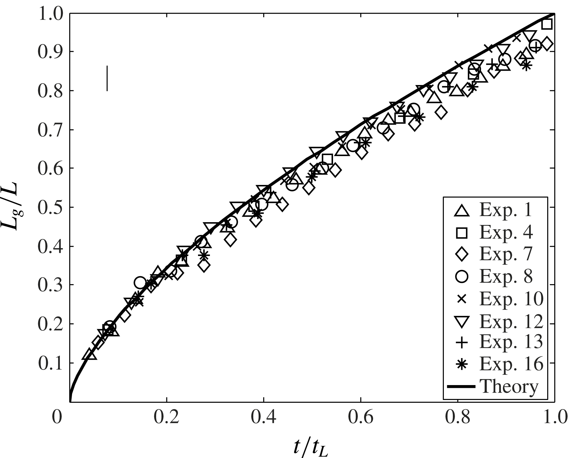
Gravity current front position versus time. A representative error bar is indicated in the upper left-hand side corner.

With this value for
 ${\it\alpha}$
to hand, separate comparisons can be made for the gravity current and first front problems. Starting with the gravity current, two different comparisons between theory and experiment are drawn: (i) the front position versus time,
 $t$
(figure 7), and (ii) the gravity current profile for various times (figure 8). In figure 7, the solid curve is adopted from (2.37). For clarity, we do not include the entirety of our experimental dataset but rather choose eight representative experiments from table 1 that span small and large
 $Q_{0}$
,
 $g_{0}^{\prime }$
and
 $d_{0}$
. Because the plume has a finite thickness when it reaches the bottom of the control volume at
 $t=0$
(see figure 6
a), the initial gravity current length is some finite value. Therefore measured values for
 $L_{g}$
are greater than zero when
 $t=0$
. To make a consistent comparison with the predictions of (2.37) for which
 $L_{g}=0$
when
 $t=0$
, it is therefore necessary to adjust the measured data so that the first data point of each set coincides with the solid curve. The meaningful comparison to be drawn between theory and experiment is therefore for intermediate and large values of
 $t$
; in the former case, good agreement is observed, whereas in the latter case predicted values for
 $L_{g}$
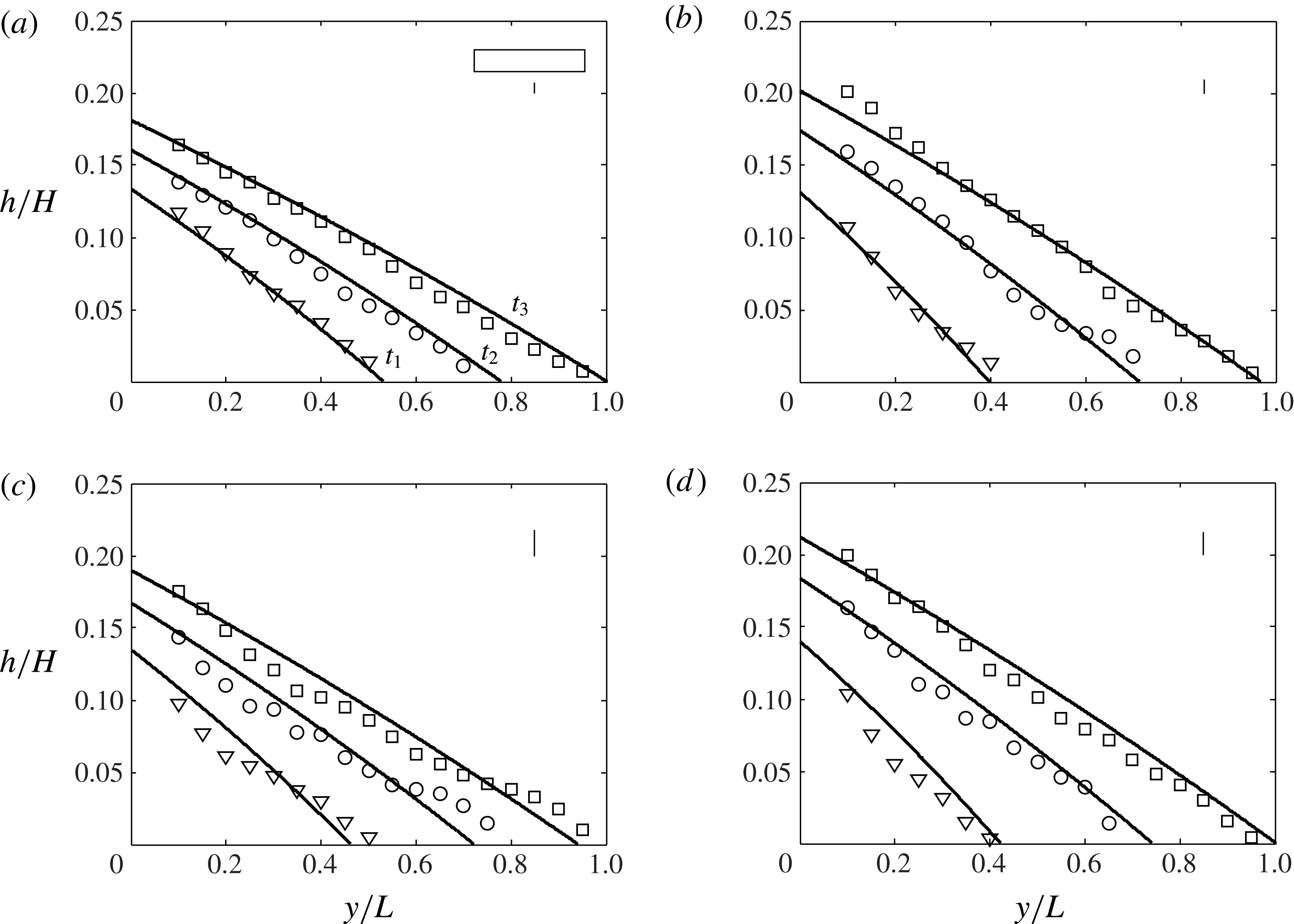
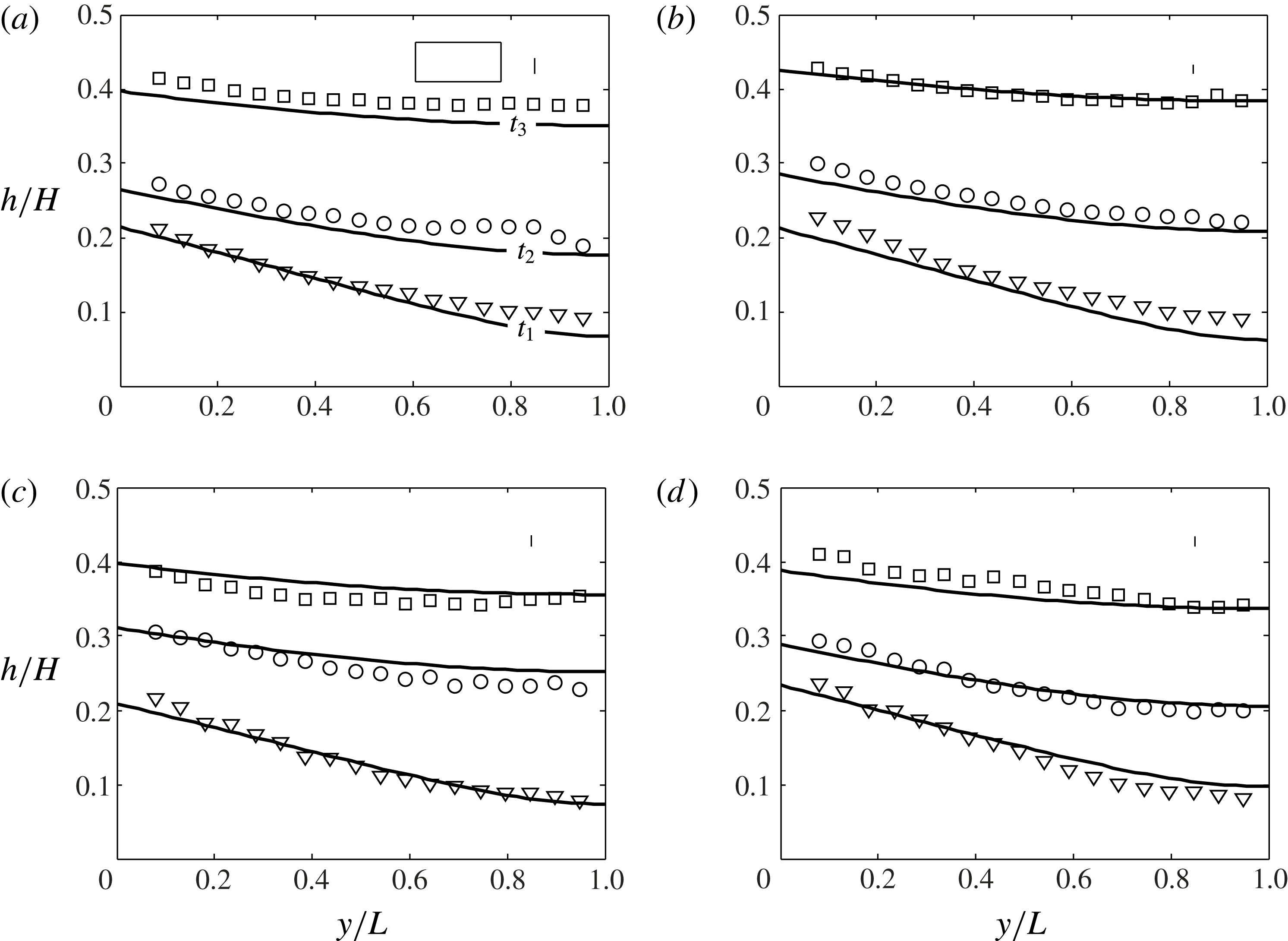
typically overpredict their measured counterparts. This observation is consistent with Huppert & Woods (Reference Huppert and Woods1995), who, in their investigation of a constant volume release in a Hele-Shaw cell, made similar observations and attributed their discrepancy to the influence of bottom friction near the front (see e.g. their figures 2 and 3). In figure 8, we show the gravity current profile at three distinct times for four different experiments. Experiments are chosen on the basis of their values for
 $F_{0}$
and
 $d_{0}$
, being in some instances comparatively small and in others comparatively large. In all cases, the measured heights show good agreement with the profiles predicted from (2.32). The positive comparisons drawn in figures 7 and 8 constitute an indirect validation for the computed value of
 ${\it\alpha}$
: the influx to the gravity current depends on
 $Q_{g}$
and
 $g_{g}^{\prime }$
, which are, in turn, functions of
 ${\it\alpha}$
as prescribed, for instance, by (2.24) and (2.25).
Gravity current profile: (a) experiment 1,
 $t_{1}=0.37t_{L}$
,
 $t_{2}=0.67t_{L}$
,
 $t_{3}=1.0t_{L}$
; (b) experiment 4,
 $t_{1}=0.25t_{L}$
,
 $t_{2}=0.60t_{L}$
,
 $t_{3}=0.95t_{L}$
; (c) experiment 10,
 $t_{1}=0.34t_{L}$
,
 $t_{2}=0.64t_{L}$
,
 $t_{3}=0.95t_{L}$
; and (d) experiment 13,
 $t_{1}=0.27t_{L}$
,
 $t_{2}=0.64t_{L}$
,
 $t_{3}=1.0t_{L}$
. The time scales
 $t_{L}$
and
 $t_{H}$
are defined by (2.36) and (2.45), respectively. Representative average error bars are indicated in the upper right-hand side corner of each panel. Also, a rectangle having unit aspect ratio in physical coordinates is indicated in (a).

In considering the first front, figure 9 compares the measured and predicted first front elevations for the same experiments, 1, 4, 10 and 13, as are considered in figure 7. In all cases, and consistent with figure 4, it is observed that the first front becomes more horizontal as
 $t$
increases. Equation (2.40) shows that the elevation,
 $h$
, of the first front depends upon the total volume,
 $V$
, of plume fluid discharged into the lower layer up until that particular instant in time. Hence the minor discrepancies observed in figure 9 are probably the result of differences in the values of the actual volume flux versus that estimated from (2.24).
Curved interface profile: (a) experiment 1,
 $t_{1}=t_{L}+0.04t_{H}$
,
 $t_{2}=t_{L}+0.08t_{H}$
,
 $t_{3}=t_{L}+0.13t_{H}$
; (b) experiment 4,
 $t_{1}=t_{L}+0.04t_{H}$
,
 $t_{2}=t_{L}+0.08t_{H}$
,
 $t_{3}=t_{L}+0.13t_{H}$
; (c) experiment 10,
 $t_{1}=t_{L}+0.03t_{H}$
,
 $t_{2}=t_{L}+0.09t_{H}$
,
 $t_{3}=t_{L}+0.14t_{H}$
; and (d) experiment 13,
 $t_{1}=t_{L}+0.04t_{H}$
,
 $t_{2}=t_{L}+0.07t_{H}$
,
 $t_{3}=t_{L}+0.11t_{H}$
. The time scales
 $t_{L}$
and
 $t_{H}$
are defined by (2.36) and (2.45), respectively. Representative average error bars are indicated in the upper right-hand side corner of each panel, and a rectangle having unit aspect ratio in physical coordinates is indicated in (a).

Furthermore, we can estimate the
 $y$
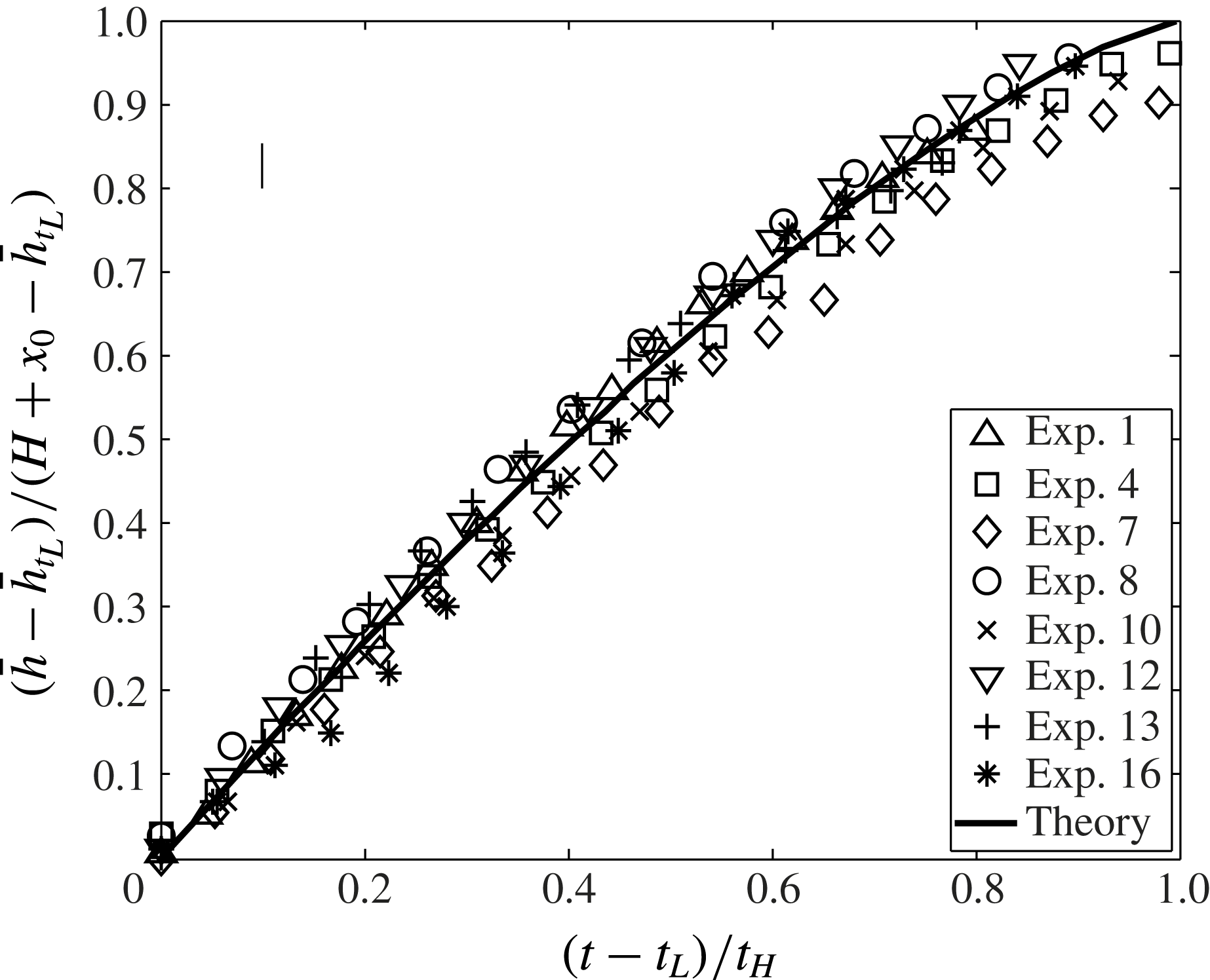
-averaged first front elevation versus time by adopting (2.44). Results are shown in figure 10, which includes the same set of representative experiments as in figure 7. We do not separately show the solution of (A 1) because this curve overlaps with the solid curve already present in figure 10. Elevations are non-dimensionalized by
 $H+x_{0}-\bar{h}_{t_{L}}$
, where
 $x_{0}$
is defined by (2.23) and
 $\bar{h}_{t_{L}}$
is defined by (2.38). Conversely, the abscissa is non-dimensionalized by
 $t_{H}$
, which is defined by (2.45). The overall comparison between theory and experiment is favourable. In particular, both suggest that the speed of ascent decreases as the first front approaches the source. This behaviour is qualitatively consistent with (2.24) and (2.43), the former of which indicates that the plume volume flux scales as
 $x^{1/4}$
.
First front elevation versus time. A representative error bar is indicated in the upper left-hand side corner.

We tried rationalizing the variation of the (non-dimensionalized) data by grouping our experimental measurements into different families according to the values of
 $g_{0}^{\prime }$
,
 $Q_{0}$
or
 $d_{0}$
. For better or worse, this analysis did not reveal any definitive trends other than that the first front elevation is moderately larger for small
 $Q_{0}$
– see figure 10. On this basis, we conclude that the non-dimensionalizations outlined above are appropriate in that they capture the leading-order physics of the flow.
A video comparing the numerical and experimental height profiles of the gravity current and first front for experiment 13 is included as electronic supplementary material (movie.mp4) available at http://dx.doi.org/10.1017/jfm.2015.555. The video is made in MATLAB by first combining 29 images, spaced at 20 s intervals where the horizontal and vertical axes are respectively normalized by
 $L$
and
 $H$
. Analogue numerical solutions are then superposed on top of the experimental images where we use the equations of §§ 2.2 and 2.3, respectively, when
 $t<t_{L}$
and
 $t>t_{L}$
.
5. Conclusions
Motivated by studies of filling box flows with turbulent free plumes (Baines & Turner Reference Baines and Turner1969), and based on previous investigations of laminar plumes (Wooding Reference Wooding1963; Roes et al.
Reference Roes, Bolster and Flynn2014) and gravity current flow (Huppert & Woods Reference Huppert and Woods1995) in porous media, a solution for filling box flows in the Darcy regime with
 $\mathit{Pe}\gg O(1)$
is derived. We assume a Boussinesq system where the dense and light fluids are fully miscible. The following three flow components are considered: (i) a (negatively buoyant) laminar plume, (ii) a pair of gravity currents comprising discharged plume fluid that propagate along the bottom of the control volume and (iii) the subsequent vertical advection of the discharged plume fluid towards the source.
In § 2.1, we derive a similarity solution for laminar plume flow. This solution assumes that molecular diffusion is negligible compared to mechanical dispersion,
 $D$
, and so applies in the ‘inner’ region close to the plume axis where flow speeds are comparatively large. In the context of (1.1), we assume that
 $\mathit{Pe}\gg O(1)$
. The solution is derived by employing a transverse dispersivity constant,
 ${\it\alpha}$
, in the governing equation (2.11) whose value, 0.015 cm, is determined by comparison with experimental measurements. In the inner region, variables such as the fluid density and vertical velocity change rapidly in the horizontal direction,
 $y$
, so that a Wooding-type boundary layer approximation can be applied in deriving the self-similar solution. In the outer region, by contrast, we assume that the vertical velocity and density perturbation are both zero. Our solution is therefore qualitatively similar to the ‘top hat’ description of turbulent free plumes, first proposed by Morton et al. (Reference Morton, Taylor and Turner1956), where molecular diffusion is likewise ignored.
The self-similar solution allows us to compute the plume volume flux,
 $Q$
, and mean reduced gravity,
 $\bar{g^{\prime }}$
, as functions of
 $x$
, the vertical coordinate. Indeed (2.24) and (2.25) respectively indicate that
 $Q$
and
 $\bar{g}^{\prime }$
are proportional to
 $x^{1/4}$
and
 $x^{-1/4}$
, contrary to the scalings
 $x^{1/3}$
and
 $x^{-1/3}$
that apply when
 $\mathit{Pe}\lesssim O(1)$
(Wooding Reference Wooding1963; Roes et al.
Reference Roes, Bolster and Flynn2014). The values of
 $Q$
and
 $\bar{g}^{\prime }$
calculated at the bottom of the control volume comprise the source conditions for the pair of gravity currents that are formed when the plume encounters the impermeable bottom boundary. The equations governing porous media gravity current flow are reviewed in § 2.2. In particular, the self-similar ODE (2.33), originally derived by Huppert & Woods (Reference Huppert and Woods1995) for (hydrostatic) gravity current flow and based on Darcy’s law (2.28) and a volume conservation equation (2.29), describes the variation of the gravity current height in space and time. The self-similar ODE (2.33), and associated boundary conditions (2.34), is solved by employing a shooting method to draw curves such as those shown in figure 3. Once the gravity current reaches the (impermeable) vertical sidewall of the control volume at
 $t=t_{L}$
, the motion becomes primarily vertical. The solution describing the motion of the first front, the interface separating the discharged plume fluid from the overlying ambient fluid, is presented in § 2.3. Similar to the gravity current problem, the equation that describes the spatio-temporal evolution of the first front, (2.41), is also based on Darcy’s law and a volume conservation equation. However, in this case no self-similar solution is possible and hence a finite difference numerical method is applied instead. Figure 4 indicates that the first front, whose initial shape matches that of the gravity current at
 $t=t_{L}$
, becomes progressively more horizontal with time so that, in the large-
 $t$
limit, the first front moves only vertically. Moreover, the advection speed of the first front decreases as it moves towards the plume source.
To verify key model predictions, complementary experiments are performed using fresh water and salt water as the working fluids. Particular emphasis is placed on the motion of the gravity current and of the first front, both of which depend on
 $Q$
and
 $\bar{g^{\prime }}$
. A comparison between theory and experiment is given in § 4. Figures 7 and 8 show, respectively, the gravity current front position,
 $L_{g}$
, versus
 $t$
, and the gravity current height,
 $h$
, versus
 $y$
at three different instants in time. Conversely figure 9 shows the shape of the first front, again for three different values of
 $t$
. Finally, figure 10 presents the time variation of the average first front elevation,
 $\bar{h}$
. In all cases, the agreement between the predictions and the measurements is promising. Thus, the experimental measurements provide support for the functional form of our plume solution according to which
 $Q\propto x^{1/4}$
.
By necessity, the present research is conducted using a set of limiting assumptions: the medium is isotropic, the fluids are miscible and the flow is both Boussinesq and of Darcy type. In many geological scenarios of interest, however, other factors, e.g. surface tension and anisotropy, may be relevant. In future research, the most restrictive of our assumptions will be relaxed by studying filling box flow in media characterized by spatially variable
 ${\it\phi}$
and
 $k$
. Further extensions of the research could include an examination of non-Boussinesq and/or non-Darcy flow.
Acknowledgements
The current research is supported by NSERC (Discovery Grant and RTI programmes) and Carbon Management Canada. The authors acknowledge the kind assistance provided by M. Roes in setting up the experiment and in writing the image post-processing algorithms used in extracting the data shown in figures 8–10. The authors also wish to thank S. Dalal for fruitful discussions concerning the numerical schemes described in § 2.3. Experiments were conducted in the laboratory of Dr B. R. Sutherland.
Supplementary movie
Supplementary movie is available at http://dx.doi.org/10.1017/jfm.2015.555.
Appendix A. Curved interface methodology
In this appendix, we present the details of the numerical technique employed to solve for the motion of the (curved) first front.
Space and time derivatives are discretized so that (2.41) is replaced by
 $$\begin{eqnarray}\frac{h_{i}^{n+1}-h_{i}^{n}}{{\rm\Delta}t}=\frac{S}{2{\rm\Delta}y^{2}}(h_{i-1}^{n+1}h_{i-1}^{n}-2h_{i}^{n+1}h_{i}^{n}+h_{i+1}^{n+1}h_{i+1}^{n}),\end{eqnarray}$$
where
 $i$
and
 $n$
represent space and time indices, respectively. By symmetry, we only concern ourselves with the right-hand side of the control volume so that
 $i=1$
corresponds to the box centreline at
 $y=0$
whereas
 $i=L/{\rm\Delta}y+1=I+1$
corresponds to the position of the right sidewall at
 $y=L$
. On further simplification and rearranging, (A 1) becomes,
 $$\begin{eqnarray}-\!(Rh_{i-1}^{n})h_{i-1}^{n+1}+(1+2Rh_{i}^{n})h_{i}^{n+1}-(Rh_{i+1}^{n})h_{i+1}^{n+1}=h_{i}^{n},\end{eqnarray}$$
where
 $R=S{\rm\Delta}t/(2{\rm\Delta}y^{2})$
. In matrix form, (A 2) is expressed as
 $$\begin{eqnarray}\left[\begin{array}{@{}cccccc@{}}1+2Rh_{2}^{n} & -Rh_{3}^{n} & 0 & 0 & \ldots & 0\\ -Rh_{2}^{n} & 1+2Rh_{3}^{n} & -Rh_{4}^{n} & 0 & \ldots & 0\\ & & & \ddots & & \\ 0 & \ldots & 0 & -Rh_{I-1}^{n} & 1+2Rh_{I}^{n} & -Rh_{I+1}^{n}\\ 0 & \ldots & 0 & 0 & -2Rh_{I}^{n} & 1+2Rh_{I+1}^{n}\end{array}\right]\left[\begin{array}{@{}c@{}}h_{2}^{n+1}\\ h_{3}^{n+1}\\ h_{4}^{n+1}\\ \vdots \\ h_{I-1}^{n+1}\\ h_{I}^{n+1}\\ h_{I+1}^{n+1}\end{array}\right]=\left[\begin{array}{@{}c@{}}h_{2}^{n}+Rh_{1}^{n}h_{1}^{n+1}\\ h_{3}^{n}\\ h_{4}^{n}\\ \vdots \\ h_{I-1}^{n}\\ h_{I}^{n}\\ h_{I+1}^{n}\end{array}\right].\vphantom{\mathop{\sum }_{\mathop{\sum }_{\sum }}}\end{eqnarray}$$
The additional factor of 2 that appears in matrix entry
 $(I,I-1)$
is due to the application of a ‘ghost point’ (Causon & Mingham Reference Causon and Mingham2010), which is required because of the no-flux boundary condition at the sidewalls, i.e.
 $\partial h/\partial y=0$
when
 $y=\pm L$
.
Equation (A 3) is solved using a shooting method. Thus an initial guess is provided for
 $h_{1}^{n+1}$
, whose value is refined through iteration whilst enforcing volume conservation via (2.40) (Causon & Mingham Reference Causon and Mingham2010). The discrete form of (2.40) reads
 $$\begin{eqnarray}{\it\phi}{\rm\Delta}y\mathop{\sum }_{i=1}^{I}\left[\frac{(h_{i+1}^{n+1}+h_{i}^{n+1})}{2}-\frac{(h_{i+1}^{n}+h_{i}^{n})}{2}\right]=Q_{g}(H-h_{1}^{n}){\rm\Delta}t.\end{eqnarray}$$
The left-hand side of (A 4), discretized in space, represents the volume displaced by the advancing first front over time
 ${\rm\Delta}t$
, whereas the right-hand side of the equation, discretized in time, represents the volume of discharged plume fluid supplied over the same time interval.
Appendix B. Experimental details
Table 1 provides the details of the experiments described in § 3. Parameters such as
 $F_{0}$
,
 $\mathit{Re}_{0}$
and
 $\mathit{Pe}_{0}$
are defined previously, whereas
 $\mathit{Re}_{H}$
, the plume Reynolds number at the bottom of the control volume, is estimated from
 $$\begin{eqnarray}\mathit{Re}_{H}=\frac{U(H)d_{0}}{{\it\nu}}=\left[\left(\frac{4F_{0}k}{{\rm\pi}^{3}{\it\nu}^{3}{\it\Lambda}}\right)^{2}\frac{{\it\alpha}^{3}}{{\it\phi}(H+x_{0})}\right]^{1/4}.\end{eqnarray}$$
The velocity
 $U(x)={\it\alpha}u(x)/d_{0}$
is a characteristic velocity where the transport velocity
 $u(x)$
is calculated by dividing the plume volume flux by its cross-sectional area. Thus,
 $$\begin{eqnarray}U(x)=\frac{{\it\alpha}}{d_{0}}\frac{Q(x)}{{\it\Lambda}[y({\it\eta}={\rm\pi})-y({\it\eta}=-{\rm\pi})]}.\end{eqnarray}$$
Finally the error,
 ${\it\epsilon}$
, is calculated via
 $$\begin{eqnarray}{\it\epsilon}=\frac{100\,\%}{N}\left(\mathop{\sum }_{1}^{N}\frac{\bar{h}_{ex}-\bar{h}_{th}}{\bar{h}_{ex}}\right),\end{eqnarray}$$
where
 $N$
is the number of experimental images collected (typically 60) and
 $\bar{h}_{ex}$
and
 $\bar{h}_{th}$
are the time-dependent measured and predicted first front heights. The value of
 $\bar{h}_{th}$
, determined from (2.44), directly depends upon the plume volume flux,
 $Q$
. Therefore, it is understood that the value of
 ${\it\epsilon}$
obtained using (B 3) incorporates the deviation of the theoretically predicted volume flux from its corresponding experimental value.
A summary of the experimental parameters: bead diameter
 $d_{0}$
, permeability
 $k$
, source volume flux
 $Q_{0}$
, source reduced gravity
 $g_{0}^{\prime }$
, source buoyancy flux
 $F_{0}$
, source Reynolds number
 $\mathit{Re}_{0}$
, plume Reynolds number at the bottom boundary
 $\mathit{Re}_{H}$
(defined in (B 1)), source Péclet number
 $\mathit{Pe}_{0}$
, and the mean error
 ${\it\epsilon}$
(defined in (B 3)).