1 Introduction
The processes involved in the interaction of propagating electron beams with background plasmas has been of long-standing astrophysical interest due to their close association with some of the most energetic solar system radio emissions, including Type III solar radio busts. The generally accepted explanation for Type III emission, the so-called plasma emission mechanism, is a long-standing, multiple-stage model which has been considered extensively by numerous authors who have refined the initial ideas of Ginzburg & Zhelezniakov (Reference Ginzburg and Zhelezniakov1958) (although it should be noted other possibilities exist, e.g. such as the linear mode conversion suggested by Forslund et al. Reference Forslund, Kindel, Lee, Lindman and Morse1975; Kim, Cairns & Robinson Reference Kim, Cairns and Robinson2007). In the first stage of the plasma emission model, electron beams which are injected in the low corona are susceptible to the bump-in-tail instability as they propagate through the background plasma, and thus the beams can generate Langmuir waves. In later stages, these beam-generated Langmuir waves are susceptible to nonlinear decay and three-wave interaction processes which go on to produce the electromagnetic emission. Whilst the theoretical specifics of the later stages vary (see the recent review of Reid & Ratcliffe Reference Reid and Ratcliffe2014 and references therein), for the purposes of this paper it is sufficient to understand that the initial stage – the production of a population of Langmuir waves due to a resonant interaction with the beam electrons – is a common feature of all such models.
The most basic treatment of this stage (the beam–plasma instability) is the application of quasi-linear theory (QLT) under the assumption of a homogeneous plasma, which describes the exchange of energy from diffuse, fast beam electrons into Langmuir waves at the resonant phase velocity (inverse Landau damping). Once the particles reach a plateau-type distribution, further wave growth is prohibited, due to the absence of a positive slope in the velocity distribution, and thus the instability is saturated. Under homogeneous QLT, the calculated saturation time implies a flight distance of beams originating in the corona of only hundreds of kilometres before reaching saturation (e.g. Sturrock Reference Sturrock1964). This is at odds with in situ solar wind measurements taken as far out as 1 AU, which have documented both the presence of bump-in-tail-type electron distributions and growth of Langmuir waves in excess of background levels (see e.g. Anderson et al. Reference Anderson, Eastman, Gurnett, Frank and Parks1981; Lin et al. Reference Lin, Potter, Gurnett and Scarf1981). Furthermore, simple homogeneous QLT models are unable to account for the observed spatial clumping of Langmuir waveforms in the solar wind (e.g. Gurnett et al. Reference Gurnett, Anderson, Scarf and Kurth1978); the explanation of which must appeal to other processes, such as the kinetic localisation process described by Muschietti, Roth & Ergun (Reference Muschietti, Roth and Ergun1995, Reference Muschietti, Roth and Ergun1996) by which the beam tends to spatially localise in a homogeneous medium as a result of nonlinearities in wave–particle resonances. Alternatively, localisations can also be produced directly as a result of background inhomogeneity, which we will explore in this paper.
Accounting for the presence of the density inhomogeneity in the background plasma has been shown in numerous studies to be a plausible explanation for the above discrepancies. Ryutov (Reference Ryutov1969), Breizman & Ryutov (Reference Breizman and Ryutov1970) and Nishikawa & Ryutov (Reference Nishikawa and Ryutov1976) considered the quasi-linear relaxation of an electron beam in the presence of density inhomogeneities. They found that due to presence of the density inhomogeneities, a de-resonation of the beam–particles and background wave field may occur, which impacts upon the efficacy of the beam relaxation. This broadening of resonances was found to be able to access both lower and higher velocities, and thus the formation of a high-energy tail in the beam velocity distribution function via a re-absorption of Langmuir wave energy was also predicted. The governing equations of Ryutov (Reference Ryutov1969) where also revisited by Voshchepynets & Krasnoselskikh (Reference Voshchepynets and Krasnoselskikh2013), who considered numerical solutions in order to relax assumptions about beam temperature used in the earlier analytical solutions.
A number of recent studies have attempted to simulate beam relaxation under realistic solar wind conditions in which the conclusions of Ryutov (Reference Ryutov1969) and Breizman & Ryutov (Reference Breizman and Ryutov1970) are thought to hold, in order to determine if such a system can account for the aforementioned observational discrepancies. Krafft, Volokitin & Krasnoselskikh (Reference Krafft, Volokitin and Krasnoselskikh2013, Reference Krafft, Volokitin and Krasnoselskikh2015), Krafft et al. (Reference Krafft, Volokitin, Krasnoselskikh and de Wit2014) have used numerical models based on a Hamiltonian approach whereby the dynamics of the background plasma particles, Langmuir and ion-acoustic wave fields are described by the Zakharov equations, which are coupled to a population of resonant beam–particles that are evolved according to a particle approach.
Krafft et al. (Reference Krafft, Volokitin and Krasnoselskikh2013) found that the plasma inhomogeneities crucially influence the characteristics of the Langmuir turbulence and the beam–plasma interaction. It was shown that the Langmuir wave growth becomes localized and clumpy, similar to recent observations by STEREO and other satellites. In their model beam particles quickly de-resonate from the Langmuir waves and mutual energy exchange between the two is hampered much faster than in the homogeneous plasma case. Krafft et al. (Reference Krafft, Volokitin and Krasnoselskikh2013) also found that a tail of accelerated electrons was formed and the velocities can exceed significantly the beam drift velocity, reaching two times the initial beam drift speed. Krafft et al. (Reference Krafft, Volokitin, Krasnoselskikh and de Wit2014, Reference Krafft, Volokitin and Krasnoselskikh2015) extended the work, constructing observable waveforms and considering the interplay with nonlinear wave–wave interaction processes respectively. Similarly, Voshchepynets et al. (Reference Voshchepynets, Krasnoselskikh, Artemyev and Volokitin2015), Voshchepynets & Krasnoselskikh (Reference Voshchepynets and Krasnoselskikh2015) have considered the specific influence of density inhomogeneities instead using a probabilistic model. They found that for the very rapid beams with beam velocity exceeding the electron thermal speed by a factor of 15, the relaxation process consists of two well-separated steps. In the first step, the major relaxation process occurs with the wave growth rate everywhere becoming almost close to zero or negative. In the second stage the system remains in the state close to state of marginal stability long enough to explain how the beam may be preserved travelling distances over 1 AU while still being able to generate the Langmuir waves that are usually detected in situ by satellites.
In light of these recent results there is a growing consensus that inhomogeneity will significantly modify the beam–plasma system and so cannot be ignored in the context of electron beams propagating in the solar wind. However, the changes to the relaxation of electron beams due to plasma inhomogeneity are yet to be considered using a fully kinetic approach. There are a two main motivations for considering the problem within a fully kinetic particle-in-cell (PIC) approach. Firstly, the PIC description of plasmas is in principle the most generalised approach and can describe a richer physical picture (theoretically containing all of the physics, in the limit of realistic numbers of particles). Secondly, the use of beam-only kinetics imposes an upper limit on excitable wave vectors as the beam relaxes towards smaller velocities during the velocity-space plateau formation. Thus, we note that the fully kinetic PIC simulation has the advantage of accessing the full
 $k$
-range. In this paper we therefore present the results of the first such study whereby an electron beam’s interaction with an inhomogeneous background is simulated using the fully kinetic particle-in-cell method.
The paper is structured as follows: in § 2 we describe the parameters used in our simulations. In § 3.1 we present the results for the homogeneous experiment, followed by the results of the different inhomogeneous results in § 3.2. The implications of the results are discussed in § 4, and conclusions are drawn in § 5.
2 Numerical set-up
In this paper we present the results of six numerical experiments in which a bump-in-tail unstable electron beam is initialized in the presence of a Maxwellian background which is increasingly irregular in space. The simulations are carried out in a one-dimensional (1-D) geometry using EPOCH, an open-source multidimensional particle-in-cell code. Full details of the underlying solver, along with benchmarking on test problems, are available in Arber et al. (Reference Arber, Bennett, Brady, Lawrence-Douglas, Ramsay, Sircombe, Gillies, Evans, Schmitz and Bell2015).
All parameters except for those relating to the spatial profile of the background particles are common to all six experiments. The homogeneous background plasma parameters, upon which the density irregularities are then imposed, is chosen as follows: the homogeneous background number density
 $n_{0}=n_{e}=n_{i}=5\times 10^{6}~\text{m}^{-3}$
and background electron temperature
 $T_{e}=10~\text{eV}$
. The beam particles are initialised with a shifted Maxwellian profile, with density
 $n_{b}/n_{0}=2.5\times 10^{-4}$
, speed
 $v_{b}=14V_{th,e}$
and velocity spread of
 $\unicode[STIX]{x0394}v_{b}=0.08v_{b}$
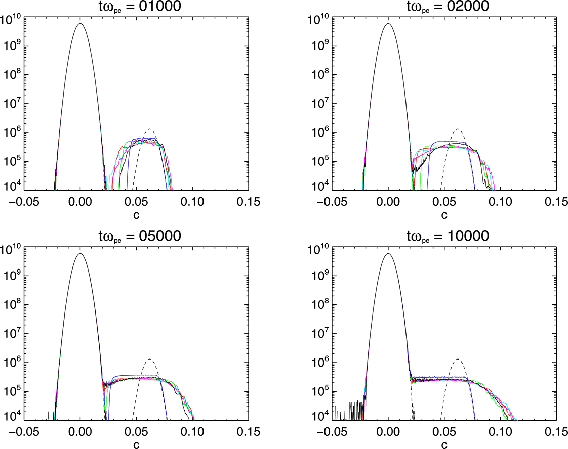
. The initial electron velocity distribution function may be seen in the dashed curves of figure 1.
Influence of the level of inhomogeneity on the evolution of the electron velocity distribution function with time, where
 $\unicode[STIX]{x0394}n=0$
(blue), 0.01 (green), 0.02 (red), 0.03 (cyan), 0.04 (magenta) and 0.05 (black). The initial profile of the electrons (common to all cases) is shown by the black dashed line.

The background density profile
 $n_{0}$
is modified from simulation-to-simulation with the addition of a spatially dependent perturbation
 $\unicode[STIX]{x1D6FF}n(x)$
such that
 $n_{0}^{\prime }(x)=n_{0}+\unicode[STIX]{x1D6FF}n(x)$
. The perturbation’s profile is comprised of ten harmonics:
 $$\begin{eqnarray}\unicode[STIX]{x1D6FF}n(x)=\frac{\unicode[STIX]{x0394}n}{N}\mathop{\sum }_{i=1}^{10}A_{i}\text{sin}\left(\frac{2\unicode[STIX]{x03C0}x+2\unicode[STIX]{x03C0}\unicode[STIX]{x1D719}_{i}}{\unicode[STIX]{x1D706}_{i}}\right).\end{eqnarray}$$
Each harmonic’s parameters were chosen randomly from a uniform distribution ranging from 0–1 (amplitude
 $A_{i}$
),
 $300\unicode[STIX]{x1D706}_{D}{-}2000\unicode[STIX]{x1D706}_{D}$
(wavelength
 $\unicode[STIX]{x1D706}_{i}$
) and 0–1 (phase-shift
 $\unicode[STIX]{x1D719}_{i}$
). The resulting signal was then normalised in amplitude by a factor
 $N$
that is calculated such that the average amplitude of the profile in question
 $\unicode[STIX]{x1D6FF}n(x)$
can be fixed by a choice of
 $\unicode[STIX]{x0394}n$
such that
 $\unicode[STIX]{x0394}n=\langle (\unicode[STIX]{x1D6FF}n/n_{0})^{2}\rangle ^{1/2}$
. Thus, the experiments considered vary as a choice of average profile percentage density fluctuation.
Following Ryutov (Reference Ryutov1969), the modified Langmuir wave dispersion relationship in the presence of such a density profile is to the first order
 $$\begin{eqnarray}\unicode[STIX]{x1D714}(k,x)\approx \unicode[STIX]{x1D714}_{pe}\left(1+\frac{1}{2}\frac{\unicode[STIX]{x1D6FF}n(x)}{n_{0}}\right)+\frac{3}{2}\frac{k^{2}V_{th,e}^{2}}{\unicode[STIX]{x1D714}_{pe}}.\end{eqnarray}$$
Where
 $\unicode[STIX]{x1D714}_{pe}$
is the electron plasma frequency and
 $V_{th,e}$
the electron thermal velocity. Thus, for density fluctuation to be large enough to cause beam Langmuir wave de-resonance we require the density ratio term on right-hand side of (2.2) to be larger than the third term. This yields
 $$\begin{eqnarray}\unicode[STIX]{x0394}n\geqslant 3\frac{k^{2}V_{th,e}^{2}}{\unicode[STIX]{x1D714}_{pe}^{2}}.\end{eqnarray}$$
Noting that the expected wavenumber associated with the two stream instability is approximately
 $k\approx \unicode[STIX]{x1D714}_{pe}/v_{b}$
then we deduce
 $$\begin{eqnarray}\unicode[STIX]{x0394}n\geqslant 3\left(\frac{V_{th,e}}{v_{b}}\right)^{2}.\end{eqnarray}$$
We therefore expect choices of average density profile satisfying (2.4) to act in the inhomogeneous regime described by Ryutov (Reference Ryutov1969). In this paper we present results for choices
 $\unicode[STIX]{x0394}n=0$
(a homogeneous plasma) and
 $\unicode[STIX]{x0394}n=0.01,0.02,\ldots ,0.05$
(inhomogeneous plasmas which are in excess of the threshold equation (2.4) as calculated for our parameter choices). The resulting density profiles for our specific choices of
 $\unicode[STIX]{x0394}n$
are illustrated later in figures 5, 9 and 10.
At this stage it is important to note two features of this profile. Firstly, we immobilise the ions and thus keep this profile fixed throughout the simulation. Thus, the ion-to-electron mass ratio is infinite and results are independent of the ion temperature. This is necessary in that it avoids the problem of the fluctuations subsiding due to kinetic damping in the absence of an external pump driving ion-acoustic turbulence, which in test runs was found to occur much more rapidly than the relaxation time of the instability (and so, otherwise mobile ions would prohibit the experiment). Secondly, it follows that the profile’s spatial scale is in fact fixed (the amplitude of each ‘potential well’ is a variable, however the length is fixed). This allows for direct comparisons regarding the specific influence of the amplitude as opposed to that of changing spatial scales which, according to inhomogeneous QLT, are also a factor in influencing the relaxation (see, e.g. Ryutov Reference Ryutov1969). The peak-to-peak spatial scales of the resulting density cavities (arising from our choice of constituent harmonics in (2.1)) are around
 $1000\unicode[STIX]{x1D706}_{D}$
, two orders of magnitude longer than the expected wavelengths excited by the beam–plasma interaction, which in this case is approximately
 $14\unicode[STIX]{x1D706}_{D}$
. Thus, this satisfies two (intuitive) scale requirements of the inhomogeneity; namely that scale should be larger than the Langmuir wavelengths so that the waves fit within the cavities, but be sufficiently short compared to the wave propagation scale (the product of their group speed and growth rate) such that the waves will experience refractive effects before the saturation of the instability (viz. the gradient is not too gentle). Such requirements are formally discussed by Ryutov (Reference Ryutov1969).
The chosen beam and (homogeneous) background parameters, except for the beam-to-background density ratio, are the same those used in the aforementioned Hamiltonian model of Krafft et al. (Reference Krafft, Volokitin and Krasnoselskikh2013). This choice is motivated by both suitability for solar wind plasmas and also to maximise comparability between the results. However, because the quasilinear instability time
 $\unicode[STIX]{x1D70F}_{ql}$
is known to scale as
 $\unicode[STIX]{x1D70F}_{ql}\unicode[STIX]{x1D714}_{pe}=(n_{b}/n_{0})^{-1}(v_{b}/\unicode[STIX]{x0394}v_{b})^{2}$
(see Melrose & McPhedran Reference Melrose and McPhedran1991), running a fully kinetic PIC code for a diffuse astrophysical beam (where
 $n_{b}/n_{0}\sim 10^{-6}$
, i.e. running for hundreds-of-thousands of plasma periods) with sufficient resolution and particle representation and time step (fractions of a plasma period) is unfeasible. As such, we have taken
 $n_{b}/n_{0}$
as an order of magnitude larger in order to be able to complete the simulations with the available computational resources. As discussed by Thurgood & Tsiklauri (Reference Thurgood and Tsiklauri2015), due to the beam–plasma system’s sensitive parameter space, this may compromise complete comparability.
The simulations are ran for
 $10^{4}$
plasma periods (
 $\unicode[STIX]{x1D714}_{pe}^{-1}$
) in a periodic domain of size
 $L_{x}=5000\unicode[STIX]{x1D706}_{D}$
with 5000 cells, thus grid is resolved to the Debye length
 $\unicode[STIX]{x0394}x=\unicode[STIX]{x1D706}_{D}$
and comfortably spans many individual cavities of the density profile. With a beam velocity of
 $v_{b}=14V_{th,e}$
, streaming beam electrons will cross the grid approximately 28 times during the simulation, crossing through many individual density cavities and being recycled through the boundaries. The expected group velocity of waves excited by the two stream instability is much slower – of order
 ${\sim}0.2V_{th,e}$
, and so (unmodified) propagating wave packets will travel distances of approximately
 $2000\unicode[STIX]{x1D706}_{D}$
, in excess of the cavity lengths, and so should experience the effects of the density gradient. The number of computational particles per cell per species (PPCPS) used is 5000 for background electrons and ions and 1315 PPCPS for the beam electrons. The cell-to-cell particle loading noise associated with the choice of 5000 PPCPS for the background has a root-mean-square fluctuation of approximately 0.3 %, an order of magnitude less than inhomogeneous density threshold (2.4). Thus, the inhomogeneous density profiles considered in this paper are clearly resolved against the noise. This particle resolution was the maximum given available resources, and as such we were unable to confidently separate intermediate profiles where
 $0<\unicode[STIX]{x0394}n<3(V_{th,e}v_{b}^{-1})^{2}$
from the noise levels – thus we do not consider the intermediate case of ‘weak inhomogeneity’ in this paper. Each run took approximately 72 h of run time on 128 cores (
 $8\times 2\times 8$
core Intel Xeon E5-2650 v2 processors).
3 Results
3.1 Homogeneous regime
We begin by describing the results of the homogeneous (
 $\unicode[STIX]{x0394}n=0$
) simulation before comparing with results for the inhomogeneous regime (where
 $\unicode[STIX]{x0394}n$
satisfies (2.4)) in § 3.2.
Figure 1 shows the evolution of the electron velocity distribution function of the six runs of increasing inhomogeneity
 $\unicode[STIX]{x0394}n=0,0.01,0.02,\ldots ,0.05$
at four instances in time (
 $t\unicode[STIX]{x1D714}_{pe}=1000,2000,5000,10\,000$
). Focusing on the
 $\unicode[STIX]{x0394}n=0$
case for now (blue curve) we see the saturation of the initial bump-in-tail instability and the merging of the beam electrons to the bulk distribution, resulting in the characteristic plateau formation. This is observed to occur by around
 $t\unicode[STIX]{x1D714}_{pe}=9000$
, which is in excess of the time scale predicted by the aforementioned quasi-linear theory formula (
 $\unicode[STIX]{x1D70F}_{ql}\unicode[STIX]{x1D714}_{pe}=(n_{b}/n_{0})^{-1}(v_{b}/\unicode[STIX]{x0394}v_{b})^{2}$
). We however, confirmed that this is a realistic relaxation time for this set-up in our convergence testing, rather than being artificially hastened as a side effect of poor computational particle counts as reported by Ratcliffe et al. (Reference Ratcliffe, Brady, Che Rozenan and Nakariakov2014) and Lotov et al. (Reference Lotov, Timofeev, Mesyats, Snytnikov and Vshivkov2015). The discrepancy is instead due to the use of the relatively dense and energetic beams which are outside of the formal applicability of the quasi-linear theory, as discussed in § 2. Furthermore, we note that there is no formation of a high-energy tail which is consistent with expectations of homogeneous quasi-linear theory. Ratcliffe et al. (Reference Ratcliffe, Brady, Che Rozenan and Nakariakov2014) and Lotov et al. (Reference Lotov, Timofeev, Mesyats, Snytnikov and Vshivkov2015) have both also noted that insufficient PPCPS leads to the erroneous formation of an unphysical high-energy tail. As such, this serves as confirmation that our PPCPS count is sufficient to correctly resolve the beam–plasma instability with no such numerical artefact. Given that there is no such artefact for
 $\unicode[STIX]{x0394}n=0$
, in § 3.2, when we consider inhomogeneous results, any sign of high-energy tail formation is therefore physically realistic.
The evolution of total field and particle energy is shown in figure 2 for the various simulations. For
 $\unicode[STIX]{x0394}n=0$
we see the instability onset at around
 $t\unicode[STIX]{x1D714}_{pe}=250$
which corresponds to a growth of electric field energy in (a) and a concomitant loss of particle energy in (b). The growth continues until the saturation time near
 $t\unicode[STIX]{x1D714}_{pe}=9000$
, which corresponds to the observed plateau formation time in figure 1. In (c), we see that the total simulation energy is well conserved to within
 ${<}0.002\,\%$
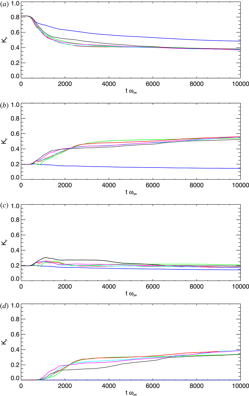
(for all of the simulations, i.e. numerical heating is negligible). Figure 3 more specifically shows the kinetic energy evolution of the population of beam particles, contained within different velocity ranges. Specifically, the four bands are (i)
 $K_{p}(v<v_{b}+\unicode[STIX]{x0394}v_{b})$
, (ii)
 $K_{p}(v>v_{b}+\unicode[STIX]{x0394}v_{b})$
, (iii)
 $K_{p}(v_{b}+\unicode[STIX]{x0394}v_{b}<v<v_{b}+3\unicode[STIX]{x0394}v_{b})$
and (iv)
 $K_{p}(v>v_{b}+3\unicode[STIX]{x0394}v_{b})$
. In the
 $\unicode[STIX]{x0394}n=0$
case (blue curve) we see that the beam has a net loss of kinetic energy across the different ranges, primarily from the main thermal bulk in range (i). There is no gain of kinetic energy in any range which is consistent with the absence of any high-energy tail formation for
 $\unicode[STIX]{x0394}n=0$
in figure 1.
Evolution of (a) total field energy (
 $J$
), (b) total particle energy (
 $J$
), and (c) total simulation energy (% change) over time for the six runs of increasing inhomogeneity amplitude –
 $\unicode[STIX]{x0394}n=0$
(blue), 0.01 (green), 0.02 (red), 0.03 (cyan), 0.04 (magenta) and 0.05 (black).

Evolution of the kinetic energy budget of the beam particles in four different velocity ranges for different values of
 $\unicode[STIX]{x0394}n$
, showing net acceleration and deceleration processes. The four velocity bands correspond to
 $K_{p}(v<v_{b}+\unicode[STIX]{x0394}v_{b})$
(a),
 $K_{p}(v>v_{b}+\unicode[STIX]{x0394}v_{b})$
(b),
 $K_{p}(v_{b}+\unicode[STIX]{x0394}v_{b}<v<v_{b}+3\unicode[STIX]{x0394}v_{b})$
(c) and
 $K_{p}(v>v_{b}+3\unicode[STIX]{x0394}v_{b})$
(d).
 $K_{p}$
is normalised by the initial kinetic energy of the beam. The level of inhomogeneity is indicated by line colour –
 $\unicode[STIX]{x0394}n=0$
(blue), 0.01 (green), 0.02 (red), 0.03 (cyan), 0.04 (magenta) and 0.05 (black).

We now turn our attention to the behaviour of the electrostatic waves generated by the beam relaxation. Figure 4 shows the evolution of electric field energy of the homogeneous simulation in
 $(k,\unicode[STIX]{x1D714})$
-space by considering 2-D, Fourier transforms in
 $(x,t)$
-space windowed over subsequent time periods. The time window size of
 $100\unicode[STIX]{x1D714}_{pe}^{-1}$
was determined by experimentation and provides the best balance between frequency resolution and effective time cadence, allowing us to track the evolution in both Fourier space and time, whilst preserving sufficient frequency resolution to reasonably compare spectra to expected dispersion curves. The decibel scale is defined with a reference (spectral) energy density level of 1, i.e. the plotted quantity is
 $10\log (0.5\unicode[STIX]{x1D716}_{0}{\mathcal{F}}(E_{x}(x,t))^{2})$
. The dispersion curves for the expected beam mode
 $\unicode[STIX]{x1D714}=v_{b}k$
and the (unmodified by the beam) Langmuir mode
 $\unicode[STIX]{x1D714}^{2}=\unicode[STIX]{x1D714}_{pe}^{2}+3k^{2}V_{th,e}^{2}$
are overlaid. We find that the majority of initial growth occurs on the intersection of the beam mode and Langmuir mode, i.e. the expected wave–particle resonance. As time advances, this spectral energy density shifts to the right of the intersection of the overlaid curves (i.e. the resonance shifts along the Langmuir dispersion curve towards higher
 $k$
). This is due to a dynamic shift in the resonance point as the instability proceeds – as beam particles loose energy and join the main population, the effective beam velocity is reduced and so the resonance point shifts along the Langmuir wave dispersion curve to higher
 $k$
. There is also some development of spectral energy density in the negative
 $k$
for the homogeneous case (see especially the blue curve in figure 8). This is a minor effect, barely noticeable in figure 4. We also note the presence of a spectral peak at the harmonic of the beam-driven waves, i.e. at
 $(2k_{L},\unicode[STIX]{x1D714}_{L})$
. This could be a signature of kinetic localisation as described by Muschietti et al. (Reference Muschietti, Roth and Ergun1995, Reference Muschietti, Roth and Ergun1996).
Embedded movie showing the evolution of time-windowed fast Fourier transforms of electric field energy in
 $(k,\unicode[STIX]{x1D714})$
-space for the homogeneous simulation.

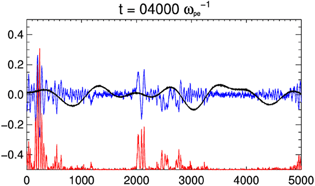
Embedded movie showing the wave packet evolution for
 $\unicode[STIX]{x0394}n=0$
. The blue curve shows the spatial profile of the electric field
 $E_{x}$
(
 $\text{V}~\text{m}^{-2}$
), the red shows
 $10E_{X}^{2}-0.5$
and the black shows the density profile
 $\unicode[STIX]{x1D6FF}n/n_{0}$
.

Finally, with regards to the spectra, we also note the presence of a small spectral peak at
 $k=0$
visible at early times. This is most clearly visible in figure 8, where the spectra of figure 4 and similar have been integrated over
 $\unicode[STIX]{x1D714}$
for direct comparison between different choices of
 $\unicode[STIX]{x0394}n$
(see § 3.2 for full details). Occurring for all values of
 $\unicode[STIX]{x0394}n$
, this corresponds to a beam-aligned, standing mode of the electric field
 $E_{x}$
oscillating at the local Langmuir frequency, which is present from the simulation initialisation (thus, before the instability onset). It is caused by the non-zero initial current imposed by the beam at
 $t=0$
, and has been discussed in detail by Baumgärtel (Reference Baumgärtel2013). Whilst it is possible to remove this mode by introducing a compensating drift velocity to the background electrons, we tolerate its presence as it is unclear whether such a compensation is physically appropriate (in particular, it may influence the correct return-current processes). Regardless, we have found that the amplitude associated with this mode, is in all runs much less than that of the Langmuir waves generated after the instability onset and as such it does not significantly affect the dynamics of the participating Langmuir wave population.
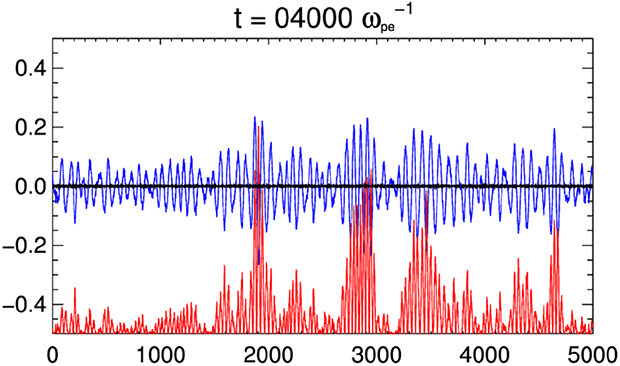
The time evolution of the generated electrostatic waves is presented in figure 5. In particular, it shows the evolution of the electric field in
 $(x,t)$
-space in the homogeneous case (blue curve), and a scaled measure of electric field energy density (
 $10E_{X}^{2}-0.5$
, red-curve). After the instability onset, a near-monochromatic wave, with a clear rightward-propagating character starts to grow. In the time interval
 $t\unicode[STIX]{x1D714}_{pe}=2000{-}4000$
, we note two effects in the homogeneous simulation – firstly, a coherent amplitude modulation due to the beating with the aforementioned standing oscillation of the electric field (see also Baumgärtel Reference Baumgärtel2013), and secondly, signs of amplitude localisation in
 $E_{x}$
, or ‘clumping’. The localisation in this case, given the absence of both density inhomogeneity and ion-acoustic participation (due to fixed ions), is due to the nonlinear kinetic localisation as described by Muschietti et al. (Reference Muschietti, Roth and Ergun1995, Reference Muschietti, Roth and Ergun1996), a process which is consistent also with the observation of the harmonic signal previously noted in the Fourier spectra.
3.2 Inhomogeneous regime and comparisons
We now turn our attention to the five simulations where the average density fluctuation is in excess of the quasi-homogeneous threshold equation (2.4), and consider how they differ from the homogeneous case considered in § 3.1. Returning to figure 1, we note that all of the inhomogeneous simulations differ from the homogeneous case in that (i) the deceleration of the bulk of the beams particles and associate plateau formation is enhanced and (ii) beam’s particles are also accelerated to higher velocities leading to the formation of a high-energy tail. Thus, we immediately see that there are two competing effects of the changes to wave–particle resonances due to the inhomogeneity, namely; (i) an enhanced deceleration process due to a broader range of available particle-to-wave resonances, and (ii) an acceleration process due to the re-absorption of wave-field energy into accelerated beam particles. The particular rates of these two process and the competition between them are found to vary in the inhomogeneous regime depending on the particular choice of
 $\unicode[STIX]{x0394}n$
. The difference is more clear in the evolution of energy budgets (such as overall wave and particle energies in figure 2, and the beam kinetic energy budgets in different velocity ranges in figure 3) and in the evolution of the wave-field spectrum (figures 6, 7, 9 and 10).
Embedded movie showing the evolution of time-windowed fast Fourier transforms of electric field energy in
 $(k,\unicode[STIX]{x1D714})$
-space for the
 $\unicode[STIX]{x0394}n=0.01$
simulation.

Embedded movie showing the evolution of time-windowed fast Fourier transforms of electric field energy in
 $(k,\unicode[STIX]{x1D714})$
-space for the
 $\unicode[STIX]{x0394}n=0.05$
simulation.

Comparison of
 $k$
-space evolution of electric field energy for different levels of inhomogeneity with time, where
 $\unicode[STIX]{x0394}n=0$
(blue), 0.01 (green), 0.02 (red), 0.03 (cyan), 0.04 (magenta) and 0.05 (black).

Embedded movie showing the wave packet evolution for
 $\unicode[STIX]{x0394}n=0.01$
. The blue curve shows the spatial profile of the electric field
 $E_{x}$
(
 $\text{V}~\text{m}^{-1}$
), the red shows
 $10E_{X}^{2}-0.5$
and the black shows the density profile
 $\unicode[STIX]{x1D6FF}n/n_{0}$
.

Embedded movie showing the wave packet evolution for
 $\unicode[STIX]{x0394}n=0.05$
. The blue curve shows the spatial profile of the electric field
 $E_{x}$
(
 $\text{V}~\text{m}^{-1}$
), the red shows
 $10E_{X}^{2}-0.5$
and the black shows the density profile
 $\unicode[STIX]{x1D6FF}n/n_{0}$
.

First considering the overall particle and wave energy as per figure 2, we see that in all inhomogeneous cases considered the net effect of the resonance broadening has been to significantly curtail the maximum level of gained by the waves (a), and thus lost by the particles (b). In comparison to the homogeneous case, the peak total wave-field energy is in the range
 $(5{-}10)\times 10^{-10}~\text{J}$
. This is approximately 2–4 times less than the homogeneous case, which peaks at approximately
 $1.9\times 10^{-9}~\text{J}$
. The peak wave energies (or minimum particle energies) are, in all cases, reached at earlier times than in the homogeneous case and so the overall instability time scale has been reduced (which is consistent with the more rapid plateau formation visible in figure 1). The initial growth rates leading to the maxima/minima of wave/particle energy are found to vary depending on the choice of
 $\unicode[STIX]{x0394}n$
. For
 $\unicode[STIX]{x0394}n=0.01$
, 0.02 and 0.03 growth rates are actually initially slightly faster than the homogeneous rate, for
 $\unicode[STIX]{x0394}n=0.04$
the growth rate is approximately the same as the homogeneous rate, and only for
 $\unicode[STIX]{x0394}n=0.05$
we see a comparatively slower growth rate. This pattern is also seen in the overall value of the maxima/minimum wave/particle energies – within the class of inhomogeneous runs,
 $\unicode[STIX]{x0394}n=0.01$
, 0.02 and 0.03 achieve the highest amount of wave-particle energy exchange, whereas
 $\unicode[STIX]{x0394}n=0.04$
and
 $\unicode[STIX]{x0394}n=0.05$
achieve less. Following the peak/minimum wave/particle energy, the dominant energy exchange process is reversed and so the wave fields have a net loss of energy to the particles, which appears to asymptotically tend to the same value for all choices of
 $\unicode[STIX]{x0394}n>0$
. This is consistent with the end-state velocity distribution function in figure 1, whereby all inhomogeneous runs have approximately the same phase-space profile at
 $t\unicode[STIX]{x1D714}_{pe}=10\,000$
.
Returning to figure 3, we now compare the results in terms of the evolution of the kinetic energy distribution of the beam particles. The overall trend for the inhomogeneous runs is consistent with our description of figures 1 and 2 – compared to the
 $\unicode[STIX]{x0394}n=0$
run we see a enhanced deceleration of the thermal beam electrons (a, where
 $K_{p}(v<v_{b}+\unicode[STIX]{x0394}v_{b})$
). Not only is this a more rapid deceleration, but it is continuous for sufficiently long to reach a greater level of depletion, with less kinetic energy being contained within the plateau at end times. However, this is superficially inconsistent with what we have seen with figure 2, whereby the
 $\unicode[STIX]{x0394}n>0$
cases retain more overall particle energy and transfer less overall energy to the Langmuir waves. The resolution is, of course, in that the enhanced energy loss due to deceleration is adequately compensated by the acceleration associated with the high-energy tail formation, where we see a growth of kinetic energy associated with particles in excess of the beam’s thermal range ((b), where
 $K_{p}(v>v_{b}+\unicode[STIX]{x0394}v_{b})$
). By late times, the combined net effect of the deceleration and acceleration processes is such that the beam kinetic energy for
 $\unicode[STIX]{x0394}n>0$
is in the range
 $0.87{-}0.88K_{p}(t=0)$
, far in excess of the
 $\unicode[STIX]{x0394}n=0$
case where it is approximately
 $0.64K_{p}(t=0)$
. Thus, in the inhomogeneous case, we see that the beams loose less overall energy to the background wave field. All choices of
 $\unicode[STIX]{x0394}n>0$
have a similar end state in the thermal range (a), which is consistent with the observation of figure 1 that all inhomogeneous runs considered appear to tend towards the same plateau shape, height and extent. For higher choices of inhomogeneity
 $\unicode[STIX]{x0394}n=0.04$
and 0.05, we see in (b) that the acceleration process has an earlier onset, specifically from the range (iii). Interestingly, it appears that by the end state, the acceleration to the largest velocities (c,
 $K_{p}(v>v_{b}+3\unicode[STIX]{x0394}v_{b})$
) is less efficient for the
 $\unicode[STIX]{x0394}n=0.01$
and 0.05 runs than the
 $\unicode[STIX]{x0394}n=0.02$
, 0.03, 0.04 runs, suggesting that this process may not exhibit a simple dependence on the amplitude of the fluctuations.
We now refer to figures 6 and 7 which consider the evolution of the specific cases
 $\unicode[STIX]{x0394}n=0.01$
and
 $\unicode[STIX]{x0394}n=0.05$
respectively in
 $(k,\unicode[STIX]{x1D714})$
-space, and also figure 8, which shows the time evolution across
 $k$
-space (having integrated over
 $\unicode[STIX]{x1D714}$
) for all values of
 $\unicode[STIX]{x0394}n$
; on the same plot for ease of comparison. All values of
 $\unicode[STIX]{x0394}n$
begin with an initial growth of spectral energy density concentrated in a peak about
 $k=0.072$
, the expected value of prescribed by the resonance condition for the electron beam and the Langmuir wave dispersion relation for the case of a constant background density. Subsequently, from around
 $t\unicode[STIX]{x1D714}_{pe}=600$
onwards, we find that unlike in the
 $\unicode[STIX]{x0394}n=0$
case (where this peak grows to around
 $-170~\text{dB}$
), for
 $\unicode[STIX]{x0394}n>0$
that the spectral energy density is smeared across a broader range, extending towards smaller values of
 $k$
due to the resonance broadening with a lower peak spectral energy density of around
 $-180~\text{dB}$
.
As time further progresses, this broadening of the spectrum extends into negative-
 $k$
space. In the homogeneous case the dispersion relation diagram shows that when resonant condition,
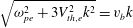 $\sqrt{\unicode[STIX]{x1D714}_{pe}^{2}+3V_{th,e}^{2}k^{2}}=v_{b}k$
, of Langmuir waves and electron beam is met initially Langmuir wave packet is generated. Subsequently, due to quasi-linear relaxation
 $v_{b}$
essentially decreases as it joins the bulk distribution therefore for the right-hand side of the latter equality to stay the same,
 $k$
needs increase. This behaviour can be clearly seen in figures 4 and 8. In the homogeneous case no electron acceleration is seen, as expected. In the case with
 $\unicode[STIX]{x0394}n=0.01$
we see appearance of negative wavenumbers
 $k$
along the expected dispersion curve (figure 6). This implies that backwards propagating Langmuir waves appear. Because parametric instabilities such as electrostatic decay (see e.g. Zakharov, Musher & Rubenchik Reference Zakharov, Musher and Rubenchik1985) are inhibited due to immobile ions, only one possibility is allowed – the appearance of negative wavenumbers
 $k$
(figures 6 and 8) can be attributed to the Langmuir wave refraction on the positive density gradient parts of the inhomogeneity. As shown by Pechhacker & Tsiklauri (Reference Pechhacker and Tsiklauri2014) for the case of Langmuir waves propagating on a single large-scale density gradient, on positive density gradient regions
 $k$
deceases, which implies that Langmuir waves are resonant with higher-velocity electrons,
 $V_{ph}=\unicode[STIX]{x1D714}_{Langmuir}/k$
, hence we see particle acceleration in the inhomogeneous case, but no acceleration in the uniform density case. Because the dispersion relation parabola is shallow, even a small increase in number density can lead to a large decrease in
 $k$
. The drift towards smaller
 $k$
, including negative
 $k$
, does not require three-wave interaction or ion-sound-mediated electrostatic decay and naturally occurs due to wave refraction alone. The negative density gradient and quasi-linear relaxation both lead to increase in
 $k$
, but do not result in the particle acceleration. For large density fluctuations with
 $\unicode[STIX]{x0394}n=0.05$
, the dispersion relation diagram (see figure 7) shows all of the features of the
 $\unicode[STIX]{x0394}n=0.01$
case, however Langmuir wave packets slide off the Langmuir dispersion parabola because of nonlinear modifications in a similar manner as described by Thurgood & Tsiklauri (Reference Thurgood and Tsiklauri2015). Note that for the time window used the resulting frequency resolution of the discrete Fourier transform is
 $\unicode[STIX]{x0394}\unicode[STIX]{x1D714}=0.0672\unicode[STIX]{x1D714}_{pe}$
, which is of the order of the separation of the power concentration from the linear dispersion relationship, with them at most being separated by a few points. As such, the significance of this separation is unclear in these figures. We find that if larger time windows are chosen (of say thousands of
 $\unicode[STIX]{x1D714}_{pe}^{-1}$
), the separation becomes clearly resolved, confirming that the feature is not just an artefact. However, such figures have too low a time resolution to show the procession to smaller-
 $k$
(the key feature) and as such are not shown here. Comparing amongst different inhomogeneous simulations, it is clear that the progression to negative-
 $k$
(i.e. the amount of Langmuir wave reflection) scales with
 $\unicode[STIX]{x0394}n$
, whereby the largest-amplitude inhomogeneous profile
 $\unicode[STIX]{x0394}n=0.05$
(viz. the profile with the steepest gradients) produces a population of backwards-propagating waves most rapidly, out-pacing less steep profiles, contrasting with the most gentle profile
 $\unicode[STIX]{x0394}n=0.01$
which reflects waves over a significantly longer time scale. This kinematic effect relating to the behaviour of Langmuir waves propagating in a longitudinally inhomogeneous medium can be observed directly in our simulations; specifically, the reflections in the density cavities are observed in the evolution of the electric field waveforms in
 $(x,t)$
-space (figures 9–11), the co-spatial mode drift to low-
 $k$
modes is observed in wavelet power spectra of the electric field (figure 12) and the concomitant acceleration of particles is seen in phase space (figure 13) – all of which will be further discussed shortly.
Time–distance diagram of electric field energy for
 $\unicode[STIX]{x0394}n=0.05$
, illustrating the temporal evolution of the spatially localised wave packets. Note the reflections of the packets between the walls of the density cavities, where the black dashed lines illustrate the density profile along
 $x$
. Levels of the colour table are logarithmically spaced, for best contrast between features (see figure 10 for corresponding quantitative information).

Embedded movie of wavelet power spectrum of the electric field in
 $(x,k)$
-space for
 $\unicode[STIX]{x0394}n=0.05$
. The localisation of wave packets on density gradients is further illustrated, as is the kinematic effect of the reduction in
 $k$
during the reflection on positive gradients (cf. figure 11). The white curve illustrates the density profile in
 $x$
, and the straight white line is the homogeneous beam–particle resonance
 $k\unicode[STIX]{x1D706}_{D}=0.072$
. Note the ‘bursty’ behaviour of the low-
 $k$
modes.

Phase-space distribution background and beam electrons. The white curve illustrates the density profile, and the red curve the localisation of electric field energy. The turning points in the density profile/concentrations of electric field energy separate distinct regions of phase space, with the production of high-velocity particle downstream of the turning points. Due to the periodic nature of the boundary, and the crossing times of the particles, these jets are quickly recycled through the boundary to the upstream regions and make multiple passes through the acceleration sites.

We also find in figures 6–8 that the
 $\unicode[STIX]{x0394}n>0$
spectra undergoes more rapid broadening towards higher positive-
 $k$
than in the
 $\unicode[STIX]{x0394}n=0$
case, and that this proceeds more rapidly for higher values of
 $\unicode[STIX]{x0394}n$
. In § 3.1, we attributed the shift to higher
 $k$
to a dynamic shift in the beam–particle resonance condition as the beam loses particles to the plateau formation. The observed rise in broadening rate as
 $\unicode[STIX]{x0394}n$
increases is thus a consequence of the enhanced deceleration of the bulk of the beam particles (i.e. more rapid plateau formation) for
 $\unicode[STIX]{x0394}n>0$
as we have previously commented on in our discussion of figures 1–3. Although the rate of the progression towards higher positive-
 $k$
is dependent on
 $\unicode[STIX]{x0394}n$
, we find that at approaching the end time the extent of the spectrum towards positive-
 $k$
is approximately the same for all runs, which is consistent with the similar end states of the
 $\unicode[STIX]{x0394}n>0$
beam’s in phase space (see figure 1).
Next, we consider the Langmuir wave behaviour in
 $(x,t)$
-space, shown in figures 9 and 10, which for the specific case of
 $\unicode[STIX]{x0394}n=0.01$
and
 $\unicode[STIX]{x0394}n=0.05$
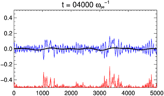
show the evolution of the electric field in
 $(x,t)$
-space in the case (blue curve), a scaled measure of electric field energy density (
 $10E_{X}^{2}-0.5$
, red curve), and the particular density profile (black curve) (i.e. they are equivalent to figure 5 for the homogeneous case). In all cases we observe an obvious localisation effect in which the wave fields and their energy densities become concentrated in the local density cavities, whereby the highest peaks often coincide with locations of maximum local gradient (corresponding to Langmuir wave turning points). This high degree of localisation leads to a clumping of energy density many orders of magnitude above background levels. We also note that this magnitude is not necessarily greater for greater
 $\unicode[STIX]{x0394}n$
, although the larger choices of
 $\unicode[STIX]{x0394}n$
result in more local density cavities with high gradients, and so we see a greater number of localised peaks, or clumps, for higher
 $\unicode[STIX]{x0394}n$
. This behaviour is completely different to the
 $\unicode[STIX]{x0394}n=0$
case shown in figure 5 (discussed in § 3.1). In the movies, one can see that the energy density localisations are propagating, although they typically remain trapped in the cavity (but they do not sit at a singular point, such as the local density minima or the local gradient maxima). In some cases, as these clumps propagate to the up the walls of a cavity, clear reflections at the local gradient maxima (which act as a turning point) can be observed (in particular, see the case of
 $\unicode[STIX]{x0394}n=0.05$
whereby many of the individual density cavities possess a steep gradient). Thus, we can directly observe the formation of a population of counter-propagating Langmuir waves due to Langmuir wave reflection off inhomogeneities which has been previously discussed in the context of the spectral results. Additionally, one can directly observe the loss of wave energy density to the high-energy particle acceleration process. As an example, consider the
 $\unicode[STIX]{x0394}n=0.01$
movie near the point
 $x=1200\unicode[STIX]{x1D706}_{D}$
from times
 $t\unicode[STIX]{x1D714}_{pe}=2000{-}4000$
. As the concentration propagates up along the cavity, it becomes trapped at the maxima and loses energy density rapidly. These reflections can also be clearly demonstrated without appealing to animation by considering time–distance diagrams of the electric field energy, as shown in figure 11 for the case
 $\unicode[STIX]{x0394}n=0.05$
. In figure 11, the reflections of waves within density cavities, associated intensification on turning points, and crossings of counter-propagating wave fronts can all be readily observed. Note, the levels chosen to produce the colour table are logarithmically spaced to enhance contrast between features (i.e. the figure provides information about the timings and location of reflections, and it is necessary to refer to figure 10 for quantitative information regarding the field amplitudes.)
The aforementioned decrease in
 $k$
seen in the Fourier spectra, which we earlier state can only be due to this refraction process, can be further confirmed by considering the evolution of wavelet power spectra of the electric fields, which allows the concentration of wave power in
 $(k,x)$
-space to be examined, i.e. unlike Fourier transforms, we can examine the distribution
 $k$
in
 $x$
. Figure 12 shows the concentration of wavelet power at instances in time for the
 $\unicode[STIX]{x0394}n=0.05$
case (specifically, the figure shows the root of wavelet power, for best contrast). The white curve illustrates the density profile in
 $x$
, and the straight white line is the homogeneous beam–particle resonance
 $k\unicode[STIX]{x1D706}_{D}=0.072$
. The black, labelled contour indicates the 95 % confidence level in the signal (see Torrence & Compo (Reference Torrence and Compo1998) for details on wavelets and their statistical properties). Crucially, the figure demonstrates that the conversion to low-
 $k$
modes occurs in the locality of the turning points – confirming our earlier description of the process (compare figure 11 with the reflections in figure 11). This qualitative behaviour is common to all inhomogeneous cases considered, and is absent in the
 $\unicode[STIX]{x0394}n=0$
case. The figure also demonstrates that some wave packets are (temporarily) converted to higher-
 $k$
modes during their propagation down negative density gradients. The movie clearly shows that the low-
 $k$
power emanates from the turning points on the density gradients, and also that the production of low-
 $k$
power occurs in a bursty fashion, which suggests that corresponding particle acceleration may also occur in bursts.
Finally, the particle acceleration concomitant to the refraction can be seen in the electron phase space, shown for the case of
 $\unicode[STIX]{x0394}n=0.05$
in figure 13. Clear qualitative differences in the beam phase space can be seen upstream and downstream of the turning points in the density gradients can be seen, with the production of high-velocity particle jets in the downstream regions. As the propagation speed of free-streaming particles is rapid compared to
 $L_{x}$
, the jets and other features cross through multiple density cavities and are rapidly recycled through the periodic boundary from the downstream region to the right to the upstream region to the left, making pinpointing particular features in phase space difficult for our specific set-up (although we stress that the periodic recycling is appropriate for our problem, which is intended to model the global properties of a beam passing through many density cavities). Further, due to disk-space restrictions and to reduce read/write operations, we only recorded the full velocity distribution (not integrated over
 $x$
) every
 $100\unicode[STIX]{x1D714}_{pe}^{-1}$
, and as such cannot directly confirm whether the bursty behaviour of the production of low-
 $k$
waves does indeed lead to a bursty particle acceleration.
These direct observations of the main physical aspects of the particle acceleration process, underpinning the changes of the beam–plasma instability in the inhomogeneous regime, are elaborated upon further in § 4.
4 Discussion
We have demonstrated in our PIC simulations that the introduction of an inhomogeneous density profile significantly affects the evolution of the electron beam–plasma instability. The variable density profile with amplitudes in excess of the threshold equation (2.4) apparently facilitates two processes that will compete to determine the overall beam energy loss and relaxation time, namely; (i) an enhanced deceleration process and thus quicker plateau formation, and (ii) an acceleration process which permits the formation of a high-energy tail.
The enhanced deceleration process occurs due to a broader range of available particle-to-wave resonances. The acceleration process is associated with the re-absorption of wave-field energy into accelerated beam particles. This process is directly facilitated due to the refraction of Langmuir waves as they propagate along a region with a positive density gradient. There is clear evidence in § 3.2 that as Langmuir waves propagate through regions of positive density gradient they experience a decrease in their wavenumber
 $k$
(see, e.g. the wavelet power spectrum, figure 12). Thus, their phase velocity
 $v_{ph}=\unicode[STIX]{x1D714}/k$
increases and so the waves exchange energy resonantly with increasingly energetic particles during their propagation up the density gradients, producing high-velocity particle jets which can be seen in phase space (figure 13). The same process has been detailed for a beam propagating on a single large-scale positive density gradient by Pechhacker & Tsiklauri (Reference Pechhacker and Tsiklauri2014).
The net effect of the two above processes was found in all inhomogeneous cases considered to be as follows; in comparison to the homogeneous case the bump in tail instability time scale is actually quicker, with a faster procession towards plateau formation, although the beam population loses much less energy overall due to the high-energy tail formation. We find no evidence of the slight positive slopes remaining in the distribution (integrated over the domain) after saturation as discussed by Voshchepynets & Krasnoselskikh (Reference Voshchepynets and Krasnoselskikh2013), rather all cases considered here appear to relax to a plateau. We also examined the local distribution functions at the end time (i.e. at specific cells in the domain) to look for evidence of localised positive slopes, however it becomes clear that the number of PPCPS leads to a somewhat noisy distribution on the slope which could well obscure slightly positive slopes. We believe it is likely that the formation of the gentle positive slopes is a subtle kinetic effect which is shown in the semi-analytical models of Voshchepynets & Krasnoselskikh (Reference Voshchepynets and Krasnoselskikh2013), but would require very high numbers of pseudoparticles to demonstrate with a PIC simulation.
We also find that all cases considered in excess of the inhomogeneity amplitude threshold tend to relax to a similar asymptotic end state, both in terms of the distribution function (figure 1) and energy distribution of particles (figure 3). This result is consistent with the work of Voshchepynets et al. (Reference Voshchepynets, Krasnoselskikh, Artemyev and Volokitin2015), who considered inhomogeneous beam–plasma interaction with a probabilistic model (see e.g. their figure 4). Our results are consistent as both studies do not venture outside a quasi-linear/weak beam regime, both are 1-D and both ignore the influence of ion-sound waves (in our case, due to ion immobilisation). At this stage, we cannot make any comments on an underlying explanation for this remarkable result, beyond noting that we have obtained the same with a PIC approach, and highlighting that the particular end state was shown to be dependent on the initial beam energy and beam density in the Voshchepynets et al. (Reference Voshchepynets, Krasnoselskikh, Artemyev and Volokitin2015) study. The end state, consisting of an asymptotic equilibrium reached between the Langmuir waves and the suprathermal electrons, has been explored in the case of kappa-distributed plasmas by Yoon (Reference Yoon2011, Reference Yoon2012a ,Reference Yoon b ). It is possible that future PIC simulations similar to those considered in this paper could provide insight into the nature of the asymptotic equilibrium, by varying parameters other than the density profile to alter the end state, and also give an indication as to whether Gaussian or Kappa distributions are more plausible equilibrium distribution functions.
In addition to the overall effect of the density cavities on the beam’s energy loss and instability saturation time it is also interesting that some individual density cavities assume steep enough gradients such that Langmuir packets are directly observed to reflect about turning points (e.g. figure 11). This shows that simple Langmuir wave kinematics in the inhomogeneous regime facilitates the development of a population of counter-propagating Langmuir waves. The presence of a population of counter-propagating Langmuir waves is an essential component in typical models of harmonic solar radio emission whereby their three-wave coalescence produces the emission. Usually, the population of counter-propagating Langmuir waves is thought to be created through electrostatic decay of the forward-propagating waves into ion-acoustic waves and backwards-propagating waves (such as in the self-consistent emission simulations of, e.g. Thurgood & Tsiklauri Reference Thurgood and Tsiklauri2015). However, in this case we find that a population of counter-propagating Langmuir waves can easily be created in the absence of such three-wave interactions, a population which could then proceed to coalesce and participate in harmonic radio emission. It should be noted that beating Langmuir waves in the absence of ion-acoustic counterparts have actually been occasionally observed in situ (e.g. Kellogg et al. Reference Kellogg, Goetz, Monson and Bale1999). It would be interesting to compare radio emission resulting from the homogeneous and inhomogeneous cases in future work, although it is likely using a full PIC approach will suffer severe computational demands (for example, the relatively expensive 1D simulations considered here would need to be extended into two dimensions to study radio emission).
As stressed in § 2, these experiments have specifically considered the influence of ‘strong’ inhomogeneity, i.e. that in excess of the fluctuation-amplitude threshold equation (2.4). We have not considered the intermediate case of inhomogeneity levels less than, or approaching, this value due to computational restrictions. Given that our PIC results broadly confirm the results of Krafft et al. (Reference Krafft, Volokitin and Krasnoselskikh2013) in the strongly inhomogeneous case, we find no reason to suggest that the physics and end state of the intermediate cases should be different to those found using their model, in which cases of weak inhomogeneity not satisfying the threshold simply proceed as per the perfectly homogeneous case.
5 Conclusions
We have for the first time shown with a fully kinetic PIC approach that plasma inhomogeneity can seriously alter behaviour of the electron beam–plasma instability, independently confirming previous theoretical predictions and modelling efforts with a clear, robust and simple numerical approach.
We find that in the case of no fluctuations (homogeneous density), the dispersion relation diagram shows that when the resonant condition,
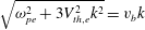 $\sqrt{\unicode[STIX]{x1D714}_{pe}^{2}+3V_{th,e}^{2}k^{2}}=v_{b}k$
, of Langmuir waves and electron beam is met, initially Langmuir wave packets are generated. Then, because of quasi-linear relaxation (when beam particles join the main population forming the plateau)
 $v_{b}$
essentially decreases as it joins the bulk distribution therefore for the right-hand side of the latter equality to stay the same, (i.e. for wave packet to stay on the dispersion curve)
 $k$
needs to increase. This behaviour can be clearly seen in figures 4 and 8. In the homogeneous case no electron acceleration is seen, as expected. In the case of
 $\unicode[STIX]{x0394}n=0.01$
, the dispersion relation (figure 6) shows appearance of negative wavenumbers. This implies that backwards propagating Langmuir waves appear. Because parametric instabilities are inhibited due to immobile ions, there is only one possibility: the appearance of negative wavenumbers (figures 6 and 8) can be attributed to the Langmuir wave refraction on the positive density gradient parts of the inhomogeneity. We have directly observed this refraction in the electric field waveforms and corresponding wavelet power spectra. As discussed by Pechhacker & Tsiklauri (Reference Pechhacker and Tsiklauri2014), at positive density gradient locations
 $k$
deceases, which means that Langmuir waves are resonant with higher-velocity electrons,
 $V_{ph}=\unicode[STIX]{x1D714}_{Langmuir}/k$
, hence we see particle acceleration in the inhomogeneous case, but no acceleration in the uniform density case. Because the dispersion relation parabola is shallow, even small increase in number density can lead to large decrease in
 $k$
(even making it negative). The key point is that drift towards smaller
 $k$
, including negative does not require three-wave interaction or ion-sound-mediated decay and naturally occurs due to wave refraction alone. (1) Negative density gradients and (2) quasi-linear relaxation both lead to increase in
 $k$
, but do not result in the particle acceleration. For the higher-level fluctuations considered, e.g.
 $\unicode[STIX]{x0394}n=0.05$
, the dispersion relation diagram (see figure 7) shows all the features of the
 $\unicode[STIX]{x0394}n=0.01$
case, however Langmuir wave packets now slide off the Langmuir dispersion parabola because of nonlinearity, in a similar manner as described by Thurgood & Tsiklauri (Reference Thurgood and Tsiklauri2015).
In conclusion, fully kinetic PIC simulations broadly confirm findings of quasi-linear and the Hamiltonian model based on Zakharov’s equations with a kinetic treatment of the beam only. We also find that the strong density fluctuations (e.g. 5 % of the background) modify properties of excited Langmuir waves altering their dispersion properties.
Acknowledgements
The authors acknowledge funding from the Leverhulme Trust Research Project grant RPG-311. The computational work for this paper was carried out on the joint BIS, STFC and SFC (SRIF) funded DiRAC-1 cluster at the University of St Andrews (Scotland, UK). The EPOCH code used in this work was in part funded by the UK EPSRC grants EP/G054950/1, EP/G056803/1, EP/G055165/1 and EP/ M022463/1. Wavelet software was provided by C. Torrence and G. Compo, and is available at URL: http://paos.colorado.edu/research/wavelets/. The authors would also like to thank the anonymous referees for their time spent reviewing the manuscript, and their constructive criticisms and input.