1 Introduction
Mixing of fluids in porous media is notoriously difficult due to the absence of inertia, and lies at the heart of many real-world problems: it plays a key role in carbon sequestration (Huppert & Neufeld Reference Huppert and Neufeld2014), oil recovery (Lake Reference Lake1989), mantle convection (van Keken, Hauri & Ballentine Reference van Keken, Hauri and Ballentine2002), microfluidic devices (Stone, Stroock & Ajdari Reference Stone, Stroock and Ajdari2004) and food processing (Hill Reference Hill1952). Ultimately mixing occurs as molecular diffusion acts to reduce local concentration gradients. It is therefore most effective when both gradients in concentration, and the surface areas across which it acts, are large. While fluids at high Reynolds numbers can be vigorously stirred by turbulence, other mechanisms are required to stir fluids in a porous medium. One such mechanism is the generation of interfacial instabilities, which increase the area over which molecular diffusion acts. Such instabilities can be driven by a number of different mechanisms including chemical reactions (Almarcha et al. Reference Almarcha, Trevelyan, Grosfils and De Wit2010), unstable density stratifications (Hewitt, Neufeld & Lister Reference Hewitt, Neufeld and Lister2013) and differences in viscosity (Tan & Homsy Reference Tan and Homsy1988). Here we focus on the effects of a planar, viscously unstable interface on mixing in porous media.
Viscous fingering is an interfacial instability that occurs when a less viscous fluid displaces a more viscous one in a porous medium or Hele-Shaw cell. This phenomenon was first described by Hill (Reference Hill1952) and later by Saffman & Taylor (Reference Saffman and Taylor1958). The instability results in a series of fine fingers whose length scale can depend on a variety of factors including surface tension and diffusion. Saffman and Taylor showed that in the case of immiscible flows (when the fluids do not mix) these fingers tend to coalesce to a single steadily propagating finger. Since the work of Saffman and Taylor, there have been a variety of studies on both the initial instability and the stability of the single-finger state (see McCloud & Maher Reference McCloud and Maher1995).
If the interfacial tension is zero, Saffman and Taylor’s theory predicts infinitesimally small fingers. However, experiments with miscible fluids in Hele-Shaw cells indicate that either the plate spacing (Paterson Reference Paterson1985; Lajeunesse et al. Reference Lajeunesse, Martin, Rakotomalala, Salin and Yortsos1999) or diffusion (Chui, De Anna & Juanes Reference Chui, De Anna and Juanes2015) between the fluids leads to finite wavelength fingers. Tan & Homsy (Reference Tan and Homsy1986) used linear stability theory, and a slowly diffusing background flow, to predict the most unstable mode and its growth. In subsequent work, they compared their theory to numerical simulations of the full two-dimensional problem (Tan & Homsy Reference Tan and Homsy1988). Since then much work has been done to understand the onset and early-time behaviour with the inclusion of a variety of stabilizing and destabilizing mechanisms such as gravity (Ruith & Meiburg Reference Ruith and Meiburg2000), Korteweg stresses (Pramanik & Mishra Reference Pramanik and Mishra2015a ,Reference Pramanik and Mishra b ) and permeability layering (De Wit & Homsy Reference De Wit and Homsy1997a ,Reference De Wit and Homsy b ).
Some recent attempts have been made to model the impact of viscous fingering on mixing beyond the onset. Jha, Cueto-Felgueroso & Juanes (Reference Jha, Cueto-Felgueroso and Juanes2011a ,Reference Jha, Cueto-Felgueroso and Juanes b ) examined the long-time mixing of a viscously unstable system containing high or low viscosity blobs in a doubly periodic domain. Informed by numerical experiments, they developed a model for the evolution of the mixing rate. Here, we instead investigate the evolution of a single viscously unstable planar interface from onset to shutdown.
Although previous work has looked at the onset problem and early-time behaviour of miscible viscous fingering, the late-time behaviour remains poorly understood. In previous work, Tan & Homsy (Reference Tan and Homsy1988) determined a critical Péclet number beyond which tip splitting occurs, and they hypothesized that this value might have implications for the asymptotic fate of the fingers. Zimmerman & Homsy (Reference Zimmerman and Homsy1992) similarly suggested that the asymptotic behaviour may include multiple steadily propagating fingers under the assumption that tip splitting may balance the upwards cascade in the scale of the fingers, but were unable to extend their numerical simulations to a final state. In experiments in a radial geometry, Chui et al. (Reference Chui, De Anna and Juanes2015) showed a transition in finger growth from a scaling with
 $t$
to one with
 $t^{1/2}$
corresponding to the shutdown of the instability. However, the ultimate fate and final form of the fingers remains unclear.
This paper has two main aims. The first aim is to identify and provide a detailed explanation of the asymptotic fate of the fingering instability. Then, given an understanding of the late-time behaviour, the second aim is to examine the full ‘life cycle’ of miscible viscous fingering from ‘onset’ to ‘shutdown’ which draws together previously disjoint or contradictory observations and claims. We find that the dynamics can be divided into three regimes: (i) at early times, the flow is well described by linear stability theory; (ii) at intermediate times, the flow is dominated by nonlinear finger interactions; and (iii) at late times, the flow is composed of an exponentially slowing, single-finger exchange flow. Ultimately, once the fingers have slowed enough, diffusion in the direction of the flow dominates the dynamics. In the course of this study, we also identify a critical Péclet number for the instability in the first regime and derive an improved averaged model for the flow in the second regime.
This paper is laid out as follows. In § 2 we formulate the problem, and we describe the numerical method used to solve this problem in § 3. In § 4 we present numerical results across a range of parameter settings and identify the dominant scalings in each regime. We then discuss the early-time linearly unstable and intermediate-time nonlinear coalescence regimes in more detail in § 5. Finally, in § 6, we discuss the late-time behaviour, for which we derive an analytic solution for the new single-finger state and compare it to the results of our numerical simulations.
2 Problem formulation
We consider a two-dimensional, isotropic porous strip of infinite extent and finite width
 $a$
(figure 1). The medium has uniform porosity
 $\unicode[STIX]{x1D719}$
and permeability
 $k$
, and is initially saturated with an ambient fluid which has viscosity
 $\unicode[STIX]{x1D707}_{2}$
. Another fluid, which is fully miscible with the ambient fluid and has viscosity
 $\unicode[STIX]{x1D707}_{1}$
, is injected at a constant velocity
 $U\hat{\boldsymbol{x}}$
. The diffusivity between the fluids is
 $D$
and gravity is neglected. Note that, in general, the permeability and diffusivity may be described by second-rank tensors, and can depend on a variety of factors including the concentration of either fluid, fluid velocity, time and space. For simplicity, the permeability and diffusion–dispersion tensors are here assumed to be isotropic and constant.
2.1 Governing equations
The two fluids are incompressible and fully miscible. The flow obeys Darcy’s law and the concentration of the injected fluid is described by an advection–diffusion equation,
 $$\begin{eqnarray}\displaystyle & \displaystyle \unicode[STIX]{x1D735}\boldsymbol{\cdot }\boldsymbol{u}=0, & \displaystyle\end{eqnarray}$$
 $$\begin{eqnarray}\displaystyle & \displaystyle \boldsymbol{u}=-\frac{k}{\unicode[STIX]{x1D707}(c)}\unicode[STIX]{x1D735}p, & \displaystyle\end{eqnarray}$$
 $$\begin{eqnarray}\displaystyle & \displaystyle \unicode[STIX]{x1D719}\frac{\unicode[STIX]{x2202}c}{\unicode[STIX]{x2202}t}+\boldsymbol{u}\boldsymbol{\cdot }\unicode[STIX]{x1D735}c=\unicode[STIX]{x1D719}D\unicode[STIX]{x1D6FB}^{2}c. & \displaystyle\end{eqnarray}$$
Here
 $\boldsymbol{u}=(u,v)$
is the Darcy velocity or fluid flux,
 $p$
the pressure and
 $c$
the concentration, which varies between 0 (in the ambient fluid) and 1 (in the injected fluid). The viscosity
 $\unicode[STIX]{x1D707}(c)$
varies with the concentration, and we follow the convention of previous authors (e.g. Tan & Homsy Reference Tan and Homsy1986; Zimmerman & Homsy Reference Zimmerman and Homsy1991; Pramanik & Mishra Reference Pramanik and Mishra2015a
) by assuming an Arrhenius-like exponential dependence,
 $$\begin{eqnarray}\displaystyle \unicode[STIX]{x1D707}(c)=\unicode[STIX]{x1D707}_{2}\text{e}^{-Rc}, & & \displaystyle\end{eqnarray}$$
where
 $R=-\text{ln}(\unicode[STIX]{x1D707}_{1}/\unicode[STIX]{x1D707}_{2})$
.
An illustration of the model set-up. The porous medium is taken to be an infinite strip of width
 $a$
initially filled with a fluid with viscosity
 $\unicode[STIX]{x1D707}_{2}$
. A fluid with viscosity
 $\unicode[STIX]{x1D707}_{1}$
is injected at a constant velocity
 $U\hat{\boldsymbol{x}}$
into the medium. We measure the concentration of the injected fluid, which is one upstream and zero downstream.

We non-dimensionalize the equations by the height of the domain
 $a$
, velocity
 $U$
, time
 $\unicode[STIX]{x1D719}a/U$
, permeability
 $k$
, viscosity of the ambient fluid
 $\unicode[STIX]{x1D707}_{2}$
and pressure
 $\unicode[STIX]{x1D707}_{2}Ua/k$
, leading to
 $$\begin{eqnarray}\displaystyle \frac{\unicode[STIX]{x2202}u^{\ast }}{\unicode[STIX]{x2202}x^{\ast }}+\frac{\unicode[STIX]{x2202}v^{\ast }}{\unicode[STIX]{x2202}y^{\ast }}=0, & & \displaystyle\end{eqnarray}$$
 $$\begin{eqnarray}\displaystyle -u^{\ast }\unicode[STIX]{x1D707}^{\ast }=\frac{\unicode[STIX]{x2202}p^{\ast }}{\unicode[STIX]{x2202}x^{\ast }},\quad -v^{\ast }\unicode[STIX]{x1D707}^{\ast }=\frac{\unicode[STIX]{x2202}p^{\ast }}{\unicode[STIX]{x2202}y^{\ast }}, & & \displaystyle\end{eqnarray}$$
 $$\begin{eqnarray}\displaystyle & \displaystyle \frac{\unicode[STIX]{x2202}c}{\unicode[STIX]{x2202}t^{\ast }}+u^{\ast }\frac{\unicode[STIX]{x2202}c}{\unicode[STIX]{x2202}x^{\ast }}+v^{\ast }\frac{\unicode[STIX]{x2202}c}{\unicode[STIX]{x2202}y^{\ast }}=\frac{1}{Pe}\left(\frac{\unicode[STIX]{x2202}^{2}c}{\unicode[STIX]{x2202}x^{\ast 2}}+\frac{\unicode[STIX]{x2202}^{2}c}{\unicode[STIX]{x2202}y^{\ast 2}}\right), & \displaystyle\end{eqnarray}$$
 $$\begin{eqnarray}\displaystyle & \displaystyle \unicode[STIX]{x1D707}^{\ast }(c)=\text{e}^{-Rc}, & \displaystyle\end{eqnarray}$$
where
 $(\cdot )^{\ast }$
denotes a dimensionless quantity. For notational simplicity, we drop the asterisks from all subsequent quantities. The key dimensionless parameters are the log-viscosity ratio and the Péclet number, defined as
 $$\begin{eqnarray}\displaystyle R=-\text{ln}\left(\frac{\unicode[STIX]{x1D707}_{1}}{\unicode[STIX]{x1D707}_{2}}\right),\quad Pe=\frac{Ua}{\unicode[STIX]{x1D719}D}. & & \displaystyle\end{eqnarray}$$
When the injected fluid is more viscous than the ambient (
 $R<0$
), the interface is stable and the concentration evolves by diffusion alone, with a classical error-function profile. However, when the injected fluid is less viscous than the ambient (
 $R>0$
), the interface can be unstable, leading to complex fingering patterns. We focus on the latter problem here. The Péclet number provides a ratio of the characteristic time scales for diffusion and advection: when
 $Pe\ll 1$
, diffusion dominates the dynamics, and when
 $Pe\gg 1$
, advection dominates. In the diffusive limit, as will be shown later, the instability can be suppressed so we will, therefore, focus predominantly on the limit
 $Pe\gg 1$
.
We note that the Péclet number here is a macroscopic quantity defined with respect to the width
 $a$
of the porous medium. It is distinct from the pore Péclet number,
 $Pe_{p}=Ub/D=(b/a)Pe$
, which is defined with respect to the intrinsic length scale
 $b$
of the medium, i.e. the pore size, or, in a Hele-Shaw cell, the gap width. The assumption of Darcy flow relies on the pore Péclet number being small,
 $Pe_{p}<O(1)$
(Yang & Yortsos Reference Yang and Yortsos1997), or, equivalently,
 $a/b>O(Pe)$
. In this limit, diffusion acts quickly to homogenize flow structures at the pore scale. This limit is assumed in all the work presented in this paper. If, instead,
 $Pe_{p}$
were not small, the flow structures across the pore or gap width would affect the global dynamics, leading to qualitatively different macroscopic behaviour (Paterson Reference Paterson1985; Lajeunesse et al.
Reference Lajeunesse, Martin, Rakotomalala, Salin and Yortsos1999).
We work in a reference frame moving with the velocity of the injected fluid, and introduce transformed variables
 $$\begin{eqnarray}\displaystyle \tilde{u} =u-1,\quad \tilde{x}=x-t. & & \displaystyle\end{eqnarray}$$
In this frame, equations (2.5)–(2.7) become
 $$\begin{eqnarray}\displaystyle \frac{\unicode[STIX]{x2202}\tilde{u} }{\unicode[STIX]{x2202}\tilde{x}}+\frac{\unicode[STIX]{x2202}v}{\unicode[STIX]{x2202}y}=0, & & \displaystyle\end{eqnarray}$$
 $$\begin{eqnarray}\displaystyle -(\tilde{u} +1)\unicode[STIX]{x1D707}=\frac{\unicode[STIX]{x2202}p}{\unicode[STIX]{x2202}\tilde{x}},\quad -v\unicode[STIX]{x1D707}=\frac{\unicode[STIX]{x2202}p}{\unicode[STIX]{x2202}y}, & & \displaystyle\end{eqnarray}$$
 $$\begin{eqnarray}\displaystyle \frac{\unicode[STIX]{x2202}c}{\unicode[STIX]{x2202}t}+\tilde{u} \frac{\unicode[STIX]{x2202}c}{\unicode[STIX]{x2202}\tilde{x}}+v\frac{\unicode[STIX]{x2202}c}{\unicode[STIX]{x2202}y}=\frac{1}{Pe}\left(\frac{\unicode[STIX]{x2202}^{2}c}{\unicode[STIX]{x2202}\tilde{x}^{2}}+\frac{\unicode[STIX]{x2202}^{2}c}{\unicode[STIX]{x2202}y^{2}}\right). & & \displaystyle\end{eqnarray}$$
Again, for notational convenience, we drop the tildes from all subsequent quantities.
2.2 Boundary conditions
Similar to previous work (Tan & Homsy Reference Tan and Homsy1988), we impose periodicity at the top and bottom boundaries. The upstream and downstream concentration are fixed at
 $c=1$
and
 $c=0$
respectively and the horizontal velocity is fixed at
 $u=0$
(in the moving frame). The boundary conditions are thus
 $$\begin{eqnarray}\displaystyle c(x,0,t)=c(x,1,t),\quad u(x,0,t)=u(x,1,t),\quad v(x,0,t)=v(x,1,t), & & \displaystyle\end{eqnarray}$$
 $$\begin{eqnarray}\displaystyle c(-\infty ,y,t)=1,\quad c(\infty ,y,t)=0, & & \displaystyle\end{eqnarray}$$
 $$\begin{eqnarray}\displaystyle u(-\infty ,y,t)=u(\infty ,y,t)=0. & & \displaystyle\end{eqnarray}$$
2.3 Diagnostic quantities
As the instability develops and an array of fine fingers form, the local fingering dynamics become chaotic and are controlled by nonlinear interactions between fingers. Instead of examining the behaviour of each individual finger, we aim to examine how the fingering dynamics evolve globally. To do so, we compute the average concentration over the transverse direction,
 $$\begin{eqnarray}\displaystyle \overline{c}(x,t)=\int _{0}^{1}c(x,y,t)\,\text{d}y. & & \displaystyle\end{eqnarray}$$
Using this definition, and defining the deviations
 $c^{\prime }(x,y)=c(x,y)-\overline{c}(x)$
, equation (2.13) can be written as two coupled equations for the mean and perturbed concentrations,
 $$\begin{eqnarray}\displaystyle & \displaystyle \frac{\unicode[STIX]{x2202}\overline{c}}{\unicode[STIX]{x2202}t}+\frac{\unicode[STIX]{x2202}\overline{uc^{\prime }}}{\unicode[STIX]{x2202}x}=\frac{1}{Pe}\frac{\unicode[STIX]{x2202}^{2}\overline{c}}{\unicode[STIX]{x2202}x^{2}}, & \displaystyle\end{eqnarray}$$
 $$\begin{eqnarray}\displaystyle & \displaystyle \frac{\unicode[STIX]{x2202}c^{\prime }}{\unicode[STIX]{x2202}t}+\frac{\unicode[STIX]{x2202}uc^{\prime }}{\unicode[STIX]{x2202}x}+\frac{\unicode[STIX]{x2202}u\overline{c}}{\unicode[STIX]{x2202}x}-\frac{\unicode[STIX]{x2202}\overline{uc^{\prime }}}{\unicode[STIX]{x2202}x}+\frac{\unicode[STIX]{x2202}vc^{\prime }}{\unicode[STIX]{x2202}y}=\frac{1}{Pe}\left(\frac{\unicode[STIX]{x2202}^{2}c^{\prime }}{\unicode[STIX]{x2202}x^{2}}+\frac{\unicode[STIX]{x2202}^{2}c^{\prime }}{\unicode[STIX]{x2202}y^{2}}\right). & \displaystyle\end{eqnarray}$$
We will use this decomposition in our derivation of the late-time solution in § 6.
We also examine three global quantities over time: the mixing length
 $h$
, which quantifies the width of the mixing zone; the average number of fingers
 $n$
, which gives an inverse measure of the transverse length scale; and the Nusselt number,
 $Nu$
, which quantifies the total convective mixing rate. These quantities are defined as
 $$\begin{eqnarray}\displaystyle & \displaystyle h=x|_{\overline{c}=0.01}-x|_{\overline{c}=0.99}, & \displaystyle\end{eqnarray}$$
 $$\begin{eqnarray}\displaystyle & \displaystyle n=\frac{1}{h}\int _{x|_{\overline{c}=0.99}}^{x|_{\overline{c}=0.01}}\unicode[STIX]{x1D702}(x)\,\text{d}x, & \displaystyle\end{eqnarray}$$
 $$\begin{eqnarray}\displaystyle & \displaystyle Nu=\int _{-\infty }^{\infty }\int _{0}^{1}u\left(c-\frac{1}{2}\right)\,\text{d}y\,\text{d}x, & \displaystyle\end{eqnarray}$$
where the number of fingers
 $\unicode[STIX]{x1D702}(x)$
is calculated by counting the number of local maxima in a vertical slice. Note that the Nusselt number is often defined as
 $Nu^{\ast }=1+Pe\,Nu$
, which is the ratio between total transport and diffusive transport (Zhou Reference Zhou2013). Here we instead use the Nusselt number simply to quantify the convective transport.
3 Numerical method
A variety of techniques have been used to solve the coupled equations (2.8), (2.11)–(2.13) including spectral (Tan & Homsy Reference Tan and Homsy1988; Zimmerman & Homsy Reference Zimmerman and Homsy1991, Reference Zimmerman and Homsy1992; De Wit & Homsy Reference De Wit and Homsy1997b
), pseudo-spectral (Islam & Azaiez Reference Islam and Azaiez2005) and finite-difference methods (Jha et al.
Reference Jha, Cueto-Felgueroso and Juanes2011a
,Reference Jha, Cueto-Felgueroso and Juanes
b
). Here we use a modified finite-difference method, which is numerically stable for all
 $R$
.
Given that the fluids are incompressible, we write the velocity in terms of a streamfunction
 $\unicode[STIX]{x1D6F9}(x,y,t)$
,
 $$\begin{eqnarray}\displaystyle u=\frac{\unicode[STIX]{x2202}\unicode[STIX]{x1D6F9}}{\unicode[STIX]{x2202}y},\quad v=-\frac{\unicode[STIX]{x2202}\unicode[STIX]{x1D6F9}}{\unicode[STIX]{x2202}x}. & & \displaystyle\end{eqnarray}$$
Eliminating the pressure from (2.12) and combining with (3.1) and (2.8) results in a nonlinear elliptic equation for the streamfunction,
 $$\begin{eqnarray}\displaystyle \frac{\unicode[STIX]{x2202}^{2}\unicode[STIX]{x1D6F9}}{\unicode[STIX]{x2202}x^{2}}+\frac{\unicode[STIX]{x2202}^{2}\unicode[STIX]{x1D6F9}}{\unicode[STIX]{x2202}y^{2}}-R\frac{\unicode[STIX]{x2202}c}{\unicode[STIX]{x2202}x}\frac{\unicode[STIX]{x2202}\unicode[STIX]{x1D6F9}}{\unicode[STIX]{x2202}x}-R\frac{\unicode[STIX]{x2202}c}{\unicode[STIX]{x2202}y}\frac{\unicode[STIX]{x2202}\unicode[STIX]{x1D6F9}}{\unicode[STIX]{x2202}y}=R\frac{\unicode[STIX]{x2202}c}{\unicode[STIX]{x2202}y}, & & \displaystyle\end{eqnarray}$$
with boundary conditions
 $$\begin{eqnarray}\displaystyle & \displaystyle \unicode[STIX]{x1D6F9}(x,0,t)=\unicode[STIX]{x1D6F9}(x,1,t), & \displaystyle\end{eqnarray}$$
 $$\begin{eqnarray}\displaystyle & \displaystyle \unicode[STIX]{x1D6F9}(-\infty ,y,t)=\unicode[STIX]{x1D6F9}(\infty ,y,t)=0, & \displaystyle\end{eqnarray}$$
In order to simulate an infinite strip, we impose boundary conditions (2.15) and (3.4) at
 $x=\pm \unicode[STIX]{x1D6E4}/2$
, where
 $\unicode[STIX]{x1D6E4}$
is chosen to be sufficiently large such that these boundaries are far from the fingered region. Furthermore, since previous work has shown that solutions are independent of the aspect ratio as long as the fingered region is sufficiently far from the boundaries (Tan & Homsy Reference Tan and Homsy1988; Ruith & Meiburg Reference Ruith and Meiburg2000), we use a growing domain to minimize computational time. Each simulation is initialized with a domain length
 $\unicode[STIX]{x1D6E4}=1$
, and
 $\unicode[STIX]{x1D6E4}$
is doubled whenever
 $\overline{c}(x=-0.3\unicode[STIX]{x1D6E4})=0.999$
or
 $\overline{c}(x=0.3\unicode[STIX]{x1D6E4})=0.001$
. We compared simulations with variable and fixed domain sizes to confirm that this mapping had no measurable effect on the dynamics.
We discretize the domain on a rectangular grid with
 $(n_{x},n_{y})$
grid points in the
 $(x,y)$
direction. Each simulation is initialized with an almost sharp interface and an added small random perturbation centred at
 $x=0$
,
 $$\begin{eqnarray}\displaystyle c_{0}=\frac{1}{2}+\frac{1}{2}\text{erf}\left(-\frac{x}{\sqrt{t_{0}}}\right)+r(x,y)\text{e}^{-x^{2}/t_{0}}, & & \displaystyle\end{eqnarray}$$
where the function
 $r(x,y)$
returns a uniformly distributed random number on the interval
 $[0,10^{-5}]$
. The diffusive error function with small effective time origin
 $t_{0}$
is included in (3.5) to aid the accuracy of the numerical scheme at early times. We set
 $t_{0}=10^{-6}$
in all simulations.
At each time step, we solve (3.2) using an iterative multi-grid solver (Adams Reference Adams1999) with the solution at the previous time step used as an initial guess. We use sixth-order compact finite differences (Lele Reference Lele1992) to discretize the spatial derivatives in (3.2) and (2.13) and advance (2.13) in time using a third-order Runge–Kutta scheme. We select the time step,
 $\unicode[STIX]{x1D6FF}t=\text{min}(10^{-3},\text{min}(\unicode[STIX]{x1D6FF}x/u_{max},\unicode[STIX]{x1D6FF}y/v_{max}))$
, to always satisfy the Courant–Friedrichs–Lewy condition. To validate the numerical method, we tested the convergence of the solution with increased spatial and temporal resolution and compared the growth rate of single-mode perturbations to the linear stability theory of Tan & Homsy (Reference Tan and Homsy1986).
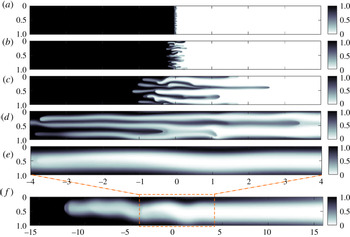
Colour maps of the concentration field (in a frame moving with the interface) over the course of a simulation. Here,
 $R=2$
and
 $Pe=2000$
. Snapshots, from top to bottom, are taken at (a)
 $t=0.5$
, (b)
 $t=1$
, (c)
 $t=3$
, (d)
 $t=10$
, (e,f)
 $t=31$
. Note that the numerical domain is significantly larger than shown in the lower three panels. Panel (f) is zoomed out to include the full finger and note that the figure is horizontally compressed by a factor of 4.

4 Fingering pattern and regimes
Figure 2 shows a sequence of snapshots from a typical simulation for log-viscosity ratio
 $R=2$
and Péclet number
 $Pe=2000$
. At early times, the initially very sharp interface begins to smooth out and a series of fine fingers develop (figure 2
a). At intermediate times, once the fingers reach a certain amplitude, they begin to interact, which drives coarsening in the vertical direction and growth in the horizontal direction (figure 2
b–d). Overall, these nonlinear interactions lead to coalescence until a single broad finger remains (figure 2
e,f).
All of our numerical simulations, which have
 $Pe$
ranging from
 $100$
to
 $16\,000$
and
 $R$
ranging from
 $1$
to
 $5$
, show this qualitative behaviour. In general, we find that at early times the interface diffuses and a set of fingers develop. The number of fingers that develop increases with both the Péclet number and the log-viscosity ratio. The fingers then interact nonlinearly via a variety of different mechanisms. These include shielding, when a longer finger widens at the tip and shields the growth of smaller neighbouring fingers; fading, when a finger stops growing and diffuses into the ambient; and coalescence, when two or more fingers merge together. When the Péclet number and log-viscosity ratio are large, the fingers also exhibit more complex behaviour including tip splitting, when a finger splits into two at the tip; and branching, when a finger sheds fingers from its side (Tan & Homsy Reference Tan and Homsy1988; Zimmerman & Homsy Reference Zimmerman and Homsy1991; Islam & Azaiez Reference Islam and Azaiez2005).
Regardless of the Péclet number and log-viscosity ratio, these interactions, on aggregate, lead to coalescence until a single broad finger remains. This finding is contrary to previous suggestions that the final state may include multiple fingers (Tan & Homsy Reference Tan and Homsy1988; Zimmerman & Homsy Reference Zimmerman and Homsy1992). The single finger that remains diffuses while propagating at an exponentially slowing speed, ultimately leaving a linear background concentration gradient that is gradually smoothed out by diffusion. We find that the final mixing zone length increases with both
 $R$
and
 $Pe$
.
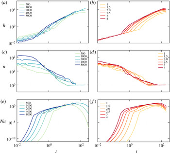
(a,b) The mixing length
 $h$
, (c,d) the number of fingers
 $n$
and (e,f) the Nusselt number
 $Nu$
plotted as functions of time. To reduce the noise in the data, two different simulations are averaged. (a,c,e) Data for log-viscosity ratio
 $R=2$
and different Péclet numbers
 $Pe$
are as marked. The black circles correspond to the snapshots in figure 2. (b,d,f) Data for
 $Pe=1000$
and different values of
 $R$
are as marked.

Figure 3 shows the mixing length
 $h$
, number of fingers
 $n$
and Nusselt number
 $Nu$
as functions of time for different Péclet numbers (a,c,e) and log-viscosity ratios (b,d,f). Figure 3(a,b) shows that the mixing length initially grows, then steepens, before finally slowing towards a constant. The early-time mixing length is larger for small Péclet numbers and is independent of the log-viscosity ratio whereas the final mixing length increases with both the Péclet number and log-viscosity ratio. Figure 3(c,d) shows the average number of fingers is fairly constant at early times, decays to one at intermediate times and stays constant at one at late times. Although the initial number of fingers increases with the Péclet number and log-viscosity ratio, the flow always tends to a single finger eventually, irrespective of the parameters. Finally, figure 3(e,f) shows that the Nusselt number first grows exponentially, then grows more slowly and finally decays exponentially.
Based on these sets of observations we partition the flow into three distinct regimes: (i) an early-time, linearly unstable regime: the mixing zone grows diffusively and fingers grow exponentially; (ii) an intermediate-time nonlinear regime: fingers coalesce and the mixing length and Nusselt number exhibit power-law growth; and (iii) a late-time, single-finger exchange-flow regime: a single pair of counter-propagating fingers slow exponentially.
Each regime shows different dynamics and exhibits different scalings. We explore these scalings in the following subsection, before examining each regime in more detail in §§ 5 and 6.
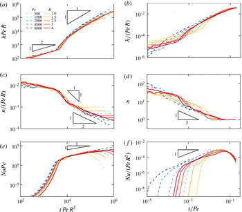
Rescaled plots of (a,b)
 $h$
, (c,d)
 $n$
and (e,f)
 $Nu$
for early times (a,c,e) and late times (b,d,f). The dashed lines are for constant
 $R=2$
and different
 $Pe$
as marked, while the solid lines are for constant
 $Pe=1000$
and different
 $R$
as marked. To reduce the noise in the data, two different simulations are averaged.

4.1 Scalings
At the start of all simulations, the interface is relatively sharp and the concentration and velocity perturbations are small. Diffusion across the interface dominates the growth of the mixing zone, and a diffusive balance
 $c/t\sim c/Peh^{2}$
gives the scaling for the mixing length
 $h\sim (t/Pe)^{1/2}$
, as can be seen in figure 4(a). In this linearly unstable regime, the aspect ratio of the fingers is
 $O(1)$
; hence, from incompressibility,
 $u/x\sim v/y\Rightarrow u\sim v$
. The linearized elliptic equation (3.2) further suggests a balance
 $u/y\sim v/x\sim Rc/y$
, or
 $u\sim v\sim R$
. The linear scaling of the velocity with the log-viscosity ratio, together with an advection–diffusion balance in (2.13), indicates that
 $c/t\sim uc/x\sim c/Pex^{2}$
, or
 $t\sim 1/R^{2}Pe$
and
 $x\sim 1/RPe$
. That is, at early times, the number of fingers scales linearly with both
 $R$
and
 $Pe$
. Figure 4(c) shows a rescaled plot of the number of fingers which collapses well with this scaling. Finally, the Nusselt number is defined as the product of the exponentially growing velocity
 $u\sim R\text{e}^{\unicode[STIX]{x1D70E}t}$
and concentration perturbations
 $c^{\prime }\sim \text{e}^{\unicode[STIX]{x1D70E}t}$
integrated over the size of the perturbations
 $x\sim 1/RPe$
(where
 $\unicode[STIX]{x1D70E}$
is the growth rate of the instability). Given the time scale identified above,
 $t\sim 1/R^{2}Pe$
, we collapse the data for the Nusselt number with the scaling
 $Nu\sim \text{e}^{tR^{2}Pe}/Pe$
(figure 4
e).
At intermediate times the fingers interact nonlinearly causing them to elongate and coarsen. The horizontal velocity remains relatively constant and is solely a function of the log-viscosity ratio,
 $u=U(R)$
. An advective balance in (2.13) gives the scaling
 $Uc/h\sim c/t$
, or
 $h\sim U(R)t$
, and this linear growth of the mixing zone in time can be seen in figure 4(a,b). In fact, we return to the functional form of the velocity
 $U(R)$
in § 5.2, and find that it can be approximated by
 $U\sim R$
for small
 $R$
. The number of fingers,
 $n$
, in the intermediate regime, follows two distinct coalescence regimes. Initially the coalescence is advectively dominated, and in this limit (2.13) gives the scaling
 $vc/(1/n)\sim c/t$
. Assuming that the transverse velocity is
 $O(R)$
and constant, then
 $n\sim 1/Rt$
. Subsequently, the flow becomes diffusively dominated and (2.13) gives the scaling
 $c/t\sim c/(Pe/n^{2})\Rightarrow n\sim (t/Pe)^{-1/2}$
. These two scaling laws can be seen in figure 4(c,d). In the intermediate-time regime, the Nusselt number scales with the width of the mixing region (
 $h\sim Rt$
) and the average convective flux, which scales with the velocity
 $U\sim R$
. Together, this gives the scaling
 $Nu\sim R^{2}t$
(see figure 4
e,f). These observations suggest that the Nusselt number and growth of the mixing zone are independent of the Péclet number and, after a small amount of time spent advectively coalescing, the finger coalescence becomes independent of the viscosity ratio.
Finally, at late times, a single pair of long, thin fingers counter-propagate and decay through a background concentration gradient. As seen in figure 4(d), all simulations tend to this single-pair (single-maxima) state. Assuming that the concentration deviations from the background are small and applying a long, thin approximation to equation (3.2) results in the scaling
 $u\sim R$
(as discussed in more detail in § 6). Balancing longitudinal advection and transverse diffusion over a single finger yields the scaling
 $Rc/h\sim 1/Pe\Rightarrow h\sim RPe$
. This tendency towards a constant mixing length proportional to
 $RPe$
is shown in figure 4(b). A diffusive balance,
 $c/t\sim 1/Pe$
, suggests that the time should be scaled by the Péclet number in this late-time regime. Applying the same argument as before, the Nusselt number decays exponentially like
 $Nu\sim PeR^{2}\text{e}^{-t/Pe}$
.
The transitions between these different regimes are controlled by the relevant time scalings in each regime. The transition from the early-time to intermediate-time regime occurs once the concentration perturbations saturate and the flow becomes nonlinear. Since the perturbations grow exponentially, and the time scale of their growth is
 $t\sim 1/R^{2}Pe$
, the perturbations will reach a certain amplitude at a time,
 $t\sim O(1/R^{2}Pe)$
. The transition to the late-time regime occurs once the flow coarsens to a single finger. Since this coarsening process is diffusively dominated, the fingers will coarsen to one finger once the flow has diffused over the entire transverse length. This means the transition between the intermediate-time and late-time regime occurs at
 $t\sim O(Pe)$
.
The scalings are summarized in table 1. In the following sections, we discuss each of these regimes in more detail with an emphasis placed on understanding the evolution of the transversely averaged concentration.
5 Early-time and intermediate-time regimes
5.1 Early times: linearly unstable regime
The concentration gradient between the two fluids, which are not moving relative to each other, is initially very high and spreads by diffusion. Neglecting the very small initial perturbations in (3.5), the resultant concentration profile is one-dimensional and given by
 $$\begin{eqnarray}\displaystyle c(x,t)=\frac{1}{2}+\frac{1}{2}\text{erf}\left(-\frac{x}{\sqrt{4t/Pe}}\right). & & \displaystyle\end{eqnarray}$$
Therefore, before the instability manifests itself, the concentration front widens like
 $(t/Pe)^{1/2}$
, which corresponds to the early-time scaling of
 $h$
(see figure 4
a).
(a)
 $Nu(t)$
, attained from direct numerical simulations, plotted on logarithmic axes for
 $R=2$
and different
 $Pe$
as marked. The Nusselt number is strictly decreasing for
 $Pe=20$
, but has a period of growth for
 $Pe=30$
, suggesting a point of marginal stability between
 $Pe=20$
and
 $30$
. (b,c) Marginal stability curves (
 $\unicode[STIX]{x1D70E}=0$
, outlines) and regions of instability (
 $\unicode[STIX]{x1D70E}>0$
, shaded areas), for
 $R=3$
and (b)
 $Pe=25,200,500$
and (c)
 $Pe=15,20,25$
. Wavenumbers less than
 $k=2\unicode[STIX]{x03C0}$
cannot be contained within the domain, and so the flow is stable for
 $k<2\unicode[STIX]{x03C0}$
, as indicated by the grey region in (c). (d) Plot of the critical Péclet number versus log-viscosity ratio based on the linear stability analysis (black line) and numerical simulations (blue ranges). The lower and upper estimated values of
 $Pe_{c}$
from our simulations in (d) are given, respectively, by the largest Pe for which
 $Nu(t)$
monotonically decreases, and by the smallest
 $Pe$
for which
 $Nu(t)$
increases at any time.

Scalings for
 $h$
,
 $n$
and
 $Nu$
for early, intermediate and late times. The transition from the early-time to intermediate-time regime occurs at
 $t\sim O(1/R^{2}Pe)$
and the transition from the intermediate-time to late-time regime occurs at
 $t\sim O(Pe)$
.

When
 $R>0$
, the flow rapidly develops a viscous-fingering instability in which perturbations grow exponentially. Many authors have explored the onset of viscous fingering in a variety of contexts using linear stability theory. Tan & Homsy (Reference Tan and Homsy1987) found that the instability can be suppressed for all times, in a radial geometry, if the Péclet number is below some critical value. In a planar geometry, however, Pramanik & Mishra (Reference Pramanik and Mishra2015a
) found a time-dependent critical Péclet number which decreases in time, and suggested that there may be no Péclet number for which the flow is always stable.
In this section, we show that there is, in fact, a critical Péclet number below which the flow is always stable in a bounded planar geometry. To motivate the existence of this critical Péclet number, figure 5(a) shows
 $Nu(t)$
for
 $R=2$
and small Péclet numbers. For the range of Péclet numbers plotted, the Nusselt number never transitions to power-law growth, suggesting that there are choices of parameters where the flow never enters the nonlinear regime. In fact, we notice that for Péclet numbers less than or equal to 20, the Nusselt number is strictly decreasing, implying the configuration is stable for all times, while for Péclet numbers greater than or equal to 30, the Nusselt number goes through a period of growth. In this section, we perform a linear stability analysis to show the existence of a critical Péclet number for the instability.
We start with a diffusive base-state solution of the unperturbed system
 $c_{0}(x,t)$
given by (5.1). To accommodate the rapidly varying base state at early times we use a similarity transformation
 $\unicode[STIX]{x1D709}=x/\sqrt{t}$
, in terms of which (5.1) is steady,
 $$\begin{eqnarray}\displaystyle c_{0}(\unicode[STIX]{x1D709})=\frac{1}{2}\left[1+\text{erf}\left(\frac{-\unicode[STIX]{x1D709}\sqrt{Pe}}{2}\right)\right]. & & \displaystyle\end{eqnarray}$$
We then linearize equations (2.13), (3.1), and (3.2) about this base state and look for perturbations of the form
 $u^{\prime }(\unicode[STIX]{x1D709},y,t)=\unicode[STIX]{x1D719}(\unicode[STIX]{x1D709})\unicode[STIX]{x1D70F}(t)\text{e}^{\text{i}ky}$
and
 $c^{\prime }(\unicode[STIX]{x1D709},y,t)=\unicode[STIX]{x1D6FD}(\unicode[STIX]{x1D709})\unicode[STIX]{x1D70F}(t)\text{e}^{\text{i}ky}$
, which satisfy
 $$\begin{eqnarray}\displaystyle & \displaystyle \left(\unicode[STIX]{x1D70E}(t_{0})-\frac{\unicode[STIX]{x1D709}}{2t_{0}}\frac{\text{d}}{\text{d}\unicode[STIX]{x1D709}}-\frac{1}{Pe\,t_{0}}\frac{\text{d}^{2}}{\text{d}\unicode[STIX]{x1D709}^{2}}+\frac{k^{2}}{Pe}\right)\unicode[STIX]{x1D6FD}=-\frac{1}{\sqrt{t_{0}}}\frac{\text{d}c_{0}}{\text{d}\unicode[STIX]{x1D709}}\unicode[STIX]{x1D719}, & \displaystyle\end{eqnarray}$$
 $$\begin{eqnarray}\displaystyle & \displaystyle \left(\frac{1}{t_{0}}\frac{\text{d}^{2}}{\text{d}\unicode[STIX]{x1D709}^{2}}-\frac{R}{t_{0}}\frac{\text{d}c_{0}}{\text{d}\unicode[STIX]{x1D709}}\frac{\text{d}}{\text{d}\unicode[STIX]{x1D709}}-k^{2}\right)\unicode[STIX]{x1D719}=-Rk^{2}\unicode[STIX]{x1D6FD}, & \displaystyle\end{eqnarray}$$
where
 $\unicode[STIX]{x1D70E}(t_{0})\equiv (1/\unicode[STIX]{x1D70F})(\text{d}\unicode[STIX]{x1D70F}/\text{d}t)|_{t=t_{0}}$
is the instantaneous growth rate at
 $t=t_{0}$
, such that
 $\unicode[STIX]{x1D70F}=\text{e}^{\int _{0}^{t}\unicode[STIX]{x1D70E}\,\text{d}t_{0}}$
(see also Pramanik & Mishra Reference Pramanik and Mishra2015a
). We note that this formulation does not require any assumption of a slowly varying or quasi-steady background. We solve (5.3) and (5.4) by discretizing the domain using standard second-order finite-difference approximations for the differential operators, which yields the matrix eigenvalue problem
 $$\begin{eqnarray}\displaystyle \unicode[STIX]{x1D648}\unicode[STIX]{x1D6FD}=\unicode[STIX]{x1D70E}\unicode[STIX]{x1D6FD}. & & \displaystyle\end{eqnarray}$$
The growth rate of the most unstable mode is given by the maximum eigenvalue of the matrix
 $\unicode[STIX]{x1D648}$
. This growth rate depends on
 $Pe$
and
 $R$
, as well as, time
 $t_{0}$
and the wavenumber of the perturbation
 $k$
.
Figure 5(b) shows the marginal stability curve
 $\unicode[STIX]{x1D70E}(k,t_{0})=0$
, where
 $\unicode[STIX]{x1D70E}$
is the growth rate of the most unstable mode, for
 $R=3$
and a variety of Péclet numbers. The system is always initially stable and goes unstable at a critical time
 $t_{0}^{\ast }>0$
. Zooming into the region around wavenumber
 $k=2\unicode[STIX]{x03C0}$
(figure 5
c), which is the largest mode that is permissible inside the domain, we notice that for
 $Pe=20$
, the marginal stability curve lies above
 $k=2\unicode[STIX]{x03C0}$
for only a finite amount of time: once the marginal stability curve falls below this value, the flow is again stable. In fact, this transition back to stability at large
 $t_{0}$
is a general feature for all
 $R$
and
 $Pe$
and this intermittent stability suggests that if the interface is diffuse enough, the instability can be suppressed, in agreement with experimental evidence (Loggia et al.
Reference Loggia, Rakotomalala, Salin and Yortsos1998). Finally, we notice that for Péclet numbers smaller than some critical value
 $Pe_{c}(R)$
, the growth rate is only positive for wavenumbers smaller than
 $2\unicode[STIX]{x03C0}$
. These modes do not fit in the domain and the interface is therefore always stable. For example, in figure 5(c) the critical Péclet number lies between 15 and 20.
The transitions out of, and back into, stability, occur as diffusion tends to arrest the instability. The system is initially stable because, for small
 $t$
, the growth of the interface (
 $O(t^{-1/2})$
) outpaces the exponential growth of the perturbations. Matching the diffusive length scale (
 $t^{1/2}/Pe^{1/2}$
) to the length scale of the most unstable perturbation (
 $1/RPe$
) gives a transition time
 $t\sim 1/R^{2}Pe$
. At sufficiently large times, the base flow is again stable, because the background concentration gradient has weakened to such an extent that transverse diffusion (
 $1/Pey^{2}$
) can smear out the advective growth of perturbations (
 $u(\unicode[STIX]{x2202}\overline{c}/\unicode[STIX]{x2202}x)\sim R(Pe^{1/2}/t^{1/2})$
). Balancing these two terms for
 $y\sim O(1)$
gives a transition time to return to stability,
 $t\sim R^{2}Pe^{3}$
. At some critical Péclet number,
 $Pe_{c}$
, the time scales of the initial instability and subsequent stabilization match, and the instability is completely suppressed. This balance gives
 $Pe_{c}\sim 1/R$
. The transition back to stability also indicates that fingering can be prevented by allowing the interface to diffuse before injection for a time
 $O(R^{2}Pe^{3})$
, or by initializing (for example by pre-mixing) a concentration gradient of width
 $O(RPe)$
.
Figure 5(d) shows
 $Pe_{c}(R)$
calculated from the linear stability analysis, which agrees with this predicted scaling. The figure also shows estimates of
 $Pe_{c}$
from direct numerical simulations, which give a reasonable agreement with the theory.
5.2 Intermediate times: nonlinear coalescence regime
The linear instability results in a number of fingers which grow exponentially and independently of their neighbours. After some time, the fingers begin to interact with each other. Although the nonlinear finger interactions exhibit complex and chaotic patterns and vary significantly over time and from simulation to simulation, the number of fingers, mixing length and Nusselt number are largely indifferent to the exact intermediary mechanisms (see rescaled data in figure 4). The transversely averaged concentration is asymmetric, nonlinear and evolves in a self-similar fashion (figure 6 a). There have been many attempts to model the behaviour of the transversely averaged concentration, with one of the simplest and most widely used models being the empirically derived formula of Koval (Reference Koval1963). While this model has been revisited by multiple authors (Yortsos & Salin Reference Yortsos and Salin2006; Booth Reference Booth2010), a fully closed model is yet to be derived. In this section we start by re-deriving the simple model that was first proposed by Koval (hereafter, the ‘simple Koval model’), and comment on its strengths and shortcomings. In order to address one of these shortcomings, we then propose a simple improvement to the model, which gives a qualitative improvement when compared with the numerical simulations.
(a) Plot of the transversely averaged concentration against the similarity variable
 $x/t$
. Here
 $R=2$
,
 $Pe=1000$
and the time, given by the colour, ranges from
 $10$
to
 $20$
. Each curve plotted represents the average of five different simulations. The dashed lines represent the three different model solutions: simple Koval (blue, dashed), fitted Koval (green, dotted) and parabolic Koval (black, dot-dashed). (b) Plot of the transverse variance in concentration for
 $Pe=2000$
,
 $4000$
,
 $8000$
and
 $16\,000$
at
 $t=8,4,2$
and
 $1$
. By sampling at these different times, we normalize for the effect of the onset of the instability. The variance calculated from the simple Koval model is given by the blue dashed line.

The simple Koval model can be derived in the limit where both the aspect ratio of the fingers and the Péclet number are large, (
 $hn\gg 1$
and
 $Pe\gg 1$
respectively). Under these conditions the flow is predominantly horizontal and longitudinal diffusion is negligible. The velocity is calculated by taking the leading-order expansion in
 $hn$
in (3.2),
 $$\begin{eqnarray}\displaystyle \frac{\unicode[STIX]{x2202}u}{\unicode[STIX]{x2202}y}-Ru\frac{\unicode[STIX]{x2202}c}{\unicode[STIX]{x2202}y}=R\frac{\unicode[STIX]{x2202}c}{\unicode[STIX]{x2202}y}, & & \displaystyle\end{eqnarray}$$
which has solution
 $$\begin{eqnarray}\displaystyle u=\frac{\text{e}^{Rc}}{\displaystyle \int _{0}^{1}\text{e}^{Rc}\,\text{d}y}-1. & & \displaystyle\end{eqnarray}$$
Substituting this form for the velocity into (2.18) and neglecting longitudinal diffusion gives
 $$\begin{eqnarray}\displaystyle \frac{\unicode[STIX]{x2202}\overline{c}}{\unicode[STIX]{x2202}t}+\frac{\unicode[STIX]{x2202}}{\unicode[STIX]{x2202}x}\left(\frac{\displaystyle \int _{0}^{1}c\text{e}^{Rc}\,\text{d}y}{\displaystyle \int _{0}^{1}\text{e}^{Rc}\,\text{d}y}-\overline{c}\right)=0. & & \displaystyle\end{eqnarray}$$
The simple Koval model proceeds under the assumption that the fingered region consists of
 $\unicode[STIX]{x1D702}_{b}(x)$
leftward propagating fingers of width
 $w_{b}(x)$
with uniform concentration
 $c=0$
and
 $\unicode[STIX]{x1D702}_{f}(x)$
rightward propagating fingers of width
 $w_{f}(x)$
with uniform concentration
 $c=1$
. Under these assumptions, equation (5.8) becomes
 $$\begin{eqnarray}\displaystyle \frac{\unicode[STIX]{x2202}\overline{c}}{\unicode[STIX]{x2202}t}+\frac{\unicode[STIX]{x2202}}{\unicode[STIX]{x2202}x}\left(\frac{\displaystyle \unicode[STIX]{x1D702}_{f}\int _{-w_{f}}^{w_{f}}\text{e}^{R}\,\text{d}y}{\displaystyle \unicode[STIX]{x1D702}_{f}\int _{-w_{f}}^{w_{f}}\text{e}^{R}\,\text{d}y+\unicode[STIX]{x1D702}_{b}\int _{-w_{b}}^{w_{b}}1\,\text{d}y}-\overline{c}\right)=0. & & \displaystyle\end{eqnarray}$$
In addition, the total area of the fingers has to add up to one,
 $\unicode[STIX]{x1D702}_{f}w_{f}+\unicode[STIX]{x1D702}_{b}w_{b}=1$
and the total concentration in the forward propagating fingers has to equal the transverse average,
 $\unicode[STIX]{x1D702}_{f}w_{f}=\overline{c}$
. Combining these constraints and simplifying (5.9) results in a hyperbolic equation for
 $\overline{c}$
,
 $$\begin{eqnarray}\displaystyle \frac{\unicode[STIX]{x2202}\overline{c}}{\unicode[STIX]{x2202}t}+\frac{\unicode[STIX]{x2202}}{\unicode[STIX]{x2202}x}\left(\frac{M\overline{c}}{M\overline{c}+1-\overline{c}}-\overline{c}\right)=0, & & \displaystyle\end{eqnarray}$$
where
 $M\equiv \text{e}^{R}=\unicode[STIX]{x1D707}_{2}/\unicode[STIX]{x1D707}_{1}$
is the viscosity ratio between the two unmixed fluids. The solution to (5.10) is
 $$\begin{eqnarray}\displaystyle \overline{c}(x,t)=\left\{\begin{array}{@{}ll@{}}1 & x/t<\displaystyle \frac{1}{M}-1,\\ \displaystyle \frac{1}{M-1}\left(\sqrt{\frac{M}{x/t+1}}-1\right) & \displaystyle \frac{1}{M}-1\leqslant x/t\leqslant M-1,\\ 0 & x/t>M-1.\end{array}\right. & & \displaystyle\end{eqnarray}$$
Although coalescence occurs through a nonlinear diffusive process, the longitudinal spreading of the interface is advectively dominated. As a result, the flow is self-similar in the variable
 $x/t$
and has finite forward velocity
 $M-1$
and finite backward velocity
 $1/M-1$
. This asymmetry comes from the fact that in order to maintain a transversely uniform pressure, the leading, less viscous fingers must travel
 $M$
times faster than the more viscous surrounding fluid downstream, and the trailing more viscous fingers must travel
 $1/M$
times as fast as the less viscous surrounding fluid upstream, in the non-travelling frame. Figure 6(a) compares (5.11) to the numerical simulations. The simple Koval model accurately predicts two qualitative features of the nonlinear spreading process: an asymmetric concentration profile, and self-similarity in the variable
 $x/t$
. However, this model greatly overpredicts the spreading of the mixing zone (figure 6
a). To account for the difference between the model and experiments, Koval, in his original work, empirically fit an effective viscosity
 $M_{e}$
to the experiments of Blackwell, Rayne & Terry (Reference Blackwell, Rayne and Terry1959), yielding
 $$\begin{eqnarray}\displaystyle M_{e}=[0.22\text{e}^{R/4}+(1-0.22)]^{4}. & & \displaystyle\end{eqnarray}$$
The prediction of (5.11) with
 $M$
replaced by
 $M_{e}$
in (5.12), which we denote the ‘fitted Koval’ model, gives a remarkably good fit with our numerical results (figure 6
a). Indeed, the agreement in figure 6(a) is all the more surprising given that (5.12) was fitted for fluids with a different relationship between viscosity and concentration than we are using here. Nonetheless, in spite of recent attempts, there is no rigorous derivation of this form of effective viscosity ratio. Furthermore, this fitted model tends to break down for large
 $M$
(Malhotra, Sharma & Lehman Reference Malhotra, Sharma and Lehman2015).
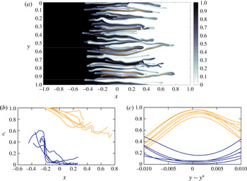
(a) Snapshot of the concentration profile at
 $t=1$
for a simulation with
 $Pe=16\,000$
and
 $R=2$
. Superimposed are lines which follow the peaks (orange) and troughs (blue) in concentration. (b) Concentration profile along peaks (orange) and troughs (blue). (c) Concentration profile in the transverse direction at
 $x=0$
centred around the peaks (orange) and troughs (blue).

One of the critical assumptions of the Koval model is that the concentration is either exactly one or exactly zero. We interrogate this assumption by plotting the concentration field from a simulation with a large Péclet number (
 $Pe=16\,000$
) in figure 7(a). We find that even at very large
 $Pe$
, the concentration is not just one or zero but varies in both the horizontal and vertical direction. The concentration along the local maxima and minima of the fingers (figure 7
b) decreases and increases towards the tips, respectively. In the transverse direction, the concentration takes on a single maximum or minimum in each finger, which, in its simplest form, can be approximated by a parabola (figure 7
c). These two factors together result in a much smaller prediction for the transverse variance in concentration than the simple Koval model predicts (figure 6
b). Interestingly, in this limit of large
 $Pe$
, the variance is independent of the Péclet number, which suggests that the Péclet number has no effect on the effective viscosity in this regime in agreement with the fact that (5.11) and (5.12) have no dependence on
 $Pe$
.
Motivated by these observations, we suggest a very simple improvement to the simple Koval model, which addresses one of its main assumptions. In the simple Koval model, the viscosity is uniformly given by
 $e^{R}$
or
 $1$
in each finger, which follows from the assumption of uniform concentration in each finger. However, we observe that the concentration actually varies across the fingers, and we can approximate this variation as being parabolic. In fact, the significant improvement to the simple model by the empirical fit (5.12) suggests that the main consequence of ignoring this variation is an inaccurate calculation of the effective viscosity. We therefore propose a simple modification of the Koval model in which the viscosity varies with a quadratic concentration profile across each finger; that is,
 $\unicode[STIX]{x1D707}(y)=\text{e}^{R(1-y^{2}/w_{f}^{2})}$
and
 $\unicode[STIX]{x1D707}(y)=\text{e}^{R(y^{2}/w_{b}^{2})}$
in the forward and backward propagating fingers, respectively. In all other respects, we retain the same assumptions as in the simple Koval model: the fingers are still assumed to be horizontally uniform, and to obtain a simple analytical solution with the same functional form as the simple Koval model, the mean concentration in each finger is still assumed to be either zero or one.
Under these assumptions, equation (5.9) instead becomes
 $$\begin{eqnarray}\displaystyle \frac{\unicode[STIX]{x2202}\overline{c}}{\unicode[STIX]{x2202}t}+\frac{\unicode[STIX]{x2202}}{\unicode[STIX]{x2202}x}\left(\frac{\unicode[STIX]{x1D702}_{f}\displaystyle \int _{-w_{f}}^{w_{f}}\text{e}^{R(1-y^{2}/w_{f}^{2})}\,\text{d}y}{\unicode[STIX]{x1D702}_{f}\displaystyle \int _{-w_{f}}^{w_{f}}\text{e}^{R(1-y^{2}/w_{f}^{2})}\,\text{d}y+\unicode[STIX]{x1D702}_{b}\int _{-w_{b}}^{w_{b}}\text{e}^{R(y^{2}/w_{b}^{2})}\,\text{d}y}-\overline{c}\right)=0. & & \displaystyle\end{eqnarray}$$
Combining (5.13) with the same constraints as before, and solving, results in the same expression for
 $\overline{c}$
as (5.11) but with an effective viscosity ratio
 $$\begin{eqnarray}\displaystyle M_{e}=\frac{e^{R}\text{erf}(\sqrt{R})}{\text{erfi}(\sqrt{R})}, & & \displaystyle\end{eqnarray}$$
where
 $\text{erfi}(x)$
is the imaginary error function. We denote this model as the ‘parabolic Koval’ model. As with the original Koval model, the effective viscosity does not depend on the width or the number of fingers.
Plot of the effective viscosity ratio measured for different values of
 $R$
and
 $Pe$
. Each point plotted is calculated by extracting the value of
 $M$
from a least-squares fit of (5.11) to the transversely averaged concentration profiles
 $\overline{c}(x,t)$
, at five different times
 $t=10,11,12,13,14$
and five different simulations. These measurements are then averaged and the error bars represent one standard deviation in these measurements. The three different model predictions are: simple Koval (blue, dashed), fitted Koval (green, dotted) and parabolic Koval (black, dot-dashed).

Figure 8 plots the effective viscosity ratio extracted from the numerical simulations (dots), together with the predictions of the simple Koval model (S-K), the empirically fit effective viscosity (F-K) (5.12) and the analytically derived model with parabolic transverse profiles (P-K) (5.14). The simple Koval model overpredicts the effective viscosity of the fingered region, whereas the parabolic model agrees well with both the empirical fit and numerical experiments. In fact, the parabolic model predicts smaller effective viscosities than the empirical fit for
 $R>3$
in qualitative agreement with experiments by Malhotra et al. (Reference Malhotra, Sharma and Lehman2015). Although the model agrees well with the data, it remains, of course, an approximation: it does not take into account the along-flow variations in concentration, and it still assumes the concentration (but not the viscosity) is either one or zero in each finger. Nevertheless, we have shown that an accurate effective viscosity in the Koval model can be derived simply by assuming the viscosity varies smoothly in the transverse direction. Accounting for the other approximations in the model is the subject of future work.
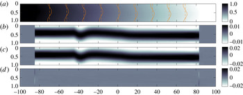
Snapshots at
 $t=500$
for
 $R=2$
,
 $Pe=2000$
. (a) Colour map of the concentration with overlaid contours of the raw (solid) and transversely averaged (dashed) concentration. (b) Colour map of
 $c^{\prime }(x,y)=c(x,y)-\overline{c}(x)$
. (c) Colour map of the horizontal velocity
 $u$
. (d) Colour map of the vertical velocity
 $v$
. Note that the
 $x$
-axis has been compressed by a factor of 10 in these plots.

6 Late times: single-finger exchange-flow regime
6.1 Numerical observations
At late times, we find a new flow regime which, to leading order, involves a single pair of fingers counter-propagating through a linear background concentration gradient as shown by the snapshots in figure 9. The concentration field is dominated by a nearly uniform background gradient in the horizontal direction with some small transverse deviations superimposed (figure 9
a). The concentration deviations (figure 9
b) are horizontally uniform and have a single maximum (i.e. they form a single finger). The horizontal velocity
 $u$
(figure 9
c) tracks closely the concentration deviations while the vertical velocity
 $v$
(figure 9
d) is only appreciable at the tips.
(a) Plot of the transversely averaged concentration. (b) Plot of the longitudinally averaged concentration
 $\overline{c}_{L}(y)=\int _{-\unicode[STIX]{x1D6E4}/2}^{\unicode[STIX]{x1D6E4}/2}c(x,y)\,\text{d}x=1/2+\int _{-\unicode[STIX]{x1D6E4}/2}^{\unicode[STIX]{x1D6E4}/2}c^{\prime }(x,y)\,\text{d}x$
. A sinusoidal fit for
 $t=150$
is given by the dashed black line. In both plots
 $R=2$
,
 $Pe=2000$
and the time, given by the colour, ranges from
 $150$
to
 $550$
.

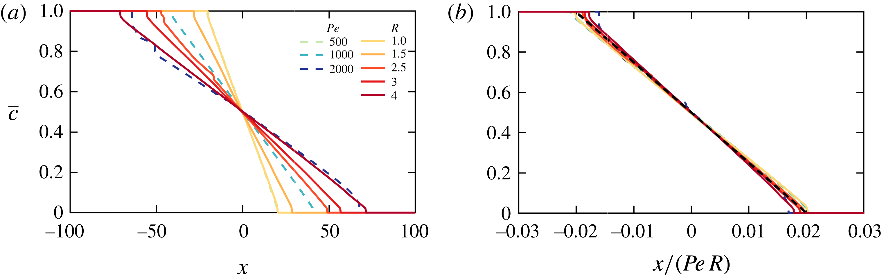
Figure 10 shows how the concentration field evolves over time. We find that the transversely averaged concentration,
 $\overline{c}(x)$
, is linear and steady in the interior. The fluid flow only widens the mixing region by filling in the linear profile (inset to figure 10
a). In addition, we find that
 $\overline{c}$
is no longer skewed and
 $\overline{c}=1/2$
is in the middle of the domain. These features are in stark contrast to the previous regime in which
 $\overline{c}(x)$
was asymmetric and nonlinear. Superimposed on this background concentration field are horizontally uniform deviations which are sinusoidal in the transverse direction (figure 10
b). These deviations decay in time, which ultimately results in a one-dimensional linear concentration field that evolves purely by diffusion in the
 $x$
direction.
We find that the single-finger state is stable, that is, no tip splitting occurs. The manner by which these fingers are stabilized is distinct from the classical Saffman–Taylor finger where surface tension acts as the stabilizing force. In this case, weak longitudinal concentration gradients and transverse diffusion not only stabilize the fingers but also cause them to decay.
6.2 Asymptotic model
The late-time regime is characterized by a linear background gradient with a single pair of counter-propagating fingers superimposed. The fingers have a very large aspect ratio, and so the velocity is given by (5.7), which for small deviations
 $c^{\prime }$
reduces to
 $$\begin{eqnarray}\displaystyle u=Rc^{\prime }+O(c^{\prime 2}). & & \displaystyle\end{eqnarray}$$
We look for a steady interior solution for
 $\overline{c}$
, for which (2.18) becomes
 $$\begin{eqnarray}\displaystyle \frac{1}{Pe}\frac{\unicode[STIX]{x2202}^{2}\overline{c}}{\unicode[STIX]{x2202}x^{2}}=O(c^{\prime 2}), & & \displaystyle\end{eqnarray}$$
or
 $$\begin{eqnarray}\displaystyle \overline{c}=-\unicode[STIX]{x1D6FC}x+{\textstyle \frac{1}{2}}+O(c^{\prime 2}). & & \displaystyle\end{eqnarray}$$
Given that the net change in concentration of the two fluids must be equal and opposite, the concentration at the mid-plane must be
 $1/2$
, which determines the constant of integration in (6.3).
Substituting the steady transversely averaged concentration (6.3) and velocity (6.1) into equation (2.19) results in a partial differential equation for the evolution of the deviations,
 $$\begin{eqnarray}\displaystyle \frac{\unicode[STIX]{x2202}c^{\prime }}{\unicode[STIX]{x2202}t}-\unicode[STIX]{x1D6FC}Rc^{\prime }=\frac{1}{Pe}\frac{\unicode[STIX]{x2202}^{2}c^{\prime }}{\unicode[STIX]{x2202}y^{2}}+O\left(\frac{c^{\prime }}{Peh^{2}}\right)+O(c^{\prime 2}). & & \displaystyle\end{eqnarray}$$
The leading-order behaviour of (6.4) is a balance between the growth/decay of the concentration deviations, advection of the background concentration gradient and transverse diffusion. Advection of the background tends to cause the deviations to grow since positive deviations tend to move high concentrations downstream (and negative deviations move low concentrations upstream), while diffusion causes them to attenuate. This competition results in the exponential decay of the fingers and eventual shutdown of the instability. Furthermore, this equation is independent of
 $x$
; therefore, the deviations must be horizontally uniform, as observed. The single-finger solution to the leading-order truncation of (6.4) is
 $$\begin{eqnarray}\displaystyle c^{\prime }(y,t)=\text{sin}(2\unicode[STIX]{x03C0}y)\text{e}^{-\unicode[STIX]{x1D6FE}(t-t^{\ast })}, & & \displaystyle\end{eqnarray}$$
where
 $t^{\ast }$
is a virtual origin relating to the transition between regimes and
 $$\begin{eqnarray}\displaystyle \unicode[STIX]{x1D6FE}=\frac{4\unicode[STIX]{x03C0}^{2}}{Pe}-\unicode[STIX]{x1D6FC}R. & & \displaystyle\end{eqnarray}$$
Note that, while a solution of (6.4) with any integer number of fingers is permissible, solutions with more fingers decay more rapidly over time, and the solution with
 $k=2\unicode[STIX]{x03C0}$
(6.5) is the slowest decaying mode.
The slope
 $\unicode[STIX]{x1D6FC}$
of the interior profile in (6.3) is set by the amount of mixing that occurs during the intermediate, nonlinear regime. That regime lasts for a time
 $t\sim O(Pe)$
during which the mixing zone grows linearly in time,
 $h\sim Rt$
. Therefore, once the system has reached the single-finger regime, the width of the mixing zone will have become
 $h\approx 1/\unicode[STIX]{x1D6FC}\sim RPe$
, such that
 $\unicode[STIX]{x1D6FC}R=\hat{A}/Pe$
, for some constant
 $\hat{A}$
. We fit
 $\hat{A}=24.9$
to the collapsed transversely averaged concentration profiles (figure 11
b).
We verify this model by measuring
 $\unicode[STIX]{x1D6FC}$
and
 $\unicode[STIX]{x1D6FE}$
from the numerical simulations. We calculate
 $\unicode[STIX]{x1D6FC}$
by measuring the slope of
 $\overline{c}$
at
 $x=0$
at some late time, and
 $\unicode[STIX]{x1D6FE}$
by measuring the decay rate of the maximum of
 $c^{\prime }$
at the mid-plane. Plots of the numerically measured
 $\unicode[STIX]{x1D6FE}$
and
 $\unicode[STIX]{x1D6FC}R$
are given in figure 12(a) and both quantities exhibit the predicted
 $1/Pe$
scaling. Finally, the validity of (6.6) is tested by plotting the ratio of
 $\unicode[STIX]{x1D6FE}$
measured from the simulations and
 $\unicode[STIX]{x1D6FE}(\unicode[STIX]{x1D6FC})$
calculated using (6.6). This quantity is plotted in figure 12(b) and deviates by a maximum of 4 % over a range of Péclet numbers and log-viscosity ratios.
(a) Plots of
 $\overline{c}(x)$
for
 $R=2$
,
 $Pe=500,1000,2000$
(dashed) and
 $Pe=1000$
and
 $R=1,1.5,2.5,3,4$
(solid) at
 $t=200$
. (b)
 $\overline{c}$
as a function of
 $x/(RPe)$
, with the fitted line
 $\overline{c}=1/2-24.9x/RPe$
(black, dashed).
(a) Plot of
 $\unicode[STIX]{x1D6FE}$
(circles) and
 $\unicode[STIX]{x1D6FC}R$
(diamonds) as functions of
 $Pe$
and
 $R$
(colours). (b) Ratio of
 $\unicode[STIX]{x1D6FE}$
, measured from the simulations as the decay rate of the maximum of
 $c^{\prime }$
at
 $x=0$
, to
 $\unicode[STIX]{x1D6FE}(\unicode[STIX]{x1D6FC}R)$
, calculated using (6.6) where
 $\unicode[STIX]{x1D6FC}$
is the slope of
 $\overline{c}$
measured at
 $t>200$
.

6.3 Total convective mixing
One of the major implications of this final single-finger exchange-flow regime is that the viscous-fingering instability can only generate a finite amount of convective mixing. In figure 13(a) we plot the time integral of the convective flux through the mid-plane,
 $$\begin{eqnarray}\displaystyle F=\int _{0}^{\infty }\int _{0}^{1}uc^{\prime }|_{x=0}\,\text{d}y\,\text{d}t, & & \displaystyle\end{eqnarray}$$
as a function of the Péclet number and log-viscosity ratio. We find that the flux increases linearly with both
 $Pe$
and
 $R$
for
 $Pe\gg 1$
, and can be fit by the functional form
 $F=\hat{a}R(Pe-\hat{b}/R)$
, where the shift in the Péclet number,
 $\hat{b}/R$
, corresponds to the onset of the instability as described in § 5.1. We find that the numerical data are best fit with
 $\hat{a}=5.3\times 10^{-3}$
and
 $\hat{b}=45$
(solid lines in figure 13
a).
Of course, provided advection dominates the horizontal transport, the quantity
 $F$
can also be directly related to the slope
 $\unicode[STIX]{x1D6FC}$
of the late-time profiles, by mass conservation. Such a balance gives
 $$\begin{eqnarray}\displaystyle F\approx \int _{0}^{\infty }\bar{c}\,\text{d}x\approx \frac{1}{8\unicode[STIX]{x1D6FC}}. & & \displaystyle\end{eqnarray}$$
For the three values of
 $R$
plotted, we find that this prediction gives good agreement for
 $Pe>O(100)$
(figure 13
b), which suggests that for the range of
 $R$
plotted, horizontal diffusion plays a negligible role in mixing for
 $Pe>O(100)$
.
(a) Time-integrated convective exchange flux
 $F$
(6.7) between the two fluids as a function of
 $Pe$
and
 $R$
(colours), as calculated from the numerical simulations. In order to calculate the infinite time integral in (6.7), we integrate the numerical data out to
 $t=200$
, which is well into the late-time regime in all simulations, and fit a decaying exponential function
 $E(t)$
to the flux
 $\int _{0}^{1}uc^{\prime }|_{x=0}\,\text{d}y$
for subsequent times such that
 $F=\int _{0}^{200}\int _{0}^{1}uc^{\prime }|_{x=0}\,\text{d}y\,\text{d}t+\int _{200}^{\infty }E(t)\,\text{d}t$
. The lines of best fit (black) correspond to the fit
 $F=5.3\times 10^{-3}R(Pe-45/R)$
. (b) Ratio of the time-integrated convective exchange flux and the final slope of the transversely averaged concentration.

7 Discussion and conclusions
In this paper, we have investigated miscible viscous fingering in a semi-infinite planar geometry using high-resolution simulations. We identified three distinct regimes: an early-time linearly unstable regime, an intermediate-time nonlinear regime and a late-time single-finger exchange-flow regime. In each of these regimes, we identify the predominant balances and scalings for the mixing length
 $h$
, the number of fingers
 $n$
and the total convective transport
 $Nu$
(table 1).
The dimensional characteristic length scales of the flow structures are summarized in table 2. The early-time fingering dynamics are set by a local balance of advection and diffusion at the finger scale and hence are independent of the width of the porous medium
 $a$
. The flow is more unstable – that is, the flow has finer structures and faster growth rates – when the viscosity contrast and velocity are large, or the diffusivity is small. The fingers then spread longitudinally while coarsening, also independent of the width of the porous medium. Finally, once the instability has had enough time to diffuse transversely across the entire width of the porous medium, which occurs at a time scale
 $T\sim a^{2}/D$
, the flow enters the late-time regime. In this case, a single pair of counter-propagating fingers remain, which occupy half of the width of the domain respectively.
Dimensional length scales
 $X$
and
 $Y$
as a function of dimensional time
 $T$
. The transition from the early-time to intermediate-time regime occurs at
 $T\sim O(\unicode[STIX]{x1D719}^{2}D/R^{2}U^{2})$
and the transition from the intermediate-time to late-time regime occurs at
 $T\sim O(a^{2}/D)$
. The vertical length scale in the intermediate regime first grows advectively, then diffusively, as discussed in § 4.1.

In § 5.1, we showed that for sufficiently small Péclet numbers, the flow can skip the intermediate regime, and for even smaller Péclet numbers, the instability can be suppressed altogether. We then presented a linear stability analysis to identify this cutoff for the instability and compared it to numerical experiments.
In § 5.2 we derived an improvement on current models for the transversely averaged concentration in the intermediate-time nonlinear regime. We started by reproducing the simple Koval model, identified where it disagreed with the numerical simulations and improved on one of its shortcomings by including a simple model of the nearly parabolic concentration profile across propagating fingers. We used this ansatz to derive the effective viscosity of the fingered region (5.13), in good agreement with both the numerical simulations and the empirical fit to the Koval model.
Finally, in § 6 we identified a new late-time single-finger exchange-flow regime in which the flow consists of a linear background gradient and counter-propagating fingers. These fingers exponentially decay and convection stops leaving a linear background gradient. We derived a model for the asymptotic behaviour and showed that it agrees with the numerical simulations. One important consequence of this eventual shutdown is that there is a maximum amount of convective mixing that the instability can generate. Since diffusion coefficients for typical pairs of fluids tend to be very small, this shutdown is most relevant when the displacement process occurs at very small scales (small
 $a$
) or very long times.
To illustrate the relevant length and time scales in the late-time regime, we use parameter values from the
 $\text{CO}_{2}$
sequestration project at Sleipner to estimate the ‘shutdown time’,
 $T_{sd}$
, taken to reach the late-time regime and the ‘final’ mixing zone width
 $H$
. We take the parameter values of the carbon-dioxide/brine system to be as follows (Neufeld et al.
Reference Neufeld, Hesse, Riaz, Hallworth, Tchelepi and Huppert2010; Boait et al.
Reference Boait, White, Bickle, Chadwick, Neufeld and Huppert2012): background velocity, which is the buoyancy velocity,
 $U=4\times 10^{-6}~\text{m}~\text{s}^{-1}$
; log-viscosity ratio
 $R=2.5$
; porosity
 $\unicode[STIX]{x1D719}=0.3$
; aquifer thickness
 $a=10~\text{m}$
; and diffusivity
 $D=2\times 10^{-9}~\text{m}^{2}~\text{s}^{-1}$
. In this case, the diffusivity is taken to be the molecular diffusivity of carbon dioxide and brine
 $D_{m}$
. Note that this is only valid when the pore-scale Péclet number, defined as
 $Ua_{p}/D_{m}$
(
 $a_{p}$
is the size of the pores), is small; otherwise the effective diffusivity is given by an anisotropic velocity-dependent dispersion tensor that could be significantly larger than
 $D_{m}$
(Lake Reference Lake1989).
Using these parameters, the Péclet number of the flow is
 $Pe=7\times 10^{4}$
. The time until shutdown can be approximated from the numerical simulations as
 $T_{sd}\approx 10^{-1}a^{2}/D$
which gives a shutdown time of approximately
 $150$
years. Furthermore, the mixing zone can be approximated as
 $H=10^{-1.5}Ra^{2}U/\unicode[STIX]{x1D719}D$
which gives a 50 km long mixing zone upon shutdown. In contrast, if the interface were stable and the mixing at the interface only occurred through diffusion, the width of the mixing zone would grow like
 $\sqrt{4Dt}$
, which, after
 $150$
years, would be approximately 5 m.
In a real porous medium, some of the assumptions we made during the analysis may no longer hold. For instance, the dispersion can be anisotropic and viscosity or velocity dependent; the permeability often varies spatially at a variety of length scales (pore scale to field scale) and with varying degrees of randomness (from completely random to highly structured); and the fluids can be only partially miscible. While some of these topics have been discussed in the context of the onset problem and early-time behaviour (Zimmerman & Homsy Reference Zimmerman and Homsy1991, Reference Zimmerman and Homsy1992; Tan & Homsy Reference Tan and Homsy1992; De Wit & Homsy Reference De Wit and Homsy1997a ,Reference De Wit and Homsy b ; Nicolaides et al. Reference Nicolaides, Jha, Cueto-Felgueroso and Juanes2015), their impact on the late-time behaviour remains to be understood.
Acknowledgements
J.S.N. is supported by a Gates Cambridge Scholarship, D.R.H. is supported by a Research Fellowship at Gonville and Caius College, Cambridge and J.A.N. is partly supported by a Royal Society University Research Fellowship.