4.1 Shear layer coupling

As mentioned above, the averaged trajectory of $\tilde{E}_{max}$ for each section was used to define the locations where the hot-wire measurements were obtained. The hot-wire data from these trajectories reveal details about the spectral content within the shear layer. For each case, the two hot-wire probes were mechanically traversed along the mean shear layer trajectories. Figure 9 shows a sample of the power spectra for both sections (5 : 1 and 1 : 1) at two different positions along the shear layer. For both bodies, the lighter curve shows the power spectrum of the hot-wire probe taken directly adjacent to the leading edge, where the origin is defined using the PIV system as the leading edge corner. The hot-wire system thus is inherently offset in order to avoid a collision of the probe. Near the leading edge, the spectra in both cases appear to have most of their energy concentrated toward the low-frequency end with a discrete concentration at the wake shedding frequency labelled $f_{VK}$ . Comparing the two sections, the 1 : 1 section has much more energy at $f_{VK}$ due to the flapping of the fully separated shear layer. The spectra of the 5 : 1 section have less energy at the wake shedding frequency, which is a further evidence that the wake’s influence is smaller for this section. At some small but finite distance along the shear layer, at $(x/h,y/h)=(0.174,-0.190)$ and (0.081, $-$ 0.100) for the 5 : 1 and 1 : 1 sections respectively, the spectra change dramatically. In both cases a high frequency, with a broad banded peak, rises up several orders of magnitude compared to the signals taken upstream at the corner. This high-frequency content is labelled as $f_{KH}$ . Although its precise spatial definition is not easily described, as will be discussed in later sections, it is pointed out here qualitatively. One highlight is that, depending on the area of interest, there may be multiple competing modes, and the relative amplitude between $f_{VK}$ and $f_{KH}$ is one metric to evaluate the level of coupling between activity occurring in the wake and the KH instability originating at the leading edge.

Figure 9.

Power spectra taken at the leading edge corner $(x/h,y/h)=(0,0)$ , and at $(x/h,y/h)=(a)(0.174,-0.190)$ for the 5 : 1, and (b) (0.081, $-$ 0.100) for the 1 : 1 sections. $Re_{h}=3.04\times 10^{4}$ .

Another way to quantify the level of coupling between the wake and shear layer regions is through cross-correlations using two hot-wire signals. Two-point measurements have been used by investigators in incompressible flows to extract details about features such as physical size, frequency and convective speed (Tennekes & Lumley Reference Tennekes and Lumley1972). Traditionally, two probes are separated in space and the cross-correlation function is calculated using the two simultaneously acquired signals normalized by the product of their standard deviations,

(4.3) $$\begin{eqnarray}\displaystyle \unicode[STIX]{x1D70C}(\unicode[STIX]{x0394}x,\unicode[STIX]{x0394}y,t)={\displaystyle \frac{u_{mag,\,1}^{\prime }(x,y,t)\,u_{mag,\,2}^{\prime }(x+\unicode[STIX]{x0394}x,y+\unicode[STIX]{x0394}y,t)}{\sqrt{\overline{{u^{\prime }}^{2}}_{mag,\,1}}\,\sqrt{\overline{{u^{\prime }}^{2}}_{mag,\,2}}}}. & & \displaystyle\end{eqnarray}$$

Figure 10.

Cross-correlation coefficients along the length of the three sections. Direction of increasing $\unicode[STIX]{x0394}x$ is indicated in the upper centre portion of the figure. $Re_{h}=3.04\times 10^{4}$ .

In this case, the two signals are velocity magnitudes measured by the hot-wires. As seen in (4.3), the value of $\unicode[STIX]{x1D70C}$ is dimensionless, decaying with increasing separation distance at zero time shift from $\unicode[STIX]{x1D70C}(0,0,0)=1$ according to Schwartz’s inequality for stationary signals. Since the wires must maintain a small separation distance in order to avoid collision, the resulting coefficient can only approach unity at small distances $\unicode[STIX]{x0394}x$ , $\unicode[STIX]{x0394}y$ . Here, the two hot-wire probes were placed on the shear layers’ average trajectory with a single wire fixed in the plane of the trailing edge and the other was traversed along the previously mentioned trajectory of maximum TKE, in the direction upstream of the fixed probe. The cross-correlation coefficients were found as a function of $\unicode[STIX]{x0394}x/h$ or the distance upstream from the fixed probe, and are presented in figure 10. As can be seen in the figure, the correlation coefficient for each body is close to unity when the probes are very close to each other in the wake, as one might expect since the probes are at their closest. As the travelling probe was traverses upstream along the shear layer, i.e. increasing $\unicode[STIX]{x0394}x/h$ , the correlation coefficients decrease as the distance between probes increased. Note that here, the sign of $\unicode[STIX]{x0394}x$ is inverted in comparison to $x$ , which is a necessary arrangement to distinguish between convective and global instabilities. Aligning the two probes at the trailing edge and moving one upstream tracks the upstream influence of global instabilities only, since convective instabilities are directional and thus depend on the convective speeds and times in the flow. Moving the travelling probe upstream from that initial location and extracting the correlation value at zero time lag then documents how far upstream the global behaviour of the VK instability extends at a given instant in time.

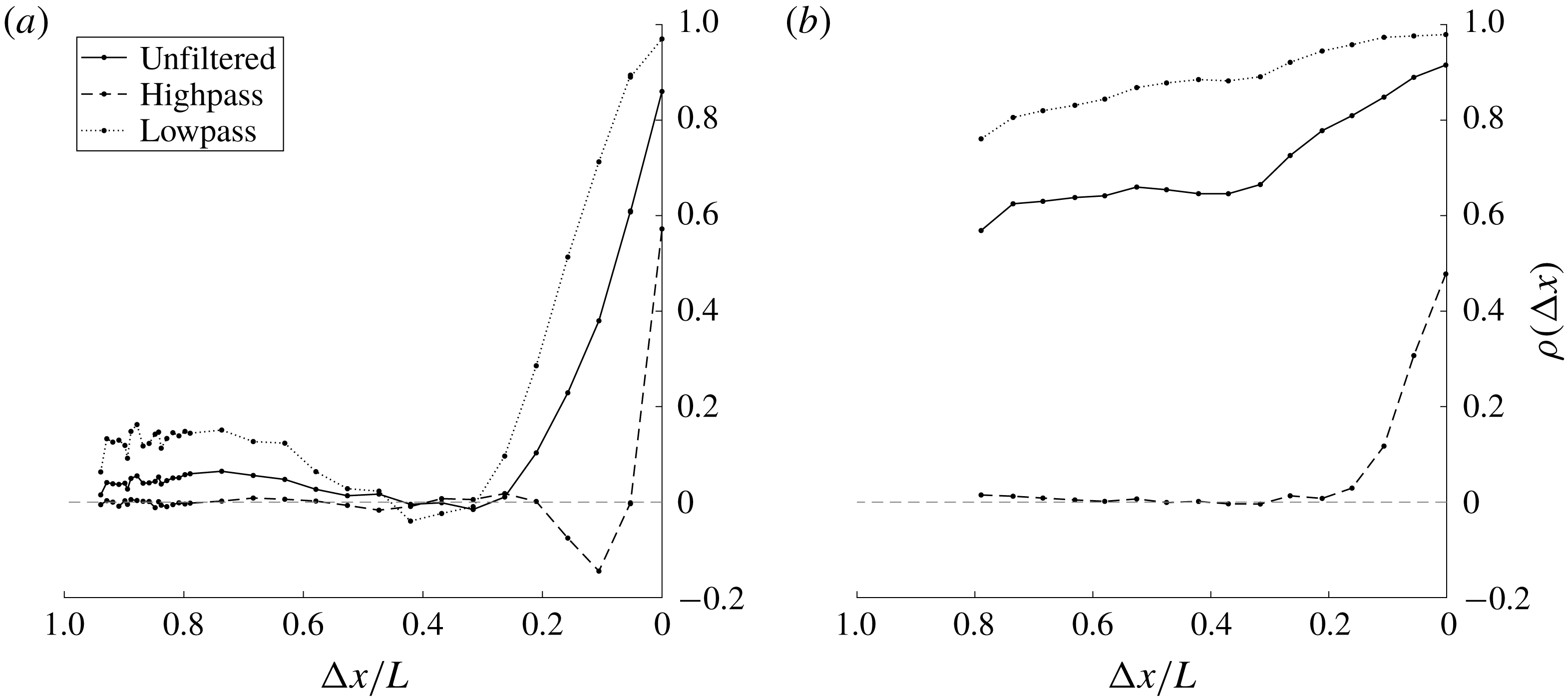
For the 1 : 1 section, the correlation coefficient remains above 50 % everywhere along the shear layer, indicating a relatively high level of correlation, suggesting that the wake’s influence is significant all the way to the leading edge. Sections with extended afterbodies such as the 3 : 1 and 5 : 1, show correlation coefficients continuing to decay with upstream distance for more than one body height upstream. The 5 : 1 section in particular is nearly zero near the leading edge, demonstrating that the two probes experience two independent and uncorrelated signals. As such, it may be expected that the wake’s influence is significantly smaller for the 5 : 1 section than for the 1 : 1 section.

Figure 11 presents the spatial correlations with hot-wire signals filtered before the correlation coefficient was calculated. When the high pass filter (with a cutoff frequency at $fh/U_{\infty }=0.39$ , nearly $3.5$ times the Strouhal number, $St$ ) was applied, the coefficients reflect the correlation associated with shear layer content only. In the case of the 1 : 1 square section (figure 11 b), the high pass filter shows no correlation between the signals at leading and trailing edges. Low pass filtering at the same cutoff frequency has the opposite effect. Isolating low-frequency content associated with the wake shedding raises coefficients, demonstrating an increased global coherence, a direct result of the upstream propagation of instability waves associated with the wake instability. This is most clearly seen with the 1 : 1 square. In addition to a net offset of increased coherence for all measured locations, the differences between leading and trailing edge are reduced for the low pass filtered data in comparison to the highpass filtered data. Physically, this points toward the low-frequency dominance associated with the global instability from wake shedding. In either case, it is clear that there are two primary frequency components, the first being low frequencies that appear to be coherent, meaning their correlation coefficients extend far upstream from their source. The second component is the high frequency shear layer content, less correlated over the length of the shear layer. Of these, the low and high-frequency regimes appear to be less coupled for the 5 : 1 section, as shown by the lack of correlation at the leading edge of the 5 : 1 section (figure 11 a). Therefore, the interactions between the two modes of instability are examined primarily through the use of the 5 : 1 section as the two modes are more independent of one another. All sections, however, display clearly that the shear layers’ frequency content is heavily dependent on the spatial location. That spatial dependence also includes Reynolds number effects as will be discussed in the next section.

Figure 11.

Highpass and lowpass filtered correlations for (a) the 5 : 1 section, and (b) the 1 : 1 square section. Sign conventions are same as figure 10.

4.2 Reynolds number dependency

Figure 12 shows the dependence of the shear layer frequency on Reynolds number for the sections tested. Figure 12(a–c) presents the Strouhal number, $St=f_{VK}h/U_{\infty }$ for the 1 : 1, 3 : 1 and 5 : 1 sections, respectively, over Reynolds numbers. For each section, the Strouhal number is nearly constant over a wide range of Reynolds numbers. This Reynolds number invariance is attributed to a linear correspondence between the vortex shedding frequency in the wake, $f_{VK}$ , and the free-stream velocity, $U_{\infty }$ . In figure 12(d) the variation of the ratio of the shear layer’s frequency to the wake’s frequency, $f_{KH}/f_{VK}$ , with Reynolds number is shown along with data from relevant literature. It is immediately obvious that the shear layer’s frequency does not vary linearly with wind speed (assuming a common reference length for the Reynolds numbers). Instead, the curves abide by a power law relationship, $Re^{n}$ , with exponents ranging upwards from $n=0.5$ as first noted by Bloor (Reference Bloor1964). The best-fit value of $n$ is given a physical justification for a circular prism ( $n=0.67$ ) in Prasad & Williamson (Reference Prasad and Williamson1997) and extended to the square prism ( $n=0.60$ ) in Lander et al. (Reference Lander, Moore, Letchford and Amitay2018). It is interesting that all geometries fit well with a power law; however, both the exponent and the coefficient are different for each prism geometry. These differences may be explained by considering the dynamics at separation for each body. For any geometry, the shedding frequency of the KH events near separation ought to scale inversely with the thickness of the separating boundary layer. In zero or adverse pressure gradients, such as the separation point on a circular prism, the thickness is larger than that of a boundary layer separating under an highly favourable pressure gradient such as the front face of a square prism. This reduction in boundary layer thickness may explain the initial offset of each of the curves. It is precisely these intricacies of the shear layer, with a shared dependence on spatial coordinate and free-stream Reynolds number, that provoke the curiosity of the authors and warrant a deeper investigation into their natural behaviour.

Figure 12.

Variation of the Strouhal number with Reynolds number for the (a) 1 : 1, (b) 3 : 1 and (c) 5 : 1 sections. (d) The dependence of $f_{KH}/f_{VK}$ with Reynolds number.

The data in previous sections have demonstrated the quantities of a separated shear layer that change significantly in space as well as with respect to Reynolds number. These dependencies are important when analysing shear layer behaviour as the relevant scales are not as predictable as those observed in the wake. Particular attention is noted for the leading edge corner where the spatial dependence is critical to understand the early stages of transition to turbulence. This region, which is founded qualitatively on the regimes in figure 1, is partially summarized in figure 13. Figure 13 shows the spatio-temporal dependence of the bluff body’s shear layer using both PIV and hot-wire. On the left-hand side, an instantaneous normalized spanwise vorticity field ( $\overline{\unicode[STIX]{x1D714}}_{z}>20$ ) is displayed near the leading edge corner of the 1 : 1 square section as a way to visualize the transition process. As a reference for the spatial extent of the image, the domain here is 0.84 $h$ and 0.34 $h$ in $x$ and $y$ directions, respectively.

Figure 13.

An instantaneous vorticity field (a), and sample time histories and a reference length equal to one period of $f_{VK}$ (b) around the leading edge corner of a 1 : 1 (square) prism, $Re_{h}=3.04\times 10^{4}$ . Saturation level is set to $\overline{\unicode[STIX]{x1D714}}_{z}=20.$

In the figure, a laminar shear layer is detected immediately after separation, near point A, similar to the results in figure 4. The shear layer quickly bends into the direction of the mean flow (left to right in the figure) and eventually rolls up in a counter-clockwise direction forming a laminar vortex, which can be detected near point E. Downstream of the vortex formation, vortex pairing can be detected, followed by a breakdown of the organized structures to smaller turbulent eddies. On the right hand side, five time traces are shown, one for each of the points labelled in the vorticity field. Initially, at point A, only one frequency can be seen, namely the $f_{VK}$ . This time trace is directly taken from time history used for the calculation of the power spectra in figure 9. Note that the $f_{KH}$ frequency is not detected at this location, suggesting either the disturbance amplitude is below the resolution of the probe, or that the local Reynolds number is below the critical Reynolds number for transition to initiate. At point B, a much higher frequency can be observed as a small bursting event, intermittently spaced on the von Kármán signature. Point C shows the same high-frequency content becoming less intermittent. These are the early stages of shear layer transition (i.e. growth of disturbances) and the accumulation of energy at $f_{KH}$ . Points B–D show the evolution of $f_{KH}$ as it grows in space along the shear layer and culminating at point E, where formation of a vortex marks the end of the linear growth. In essence, this sequence demonstrates how short the region is where linear growth of the shear layer instabilities is likely to be found.

With a physical intuition established, we now shift to focus on comparing metrics and trends already established in the literature. The nonlinear Reynolds number dependencies within the shear layer behaviour were discussed with regard to the appropriate length scale in Bloor (Reference Bloor1964), as well as the corresponding time scales (Prasad & Williamson Reference Prasad and Williamson1997) and the combination of scales was then satisfied using the linear scaling in Lander et al. (Reference Lander, Moore, Letchford and Amitay2018) who also noted that a thinning boundary layer on the front face of the section mirrors the behaviour of shear layer transition lengths. In the following paragraphs it will further be shown that upon reducing the wake’s influence, the spatial amplification of disturbances reveals its own Reynolds number dependency. This is supportive of the idea that the shear layer behaves more similar to what may be expected of a boundary layer on the front face of the section, rather than an inviscid planar mixing layer alongside it. With these new details, a more comprehensive view of the bluff body shear layer arises, encouraging a holistic view of the bluff body flow field.

Unlike the planar mixing layer, the bluff body shear layer experiences external influences including intense curvature, potential viscous effects due to the proximity to a solid surface, and proximity to other instability modes. These factors serve to elevate growth rates and obscure comparisons made with the planar mixing layer literature. For example, the mixing layer behind a backward facing step was found to grow at two different rates according to Sato (Reference Sato1956), as well as experiments downstream of a splitter plate in Winant & Browand (Reference Winant and Browand1974). The junction between the two growth rates marked a transition point for a free shear layer with infinite boundary conditions. However, Lander et al. (Reference Lander, Moore, Letchford and Amitay2018) used a similar analysis for the 2-D square prism that showed a continuous distribution of momentum thickness both upstream and downstream of what is later defined as the transition point for the square prism. Extending that analysis, the shear layer width is defined in the current study using the momentum thickness found in Fiedler (Reference Fiedler1991), whose definition accounts for recirculating flows in local coordinates.

(4.4) $$\begin{eqnarray}\displaystyle \unicode[STIX]{x1D703}(s)=\int _{y_{1}^{\prime }}^{y_{2}^{\prime }}\left({\displaystyle \frac{\overline{U}_{s}(s,y^{\prime })-\overline{U}_{s,min}}{\overline{U}_{s,max}-\overline{U}_{s,min}}}\right)\left(1-{\displaystyle \frac{\overline{U}_{s}(s,y^{\prime })-\overline{U}_{s,min}}{\overline{U}_{s,max}-\overline{U}_{s,min}}}\right)\text{d}y^{\prime }. & & \displaystyle\end{eqnarray}$$

Schematics and representative profiles illustrating this transformation are given in Lander et al. (Reference Lander, Moore, Letchford and Amitay2018). The variable $y^{\prime }$ corresponds to the direction normal to the shear layer’s trajectory at each streamwise coordinate. The slope of that line is inversely proportional to the tangent angle of the shear layer trajectory, and approaches a Cartesian grid when the shear layer becomes aligned with the free stream. The variable, $s$ , is the arc-length distance along the shear layer, and $\overline{U}_{s}$ is then the mean velocity in the local direction of the shear layer axis. Limits $y_{1}$ and $y_{2}$ correspond to the locations where $\overline{U}_{s,max}$ and $\overline{U}_{s,min}$ are found. The resulting local alignment allows for the calculation of a host of lengths and velocities that are skewed when described using traditional Cartesian coordinates. By aligning with streamlines or main gradients in the flow, a curved shear layer can be geometrically unwrapped, ignoring any effect of the pressure field. In doing so, it appears that the main functionality so far has been to compare curved shear layers with the archetypal planar mixing layer scenario. The result, as mentioned above, is that growth rates of shear layers born from leading edge separation are substantially higher and continuous functions of the axial coordinate. The present study confirms the elevated growth rates for all sections tested.

Figures 14(a) and 14(b) show the momentum thickness distributions for the 5 : 1 and 1 : 1 sections near the leading edge, respectively. In both cases, the coordinate system is local to the time-averaged shear layer position. The use of local coordinates is limited here to a single figure for comparison and validation purposes. In the figure, the continuously increasing nature of $\unicode[STIX]{x1D703}$ is clear in all cases. Focusing on figure 14(b), two curves from the present study are compared to similar Reynolds number cases explored by Lander et al. (Reference Lander, Moore, Letchford and Amitay2018). Data with similar Reynolds numbers for the 1 : 1 section match reasonably well. At higher Reynolds numbers, the agreement is better between the two data sets. At lower Reynolds numbers, there are differences in the two experiments beyond $s/h=0.3$ , which may be due to the differences in blockage ratios between the two experiments, 9.1 % and 6.3 %, the later of the two corresponding to the current study. It is worth noting that, while not included here, a similar treatment of direct numerical simulation (DNS) data shown in that work at $Re_{h}=2.2\times 10^{4}$ from Trias, Gorobets & Oliva (Reference Trias, Gorobets and Oliva2015) falls between curves of the present study at $Re_{h}=1.34\times 10^{4}$ and Lander’s data at $Re_{h}=1.67\times 10^{4}$ . For the 5 : 1 section (figure 14 a), the shear layer evolution with Reynolds numbers is more compelling. As Reynolds number increases the magnitude of the exponent of a line of best fit, $\unicode[STIX]{x1D703}\propto A\times (s/h)^{B}$ , decreases bringing the growth of the momentum thickness closer to a linear trend. Values extracted from a simple curve fitting procedure are listed in table 2.

The differences in shear layer development are more easily differentiated in the case of the 5 : 1 section. It appears that the reduced levels of coupling on the longer section more easily distinguish the true growth of the shear layer instability rather than the growth of a combination of instabilities as in the 1 : 1 body. This detail marks a departure from Lander’s work on the square prism. Nevertheless, all distributions of momentum thickness measured in the current study are continuous, meaning that they lack the necessary change in slope needed to identify a transition point. However, the apparent transition as seen through the hot-wire, and instantaneously through PIV, can be properly tracked through a different parameter, namely the turbulent kinetic energy, $\tilde{E}$ . What is appealing about $\tilde{E}$ , as initially reported in Lander et al. (Reference Lander, Moore, Letchford and Amitay2018), is that while the locus of the maxima was shown in figure 8 to be invariant with respect to Reynolds number, it will now be shown that the content of those points possess a strong dependency on Reynolds number, strong enough to form the basis for transition lengths of many rectangular sections.

Figure 14.

Variation of the momentum thickness with the normalized arc-length distance along the shear layer axis for (a) 5 : 1 section, and (b) 1 : 1 section at two different Reynolds numbers compared to data from Lander et al. (Reference Lander, Moore, Letchford and Amitay2018). Every other point is plotted.

Table 2.

Curve fitting coefficients for momentum thickness of the separated shear layer. Values are given as low/high where $Re_{low}/Re_{high}$ corresponds to $1.34\times 10^{4}/1.18\times 10^{5}.$ Values apply to $0<s/h<0.5$ .

The effect of Reynolds number on the distribution of $\tilde{E}_{max}$ along the 5 : 1 section for three different Reynolds numbers is presented in figure 15. Each of the three curves demonstrates qualitatively similar behaviour. Near the leading edge corner, each of the curves begins from a low free-stream value and subsequently rises with an exponential trend until it saturates. Beyond those saturation points the curves decay slightly and change gradually beyond $x/h=1$ , where at the trailing edge the curves converge. The increase near the leading edge is what is most convincing about this particular data set. Increasing the Reynolds number has several important effects on $\tilde{E}_{max}$ . The following observations are common to all section types and Reynolds numbers tested but for brevity are plotted here only for the 5 : 1 section. First, the initial values of $\tilde{E}_{max}$ climb approximately linearly with respect to increasing $Re_{h}$ . Their magnitudes are of the order of 1 % of the energy of the free stream. Second, the exponential rises of the turbulent kinetic energy are increasingly more aggressive, a feature that becomes much more vivid for longer sections such as the one in figure 15. While PIV cannot distinguish which frequencies grow faster than others, steeper exponential curves with increasing $Re_{h}$ here are qualitatively synonymous with elevated spatial growth rates of a band of unstable frequencies. Ultimately, the curves of $\tilde{E}_{max}$ saturate of the order of 5 %–10 % of the energy of the free stream at which point they have overstepped the notion of linear superposition on the mean flow. The level at which $\tilde{E}_{max}$ saturates steadily decreases as Reynolds number increases, and the saturation location moves upstream with diminishing gains. These features are in line with those involving viscous instabilities where the distance to transition is described using a local Reynolds number, $Re_{x}$ . As the free-stream Reynolds number increases, the distance to the critical local Reynolds number is reduced, resulting in shorter transition lengths.

A Reynolds-dependent transition process in a nominally separated flow raises interesting questions as to the exact origins of the observed instability. Specifically, one may question whether or not the observed trends are simply downstream artefacts of front face boundary layer activity undergoing viscous instability, or if the presence of the corner is close enough to contribute wall effects. Previous work on the square prism by this same group found spatial amplification rates that appeared to be constant over the Reynolds numbers tested; however, figure 15 indicates otherwise. Returning to the time-averaged positions of the shear layers in figure 8, the trajectories over the first half-body dimension are nearly the same suggesting that the proximity of the wall cannot explain the apparent presence of such effects for the 5 : 1 section. Nevertheless, these traits using $\tilde{E}_{max}$ constitute the beginnings of a transition length for separated shear layers of rectangular sections. However, the extent of Reynolds number dependency appears to be short lived. Beyond the saturation of $\tilde{E}_{max}$ the curves slowly converge onto one another giving a hint of self-similarity near the trailing edge.

Figure 16 show profiles of $\tilde{E}$ on a normalized vertical coordinate, $y^{\ast }=y-y|_{\tilde{E}_{max}}$ for the same three Reynolds numbers, demonstrating a lack of similarity near the leading edge but a convincing self-similar profile near the trailing edge. In figure 16(a), the profiles are presented at $x/h=0.15$ , which is beyond the saturation point for high Reynolds numbers and upstream of the saturation for the lower Reynolds numbers. As a result, the profiles’ peak magnitudes are not easily sorted by Reynolds number at first glance. At the highest Reynolds number of $Re_{h}=1.18\times 10^{5}$ , the maximum $\tilde{E}$ is between the lower two Reynolds number curves, a feature that is easily distinguished in figure 15. As can be seen in figure 16(b), at $x/h=4.5$ all three profiles collapse on top of one other, suggesting Reynolds number independence near the trailing edge. This independence might be due to the proximity to the wake, which is governed by an inviscid mechanism, as seen by the Strouhal number behaviour. Figures 15, 16 and 13 indicate a rapid transition process, which can be quantified and verified through $\tilde{E}$ .

Figure 15.

Downstream trajectories of $\tilde{E}_{max}$ . A 95 % confidence interval is shown for $Re_{h}=1.34\times 10^{4}$ only. Every tenth point is plotted.

Figure 16.

(a) Wall-normal profiles of $\tilde{E}$ at (a) $x/h=0.15$ , and (b) at $x/h=4.5$ . Every fifth point plotted.

Another way to visualize the spatial development of transition within the separated shear layer is through analysis of instantaneous fields. Figure 17(a,c) and figure 17(b,d) show contours of instantaneous spanwise vorticity, $\overline{\unicode[STIX]{x1D714}}_{z}$ , near the leading edge of the 5 : 1 and 1 : 1 sections, respectively. Figure 17(a) shows a band of vorticity stemming from the leading edge of the 5 : 1 section, similar to the distribution in figure 13 where the Reynolds number is moderate, $Re_{h}=1.34\times 10^{4}$ . At an order of magnitude higher Reynolds number ( $Re_{h}=1.18\times 10^{5}$ , figure 17 c), the same pattern is visible although the downstream location where the first vortex is detected is substantially closer to the leading edge and the size of the resulting structure is smaller. Similarly, the 1 : 1 section show the same main features, where at the lower Reynolds number (figure 17 b) there is a significant distance to the roll up event, while at the higher Reynolds number case (figure 17 d) the roll up of the first vortex is very close to the leading edge. In contrast to much of the mean flow parameters discussed earlier, there is a striking dependence on the Reynolds number. Indeed, the vorticity fields displayed here are common to the tens of thousands of instantaneous fields captured over the course of the experimental campaign, indicating that this behaviour is predictable although its exact coordinates vary slightly in space. Furthermore, it is shown here that while the position of the separated shear layer is nearly Reynolds number independent, its unsteady content is not. This notion can be observed by aligning these vorticity fields with the corresponding magnitudes of $\tilde{E}_{max}$ as done in figure 17(e) for the 5 : 1 section and figure 17(f) for the 1 : 1 square section. This pattern in the instantaneous fields in figure 17 is similar to that highlighted in Lander (Reference Lander2017), who used the ${\mathcal{Q}}$ criterion to identify the first coherent structure in the shear layer and noted their alignment with an integrated kinetic energy parameter for the square prism. Here it is shown that a similar analysis can readily be extended to other rectangular sections with improving resolution as the influence of the wake is diminished with increasing aspect ratio. While earlier discussions appealed to the position of the maximum TKE, its magnitude is now shown to be a useful tool to detect the location of discrete vortex formation and the end of the linear growth of the instability. In fact, the instantaneous vorticity plots show that the roll up of the vortex coincides nicely with the saturation of $\tilde{E}_{max}$ along the $x$ axis for the 5 : 1 section. A similar pattern applies for the 1 : 1 square section in figure 17(f), although the initial levels of $\tilde{E}_{max}$ are higher, the slopes apparently similar to one another, and instead of a saturation the distributions experience a slope reduction that coincides in space with the location of the first vortex. Note that since the shear layer associated with the 1 : 1 section is significantly affected by the proximity to the wake, $\tilde{E}_{max}$ continues to increase. Appealing once again to linear theory, one might expect to see exponential growth regions of the shear layer where the growth rates are best described using linear methods. The slope reduction in 17(f) is likely where the disturbance growth is at first linear but quickly goes nonlinear and is dominated by the growth of another instability in the flow, namely the instability in the wake.

Figure 17.

Instantaneous vorticity fields. (a,c) 5 : 1 section, and (b,d) 1 : 1 section. (a,b) At $Re_{h}=1.34\times 10^{4}$ , saturation level is set to $\overline{\unicode[STIX]{x1D714}}_{z}>20$ ; (c,d) at $Re_{h}=1.18\times 10^{5}$ , saturation level is set to $\overline{\unicode[STIX]{x1D714}}_{z}>50$ . Also included is $\tilde{E}_{max}$ for (e) 5 : 1 section, and (f) 1 : 1 section at the two Reynolds numbers. Every fifth point is plotted. Arrows highlight the end of the linear growth regime for each Reynolds number.

Changes in spatial amplification of turbulent kinetic energy between Reynolds numbers is an important distinction when comparing longer bodies with shorter bodies. For the less coupled section, the 5 : 1, the slope changes are easily distinguished. The reason for this is the additional coherence of the presence of the von Kármán mode at the leading edge of shorter sections, which elevates the observed increases in total fluctuations, forming a likely combined growth rate and obscuring any Reynolds number dependencies. Only by adding an afterbody (i.e. increasing the body’s length), and displacing the wake farther downstream, can the effect of the VK mode be reduced enough to showcase the natural KH growth. Even still, changes in slope of $\tilde{E}_{max}$ maintain their use for monitoring transition of the shear layer. In the most simple sense, figure 17 confirms the robustness with which turbulent kinetic energy is able to predict the location of the first coherent vortex in the flow for rectangular sections. It is this length, from leading edge corner to the location where the growth rate saturates that is defined here to be a transition distance for rectangular sections, $x_{\unicode[STIX]{x1D70F}}$ . It is noteworthy that similar behaviour was obtained for the 3 : 1 section although not shown here for brevity.

As a final note on the comparisons across sections of different lengths, the Reynolds number dependency of the normalized location of the transition and flow reattachment over the body is presented in figures 18(a) and 18(b), respectively. The reattachment point is also a metric for defining the streamwise length of the separation bubble. Figure 18(a) displays normalized transition lengths for the 5 : 1, 3 : 1, and 1 : 1 sections. As can be seen, the normalized transition locations are similar for all sections and the dependence on the Reynolds number is similar, where the transition location varies as $Re_{h}^{-0.6}$ . The Reynolds number resolution here is not satisfactory to establish a statistically robust curve fit of the exponent describing the diminishing transition length. This point should be addressed in future work with additional data over a wider range of Reynolds numbers in order to more accurately quantify this trend. However, for the reattachment location for the 5 : 1 section (figure 18 b) a much weaker dependency on Reynolds number is visible. This is in contrast to the combined numerical and experimental work from Mannini, Šoda & Schewe (Reference Mannini, Šoda and Schewe2010) and Schewe (Reference Schewe2013) who observed a significant upstream trend of the reattachment point with increasing $Re_{h}$ for a similar geometry. In those studies, the reattachment was identified using surface pressure while in the current study, to calculate the reattachment location, $x_{{\mathcal{R}}}$ , the $x$ coordinate with the sign reversal of the streamwise velocity was identified using the PIV data. When normalized by the initial values, $x_{{\mathcal{R}}_{0}}$ , the trend is apparently a weak function of Reynolds number with the reattachment lengths changing only a few per cent. It is noteworthy that this lack of dependency on Reynolds number has been recently confirmed in a three dimensional numerical simulation of a 3-D rectangular prism conducted by Prosser & Smith (Reference Prosser and Smith2016) indicating that the two-dimensional nature of the current PIV data is still sufficient to capture most of the important physical phenomena associated with the shear layer.

These combined results further support a strong Reynolds number dependence of the shear layers’ turbulent content near the leading edge corner but a relatively weak dependency near the trailing edge, a process that appears to be more drawn out on long sections, and more compact on short sections. The metrics used to monitor the onset of turbulent transition process are similar across all sections tested here. However, we stop short of suggesting that the observed behaviour is exactly the same. Contributions from the wake overwhelm the shear layer dynamics when the two instabilities are close, and observations of the later are misleading if not considered within the context described above.

Figure 18.

Variation of (a) the normalized transition lengths for the 5 : 1, 3 : 1 and 1 : 1 sections, and (b) normalized reattachment lengths for the 5 : 1 section with Reynolds number.

Figure 19.

Power spectra measured along the 5 : 1 section. (a) Near the leading edge ( $x$ / $h$ , $y$ / $h$ ); A (0,0), B (0.023, $-$ 0.097), C (0.073, $-$ 0.130), D (0.124, $-$ 0.161), E (0.174, $-$ 0.190), F (0.225, $-$ 0.219); (b) downstream of the transition location: (0.326, $-$ 0.271), (0.583, $-$ 0.384), (1.038, $-$ 0.527), (1.823, $-$ 0.659), (2.882, $-$ 0.722), (3.677, $-$ 0.764), (4.736, $-$ 0.799).  $Re_{h}=3.04\times 10^{4}$ .

4.3 Spectral migrations

In order to explore the spectral content of the shear layer and energy exchanges between the shear layer and the wake, figure 19 is presented. Previous figures have shown an exponential increases in fluctuating energy, $\tilde{E}_{max}$ , that is reminiscent of linear stability theory, yet limited by the optical technique used. The spectral content comprising the exponential growth in different locations in the flow field can only be documented experimentally with adequate temporal resolution in combination with precise spatial awareness. In the current study, this was done once again through the combined use of PIV and hot-wire systems. By traversing a single hot-wire probe along the shear layer trajectory, as defined previously, the frequency content can be monitored in the streamwise direction. Such an example is shown in figure 19, which shows a series of spectra measured at multiple locations along the shear layer between the leading and trailing edges of the 5 : 1 section. Qualitatively, these points in figure 19 represent those labelled in the spatio-temporal schematic of figure 13. It may be noted that the location where the KH frequency is initially observed is approximately 0.02 $h$ from the leading edge corner (i.e. not detected at the leading edge itself). As the downstream distance increases there is a notable migration of the KH frequency to lower values. For example, the spectrum at $x/h=0.023$ contains a peak at a reduced frequency of $fh/U_{\infty }=8.24$ , whereas at $x/h=0.073$ , the spectrum shows a much wider distribution with two local maxima, $fh/U_{\infty }=4.38$ and $8.14$ . Farther downstream, at $x/h=0.124$ , the peak value exists between the two prior peaks at $fh/U_{\infty }=5.20$ . At the final measurement shown in figure 19(a), $x/h=0.225$ , the peak value is centred around $fh/U_{\infty }=4.6$ . It is noteworthy that a factor of 2 exists in frequency between the initially observed KH peak, and peak measured at the location where the first vortex is observed at that Reynolds number, $x_{\unicode[STIX]{x1D70F}}/h=0.27$ . Within that distance, the corresponding momentum thickness decreases by factor of nearly 4.

Downstream of the transition location ( $x>x_{\unicode[STIX]{x1D70F}}$ , figure 19 b), there is a migration of the high-frequency content toward the wake frequency as the downstream distance increases. At these streamwise locations no further accumulation of spectral energy is visible, especially in the area where the KH is initially observed. Previous discussions have highlighted the increasing nature of the turbulent kinetic energy as a whole along the body; figure 19 indicates that the initial growth of $\tilde{E}$ is apparently due to high frequencies associated with the KH mode, while the latter is due to accumulation of, and migration toward, energy at lower frequencies associated with the VK mode.

The division of the data set in figure 19 seeks to elucidate the transition of energetic scales within the shear layer. Had the spectra remained constant in space, or shifted in a consistent manner, the length and velocity scales needed to justify the dominating frequencies, may be obtained from a linear scaling. However, the current data show that a continuous scaling encapsulating the entire shear layer is significantly more complicated. To illustrate this, consider the value of $f_{KH}$ at this particular Reynolds number. It may be defined by the first observable peak along the shear layer, as done in the past. Or, it may be the value found at the point where vortices typically form, a much lower frequency. Further still, at any location between these two stations, there may be multiple peaks on the spectra in the region beyond $f_{VK}$ , injecting more confusion into the debate. One then expects that with increased resolution in space, the movement of such peaks and the exchange of spectral energy become a continuous surface with sensitivities along all three axes of frequency, power, and space. Thus, before searching for the scaling that satisfies this flow field, the frequencies and corresponding lengths ought to be identified and examined in detail. Specifically, scales whose steep spectral gradients convert large amounts of average kinetic energy to turbulent kinetic energy are the energetic ones. These, more than others, are the range of scales driving turbulent transition within the shear layer, facilitating the missing link between small wavenumber/high-frequency content at the leading edge corner, and larger wavenumber/lower-frequency activity in the wake.

Selecting important scales for predicting flow behaviour around bluff bodies is not a novel concept. The presence of turbulent fluctuations in shear layers has been a major thrust of study in structural aerodynamics for decades. Melbourne’s small-scale spectral density parameter describes the importance of small-scale, high-frequency content in the spectrum of the free-stream turbulence from the point of view of the maximum suction observed beneath the shear layer on the surface of the body (Melbourne Reference Melbourne1979). An opposing viewpoint was taken by Bearman & Morel (Reference Bearman and Morel1983) who suggested that scales of the order of $h$ are the scales that dictate the aerodynamic response of the body. Decades later Tieleman (Reference Tieleman2003) summarized the problem of scales by suggesting that the combined presence of large and small scales is necessary to produce the largest suction peaks. Recently, Morrison & Kopp (Reference Morrison and Kopp2018) confirmed this by showing that the range of frequencies in free-stream turbulence necessary for accurate aerodynamic modelling of structures was contained in the range $0.1<fh/U_{\infty }<10$ . This band of frequencies was subsequently defined as ‘active scales’ in the flow. Here, without the influence of elevated levels of free-stream turbulence, the shear layer’s self-generating turbulent behaviour is evident. In regions between the leading edge and the transition location, $0<x<x_{\unicode[STIX]{x1D70F}}$ , the smaller scales are of most interest. However, the spectral amplitudes of the KH only surpass the larger VK mode for certain bodies, namely those experiencing a reattaching shear layer (e.g. the 5 : 1 section). In these instances, the energetic scales are the primary mode responsible for converting mean flow energy to TKE. For shorter sections, such as the 1 : 1 section, the relative amplitude between the two modes is such that the smaller scales, while still growing rapidly as the instability matures, are secondary to the much larger fluctuations associated with the wake. Beyond transition, $x_{\unicode[STIX]{x1D70F}}<x<L$ , there is a much more subtle migration of energy toward the larger scales, on the order of the body. This relative nature of the two modes, separated on a power spectra by multiple orders of magnitude on the power axis, contrasts with the scales in the studies of Hutchins & Marusic (Reference Hutchins and Marusic2007). In their work, the two modes of interest had peak amplitudes of similar order of magnitude, $O(1)$ . The spectral amplitude ratios in the current study range from $S_{KH}/S_{VK}\approx 10^{-6}$ at the leading edge to $10^{-2}$ at $x_{\unicode[STIX]{x1D70F}}$ for the 1 : 1 section. The 5 : 1 section covers an even wider range from $S_{KH}/S_{VK}\approx 10^{-4}$ to $10^{2}$ across a similar non-dimensional distance. That these two modes originate in opposite corners of a power spectrum and converge during the course of a single convection cycle is indeed impressive.

Figure 20.

Downstream variation of the integral time scales (measured along the trajectory of $\tilde{E}_{max}$ ).  $Re_{h}=3.04\times 10^{4}$ .

The boundary conditions of the velocity field at either end of the shear layer complicate a continuous description. At the leading edge, there is a significant dependency of TKE on Reynolds number. Near the trailing edge, the effect is difficult to discern. The corresponding lengths to collapse mean and unsteady profiles at either end are likely different. However, one continuous way to visualize the energy transfer between scales is shown in figure 20 through the autocorrelation function of the traversing hot-wire probe. Here, the dimensionless integral time scale is shown as a function of the streamwise distance between leading and trailing edges as well as the mean velocity magnitude obtained by the hot-wire. The integral time scale is defined in Tennekes & Lumley (Reference Tennekes and Lumley1972) as ${\mathcal{T}}=\int _{0}^{\infty }\unicode[STIX]{x1D70C}(\unicode[STIX]{x1D70F})\,\text{d}\unicode[STIX]{x1D70F}$ where $\unicode[STIX]{x1D70C}$ is the autocorrelation function and $\unicode[STIX]{x1D70F}$ in this case is a time lag from the beginning of the sample. Assuming that a finite ${\mathcal{T}}$ exists, integration is extended toward infinity. In regards to this definition, two practical concessions must be made. The first is the sample length, which is limited to 30 s at 40 kHz and therefore it is assumed that the integral length scale is significantly less than this duration. Second, the nature of the function $\unicode[STIX]{x1D70C}$ is sinusoidal, oscillating about the zero point. Thus, the upper integration limit determines the magnitude of ${\mathcal{T}}$ . In regards to the second point, integrals were carried out until the first zero crossing of the autocorrelation function. For the sections represented here, several of the features mentioned above are reconciled. First, the migration toward time scales of the order of the body dimension, $h/U$ or the time of flight, is clear in that both curves appear to reach levels approximately equal to unity at their respective trailing edges. For shorter sections such as the 1 : 1 section, the wake frequency $f_{VK}$ maintains its relative dominance at the leading edge. This is confirmed for the 1 : 1 section, which suggests relatively larger scales near the leading edge corner. On the other hand, the 5 : 1 section indicates smaller scales initially. As was proposed, longer sections are associated with reduced coupling between the wake and the shear layer as the physical distance between these instabilities increases. So too is the spectral amplitude ratio much higher for the 5 : 1 section, well above unity, highlighting the dominance of energetic scales. That notion is confirmed by showing the 5 : 1 section exhibiting time scales near the leading edge of the order of ${\mathcal{T}}\overline{U}_{mag}/h=0.1$ . This difference in integral time scales is likely a function of the mean flow reattachment. The reattachment point provides a downstream limit for the recirculation bubble, but does not completely eliminate local accelerations of the shear layer at the leading edge. Without reattachment, as in the 1 : 1 section, the entire length of the shear layer is forced by the wake instability at a large amplitude and much lower frequency diminishing the role played by the energetic scales. Previous work by Castro & Haque (Reference Castro and Haque1987) on reattaching shear layers reported a decreasing time scale with increasing distance downstream. However, in that case, the body was a flat plate aligned normally to the flow with a long splitter plate, eliminating any shedding entirely. It would seem then that the integral time scales reported here reflect the activity in the wake, as well as provide a convenient way to organize the influence of the energetic scales housed within the shear layer.