2. Background

2.1. Relevant dimensionless parameters

The initial flow has density and horizontal velocity profiles, with a vorticity interface thickness of $h_{0}$ and density interface thickness of ${\it\delta}_{0}$ , representing the initial thickness for general thickness of $h(t)$ and ${\it\delta}(t)$ . The horizontal velocity and the density differences are denoted by ${\rm\Delta}U$ and ${\rm\Delta}{\it\rho}$ , with initial profiles expressed as

(2.1a,b ) $$\begin{eqnarray}U(z)=\frac{{\rm\Delta}U}{2}\tanh \left(\frac{2z}{h_{0}}\right)\quad \text{and}\quad \bar{{\it\rho}}(z)=-\frac{{\rm\Delta}{\it\rho}}{2}\tanh \left(\frac{2z}{{\it\delta}_{0}}\right).\end{eqnarray}$$

The flow is governed by four dimensionless numbers

(2.2a−d ) $$\begin{eqnarray}\mathit{Re}_{0}=\frac{h_{0}{\rm\Delta}U}{{\it\nu}},\quad J=\frac{{\rm\Delta}{\it\rho}gh_{0}}{{\it\rho}_{0}{\rm\Delta}U^{2}},\quad \mathit{Pr}=\frac{{\it\nu}}{{\it\kappa}}\quad \text{and}\quad R=\frac{h_{0}}{{\it\delta}_{0}},\end{eqnarray}$$

the initial Reynolds number, bulk Richardson number, Prandtl number and scale ratio, where ${\it\nu}$ denotes the kinematic viscosity, ${\it\kappa}$ the molecular diffusivity, ${\it\rho}_{0}$ the reference density and $g$ the gravitational acceleration.

2.2. Temporal evolution of a KH billow

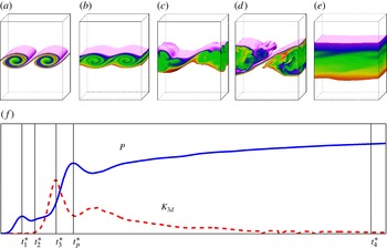
The life-cycle of a KH instability is divided into four phases, as suggested by Caulfield & Peltier (Reference Caulfield and Peltier2000). The end of each phase is marked by a transition time, to which we will refer as $t_{1}^{\ast }$ , $t_{2}^{\ast }$ , $t_{3}^{\ast }$ , $t_{4}^{\ast }$ hereafter, with $t^{\ast }=t{\rm\Delta}U/h_{0}$ being the non-dimensional time. The three-dimensional density structure of a simulation with $\mathit{Re}_{0}=900$ , simulation 7d in table 1, at these four transition stages is shown in figure 1.

Table 1.

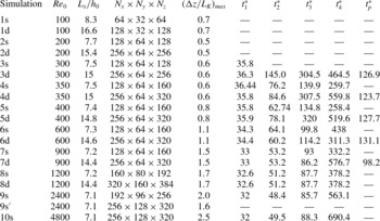
Description of the simulations carried out, and the transition times for each simulation. The letter next to each simulation number indicates if the simulation is single wavelength (s), or double wavelength (d). The superscript $\text{}^{\prime }$ indicates the mesh test simulation. $N_{x}$ , $N_{y}$ and $N_{z}$ are the number of grid points in the $x$ , $y$ and $z$ directions, respectively, for the velocity field. There are twice as many grid points in each direction for the density field. ${\rm\Delta}z$ represents the vertical grid spacing of the velocity field. In all simulations $J=0.03$ , $\mathit{Pr}=1$ . In single wavelength simulations $L_{z}=9h_{0}$ , and in double wavelength simulations $L_{z}=18h_{0}$ .

Figure 1.

The density structure of the KH billow at different stages at $t_{1}^{\ast }$ , $t_{2}^{\ast }$ , $t_{3}^{\ast }$ , $t_{p}^{\ast }$ and $t_{4}^{\ast }$ in (a–e) respectively for a $\mathit{Re}_{0}=900$ billow. These times correspond to the first maxima of the potential energy, the onset of three-dimensional instabilities, the maximum intensity of three-dimensional motions, the completion of pairing, and re-laminarization, respectively. The definition of the different stages is illustrated in (f) using the total potential energy, $P$ , and the three-dimensional turbulent kinetic energy, $K_{3d}$ .

The instability starts by re-distributing the vorticity of the initial vortex sheet and accumulating vorticity in the core of the billow (Corcos & Sherman Reference Corcos and Sherman1976). The core vortex of the billow drives the roll-up of the density interface as exhibited in figure 1(a). This process entrains fluids from both layers inside the core, while creating a strained interface on the braids connecting the cores. As a result the billow gains height and the potential energy of the flow increases. This phase ends at $t_{1}^{\ast }$ when the total potential energy of the billow, $P$ , reaches a maximum. We refer to this stage as the ‘saturation’ of the two-dimensional growth of the instability. The two-dimensional billow continues to evolve by exchanging energy with the mean flow and generating more mixed fluid inside the billow through molecular diffusion of the rolled interface. This phase ends with the onset of growth of three-dimensional secondary instabilities at $t_{2}^{\ast }$ . We define $t_{2}^{\ast }$ as the time when $K_{3d}/K_{0}$ first exceeds $10^{-3}$ , where $K_{3d}$ is the kinetic energy of the three-dimensional motions and $K_{0}$ the initial kinetic energy of the flow. As a result of the growth of the three-dimensional instabilities (studied in detail by Klaassen & Peltier Reference Klaassen and Peltier1985b ; Caulfield & Peltier Reference Caulfield and Peltier2000; Mashayek & Peltier Reference Mashayek and Peltier2012a ) small-scale chaotic motions develop in the flow field and more fluid from both layers is entrained inside the billow region. This state is referred to as the growing turbulence phase here. However, it should be noted that at low Reynolds numbers the flow lacks a wide spectrum of energy-containing to energy-dissipating length scales to exhibit developed turbulence. As the turbulent motions grow, they generate higher velocity gradients and therefore more viscous dissipation of the turbulent kinetic energy. After reaching a maximum intensity at the peak of $K_{3d}/K_{0}$ at $t_{3}^{\ast }$ , the decay of the three-dimensional motions starts. In this turbulence decaying phase, the mixing of the density field continues and a re-laminarized stable flow state is reached at the end of the life-cycle, $t_{4}^{\ast }$ . At this time the turbulent motions are very small. We define $t_{4}^{\ast }$ as the time when $K_{3d}/K_{0}$ drops below  $10^{-3}$ .

When vortex pairing is allowed, the evolution of the billow depends on the phase in which pairing is complete. The completion of vortex pairing is defined as the time at which the potential energy, $P$ , reaches its second peak, at $t_{p}^{\ast }$ , when the two vortices have wrapped around each other and the resulting paired billow reaches a maximum height. In figure 1, $t_{p}^{\ast }$ occurs in the turbulence decay phase at $\mathit{Re}_{0}=900$ . Therefore, the billows have gone through a full transition to turbulence before pairing. This sequence significantly suppresses pairing. However, as will be seen in subsequent sections, at lower Reynolds numbers, e.g. at $\mathit{Re}_{0}=400$ , the vortex pairing is complete in the early stages of turbulence growth, while significantly suppressing $K_{3d}$ , as also pointed out by Moser & Rogers (Reference Moser and Rogers1993). Therefore, at $t_{p}^{\ast }$ the billow is still fairly two-dimensional, and the pairing process is not disturbed by three-dimensional instabilities. In this case, the vertical extent of the paired billow is significantly larger than that of the primary billow, generating a high amount of stirring.

The values of the transition times are presented in table 1 for reference. This table indicates that the saturation time is close for all simulations, and close to the saturation time of 35 of Arratia, Caulfield & Chomaz (Reference Arratia, Caulfield and Chomaz2013). The other transition times are highly dependent on the Reynolds number and pairing process.

2.3. Energy partitions and transfer rates

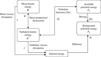
Quantitative description of the instability is assisted by an analysis of the exchange rates between different components of the energy budget. Based on earlier work of Lorenz (Reference Lorenz1955), Winters et al. (Reference Winters, Lombard, Riley and D’asaro1995) discuss a systematic description of the energetics in density-stratified flows for a closed system, which will be followed here. Another description of energy transfer between energy partitions has been proposed by Tailleux (Reference Tailleux2013), suggesting a direct route to mixing through the energy transfer from the internal energy. However, for the objectives of the present study we found the description of the model of Winters et al. (Reference Winters, Lombard, Riley and D’asaro1995) sufficient. A schematic of energy partitions and the transfer rates between them are shown in figure 2. All the energy partitions are non-dimensionalized by dividing the dimensional energy partitions by ${\it\rho}_{0}({\rm\Delta}U)^{2}$ ; energy transfer rates are non-dimensionalized by dividing the dimensional energy transfer rates by ${\it\rho}_{0}({\rm\Delta}U)^{3}/h_{0}$ . The total volume-averaged non-dimensional kinetic energy, $K$ , is

(2.3) $$\begin{eqnarray}K=\frac{\langle \boldsymbol{u}\boldsymbol{\cdot }\boldsymbol{u}\rangle _{V}}{2({\rm\Delta}U)^{2}},\end{eqnarray}$$

where $u$ denotes the three-dimensional velocity field, and $\langle \;\rangle _{V}$ denotes an average over the domain volume.  Contributions to the total kinetic energy are usually partitioned to three components: the two-dimensional and the three-dimensional turbulent motions, and the mean flow. These are defined respectively as (Caulfield & Peltier Reference Caulfield and Peltier2000)

(2.4a−c ) $$\begin{eqnarray}K_{2d}=\frac{\langle \boldsymbol{u}_{2d}\boldsymbol{\cdot }\boldsymbol{u}_{2d}\rangle _{xz}}{2({\rm\Delta}U)^{2}},\quad K_{3d}=\frac{\langle \boldsymbol{u}_{3d}\boldsymbol{\cdot }\boldsymbol{u}_{3d}\rangle _{xyz}}{2({\rm\Delta}U)^{2}}\quad \text{and}\quad \overline{K}=\frac{\langle \overline{\boldsymbol{u}}\boldsymbol{\cdot }\overline{\boldsymbol{u}}\rangle _{z}}{2({\rm\Delta}U)^{2}},\end{eqnarray}$$

where

(2.5a−c ) $$\begin{eqnarray}\overline{\boldsymbol{u}}(z,t)=\langle \boldsymbol{u}\rangle _{xy},\quad \boldsymbol{u}_{2d}(x,z,t)=\langle \boldsymbol{u}-\overline{\boldsymbol{u}}\rangle _{y}\quad \text{and}\quad \boldsymbol{u}_{3d}(x,y,z,t)=\boldsymbol{u}-\overline{\boldsymbol{u}}-\boldsymbol{u}_{2d},\end{eqnarray}$$

and $\langle \;\rangle _{i}$ shows an average in the direction(s) $i$ . Then the turbulent kinetic energy is $K^{\prime }=K_{2d}+K_{3d}$ .

Figure 2.

A schematic of energy partitions and transfers between them based on the framework suggested by Winters et al. (Reference Winters, Lombard, Riley and D’asaro1995).

The total non-dimensional potential energy is defined as

(2.6) $$\begin{eqnarray}P=\frac{g\langle {\it\rho}z\rangle _{V}}{{\it\rho}_{0}({\rm\Delta}U)^{2}}.\end{eqnarray}$$

The background potential energy obtained through adiabatic rearrangement of fluid particles is

(2.7) $$\begin{eqnarray}P_{b}=\frac{g\langle {\it\rho}z_{\ast }\rangle _{V}}{{\it\rho}_{0}({\rm\Delta}U)^{2}},\end{eqnarray}$$

where $z_{\ast }$ is the new position of the fluid parcel located at $z$ in the adiabatically redistributed state with minimum potential energy. The new position $z^{\ast }$ is found by rearranging the fluid parcels (the fluid in each cell) into a statically stable profile, where density is a monotonically decreasing function of height, which varies between zero and $L_{z}$ (Caulfield & Peltier Reference Caulfield and Peltier2000). This arrangement gives a column of $N_{x}\times N_{y}\times N_{z}$ parcels that describe the background density profile ${\it\rho}(z^{\ast })$ . In a closed system the background potential energy can change only due to an irreversible mixing process, while the total potential energy, $P$ , alters due to the vertical displacement of heavy or light fluid parcels. The difference between the total potential energy, $P$ , and the background potential energy is defined as the available potential energy, $P_{a}$ . Then the non-dimensional available potential energy is

(2.8) $$\begin{eqnarray}P_{a}=P-P_{b}.\end{eqnarray}$$

The available potential energy represents the portion of the potential energy that can be exchanged with the kinetic energy reversibly.

The time rates of change of the different components of the energy budget provide a tool to investigate the evolution process. As shown in figure 2, through the shear production or destruction of turbulent kinetic energy, ${\it\Psi}$ , energy is extracted from or given back to the mean kinetic energy partition. Meanwhile the mean and turbulent kinetic energy irreversibly lose energy to the internal energy through the mean and turbulent viscous dissipation, $\overline{{\it\varepsilon}}$ and ${\it\varepsilon}^{\prime }$ . The total rate of dissipation of kinetic energy is then ${\it\varepsilon}=\overline{{\it\varepsilon}}+{\it\varepsilon}^{\prime }$ . The total, turbulent, and mean kinetic energy dissipation rates are defined as

(2.9a−c ) $$\begin{eqnarray}{\it\varepsilon}={\it\nu}\langle \mathsf{S}_{ij}\mathsf{S}_{ij}\rangle _{V},\quad \bar{{\it\varepsilon}}={\it\nu}\left\langle \left(\frac{\partial {\bar{u}}}{\partial z}\right)^{2}\right\rangle _{V},\quad {\it\varepsilon}^{\prime }={\it\varepsilon}-\bar{{\it\varepsilon}},\end{eqnarray}$$

where $\mathsf{S}_{ij}$ is the strain rate tensor, and ${\bar{u}}$ is the horizontally averaged $x$ component of velocity. The energy gained by $K^{\prime }$ through the shear production can be exchanged reversibly with the available potential energy through the turbulent buoyancy flux, ${\it\phi}_{b}^{\prime }$ . The buoyancy flux measures the rate of stirring. Because of the flow condition here, the mean kinetic energy cannot exchange energy with the available potential energy (i.e. the mean buoyancy flux is zero). Therefore, the total potential energy can only exchange energy with the turbulent kinetic energy and the internal energy. The latter occurs due to the molecular diffusion of the background density profile and at the rate ${\it\phi}_{i}$ . Mixing is an irreversible process through which the flow uses the available potential energy to increase the background potential energy at the rate ${\it\phi}_{M}$ . Therefore the rate of change of the background potential is $\text{d}P_{b}/\text{d}t^{\ast }={\it\phi}_{M}+{\it\phi}_{i}$ . The amount of mixing at any time, $M$ , is measured by the increase in the background potential energy from its initial state minus the diffusion that would occur if there were no mean flow, i.e.

(2.10) $$\begin{eqnarray}M=P_{b}-P_{b}(0)-{\it\phi}_{i}t^{\ast }=\int _{0}^{t^{\ast }}{\it\phi}_{M}(t)\text{d}t.\end{eqnarray}$$

The mixing efficiency is an important diagnostic for characterizing mixing. The instantaneous mixing efficiency is defined as the ratio of the energy consumed by the mixing process to the total energy extracted from the background shear layer, which is either spent on mixing or lost to the internal energy (Caulfield & Peltier Reference Caulfield and Peltier2000; Carpenter et al. Reference Carpenter, Lawrence and Smyth2007), i.e. 

(2.11) $$\begin{eqnarray}E_{i}=\frac{{\it\phi}_{M}}{{\it\phi}_{M}+{\it\varepsilon}}.\end{eqnarray}$$

Also, a commonly used measure of the efficiency of mixing is the instantaneous flux coefficient (Moum Reference Moum1996; Smyth et al. Reference Smyth, Moum and Caldwell2001; Carpenter et al. Reference Carpenter, Lawrence and Smyth2007; Smyth et al. Reference Smyth, Carpenter and Lawrence2007), defined as

(2.12) $$\begin{eqnarray}{\it\Gamma}_{i}=\frac{{\it\phi}_{M}}{{\it\varepsilon}^{\prime }},\end{eqnarray}$$

which is the ratio of the energy consumed by the mixing process to the energy lost to the internal energy through the action of turbulent motions.  In fully developed turbulent mixing caused by shear instabilities ${\it\Gamma}_{i}$ is close to 0.2 (Smyth et al. Reference Smyth, Moum and Caldwell2001; Carpenter et al. Reference Carpenter, Lawrence and Smyth2007; Smyth et al. Reference Smyth, Carpenter and Lawrence2007; Inoue & Smyth Reference Inoue and Smyth2009).

Also of interest are the cumulative measures of the efficiency of mixing as suggested by Caulfield & Peltier (Reference Caulfield and Peltier2000) and Peltier & Caulfield (Reference Peltier and Caulfield2003). These are defined as

(2.13) $$\begin{eqnarray}E_{c}=\int _{T}{\it\phi}_{M}\text{d}t^{\ast }/\!\left(\int _{T}{\it\phi}_{M}\text{d}t^{\ast }+\int _{T}{\it\varepsilon}\text{d}t^{\ast }\right),\end{eqnarray}$$

the cumulative mixing efficiency, and

(2.14) $$\begin{eqnarray}{\it\Gamma}_{c}=\int _{T}{\it\phi}_{M}\text{d}t^{\ast }/\!\int _{T}{\it\varepsilon}^{\prime }\text{d}t^{\ast },\end{eqnarray}$$

the cumulative flux coefficient, where $T$ is the duration of interest in the mixing event.

3. Numerical modelling

Using the Boussinesq approximation, a linear equation of state, and incompressible fluid assumption, the Navier–Stokes and continuity equations in a Cartesian coordinate system take the form

(3.1a,b ) $$\begin{eqnarray}\frac{\text{D}\boldsymbol{u}}{\text{D}t}=\frac{-\boldsymbol{{\rm\nabla}}p}{{\it\rho}_{0}}-\frac{{\it\rho}}{{\it\rho}_{0}}g\hat{\boldsymbol{k}}+{\it\nu}{\rm\nabla}^{2}\boldsymbol{u}\quad \text{and}\quad \boldsymbol{{\rm\nabla}}\boldsymbol{\cdot }\boldsymbol{u}=0,\end{eqnarray}$$

where $p$ denotes the pressure field, $\text{D}/\text{D}t$ denotes a material derivative and $\hat{\boldsymbol{k}}$ is the unit vertical vector. These equations, along with the advection–diffusion equation

(3.2) $$\begin{eqnarray}\frac{\text{D}{\it\rho}}{\text{D}t}={\it\kappa}{\rm\nabla}^{2}{\it\rho},\end{eqnarray}$$

are solved using a pseudo-spectral model described by Winters, MacKinnon & Mills (Reference Winters, MacKinnon and Mills2004) and modified by Smyth, Nash & Moum (Reference Smyth, Nash and Moum2005). This model uses a third-order Adams–Bashforth time advancement scheme.

Three-dimensional DNS of the full life-cycle of KH billows are performed at different initial Reynolds numbers, see table 1. These simulations are chosen to include a wide range of Reynolds numbers to cover the pre- and post-transition range. It should be noted that here we have followed the convention of using full scales to define the Reynolds number in (2.2), which gives Reynolds numbers four times greater than when half scales are used. When stated in terms of our definition of  $\mathit{Re}_{0}$ , our range of Reynolds numbers is comparable to previous numerical simulations of mixing in KH flows: $\mathit{Re}_{0}=1600$ in Cortesi et al. (Reference Cortesi, Smith, Yadigaroglu and Banerjee1999), $\mathit{Re}_{0}=2300$ in Caulfield & Peltier (Reference Caulfield and Peltier2000), $400<\mathit{Re}_{0}<1200$ in Smyth et al. (Reference Smyth, Nash and Moum2005), $\mathit{Re}_{0}=1200$ in Carpenter et al. (Reference Carpenter, Lawrence and Smyth2007), and $1200<\mathit{Re}_{0}<3200$ in Inoue & Smyth (Reference Inoue and Smyth2009).

In all simulations $J=0.03$ , $\mathit{Pr}=1$ , and $R=1$ . While values of $J$ in the open ocean are typically much greater than 0.03 (Peters, Gregg & Toole Reference Peters, Gregg and Toole1988; Forryan et al. Reference Forryan, Martin, Srokosz, Popova, Painter and Renner2013), values as low as 0.015 have been measured in the exchange flow through the Strait of Gibraltar (Wesson & Gregg Reference Wesson and Gregg1994). At $J=0.03$ the effect of stratification on the transition to turbulence is less significant compared to higher values of $J$ (Caulfield & Peltier Reference Caulfield and Peltier2000). Therefore, the transition to turbulence in our simulations is due to the same type of instabilities as in the homogeneous mixing layer experiments of Breidenthal (Reference Breidenthal1981) and Koochesfahani & Dimotakis (Reference Koochesfahani and Dimotakis1986). It should be noted that at high values of $J$ different types of secondary instabilities may develop (Mashayek et al. Reference Mashayek, Caulfield and Peltier2013), and make mixing qualitatively different from what we observe in the present paper. One and two wavelengths of the fastest growing instability, found from linear stability analysis, are simulated. For high Reynolds numbers only single wavelength simulations were performed due to our limitations in computational resources. The domain heights of $L_{z}=9h_{0}$ for single wavelength and $L_{z}=18h_{0}$ for double wavelength simulations are sufficiently high to ensure negligible vertical fluxes on top and bottom boundaries (Haigh Reference Haigh1995; Smyth et al. Reference Smyth, Moum and Caldwell2001; Inoue & Smyth Reference Inoue and Smyth2009). The spanwise length of the domain is $L_{y}=L_{x}/2$ , which almost accommodates at least one wavelength of the three-dimensional secondary instability (Arratia et al. Reference Arratia, Caulfield and Chomaz2013). According to the spanwise stability studies of Arratia et al. (Reference Arratia, Caulfield and Chomaz2013), the wavelength of spanwise instabilities, which originate on the braid for the low $J$ here, decreases with $\mathit{Re}_{0}$ , with its maximum being around $0.7L_{x}$ . All three-dimensional simulations were also performed in two dimensions by setting the spanwise domain length to zero.

The required resolution for the DNS of stratified flows with $\mathit{Pr}\leqslant 1$ is estimated from the Kolmogorov length scale,

(3.3) $$\begin{eqnarray}L_{K}=({\it\nu}^{3}/{\it\varepsilon})^{1/4}.\end{eqnarray}$$

In all our simulations the grid spacing of the velocity field (the coarse resolution) is smaller than $2.5L_{K}$ throughout the entire duration of the simulation, which satisfies the requirements suggested by Moin & Mahesh (Reference Moin and Mahesh1998) and Smyth & Winters (Reference Smyth and Winters2003). Also, a resolution sensitivity test was performed for simulation 9s ( $\mathit{Re}_{0}=2400$ ), as described by simulation $9\text{s}^{\prime }$ . Decreasing the spatial resolution by 33 % in simulation $9\text{s}^{\prime }$ resulted in a less than 4 % increase in the final amount of mixing. To check for aliasing errors due to the under-resolution of the fields, we have examined the energy spectra for high Reynolds number simulations. These spectra did not demonstrate an increase in energy for small scales, which is a sign of occurrence of aliasing errors, as pointed out by Winters et al. (Reference Winters, MacKinnon and Mills2004).

Periodic horizontal and free-slip vertical boundary conditions were applied. Basic velocity and density profiles in (2.1) are perturbed using the eigenfunctions from the numerical solution of the linear stability equation. The magnitude of this perturbation is large enough to cause a maximum displacement of $0.05h_{0}$ of the interface, and small enough for the perturbation to be linear. The amplitude of the two-dimensional perturbation had a negligible effect on mixing. Also, a random noise with the magnitude of $\pm 0.02{\rm\Delta}U$ is added to the velocity field, with its maximum being at the centre of the shear layer, to initiate three-dimensional and pairing secondary instabilities. Lowering the amplitude of the initial three-dimensional perturbation by a factor of 4, and the two-dimensional perturbations by a factor of 2 (two separate tests) resulted in small changes in mixing.

4. Overall amount of mixing

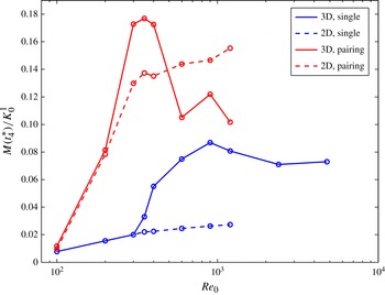
The variation in the total amount of mixing that the evolution of KH instability has produced until the re-laminarization stage at $t_{4}^{\ast }$ (note that this time is different for different $\mathit{Re}_{0}$ ) with the initial Reynolds number is presented in figure 3. This amount of mixing is normalized by $K_{0}^{1}$ , the initial kinetic energy of a shear flow in a $9h_{0}$ high domain; normalization by $K_{0}^{1}$ was necessary to make the comparison between different domain heights consistent.

Figure 3.

Variation of the amount of mixing gained at the end of the KH life-cycle normalized by the kinetic energy of a $9h_{0}$ high initial shear flow, i.e.  $M(t_{4}^{\ast })/K_{0}^{1}$ , with the Reynolds number for single three-dimensional billows (solid dark grey line, blue online), single two-dimensional billows (dashed dark grey line, blue online), double three-dimensional billows (solid light grey line, red online), and double two-dimensional billows (dashed light grey line, red online).

For a single KH billow, the total mixing shows an abrupt increase for $\mathit{Re}_{0}>300$ . The total background potential energy gained due to the mixing rises to 5.5 % of the initial kinetic energy at $\mathit{Re}_{0}=400$ from 2 % at $\mathit{Re}_{0}=300$ . This trend of increase in total mixing continues until a maximum mixing ratio of 8.7 % is reached at $\mathit{Re}_{0}=900$ . Similar to the laboratory mixing measurements of Breidenthal (Reference Breidenthal1981) and Koochesfahani & Dimotakis (Reference Koochesfahani and Dimotakis1986) the mixing trend here shows a transition that starts at $\mathit{Re}_{0}=300$ and completes at $\mathit{Re}_{0}=900$ . Before the start of the transition, i.e. for $\mathit{Re}_{0}\leqslant 300$ , the total two- and three-dimensional mixing are very close; the beginning of the transition is marked by the significant rise of the total mixing beyond the two-dimensional mixing. In the literature the mixing transition is commonly stated in terms of the outer-scale Reynolds number, $\mathit{Re}_{h}=h{\rm\Delta}U/{\it\nu}$ , where the outer scale, $h$ , describes the large scale of the flow. Following Smyth & Moum (Reference Smyth and Moum2000), we find the large scale $h$ and ${\it\delta}$ at any time from

(4.1a,b ) $$\begin{eqnarray}h(t)=\int _{L_{z}/2}^{L_{z}/2}\left(1-\left(\frac{2{\bar{u}}}{{\rm\Delta}U}\right)^{2}\right)\text{d}z\quad \text{and}\quad {\it\delta}(t)=\int _{L_{z}/2}^{L_{z}/2}\left(1-\left(\frac{2\bar{{\it\rho}}}{{\rm\Delta}{\it\rho}}\right)^{2}\right)\text{d}z,\end{eqnarray}$$

with ${\bar{u}}$ and $\bar{{\it\rho}}$ being averaged vertical velocity and density. Using this definition, in our single billow DNS, $h(t_{4}^{\ast })/h_{0}$ , which is the asymptotic outer scale of the flow at the end of the life-cycle, varies between 3 and 6, with the transition occurring between outer-scale Reynolds numbers of $900<\mathit{Re}_{h}<5000$ . This range is of the same order of magnitude as the transitional range of $10^{3}<\mathit{Re}_{h}<10^{4}$ , reported by Breidenthal (Reference Breidenthal1981) and Koochesfahani & Dimotakis (Reference Koochesfahani and Dimotakis1986). Beyond the Reynolds number of maximum mixing, our DNS exhibits a weaker dependence of mixing on $\mathit{Re}_{0}$ .

For double KH billows, the variation of mixing as a function of Reynolds number is strongly influenced by vortex pairing. At $\mathit{Re}_{0}=100$ , a Reynolds number too low to support three-dimensional or pairing instabilities, all two- and three-dimensional, single and double wavelength billows generate almost the same amount of mixing. At $\mathit{Re}_{0}=200$ , vortex pairing occurs, but the flow is still too diffusive for the three-dimensional instabilities to grow. Hence, there is a significant, and almost equal, increase in the amount of mixing for both two- and three-dimensional billows. At $\mathit{Re}_{0}=300$ , three-dimensional instabilities grow in addition to the vortex pairing becoming stronger (as seen from the two-dimensional double billow mixing trend). This further enhances the entrainment and mixing. A maximum mixing ratio of 17.6 % occurs at $\mathit{Re}_{0}=350$ . At $\mathit{Re}_{0}=400$ , the amount of mixing is still high. However, after this Reynolds number, while the two-dimensional double billows exhibit an increasing mixing trend, the three-dimensional double billows show a significant reduction in the amount of mixing. This is attributed to the earlier and more energetic growth of three-dimensional instabilities that suppress pairing. Interestingly, at these Reynolds numbers two-dimensional double KH billows generate more mixing than three-dimensional ones.

Unlike single KH billows, double billows do not manifest a clear mixing transition due to the intriguing effect of vortex pairing. The outer scale for these flows ranges between $6<h/h_{0}<8$ , and the outer-scale Reynolds number between $3000<\mathit{Re}_{h}<6500$ , within the transitional range observed by Breidenthal (Reference Breidenthal1981) and Koochesfahani & Dimotakis (Reference Koochesfahani and Dimotakis1986). However, the discrepancy between the experimental and DNS pairing billow mixing trends suggests that vortex pairing is not a common feature of laboratory KH billows generated using a splitter plate at low pre-transitional Reynolds numbers. This speculation is supported by flow visualizations of Konrad (Reference Konrad1976) and Breidenthal (Reference Breidenthal1981). At high Reynolds numbers, however, the trend of mixing in single and double DNS KH billows is similar (figure 3). In the rest of the paper, we investigate the flow properties to explain the trends in figure 3 in more detail.

5. Density structure of the billow

The effect of the Reynolds number on the density structure of the billow is significant through all the different phases of the evolution of the instability. Prior to the generation of three-dimensional instabilities at $t_{2}^{\ast }$ , a higher $\mathit{Re}_{0}$ produces a less diffuse density structure of the billow with sharper density gradients. Hence, at higher $\mathit{Re}_{0}$ the billow is more structured and the local baroclinic torques are stronger when the three-dimensional instabilities start to grow. The more significant effect of $\mathit{Re}_{0}$ is evident after the development of three-dimensional motions; the smaller scale vortices at higher $\mathit{Re}_{0}$ result in a more developed turbulence inside the billow where mixing is facilitated by smaller scale density gradients. 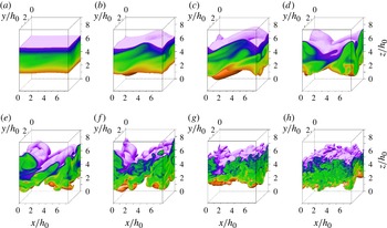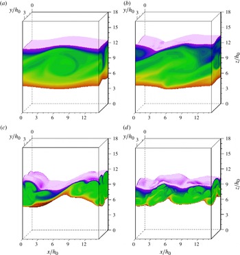As this effect is displayed well at $t_{3}^{\ast }$ , we show the density structure at this stage for increasing Reynolds numbers in figure 4, for single KH billows, and in figure 5, for double KH billows.

Figure 4.

Density field at $t_{3}^{\ast }$ , maximum intensity of turbulence, for single wavelength billows at $\mathit{Re}_{0}=$ (a) 300, (b) 350, (c) 400, (d) 600, (e) 900, ( f) 1200, (g) 2400, (h) 4800.

Figure 5.

Density field at $t_{3}^{\ast }$ , maximum intensity of turbulence, for double wavelength billows at $\mathit{Re}_{0}=$ (a) 300, (b) 400, (c) 900, and (d) 1200.

For single billows in figure 4, before the start of the mixing transition, i.e.  $\mathit{Re}_{0}<300$ the flow is not energetic enough to overcome viscous effects and sustain three-dimensional instabilities. Klaassen & Peltier (Reference Klaassen and Peltier1985b ) suggest that there is a critical Reynolds number below which secondary instabilities do not form, and this critical Reynolds number depends on $J$ and $\mathit{Pr}$ . In our DNS, for $\mathit{Re}_{0}>300$ the three-dimensionality starts by a combination of streamwise vortices on the braid and convective instabilities on the edges of the billow. This type of secondary instability is expected as the bulk Richardson number, $J$ , is small (Caulfield & Peltier Reference Caulfield and Peltier2000; Arratia et al. Reference Arratia, Caulfield and Chomaz2013). At the stage shown in figure 4 the three-dimensional instabilities have led the flow to a state of chaotic small-scale motions. In the process of the transition, e.g. at $\mathit{Re}_{0}=400$ and $\mathit{Re}_{0}=600$ , the three-dimensionality of the density structure is strong, yet length scales of variations in the spanwise direction are very limited. The stirring in these cases is governed by the large-scale eddy that still carries the structure of the initial streamwise vortices. At $\mathit{Re}_{0}=900$ , a range of different scale vortices are generated, indicating more developed turbulence. Some residues of the initial three-dimensional instabilities that triggered the turbulence are still preserved. Through the action of the larger vortices unmixed fluid is entrained inside the turbulent billow region. At high $\mathit{Re}_{0}$ , e.g. $\mathit{Re}_{0}=4800$ , the two-dimensional structure of the billow is mainly destroyed, and the density field exhibits small-scale motions developed throughout the turbulent region. This is similar to the homogenization of the density and vorticity fields inside the turbulent region of the billow after the development of three-dimensional instabilities at high Reynolds numbers simulated by Mashayek & Peltier (Reference Mashayek and Peltier2013).

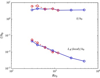
As large-scale eddies are mainly responsible for the stirring, and small-scale eddies for the mixing mechanism, we examine ${\it\delta}$ and local $L_{K}$ (the minimum Kolmogorov scale in the turbulent region) at $t=t_{3}^{\ast }$ , in figure 6. This figure shows that at $t_{3}^{\ast }$ , ${\it\delta}$ attains slightly higher values through the mixing transition up to $\mathit{Re}_{0}=900$ . For higher Reynolds numbers ${\it\delta}$ at maximum intensity of turbulence first decreases, implying suppression of the large-scale motions, and then reaches a constant for $\mathit{Re}_{0}>1200$ . We associate this reduction in the average density thickness, and therefore vertical stirring, with a comprehensive development of small-scale eddies in the billow that destroys the large-scale structure of the billow. Also, we speculate that due to the disappearance of large density gradients the local energizing effect of the baroclinic torques (Cortesi et al. Reference Cortesi, Smith, Yadigaroglu and Banerjee1999; Staquet Reference Staquet2000), where the Richardson number is locally higher than its bulk value, on three-dimensional motions weakens. Hence, the strength of large-scale two- and three-dimensional structures is suppressed by full development of small-scale motions at high $\mathit{Re}_{0}$ .

Figure 6.

Reynolds number dependence of the large scale, ${\it\delta}/h_{0}$ (top lines), and small scale local Kolmogorov length scale, $L_{K}(local)/h_{0}$ (bottom lines), at $t_{3}^{\ast }$ . The solid lines indicate single billows, and the dashed lines double billows.

The smallest scale of motion is estimated by the Kolmogorov scale, defined by (3.3), and can be related to the Reynolds number by $L_{K}\cong C_{K}{\it\delta}_{0}\mathit{Re}^{-3/4}$ , with $C_{k}$ being a constant (Tennekes & Lumley Reference Tennekes and Lumley1972). Therefore, the smallest scale at $\mathit{Re}_{0}=2400$ should be approximately 3.8 times smaller than that at $\mathit{Re}_{0}=400$ . This ratio is 6.2 from figure 6, since local minimum Kolmogorov length scales are shown here, rather than the volume-averaged values. Figure 6 suggests that the ratio of large to small scales of the density field grows as $\mathit{Re}_{0}$ increases (e.g. this ratio increases from ${\sim}65$ to ${\sim}1300$ as $\mathit{Re}_{0}$ increases from 400 to 2400). However, the large scale varies less significantly with $\mathit{Re}_{0}$ , and becomes independent of $\mathit{Re}_{0}$ for sufficiently high Reynolds numbers. The development of small scales enhances mixing initially as $\mathit{Re}_{0}$ increases. However, further lowering of small scales, without increasing the size of large scales, does not increase mixing at high $\mathit{Re}_{0}$ . These two states of mixing at low and high $\mathit{Re}_{0}$ have been described as ‘diffusion-limited’ and ‘entrainment-limited’ mixing by Broadwell (discussed by Breidenthal Reference Breidenthal1981), respectively.

Figure 7.

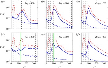
Time evolution of the volume-averaged rate of dissipation of the scalar, ${\it\chi}$ (light grey dashed line, red online), and the volume-averaged rate of dissipation of kinetic energy, ${\it\varepsilon}$ (dark grey solid line, blue online), and the volume-averaged rate of dissipation of mean kinetic energy, $\bar{{\it\varepsilon}}$ (dark grey dashed line, blue online), for different Reynolds numbers. (a–c) Single billows, (d–f) double billows. The dashed black vertical times show the transition times: $t_{1}^{\ast }$ , $t_{2}^{\ast }$ , $t_{3}^{\ast }$ , $t_{4}^{\ast }$ ( $t_{4}^{\ast }$ is off the time axis in some cases), and the grey solid vertical line (green online) in (d) and (e) shows the time of completion of pairing: $t_{p}^{\ast }$ .

For double billows in figure 5, the size of the large-scale eddy is primarily set by the pairing process. At $\mathit{Re}_{0}=300$ and 400, the large-scale eddy, ensuing from the vortex pairing, dominates the flow, with some weak three-dimensional structures present. At $\mathit{Re}_{0}=900$ , the size of the large-scale eddy is significantly diminished, as the vortex-pairing-induced entrainment is lost. While three-dimensional motions are strong for this case, they do not compensate for the effect of suppressed pairing, and ${\it\delta}$ decreases significantly at $\mathit{Re}_{0}=900$ , see figure 6. At $\mathit{Re}_{0}=1200$ , the size of the large-scale structure of the billow is even more diminished as smaller scale structures develop inside the billow. Three-dimensional motions in billows with vortex pairing, at their maximum intensity, are significantly suppressed compared to the same Reynolds number billows without pairing. This is because a significant portion of the energy extracted from the background shear flow is consumed by pairing, and is converted to the potential energy, or two-dimensional kinetic energy form rather than three-dimensional kinetic energy. Hence, turbulence is more limited for paired billows and the small scale, $L_{K}$ , does not drop down to the minimum reached in single billows.

6. Kinematics of mixing

To gain more insight into the properties of mixing observed in figures 4 and 5 we examine the structure of density and velocity fields in this section. Figure 7 presents the time evolution of the volume-averaged rate of dissipation of the kinetic energy, ${\it\varepsilon}=\bar{{\it\varepsilon}}+{\it\varepsilon}^{\prime }$ , and the volume-averaged rate of dissipation of the scalar field, defined as

(6.1) $$\begin{eqnarray}{\it\chi}=2{\it\kappa}\boldsymbol{{\rm\nabla}}{\it\rho}\boldsymbol{\cdot }\boldsymbol{{\rm\nabla}}{\it\rho}.\end{eqnarray}$$

The former is a measure of the action of the local strain rates on the generation of small-scale structures in the flow, and the latter is a measure of the scalar diffusion across the scalar interfaces, which have enhanced interfacial area and scalar gradient through the formation of small-scale motions.

The first peak in ${\it\chi}$ , associated with the two-dimensional roll-up of the billow, has the same maximum value for all Reynolds numbers. The second peak in ${\it\chi}$ , related to the increase in ${\it\varepsilon}$ , however, shows a Reynolds number dependence. For a single billow, the turbulent density field is more dissipative at $\mathit{Re}_{0}=900$ compared to $\mathit{Re}_{0}=400$ . However, at $\mathit{Re}_{0}=1200$ the density field become slightly less dissipative in the turbulent phase, indicating that a limit in the increase of interfacial area and density gradients has been reached. The dissipation of the total kinetic energy, however, increases monotonically with $\mathit{Re}_{0}$ as local strain rates become larger at higher $\mathit{Re}_{0}$ . For double billows, the second peak in ${\it\chi}$ is due to the two-dimensional pairing process. The dissipation of the scalar field caused by the development of small scales diminishes at $\mathit{Re}_{0}=1200$ compared to that at $\mathit{Re}_{0}=900$ , while the dissipation of kinetic energy increases with $\mathit{Re}_{0}$ . Figure 7 also indicates that the during the turbulent phase the turbulent rate of dissipation of kinetic energy, ${\it\varepsilon}^{\prime }$ , can reach one to two orders of magnitude higher than the mean rate of dissipation of kinetic energy, $\bar{{\it\varepsilon}}$ . This suggests that the assumption of Osborn (Reference Osborn1980) that the mean rate of dissipation of kinetic energy is negligible might be a good approximation at the turbulent phase, even at our low Reynolds numbers.

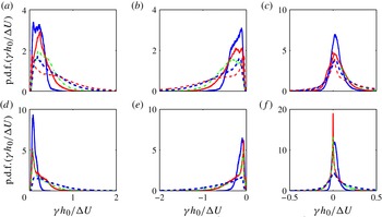
The probability density functions of the local principal strain rates at $t_{3}^{\ast }$ , presented in figure 8, show the kinematics of small scales in the density fields shown in figures 4 and 5. These probability density functions are found from the normalized number of occurrences of local values of strain rate within a sufficiently small window of strain rates. The principal strain rates ${\it\gamma}_{1}$ , ${\it\gamma}_{2}$ and ${\it\gamma}_{3}$ , shown in figure 8 are the eigenvalues of the local strain rate tensor, with ${\it\gamma}_{1}$ being the expansive strain rate (always positive), ${\it\gamma}_{2}$ the compressive strain rate (always negative), and ${\it\gamma}_{3}$ a strain rate of indeterminate sign, so that ${\it\gamma}_{1}+{\it\gamma}_{2}+{\it\gamma}_{3}=0$ . The fact that ${\it\gamma}_{3}$ is biased towards positive values for all flows points out that the flow tends to form sheets of small-scale structures rather than filaments (Smyth Reference Smyth1999), even at high $\mathit{Re}_{0}$ . As $\mathit{Re}_{0}$ increases, the range of strain rates extends to high strain rates, e.g.  ${\it\gamma}^{\ast }={\it\gamma}h_{0}/{\rm\Delta}U>1$ . This is line with the Kolmogorov scaling of ${\it\gamma}^{\ast }\sim \mathit{Re}_{0}^{1/2}$ . However, for single billows this extension to higher strain rates is at the cost of less occurrence of intermediate strain rates, e.g. $0.1<{\it\gamma}^{\ast }={\it\gamma}h_{0}/{\rm\Delta}U<0.5$ , which are the most prevalent at low Reynolds numbers. Especially, at $\mathit{Re}_{0}=2400$ , there is a significant drop in the probability of occurrence of these intermediate strain rates. This indicates that the flow structures that cause mid-range strain rates at lower Reynolds numbers have disappeared at $\mathit{Re}_{0}=2400$ . Also, there is a bias towards the occurrence of small strain rates, i.e. ${\it\gamma}^{\ast }<0.2$ , at $\mathit{Re}_{0}=2400$ . This can be associated with the shrinkage of the billow size, and development of small scales at the edge of the turbulent region, with low local velocity gradients. For billows with pairing, high and intermediate strain rates are significantly suppressed, except for $\mathit{Re}_{0}=1200$ .

Figure 8.

Probability density functions of the principal strain rates at $t_{3}^{\ast }$ for (a,d) ${\it\gamma}_{1}$ , (b,e) ${\it\gamma}_{2}$ , and (c,f) ${\it\gamma}_{3}$ , for a single billow (a–c), and double billows (d–f). Different line styles indicate different Reynolds numbers: solid dark grey (blue online), $\mathit{Re}_{0}=400$ ; solid light grey (red online), $\mathit{Re}_{0}=600$ ; dashed-dotted light grey (green online), $\mathit{Re}_{0}=900$ ; dashed dark grey (blue online), $\mathit{Re}_{0}=1200$ ; and dashed light grey (red online), $\mathit{Re}_{0}=2400$ .

Dissipation of the density field occurs over the interface of the sheets caused by the expansive strain rates; the thickness of the interface scales with $({\it\kappa}/{\it\gamma})^{1/2}$ . To measure the dissipation at different scales, we define the scalar dissipation spectra by applying a Fourier transform to the scalar field in the streamwise direction at each $(y,z)$ point and then averaging over the middle section of the domain, $L_{z}/2-9h_{0}/8<z<L_{z}/2+9h_{0}/8$ , and also in the spanwise direction. In terms of the streamwise wavenumber, $k$ , this scalar spectrum is

(6.2a,b ) $$\begin{eqnarray}{\it\psi}(k_{i})=(\hat{{\it\rho}})^{2},\quad \frac{2{\rm\pi}}{L_{x}}\mathop{\sum }\limits_{i=1}^{N_{x}/2}{\it\psi}(k_{i})=\langle {\it\rho}^{2}\rangle _{xyz},\end{eqnarray}$$

with $\hat{\ }$ denoting the Fourier transform. The dissipation rate spectrum is then

(6.3) $$\begin{eqnarray}{\it\chi}_{i}=4{\rm\pi}{\it\kappa}k_{i}^{2}{\it\psi}(k_{i}).\end{eqnarray}$$

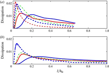
The scalar dissipation spectra of the billows at $t_{3}^{\ast }$ are shown in figure 9. These spectra have been normalized so that the area below each curve gives the total scalar dissipation. As already seen in figure 7, for single billows the maximum scalar dissipation occurs at $\mathit{Re}_{0}=900$ , where the peaks of ${\it\varepsilon}$ and ${\it\chi}$ are almost simultaneous. The trends of the scalar dissipation in figures 7 and 9 show the correlation between ${\it\chi}$ and mixing. The amount of dissipation at each length scale measures the magnitude of density gradients and available interfacial area at that scale. For increasing $\mathit{Re}_{0}$ , the length scale of maximum scalar dissipation shifts from large scales to smaller scales. The distribution of scalar dissipation also significantly changes for increasing $\mathit{Re}_{0}$ : the scalar dissipation largely occurs around the small dissipative scales rather than at a wide range of scales. At $\mathit{Re}_{0}=1200$ , there is a significant reduction in the amount of dissipation for $l/h_{0}>0.2$ . This is another indication of the destruction of large- and intermediate-scale motions at high Reynolds numbers. Thus, as $\mathit{Re}_{0}$ increases, while the rate of dissipation at dissipative small length scales increases, the total dissipation saturates to a limit set by the available interfacial area and density gradients.

Figure 9.

Scalar dissipation at different length scales at $t_{3}^{\ast }$ for different $\mathit{Re}_{0}$ for (a) single billows, and (b) double billows. See caption of figure 8 for the colour coding.

For double billows, scalar dissipation is evenly distributed between scales from the dissipative range to double billow wavelength. This is because small-scale motions are still under-developed in these flows. At $\mathit{Re}_{0}=1200$ , where the small diffusive and dissipative scales have developed simultaneously (figure 7), the single and double billows exhibit more similar scalar dissipation spectra.

7. Energy partitions

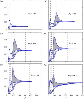
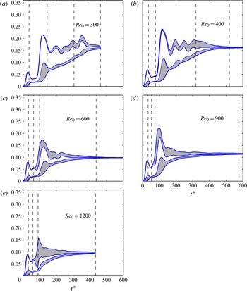
In this section we discuss the evolution of the energy partitions through different phases of the lifetime of the billow. Figure 10 shows the time variation of the background and available potential energy, and two- and three-dimensional turbulent kinetic energy partitions added together in turn, for a single wavelength billow. Figure 11 shows the energy partitions presented in the same fashion as in figure 10 for double wavelength billows. In these figures the gain in the background potential energy due to the diffusion because of the background density difference, i.e. ${\it\phi}_{i}t^{\ast }$ , is excluded. The summation of these four energy partitions shows the total amount of energy that is extracted by the instability from the background flow and not lost to the internal energy through the viscous dissipation. The summation of the background and available potential energy partitions indicates the portion of this extracted energy that is given to the total potential energy through the turbulent buoyancy flux.

Figure 10.

Time evolution of the energy partitions normalized by $K_{0}^{1}$ for single wavelength billows. The bottom line shows the background potential energy partition: $P_{b}-P_{b}(0)-{\it\phi}_{i}t^{\ast }$ . The second line from the bottom adds the available potential energy partition, $P_{a}-P_{a}(0)$ , to the first line, giving the total potential energy partition, $P-P(0)-{\it\phi}_{i}t^{\ast }$ . The third line is the addition of the two-dimensional turbulent kinetic energy, $K_{2d}$ , to the total potential energy. The fourth line adds the three-dimensional turbulent kinetic energy partition, $K_{3d}$ , to the summation of these three partitions, giving the total energy extracted by the instability from the background shear layer. $P_{a}$ and $K_{3d}$ partitions are shaded. The vertical lines show the transition times.

Figure 11.

Time evolution of the energy partitions normalized by $K_{0}^{1}$ for double wavelength billows. The energy partitions have been added together as explained in the caption of figure 10.

8. Rate of mixing

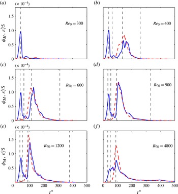
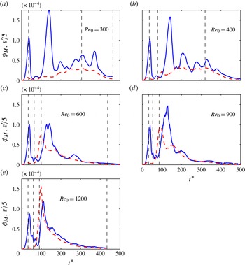
In this section we focus on the rate of mixing, ${\it\phi}_{M}$ . To investigate the efficiency of the mixing process, based on the flux coefficient definition, ${\it\Gamma}_{i}$ , we also study the turbulent viscous dissipation rate, ${\it\varepsilon}^{\prime }$ (see figure 2). Figure 12 shows the time evolution of these two rates for single billows, and figure 13 for double billows.

Figure 12.

Time evolution of the rate of mixing (solid line) and turbulent viscous dissipation rate divided by 5 (dashed line) for single wavelength billows for increasing Reynolds numbers. The vertical lines show the transition times.

Figure 13.

Time evolution of the rate of mixing (solid line) and turbulent viscous dissipation rate divided by 5 (dashed line) for double wavelength billows for increasing Reynolds numbers. The vertical lines show the transition times.

8.1. Single wavelength billows

In single KH billows, the entire mixing event consists of two major parts, each having a peak in the rate of mixing. The first peak corresponds to the two-dimensional roll-up of the primary instability and occurs at or after saturation, depending on $\mathit{Re}_{0}$ . The second peak occurs either at or slightly after $t_{3}^{\ast }$ . The pre-transition flow at $\mathit{Re}_{0}\leqslant 300$ lacks the second peak as no significant three-dimensionality is generated. As $\mathit{Re}_{0}$ increases the two peaks of the mixing rate gradually move closer together. This is because for higher $\mathit{Re}_{0}$ the mixing due to the roll-up is delayed more, and also the three-dimensional motions grow earlier. At $\mathit{Re}_{0}=4800$ the two peaks in mixing have become so close that there is almost no distinction between the two-dimensional mixing caused by the roll-up and the three-dimensional mixing caused by the growth of secondary instabilities.

As already seen in figure 10, a significant portion of the mixing takes place in phase 4 for all $\mathit{Re}_{0}>300$ . The occurrence of the highest ${\it\phi}_{M}$ at or slightly after $t_{3}^{\ast }$ indicates that the stretching of the density field by three-dimensional motions is an important mechanism in providing the interfacial area between the scalars to enhance the rate of mixing. For some $\mathit{Re}_{0}$ the maximum ${\it\phi}_{M}$ occurs slightly after $t_{3}^{\ast }$ . This suggests that, although the small-scale motions have started to decay, their interaction with each other and action on stretching of the density field is still strong enough to enhance the rate of mixing. Also, there is a delay in the response of the diffusion of the density field at small scales to the maximum stretching of the density field at the highest strain rates. This delay time has been modelled by Barenblatt et al. (Reference Barenblatt, Bertsch, Passo, Prostokishin and Uchi1993) as the delay time of the turbulence in diffusing a temperature gradient. By assuming that the velocity fluctuations caused by the tangential stresses in their model scale with $({\it\gamma}{\it\nu})^{1/2}$ , we obtain their modelled delay time in a dimensionless form as

(8.1) $$\begin{eqnarray}{\it\tau}^{\ast }=l_{t}^{\ast }{\it\gamma}_{t}^{\ast }\mathit{Re}_{0}^{1/2},\end{eqnarray}$$

where $l_{t}^{\ast }$ and ${\it\gamma}_{t}^{\ast }$ are dimensionless characteristic average length and strain rate scales of turbulence. By assuming a Taylor scaling for these scales, and ${\it\gamma}_{t}^{\ast }\sim 0.2$ for the Taylor scale strain rates, see Rahmani, Seymour & Lawrence (Reference Rahmani, Seymour and Lawrence2014), we get ${\it\tau}^{\ast }\sim 2$ . The time lag is clearly larger for lower Reynolds numbers as the average length scales are larger due to the under-development of turbulence.

Through the mixing transition, higher maximum mixing rates are generated for higher $\mathit{Re}_{0}$ , with the highest rate of mixing and dissipation of kinetic energy at $\mathit{Re}_{0}=1200$ . While the mixing rates near $t_{3}^{\ast }$ drop considerably for $\mathit{Re}_{0}=4800$ , the turbulence remains almost as dissipative as that at $\mathit{Re}_{0}=900$ . This is an indication of a reduction in efficiency of mixing due to the limitations in entrainment: small-scale motions cause high dissipation rates while the rate of mixing is suppressed by the reduced extent of large-scale motions.

The turbulent kinetic energy dissipation rate follows the trend of the mixing rate in the three-dimensional phases. The ${\it\varepsilon}^{\prime }/5$ and ${\it\phi}_{M}$ curves become very close shortly after $t_{3}^{\ast }$ . This match, intentionally assisted by dividing ${\it\varepsilon}^{\prime }$ by 5, suggests a universal value of 0.2 for ${\it\Gamma}_{i}$ observed in previous studies near the end of the KH life-cycle (Smyth et al. Reference Smyth, Moum and Caldwell2001, Reference Smyth, Carpenter and Lawrence2007; Inoue & Smyth Reference Inoue and Smyth2009).

9. Mixing efficiency

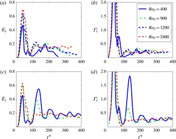
The instantaneous mixing efficiency and flux coefficient for different Reynolds numbers, defined by (2.11) and (2.12), are presented in figure 14. The pre-turbulent $E_{i}$ increases with $\mathit{Re}_{0}$ , and spikes at 0.7 for $\mathit{Re}_{0}=2400$ . This value is close to the instantaneous mixing efficiencies obtained by Caulfield & Peltier (Reference Caulfield and Peltier2000), Staquet (Reference Staquet2000) and Mashayek & Peltier (Reference Mashayek and Peltier2013) in the pre-turbulent stages. The pre-turbulent flux coefficients, however, reach high values of ${\sim}6$ (not shown in the figure), as ${\it\varepsilon}^{\prime }$ is negligible in this phase. During the turbulent phase, for single billows, $E_{i}$ fluctuates around ${\sim}0.15$ , and ${\it\Gamma}_{i}$ around ${\sim}0.2$ . As turbulence decays, $E_{i}$ drops for most $\mathit{Re}_{0}$ , but ${\it\Gamma}_{i}$ remains constant. The turbulent mixing efficiencies observed here are slightly lower than those obtained by Staquet (Reference Staquet2000) and Mashayek & Peltier (Reference Mashayek and Peltier2013) for higher $J$ , but are in the range of turbulent mixing efficiencies computed by Caulfield & Peltier (Reference Caulfield and Peltier2000) for similar $J$ . Our turbulent ${\it\Gamma}_{i}$ of ${\sim}0.2$ agrees with the DNS and field observations of Smyth et al. (Reference Smyth, Moum and Caldwell2001), and DNS of Carpenter et al. (Reference Carpenter, Lawrence and Smyth2007) and Smyth et al. (Reference Smyth, Carpenter and Lawrence2007). For billows with pairing, the high-efficiency pre-turbulent stage is longer. This stage is followed by a turbulent phase, in which $E_{i}$ and ${\it\Gamma}_{i}$ both drop to mean values that are higher than their counterpart single billow mean values. This is because for paired billows, even in the turbulent phase, the two-dimensional process of stirring and mixing still plays an important role so that it induces high-efficiency mixing.

Figure 14.

Time evolution of the instantaneous mixing efficiency, $E_{i}$ , and the instantaneous flux coefficient, ${\it\Gamma}_{i}$ for different Reynolds numbers for single billows (a,b), and double billows (c,d).

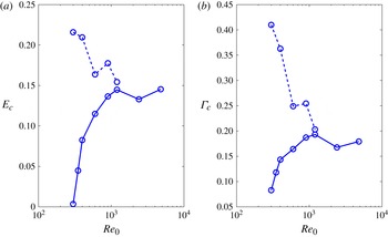
Figure 14 suggests that $E_{i}$ and ${\it\Gamma}_{i}$ are both useful measures of the mixing efficiency through different stages of the flow. For transitional Reynolds numbers, in the turbulent phase, $E_{i}$ and ${\it\Gamma}_{i}$ both increase as $\mathit{Re}_{0}$ increases, e.g. compare $\mathit{Re}_{0}=400$ and 900 for single billows in figure 14. However, for $\mathit{Re}_{0}=2400$ , the efficiency decreases during the turbulent phase. The cumulative mixing efficiencies in figure 15 present the total efficiency of the mixing event during the turbulent stage, from $t_{2}^{\ast }$ to $t_{4}^{\ast }$ , as defined in (2.13) and (2.14), for increasing $\mathit{Re}_{0}$ . The cumulative mixing efficiency and flux coefficient significantly increase with increasing $\mathit{Re}_{0}$ through the mixing transition for single billows. For higher Reynolds numbers, $E_{c}$ and ${\it\Gamma}_{c}$ are less $\mathit{Re}_{0}$ dependent. The highest ${\it\Gamma}_{c}$ of 0.14 for single billows is close to the cumulative turbulent mixing efficiency of ${\sim}0.14$ in simulations of Peltier & Caulfield (Reference Peltier and Caulfield2003), and lower than the overall cumulative mixing efficiency of ${\sim}0.2$ found by Caulfield & Peltier (Reference Caulfield and Peltier2000), both for a close value of $J$ . The non-monotonic variation of the mixing efficiency with $\mathit{Re}_{0}$ is similar to the non-monotonic change of the vertical mass fluxes with stratification in studies by Phillips (Reference Phillips1972), Posmentier (Reference Posmentier1977) and Linden (Reference Linden1979) for stably stratified turbulent shear flows. In these studies the formation of microstructures within a stable density stratification created local mixing and step functions in the density profile that enhanced the buoyancy fluxes after they have been suppressed by the strong stratification. Here, we also observe how small-scale motions can raise the mixing efficiency after the destruction of large-scale turbulent motions.

Figure 15.

Variation of the cumulative mixing efficiency (between $t_{2}^{\ast }$ and $t_{4}^{\ast }$ ),  $E_{c}$ , and the cumulative flux coefficient (between $t_{2}^{\ast }$ and $t_{4}^{\ast }$ ),  ${\it\Gamma}_{c}$ with the Reynolds number. The solid line indicates single billows, and the dashed line double billows.

Low Reynolds number billows with pairing exhibit much higher overall mixing efficiencies as the mixing process is essentially laminar. But paired and single billows demonstrate similar ${\it\Gamma}_{c}$ and $E_{c}$ for $\mathit{Re}_{0}=1200$ , where pairing is severely suppressed by three-dimensional motions. The trends of variation of the cumulative mixing efficiency and flux coefficient with $\mathit{Re}_{0}$ suggest that there is a correlation between $E_{c}$ (or ${\it\Gamma}_{c}$ ) and the overall mixing as presented in figure 3.