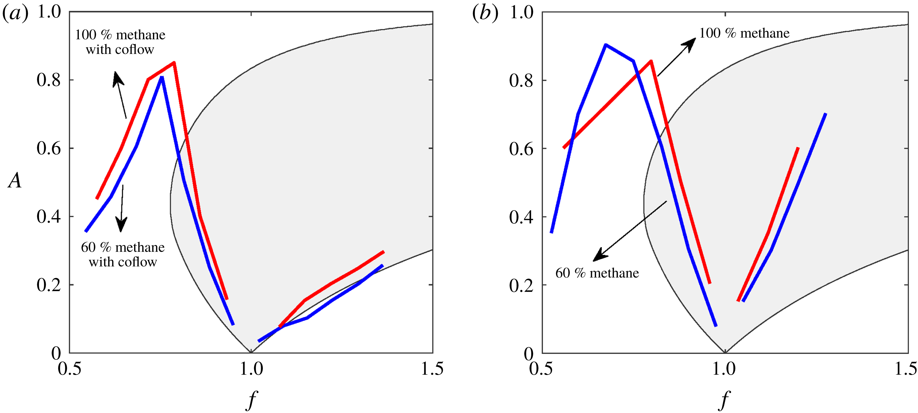
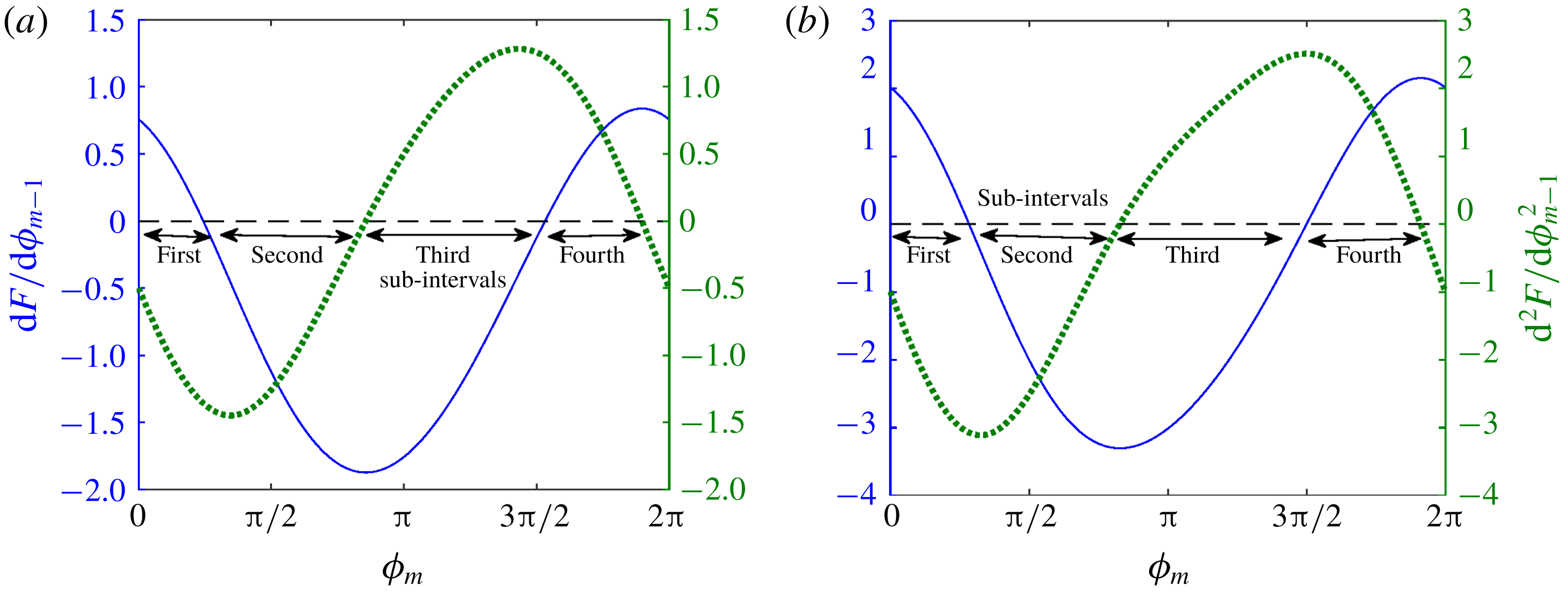
1 Introduction
A combustor is a system designed to hold a flame in a confined environment, through which fuel–air mixture is burnt. In such systems, there is an interaction between heat release rate of the flame and acoustic field of the combustor. This interaction may lead to detrimental high-amplitude pressure fluctuations, termed combustion instability. Acoustic field perturbs the flame, generating an unsteady heat release rate, which is a strong source of sound. Acoustic waves thus generated in turn affect the flame, forming a feedback loop. This loop supplies acoustic energy in the combustor when unsteady heat release and acoustic pressure oscillations are in phase (Rayleigh Reference Rayleigh1878). If the energy supply overcomes the damping present in the system, then self-sustained combustion instability occurs.
The mechanism through which acoustic fluctuations perturb the flame depends on the configuration of the burner and characteristics of the flame. A variety of burner configurations are available to anchor the flame. Anchoring through a bluff body is one such configuration used in a number of engines such as jet afterburners and ramjets (Huang & Yang Reference Huang and Yang2009). In this configuration, a bluff body is placed across the flow field creating a low-velocity zone, where flame anchors. The presence of the bluff body causes a recirculation zone behind it, which becomes hydrodynamically unstable and sheds vortices for the flow conditions encountered in the combustor.
During combustion, hot products form the major part of the recirculation zone, while the cold unburnt reactants flow along the outer edge of the bluff body. The shed vortices engulf both the products and reactants but do not allow them to come in contact due to the strong shear present in the vortices (Schadow & Gutmark Reference Schadow and Gutmark1992). As the vortices diffuse, the cold reactants are ignited by the contact with the hot products, which lead to sudden combustion and therefore unsteady heat release rate (Kaskan & Noreen Reference Kaskan and Noreen1955; Rogers & Marble Reference Rogers and Marble1956; Zukoski & Marble Reference Zukoski and Marble1956). Acoustic waves are then generated, which affects the vortex shedding process (Smith Reference Smith1985; Smith & Zukoski Reference Smith and Zukoski1985; Matveev & Culick Reference Matveev and Culick2003), which in turn produces further waves, closing the feedback loop. The above vortex-driven combustion instability also occurs when the vortex breaks down on interaction with an obstacle, releasing energy which feeds the acoustic field (Smith & Zukoski Reference Smith and Zukoski1985; Ken, Trouve & Daily Reference Ken, Trouve and Daily1991).
In previous experimental investigations (Poinsot et al. Reference Poinsot, Trouve, Veynante, Candel and Esposito1987; Chakravarthy et al. Reference Chakravarthy, Shreenivasan, Boehm, Dreizler and Janicka2007), it was observed that during combustion instability, the frequency of vortex shedding synchronizes with the acoustic frequency of the combustor. This event of synchronization is termed lock-in. The above papers indicate that lock-in is accompanied by large-amplitude (detrimental) oscillations. However, recent investigations (Emerson & Lieuwen Reference Emerson and Lieuwen2015; Guan et al. Reference Guan, Gupta, Kashinath and Li2019) show that the response amplitude is lower during lock-in, which can be used as a strategy for open-loop control of thermoacoustic oscillations (Guan et al. Reference Guan, Gupta, Kashinath and Li2019). Therefore, at this point, it is unclear whether lock-in is detrimental or beneficial in combustion systems.
In the absence of an acoustic field, vortices are shed at the natural vortex shedding frequency, determined by the geometry of the burner and flow velocity. This can be represented as a self-sustained periodic oscillator. The acoustic field can be considered as an external agent forcing the above oscillator. This analogy is possible since the frequency of the acoustic field remains fairly unaltered during its interaction with the vortex shedding process (Poinsot et al. Reference Poinsot, Trouve, Veynante, Candel and Esposito1987; Chakravarthy et al. Reference Chakravarthy, Shreenivasan, Boehm, Dreizler and Janicka2007).
In the past, rigorous analysis has been performed both analytically and numerically on the behaviour of external forcing on self-sustained oscillators (Pikovsky, Rosenblum & Kurths Reference Pikovsky, Rosenblum and Kurths2003; Balanov et al.
Reference Balanov, Janson, Postnov and Sosnovtseva2008). The majority of lock-in investigations were performed on Van der Pol and Duffing types of oscillators. Their results suggest that the response of oscillators to external forcing can be complex such as quasi-periodic, periodic locked to the forcing frequency. Careful experimental investigations on self-excited jets (Li & Juniper Reference Li and Juniper2013a
) and flames (Li & Juniper Reference Li and Juniper2013b
,Reference Li and Juniper
c
) indicated the existence of the above-described features: quasi-periodicity and
 $1:1$
(frequency of the oscillator synchronizes with the forcing frequency) lock-in. They reported that
 $1:1$
lock-in occurs through intermediate quasi-periodic behaviour, as excitation amplitude is increased. They further found that the dynamical features observed from the experiments were in good qualitative agreement with the response of the forced Van der Pol (VDP) oscillator. Extensive analytical investigations were performed in a forced VDP oscillator to study lock-in. It would be complementary to extend similar investigations to other models, which describe vortex shedding under external excitation.
In this study, we use a reduced-order mathematical model from Clements (Reference Clements1973) to describe vortex shedding behind a bluff body with sharp corners. In the context of combustion instability, Matveev & Culick (Reference Matveev and Culick2003) were the first to use this model to couple with the equations governing the acoustic field, thereby predicting the amplitude of the pressure oscillations in a dump combustor. The coupled model was also used to identify the transition of combustion noise to instability through chaos and intermittency (Nair & Sujith Reference Nair and Sujith2015; Seshadri, Nair & Sujith Reference Seshadri, Nair and Sujith2016). Recently, Seshadri et al. (Reference Seshadri, Pavithran, Unni and Sujith2018) used the same model in conjunction with experimental data, to predict the amplitude of instability.
Our previous investigation (Singaravelu & Mariappan Reference Singaravelu and Mariappan2016) used the coupled model of Matveev & Culick (Reference Matveev and Culick2003). Under restrictive assumptions, an analytical solution was obtained by transforming the coupled equation to a Poincaré map, whose fixed points and stability characteristics were analysed. The results of the analytical predictions were used to identify the onset of lock-in, which compared fairly well with the experimental results of Chakravarthy et al. (Reference Chakravarthy, Shreenivasan, Boehm, Dreizler and Janicka2007). Since the analyses were linear, the prediction was restrictive. Therefore, a nonlinear extension of our previous study (Singaravelu & Mariappan Reference Singaravelu and Mariappan2016) is a possible route for a better understanding and prediction. However, we observed that the fully coupled (acoustic field and vortex shedding process) nonlinear model has difficulties regarding analytical tractability. Therefore, an intermediate step is taken, where an analytical investigation is performed on the nonlinear model governing the vortex shedding process, which is forced externally. In particular, we focus on extracting analytical solutions where lock-in occurs and understanding the bifurcation which leads to lock-in.
It is important to mention that our analysis procedure is similar to that described in chap. 7 of Pikovsky et al. (Reference Pikovsky, Rosenblum and Kurths2003). In Pikovsky et al. (Reference Pikovsky, Rosenblum and Kurths2003), a relaxation (integrate and fire) oscillator was considered, which was converted to a sine-circle map. Similarly, in the present paper the model from Matveev & Culick (Reference Matveev and Culick2003) is recast to a discrete map (see § 2.1). Although the analysis procedure is similar, the major difference lies in the form of the map. The map obtained in this paper is an implicit one, while the sine-circle map (and other maps discussed in chap. 7 of Pikovsky et al. Reference Pikovsky, Rosenblum and Kurths2003) is explicit. This results in a slightly different procedure for the evaluation of stability (see § 3.2). Furthermore, the model from Matveev & Culick (Reference Matveev and Culick2003) describes the physical features of lock-in observed experimentally (§ 5). Therefore, due to the practical relevance of the model, the authors believe that it is important to perform a theoretical investigation to study lock-in characteristics.
The rest of the paper is divided into five sections. In § 2, we briefly describe the lower-order model for vortex shedding. For a harmonic upstream velocity excitation, a map equation connecting the successive time instants of vortex shedding is obtained. The behaviour of the map under various forcing frequencies and amplitudes is described through numerical simulations. Analytical relations, which identify the region of lock-in, are presented in § 3. The type of bifurcation occurring at the onset of lock-in is identified. In § 4, we explain the observed discrepancy between the analytical solution and numerical simulations during de-lock-in using cobweb diagrams. A comparison between the predictions and the experimental results is made in § 5, highlighting the strength and weakness of the model. The paper ends with the summary of the salient conclusions and possible future work that can be undertaken (§ 6).
Schematic representation of vortex shedding behind geometries having sharp corners: (a–c) flat, semi-circular and triangular bluff body, and (d) backward facing step. Closed streamlines indicate shed vortices. Excitation velocity
 $u^{\prime }(t)$
is placed at the separation edge.

2 Governing equations for vortex shedding
As discussed previously, we use the model by Matveev & Culick (Reference Matveev and Culick2003) to describe the vortex shedding process. The mathematical model is valid for two-dimensional geometries with sharp corners, which form separation edges in the spanwise direction. Shear layer separation occurs at these separation edges, leading to vortex shedding. Hence, shedding over geometrical configurations such as backward facing steps and flat, triangular and semicircular bluff bodies (see figure 1) can be described by this model. Some of these geometries have been studied extensively in the literature (Schadow & Gutmark Reference Schadow and Gutmark1992; Shanbhogue et al.
Reference Shanbhogue, Shin, Hemchandra, Plaks and Lieuwen2009). The geometry has a characteristic length
 $d$
and is unconfined. The circulation strength (
 $\tilde{\unicode[STIX]{x1D6E4}}_{m}$
) of the
 $m$
th vortex is
 $$\begin{eqnarray}\frac{\text{d}\tilde{\unicode[STIX]{x1D6E4}}_{m}}{\text{d}\tilde{t}}=\frac{1}{2}\tilde{u} ^{2},\end{eqnarray}$$
where,
 $\tilde{u}$
is the fluid flow velocity at the location of separation (figure 1). It is a function of time,
 $\tilde{t}$
. We decompose
 $\tilde{u} (\tilde{t})=\bar{u}+\tilde{u} ^{\prime }(\tilde{t})$
into steady-state
 $\bar{u}$
and fluctuating
 $\tilde{u} ^{\prime }(\tilde{t})$
parts. When an
 $m$
th vortex is beginning to form, its circulation is zero and as the vortex grows,
 $\tilde{\unicode[STIX]{x1D6E4}}_{m}$
increases. The vortex separates when its circulation reaches a critical value given by
 $$\begin{eqnarray}\tilde{\unicode[STIX]{x1D6E4}}_{sep}=\frac{d}{2St}\tilde{u} ,\end{eqnarray}$$
where
 $St=d/(\bar{u}\unicode[STIX]{x0394}t_{st})$
is the Strouhal number, with
 $\unicode[STIX]{x0394}t_{st}$
the steady-state vortex shedding time period (when
 $\tilde{u} ^{\prime }=0$
). In general, the time period of vortex shedding is affected by the velocity fluctuations
 $\tilde{u} ^{\prime }$
. To proceed further, we non-dimensionalize the variables in the above two equations as follows:
 $$\begin{eqnarray}\unicode[STIX]{x1D6E4}_{m}=\frac{\tilde{\unicode[STIX]{x1D6E4}}_{m}}{\bar{u}^{2}\unicode[STIX]{x0394}t_{st}};\quad \unicode[STIX]{x1D6E4}_{sep}=\frac{\tilde{\unicode[STIX]{x1D6E4}}_{sep}}{\bar{u}^{2}\unicode[STIX]{x0394}t_{st}};\quad u^{\prime }=\frac{\tilde{u} }{\bar{u}}^{\prime };\quad t=\frac{\tilde{t}}{\unicode[STIX]{x0394}t_{st}}.\end{eqnarray}$$
Equations (2.1)–(2.2) then become
 $$\begin{eqnarray}\displaystyle & \displaystyle \frac{\text{d}\unicode[STIX]{x1D6E4}_{m}}{\text{d}t}=\frac{1}{2}[1+u^{\prime }(t)]^{2}, & \displaystyle\end{eqnarray}$$
 $$\begin{eqnarray}\displaystyle & \displaystyle \unicode[STIX]{x1D6E4}_{sep}={\textstyle \frac{1}{2}}[1+u^{\prime }(t)]. & \displaystyle\end{eqnarray}$$
The vortex shedding process depends on the time evolution of circulation strength (
 $\unicode[STIX]{x1D6E4}_{m}$
), which involves two parts.
(i) Integration:
 $\unicode[STIX]{x1D6E4}_{m}$
of the
$m$
th vortex grows nonlinearly in time according to (2.4).
(ii) Firing: when
$\unicode[STIX]{x1D6E4}_{m}=\unicode[STIX]{x1D6E4}_{sep}$
, the
$m$
th vortex is shed and the circulation of the
$(m+1)$
th vortex
$\unicode[STIX]{x1D6E4}_{(m+1)}$
starts from zero.


To investigate the response of vortex shedding to external excitation, we consider velocity fluctuations to be sinusoidal,
 $u^{\prime }(t)=A\sin (2\unicode[STIX]{x03C0}ft+\unicode[STIX]{x1D719}_{0})$
, where
 $A$
,
 $f$
and
 $\unicode[STIX]{x1D719}_{0}$
denote the non-dimensional amplitude, frequency and initial phase of the fluctuations respectively. Due to the form of non-dimensionalization (2.3),
 $f$
becomes the ratio of dimensional forcing frequency and steady-state vortex shedding frequency (
 $1/\unicode[STIX]{x0394}t_{st}$
). Therefore,
 $f$
is termed frequency ratio, which is an important parameter in the study of forced synchronization.
 $A$
equals the ratio of dimensional forcing amplitude and steady-state velocity (
 $\bar{u}$
). In this paper, we vary the amplitude (
 $A$
) and frequency (
 $f$
) of velocity fluctuations as parameters and study the instantaneous vortex shedding time period as the response. In the present model, for
 $A>1$
, we observe the upstream velocity field changing direction during some part of the cycle. It is not clear whether the lower-order model is valid during the reverse flow phase. Hence, we restrict, the value of
 $A$
to
 $A\leqslant 1$
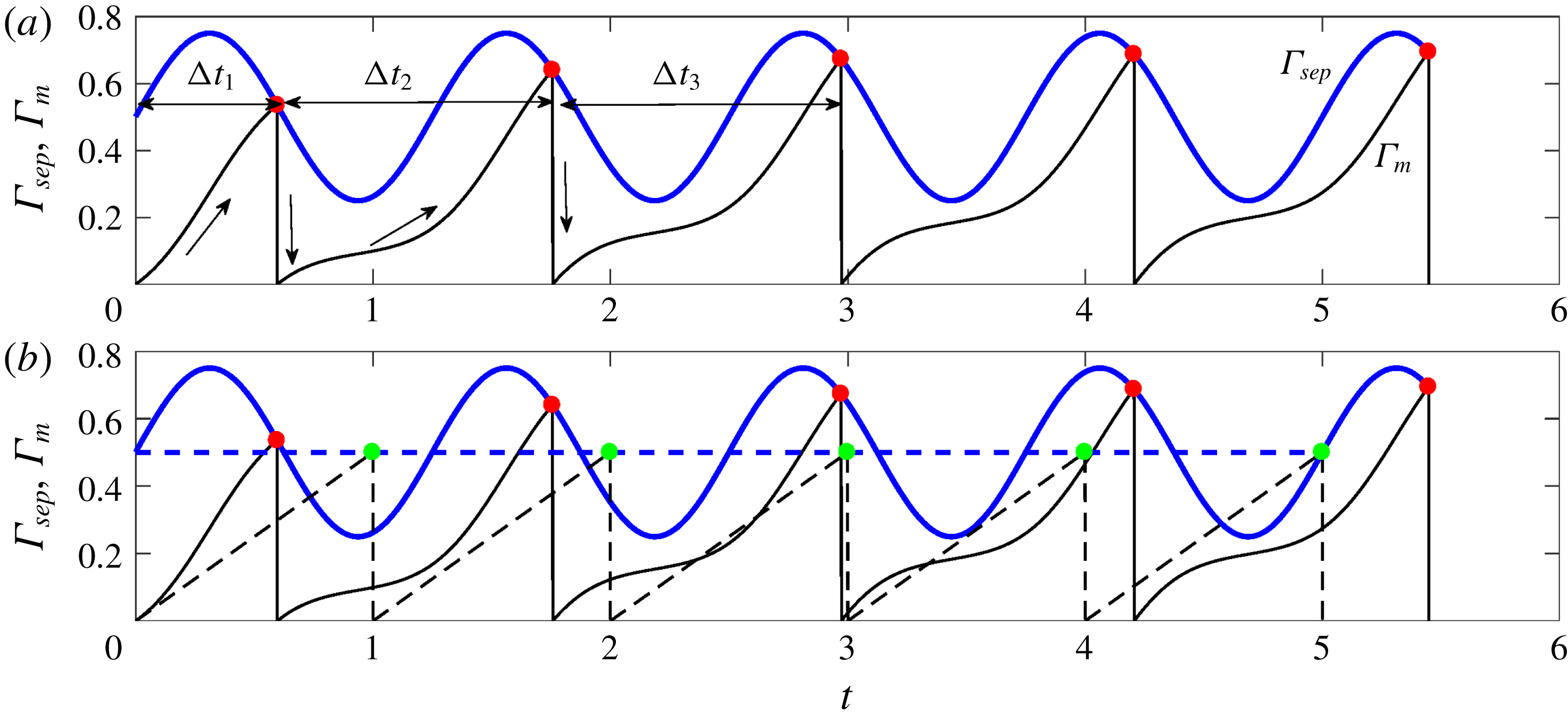
in our investigation. In figure 2(a), the evolution of
 $\unicode[STIX]{x1D6E4}_{m}$
(black curve) and
 $\unicode[STIX]{x1D6E4}_{sep}$
(blue curve) are plotted using (2.4) and (2.5) for
 $A=0.5,f=0.8$
. The shedding instances are marked using solid red circles, where
 $\unicode[STIX]{x1D6E4}_{m}=\unicode[STIX]{x1D6E4}_{sep}$
. At every shedding instance, the circulation of the next vortex is reset to zero. The time difference between two successive shedding events corresponds to the instantaneous vortex shedding time period and is marked as
 $\unicode[STIX]{x0394}t_{1},\unicode[STIX]{x0394}t_{2},\ldots \,$
. The subscript indicates the vortex number. Figure 2(b) shows a comparison of shedding instances between two amplitudes of velocity fluctuation. Dashed and solid curves correspond to
 $A=0$
and
 $A=0.5$
at
 $f=0.8$
respectively. It is seen that time instances of shedding (green and red circles for
 $A=0$
and
 $A=0.5$
respectively) are different for the two amplitudes. For
 $A=0$
, all the vortices are shed at a constant time interval equal to the steady-state shedding time period (
 $\unicode[STIX]{x0394}t_{st}$
). On the other hand, the instantaneous shedding time period varies with vortex number for
 $A=0.5$
.
(a) Time evolution of
 $\unicode[STIX]{x1D6E4}_{m}$
and
 $\unicode[STIX]{x1D6E4}_{sep}$
for
 $f=0.8$
and
 $A=0.5$
. Vortex shedding (firing) events are represented by solid red circles. During a firing event, circulation of the subsequent vortex is reset to zero. The time difference between consecutive firing,
 $\unicode[STIX]{x0394}t_{1},\unicode[STIX]{x0394}t_{2},\ldots ,$
represents the instantaneous vortex shedding time period. (b) Comparison of vortex shedding instances in the absence (
 $u^{\prime }=0$
, green circles) and presence (
 $f=0.8,A=0.5$
, red circles) of external excitation. Dashed and continuous lines indicate the evolution of
 $\unicode[STIX]{x1D6E4}_{m},\unicode[STIX]{x1D6E4}_{sep}$
for the above two cases respectively.

The process of vortex shedding defined by (2.4) and (2.5) is similar to the relaxation oscillator or ‘integrate and fire’ model, studied extensively for practical applications (Alstrøm, Christiansen & Levinsen Reference Alstrøm, Christiansen and Levinsen1988; Kirk & Stone Reference Kirk and Stone1997; Ernst, Pawelzik & Geisel Reference Ernst, Pawelzik and Geisel1998). In the simplest form, the model can be reduced to a circle map. Similarly, it can be seen in the following section (§ 2.1) that forced vortex shedding is also governed by a map equation that represents the shedding instances as phase points on a circle.
2.1 Derivation of the map equation
Let
 $t_{m-1}$
and
 $t_{m}$
be the shedding time instances of the
 $(m-1)$
th and
 $m$
th vortices respectively. The circulation strength of the
 $m$
th vortex is given by integrating (2.4):
 $$\begin{eqnarray}\unicode[STIX]{x1D6E4}_{m}(t_{m})-\unicode[STIX]{x1D6E4}_{m}(t_{m-1})=\int _{t_{m-1}}^{t_{m}}\frac{1}{2}[1+u^{\prime }(t)]^{2}\,\text{d}t.\end{eqnarray}$$
The circulation of the
 $m$
th vortex starts from zero (
 $\unicode[STIX]{x1D6E4}_{m}(t_{m-1})=0$
). Using
 $u^{\prime }=A\sin (2\unicode[STIX]{x03C0}ft+\unicode[STIX]{x1D719}_{0})$
in (2.6),
 $$\begin{eqnarray}\displaystyle \unicode[STIX]{x1D6E4}_{m}(t_{m}) & = & \displaystyle \frac{A^{2}(t_{m}-t_{m-1})}{4}-\frac{A^{2}[\sin (2\unicode[STIX]{x1D714}t_{m}+2\unicode[STIX]{x1D719}_{0})-\sin (2\unicode[STIX]{x1D714}t_{m-1}+2\unicode[STIX]{x1D719}_{0})]}{8\unicode[STIX]{x1D714}}\nonumber\\ \displaystyle & & \displaystyle -\,\frac{A[\cos (\unicode[STIX]{x1D714}t_{m}+\unicode[STIX]{x1D719}_{0})-\cos (\unicode[STIX]{x1D714}t_{m-1}+\unicode[STIX]{x1D719}_{0})]}{\unicode[STIX]{x1D714}}+\frac{(t_{m}-t_{m-1})}{2},\end{eqnarray}$$
where
 $\unicode[STIX]{x1D714}=2\unicode[STIX]{x03C0}f$
. At the time instant when the
 $m$
th vortex separates,
 $\unicode[STIX]{x1D6E4}_{m}(t_{m})=\unicode[STIX]{x1D6E4}_{sep}=(1+A\sin (2\unicode[STIX]{x03C0}ft_{m}+\unicode[STIX]{x1D719}_{0}))/2$
. Therefore (2.7) becomes
 $$\begin{eqnarray}\displaystyle & & \displaystyle (t_{m}-t_{m-1})\left(\frac{A^{2}}{4}+\frac{1}{2}\right)-\frac{A^{2}[\sin (2\unicode[STIX]{x1D714}t_{m}+2\unicode[STIX]{x1D719}_{0})-\sin (2\unicode[STIX]{x1D714}t_{m-1}+2\unicode[STIX]{x1D719}_{0})]}{8\unicode[STIX]{x1D714}}\nonumber\\ \displaystyle & & \displaystyle \quad -\,\frac{A[\cos (\unicode[STIX]{x1D714}t_{m}+\unicode[STIX]{x1D719}_{0})-\cos (\unicode[STIX]{x1D714}t_{m-1}+\unicode[STIX]{x1D719}_{0})]}{\unicode[STIX]{x1D714}}-\frac{1}{2}[A\sin (\unicode[STIX]{x1D714}t_{m}+\unicode[STIX]{x1D719}_{0})+1]=0.\end{eqnarray}$$
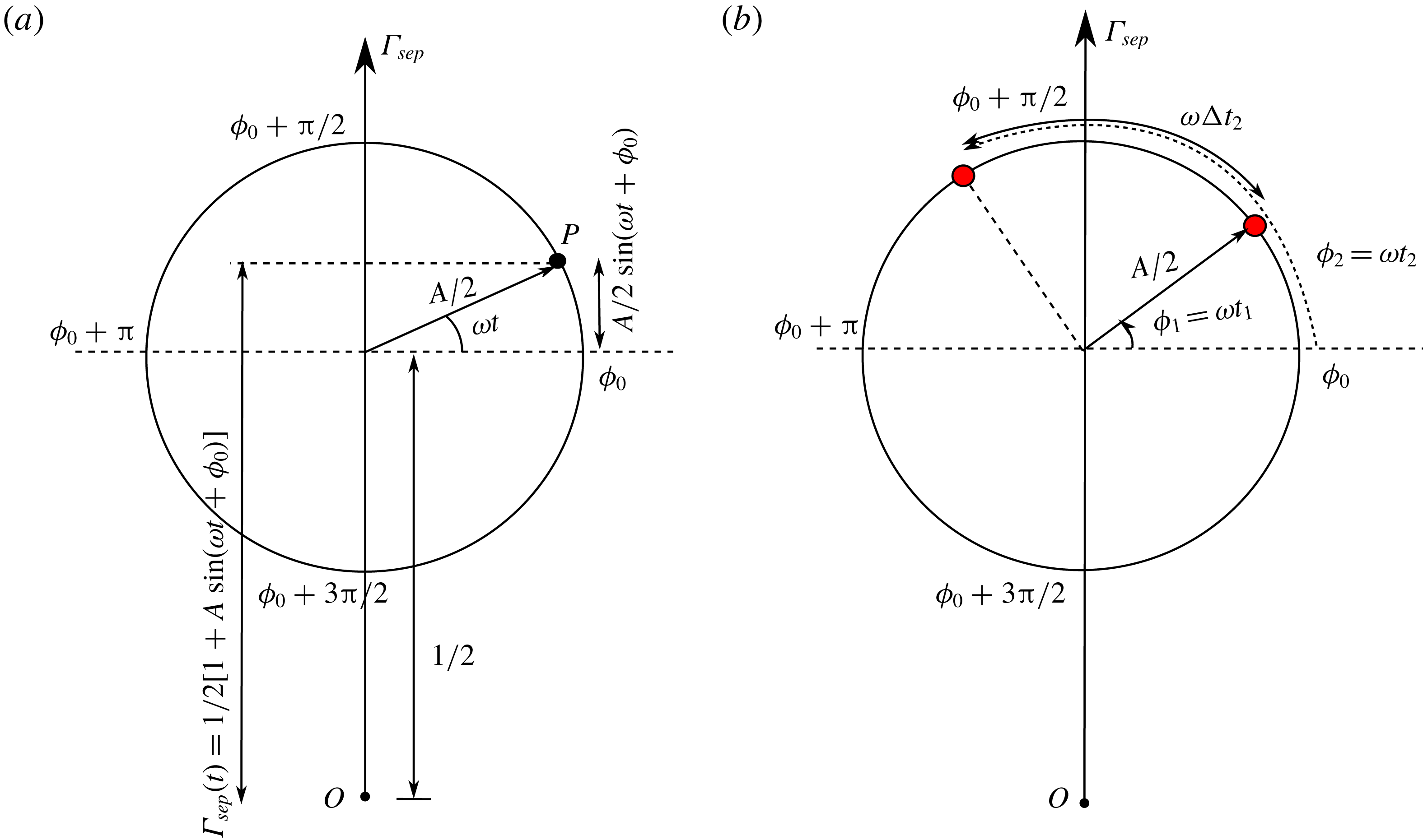
Representation of time instances of vortex shedding under forced excitation as phase points on a circle. (a) Harmonic fluctuations of threshold circulation
 $\unicode[STIX]{x1D6E4}_{sep}$
are represented as a circle of radius
 $A/2$
, with its centre displaced by
 $1/2$
along the vertical axis. At any time
 $t$
, the vertical distance of the phase point
 $P$
on the circle represents
 $\unicode[STIX]{x1D6E4}_{sep}(t)$
. (b) Phase points (red filled circles) correspond to vortex shedding time instances, where
 $\unicode[STIX]{x1D6E4}_{m}=\unicode[STIX]{x1D6E4}_{sep}$
.

Equation (2.8) represents an implicit difference relation for the vortex shedding time
 $t_{m}$
, given the time instance for the previous shedding
 $t_{m-1}$
. The harmonic terms in the equation constitute the nonlinearity of the implicit map. Furthermore, our interest lies in studying the vortex shedding time period. Hence, monitoring the instantaneous shedding period
 $\unicode[STIX]{x0394}t_{m}=t_{m}-t_{m-1}$
is more appropriate than the actual time instants. Therefore, it is convenient to represent the map iterates as phase points on a circle, illustrated in figure 3. For harmonic fluctuations,
 $\unicode[STIX]{x1D6E4}_{sep}$
can be represented as a circle (figure 3
a) of radius
 $A/2$
, with its centre displaced by a length
 $1/2$
from the origin
 $O$
on the vertical axis to satisfy (2.5). The evolution of
 $\unicode[STIX]{x1D6E4}_{sep}$
is related to the movement of point
 $P$
over the circle in the anticlockwise direction. At any instant of time, the location of
 $P$
is represented by the phase angle,
 $\unicode[STIX]{x1D719}=\unicode[STIX]{x1D714}t$
(measured with respect to the initial phase
 $\unicode[STIX]{x1D719}_{0}$
). The vertical distance of
 $P$
from the origin
 $O$
at any time
 $t$
corresponds to the value
 $\unicode[STIX]{x1D6E4}_{sep}(t)$
. Phase points in figure 3(b) (red filled circles) represent vortex shedding time instances, which correspond to
 $\unicode[STIX]{x1D6E4}_{m}=\unicode[STIX]{x1D6E4}_{sep}$
. These phase points at shedding time instances
 $t_{1},t_{2},\ldots \,$
correspond to the phase values
 $\unicode[STIX]{x1D719}_{1}=\unicode[STIX]{x1D714}t_{1},\unicode[STIX]{x1D719}_{2}=\unicode[STIX]{x1D714}t_{2},\ldots \,$
respectively with respect to
 $\unicode[STIX]{x1D719}_{0}$
. Therefore, from figure 3(b),
 $$\begin{eqnarray}\unicode[STIX]{x1D719}_{2}=\unicode[STIX]{x1D719}_{0}+\unicode[STIX]{x1D714}t_{2}=\unicode[STIX]{x1D719}_{1}+\unicode[STIX]{x1D714}\unicode[STIX]{x0394}t_{2},\end{eqnarray}$$
where
 $\unicode[STIX]{x1D719}_{1}=\unicode[STIX]{x1D719}_{0}+\unicode[STIX]{x1D714}t_{1}$
and
 $\unicode[STIX]{x0394}t_{2}=t_{2}-t_{1}$
. In general,
 $$\begin{eqnarray}\unicode[STIX]{x1D719}_{m}=\unicode[STIX]{x1D719}_{0}+\unicode[STIX]{x1D714}t_{m}=\unicode[STIX]{x1D719}_{m-1}+\unicode[STIX]{x1D714}\unicode[STIX]{x0394}t_{m}.\end{eqnarray}$$
With the above transformation, we now replace
 $\unicode[STIX]{x1D719}_{0}+\unicode[STIX]{x1D714}t_{m}$
,
 $\unicode[STIX]{x1D719}_{0}+\unicode[STIX]{x1D714}t_{m-1}$
and
 $\unicode[STIX]{x0394}t_{m}$
with
 $\unicode[STIX]{x1D719}_{m}$
,
 $\unicode[STIX]{x1D719}_{m-1}$
and
 $(\unicode[STIX]{x1D719}_{m}-\unicode[STIX]{x1D719}_{m-1})/\unicode[STIX]{x1D714}$
respectively in map (2.8) to obtain
 $$\begin{eqnarray}\displaystyle & & \displaystyle (\unicode[STIX]{x1D719}_{m-1}-\unicode[STIX]{x1D719}_{m})\left(\frac{A^{2}}{4}+\frac{1}{2}\right)+\unicode[STIX]{x03C0}f(A\sin \unicode[STIX]{x1D719}_{m}+1)\nonumber\\ \displaystyle & & \displaystyle \quad +\,\frac{A^{2}}{8}(\sin 2\unicode[STIX]{x1D719}_{m}-\sin 2\unicode[STIX]{x1D719}_{m-1})+A(\cos \unicode[STIX]{x1D719}_{m}-\cos \unicode[STIX]{x1D719}_{m-1})=0.\end{eqnarray}$$
For a given value of parameters
 $A,f$
and previous map variable
 $\unicode[STIX]{x1D719}_{m-1}$
, the iterate
 $\unicode[STIX]{x1D719}_{m}$
is obtained by solving the above implicit equation. The instantaneous shedding time period is computed as
 $\unicode[STIX]{x0394}t_{m}=(\unicode[STIX]{x1D719}_{m}-\unicode[STIX]{x1D719}_{m-1})/2\unicode[STIX]{x03C0}$
. The initial condition
 $\unicode[STIX]{x1D719}_{0}$
is specified in the interval
 $[0,2\unicode[STIX]{x03C0}]$
. Equation (2.11) is then solved to obtain
 $\unicode[STIX]{x1D719}_{1}$
. The shedding time period of the first vortex is calculated as
 $\unicode[STIX]{x0394}t_{1}=(\unicode[STIX]{x1D719}_{1}-\unicode[STIX]{x1D719}_{0})/2\unicode[STIX]{x03C0}$
. Before the next iterate
 $\unicode[STIX]{x1D719}_{2}$
is obtained from
 $\unicode[STIX]{x1D719}_{1}$
, we perform a modulo
 $2\unicode[STIX]{x03C0}$
operation on
 $\unicode[STIX]{x1D719}_{1}$
, since the implicit map (2.11) is
 $2\unicode[STIX]{x03C0}$
periodic in
 $\unicode[STIX]{x1D719}_{m-1}$
. The exercise is then repeated with modulo-operated
 $\unicode[STIX]{x1D719}_{1}$
to obtain
 $\unicode[STIX]{x1D719}_{2}$
and next higher iterates. Usage of the modulo operation restricts the range of the iterates
 $\unicode[STIX]{x1D719}_{m-1}$
to
 $[0,2\unicode[STIX]{x03C0}]$
, which allows for elegant discussion and interpretation of the results. The presence of the harmonic terms in the equation not only constitutes the nonlinearity of the map but also indicates the possibility of multiple solutions. In our case, the first root
 $\unicode[STIX]{x1D719}_{m}$
is the required solution. The
 $m$
th vortex is shed as soon as
 $\unicode[STIX]{x1D719}_{m}$
becomes the first root. The need to extract the first root requires the use of customized root finding methodology discussed in appendix A.
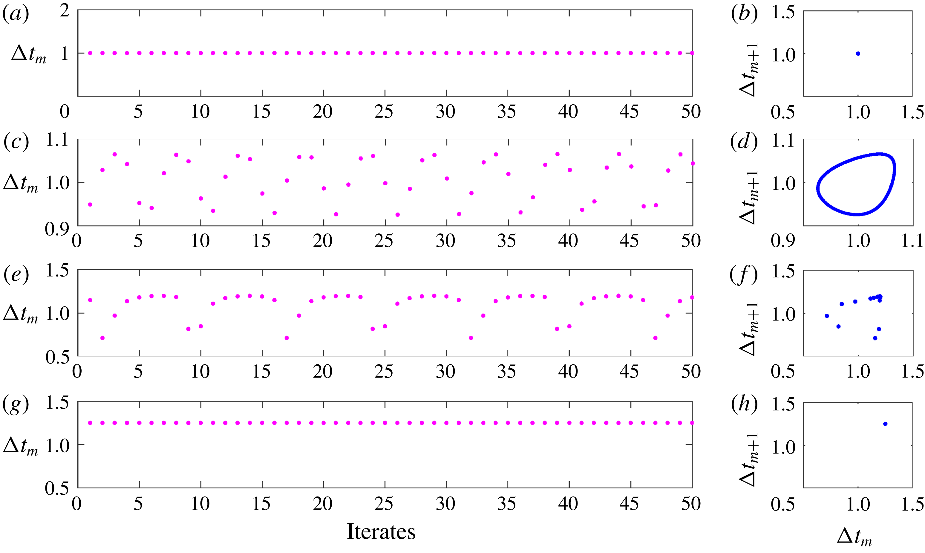
Plot showing the last 50 iterates (for clarity) of the instantaneous vortex shedding time period (a,c,e,g) and Poincaré maps (last 1000 iterates) between the
 $m$
th and
 $(m+1)$
th shedding period (b,d,f,h). Panels in each row from the top correspond to plots of increasing amplitudes: (a,b)
 $A=0$
, (c,d)
 $A=0.05$
, (e,f)
 $A=0.2$
and (g,h)
 $A=0.4$
. All the plots are obtained for frequency ratio
 $f=0.8$
.

2.2 Numerical results
We begin with presenting the results of numerical investigations to highlight the dynamical behaviour of the system under various forcing frequency ratios
 $f$
and amplitudes
 $A$
. They form the basis and motivation for our analytical study. Map equation (2.11) is solved for 2000 iterates, with
 $\unicode[STIX]{x1D719}_{0}=0$
. To eliminate the effect of transients, only the last 1000 iterates are used for the study. The results are found (not shown here) to be independent of the choice of
 $\unicode[STIX]{x1D719}_{0}$
. We choose
 $f=0.8$
, as lock-in (also termed synchronization in this paper) is expected to occur at frequencies close to natural frequency (
 $1/\unicode[STIX]{x1D6E5}_{st}$
) of the system. Amplitude
 $A$
is varied from 0 to 1. The results are shown in figure 4 in terms of instantaneous vortex shedding time period (a,c,e,g) and the corresponding Poincaré map between the
 $m$
th and
 $(m+1)$
th shedding period (b,d,f,h). In (a,c,e,g), the last 50 iterates are shown for clarity.
For
 $A=0$
(figure 4
a), we observe that vortices are shed at their natural vortex shedding time period (
 $\unicode[STIX]{x0394}t_{m}=1$
). For every iterate, the value of
 $\unicode[STIX]{x0394}t_{m}$
is the same, leading to a period-1 fixed point (Elaydi Reference Elaydi2007). In general, if
 $\unicode[STIX]{x0394}t_{m}$
repeats itself every
 $r$
iterates, it is termed a period-
 $r$
fixed point (also known as
 $r$
-periodic orbit). For higher amplitudes,
 $A=0.05$
and
 $A=0.2$
(figures 4
c and 4
e respectively), the fixed points appear to be of higher periodic nature; however, they are found to be not exactly repetitive through their Poincaré maps (discussed subsequently). For
 $A=0.4$
(figure 4
g), we again obtain a period-1 fixed point, with vortices shedding at the forcing frequency (
 $\unicode[STIX]{x0394}t_{m}=1/f$
) (unlike for
 $A=0$
). This represents lock-in.
Plot showing the last 1000 iterates of the instantaneous vortex shedding frequency (
 $1/\unicode[STIX]{x0394}t_{m}$
) with frequency ratio
 $f$
for two amplitudes (a)
 $A=0.07$
and (b)
 $A=0.1$
. The region of lock-in can be identified by straight lines, appearing around
 $f=1,2,3$
. Ratios in the figure indicate the occurrence of
 $1:1$
,
 $2:1$
and
 $3:1$
lock-in.

The above-described dynamics can also be indicated using Poincaré maps between
 $\unicode[STIX]{x0394}t_{m+1}$
and
 $\unicode[STIX]{x0394}t_{m}$
. The geometry of the Poincaré map indicates the period of the fixed point. For
 $A=0$
and
 $A=0.4$
, the fixed point is of period-1. Hence, the Poincaré map converges to a point (
 $\unicode[STIX]{x0394}t_{m+1}=\unicode[STIX]{x0394}t_{m}$
, see figure 4
b,h). On the other hand, the iterates densely fill a closed curve for
 $A=0.05$
(figure 4
d), indicating the quasi-periodic nature of the system. For higher amplitude,
 $A=0.2$
(figure 4
f), one observes discrete points, representing a higher-periodic solution. The above-described transition from an unforced to lock-in state through quasi-periodic behaviour was reported in experiments with low-density momentum-dominated jets (Li & Juniper Reference Li and Juniper2013a
).
Plot showing the last 1000 iterates of the instantaneous vortex shedding time period (
 $\unicode[STIX]{x0394}t_{m}$
) with amplitude
 $A$
for forcing frequency ratios (a)
 $f=0.8$
, (b)
 $f=0.9$
, (c)
 $f=1.1$
, (d)
 $f=1.2$
and (e)
 $f=3.2$
.
 $1:1$
lock-in is observed for panels (a–d). In panel (e), lock-in begins from
 $3:1$
state and ends in
 $1:1$
state as
 $A$
increases. Windows having higher-periodic oscillations are observed in panels (a,d,e). They are shown as insets.

Since the main aim of this paper is to identify the onset and extent of lock-in for various
 $A$
and
 $f$
analytically, it is important to understand the behaviour of
 $\unicode[STIX]{x0394}t_{m}$
with the above two parameters. This can be performed numerically in two steps: by varying (1) frequency ratio
 $f$
for a given value of
 $A$
and (2) amplitude
 $A$
for a given value of
 $f$
. Figure 5 shows the results of the last 1000 iterates of the instantaneous vortex shedding frequency (
 $1/\unicode[STIX]{x0394}t_{m}$
) with frequency ratio
 $f$
for two amplitudes
 $A=0.07$
(a) and
 $A=0.1$
(b). The region of lock-in can be identified by straight lines, appearing around
 $f=1,2,3$
. Near
 $f=1$
, the instantaneous shedding frequency
 $1/\unicode[STIX]{x0394}t_{m}=f$
, indicating that lock-in occurs with the forcing frequency. It is also observed that lock-in happens when the exciting frequency is around the higher harmonics of the natural vortex shedding frequency (
 $f\approx 2,3$
). In such cases, we observed a response (period-1 fixed point), at the subharmonics of the forcing frequency (
 $1/\unicode[STIX]{x0394}t_{m}=f/2,f/3$
). In general, when vortex shedding occurs at frequency
 $q$
(response), for an excitation frequency
 $p$
, the system is said to have attained
 $p:q$
lock-in (Pikovsky et al.
Reference Pikovsky, Rosenblum and Kurths2003). Hence, figure 5 shows the occurrence of
 $1:1$
,
 $2:1$
and
 $3:1$
lock-in. The extent of lock-in increases with higher frequency ratios. The results are qualitatively similar for excitation with higher amplitudes
 $A$
, while quantitatively the extent of lock-in is larger.
We continue with the second step, where we vary the amplitude
 $A$
between 0 and 1 for five fixed frequency ratios
 $f=0.8,0.9,1.1,1.2$
and
 $3.2$
, all close to the natural vortex shedding frequency and its harmonics. The results are shown in figure 6. A vortex sheds at its natural time period for
 $A=0$
. When
 $A$
is increased to slightly greater than zero, we observe that the iterates densely fill a range of shedding time periods, indicating the quasi-periodic nature. On further increase in
 $A$
, higher-periodic solutions appear, culminating in lock-in. The region of lock-in is identified by a horizontal straight line in the sub-figures. Since in figure 6(a–d),
 $f$
is close to 1,
 $1:1$
lock-in is observed. It is interesting to note that there is an upper limit on amplitude, beyond which lock-in ceases to exist (de-lock-in). A higher-periodic solution occurs. The amplitude range of lock-in is found to increase with the closeness of
 $f$
to 1. Another important observation is the occurrence of windows of higher periods (see the insets of figure 6
a,d,e) in the region where quasi-periodic oscillations are present.
The above discussion relates to cases where the exciting frequency is close to the natural vortex shedding frequency. Interesting dynamics occur when
 $f$
is close to a higher harmonic of
 $\unicode[STIX]{x0394}t_{st}$
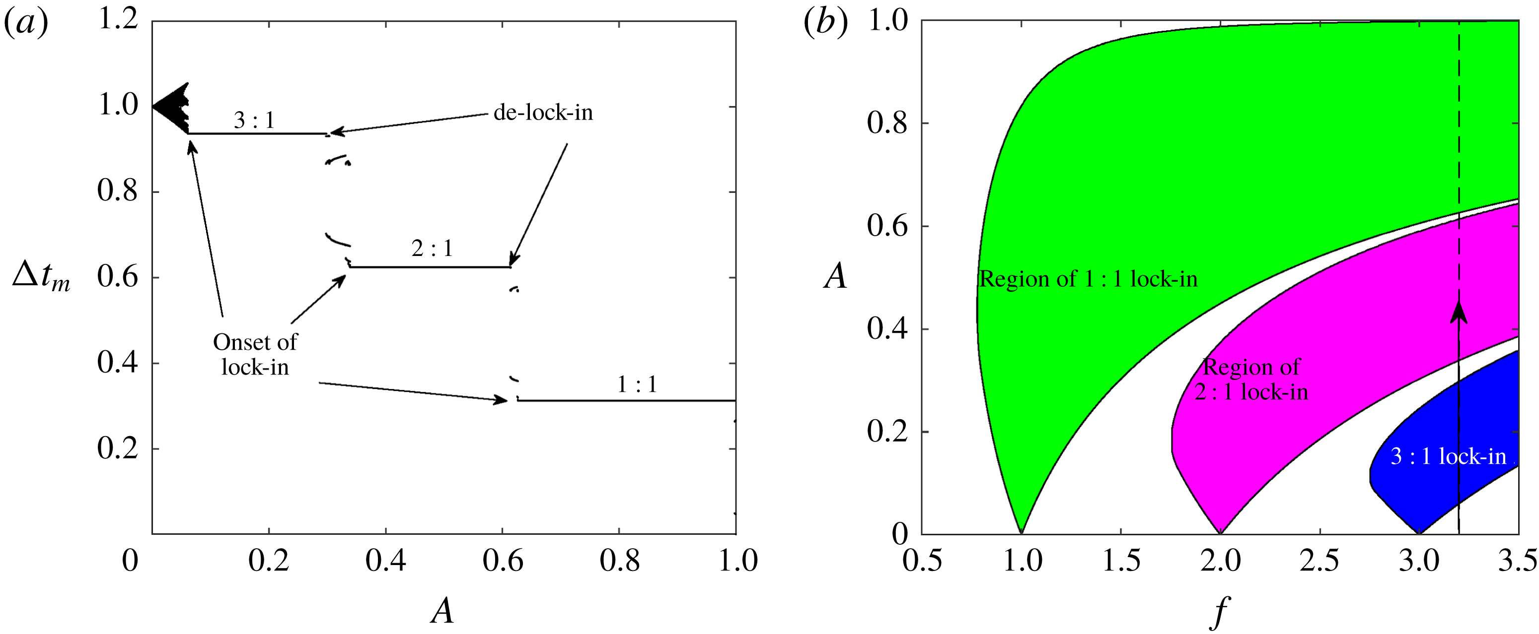
: one such case is illustrated through figure 6(e). It represents the iterates for
 $\unicode[STIX]{x0394}t_{m}$
at
 $f=3.2$
. In this plot, lock-in can be observed at three different values of
 $\unicode[STIX]{x0394}t_{m}$
. For low-amplitude forcing, the vortex shedding time period
 $\unicode[STIX]{x0394}t_{m}$
locks-in to
 $3/f$
(
 $3:1$
lock-in). As
 $A$
increases, de-lock-in from
 $3:1$
occurs and the shedding time period locks-in to
 $2/f$
and then eventually to
 $1/f$
. Hence, from
 $3:1$
lock-in, the system reaches a
 $1:1$
lock-in state. The extent of these lock-in states is indicated by the three plateau lines.
To summarize, we have made the following important observations from the numerical simulations.
(i) Lock-in is identified as a period-1 fixed point, with the relation between the response and forcing frequencies at
$q$
and
$p$
respectively (
$p:q$
lock-in).(ii) There is a range of
$f$
for a fixed
$A$
and range of
$A$
for a fixed
$f$
where lock-in is observed. Although the former is not surprising, the latter result calls for further investigation.(iii) When
$f$
is far away from the natural vortex shedding frequency, higher-order lock-in first occurs, which eventually culminates in
$1:1$
lock-in, as the amplitude is increased.


In this paper, we have made an attempt to understand the above behaviour analytically and obtain general results, which can be verified through experiments.
3 Extraction of analytical solutions
Our first step in the analytical investigation is to predict the onset and termination of lock-in. To begin, we identify the periodic solutions of (2.11). As said before, a
 $p:q$
lock-in is a periodic solution, where
 $f/(1/\unicode[STIX]{x0394}t_{m})=p/q$
. This indicates that
 $\unicode[STIX]{x1D714}\unicode[STIX]{x0394}t_{m}=2\unicode[STIX]{x03C0}f\unicode[STIX]{x0394}t_{m}=2\unicode[STIX]{x03C0}p/q$
. Hence for
 $p:q$
lock-in, equation (2.10) becomes
 $\unicode[STIX]{x1D719}_{m}=\unicode[STIX]{x1D719}_{m-1}+2\unicode[STIX]{x03C0}p/q$
. Substituting in (2.11), we obtain
 $$\begin{eqnarray}\displaystyle & & \displaystyle -\frac{2\unicode[STIX]{x03C0}p}{q}\left(\frac{A^{2}}{4}+\frac{1}{2}\right)+\unicode[STIX]{x03C0}f\left[A\sin \left(\unicode[STIX]{x1D719}_{m-1}+2\unicode[STIX]{x03C0}\frac{p}{q}\right)+1\right]\nonumber\\ \displaystyle & & \displaystyle \quad +\,\frac{\displaystyle A^{2}\left[\sin 2\left(\unicode[STIX]{x1D719}_{m-1}+2\unicode[STIX]{x03C0}\frac{p}{q}\right)-\sin 2\unicode[STIX]{x1D719}_{m-1}\right]}{8}\nonumber\\ \displaystyle & & \displaystyle \quad +\,A\left[\cos \left(\unicode[STIX]{x1D719}_{m-1}+2\unicode[STIX]{x03C0}\frac{p}{q}\right)-\cos (\unicode[STIX]{x1D719}_{m-1})\right]=0.\end{eqnarray}$$
We observed that in the current analytical framework, solutions for a general
 $p:1$
lock-in state can be extracted. Moreover, these lock-in states are observed in our numerical simulations (figure 5). Hence, we restrict our investigation to the
 $p:1$
lock-in phenomenon.
3.1
$p:1$
lock-in

Substituting
 $q=1$
, equation (3.1) becomes
 $$\begin{eqnarray}-2\unicode[STIX]{x03C0}\left(\frac{A^{2}}{4}+\frac{1}{2}\right)+\frac{\unicode[STIX]{x03C0}f}{p}[A\sin (\unicode[STIX]{x1D719}_{m-1})+1]=0.\end{eqnarray}$$
For a given value of
 $f/p$
and
 $A$
, the lock-in state of the system is described by
 $\unicode[STIX]{x1D719}_{m-1}$
. The above equation is used to find an explicit expression for
 $\sin \unicode[STIX]{x1D719}_{m-1}$
. A solution for
 $\unicode[STIX]{x1D719}_{m-1}$
exists when
 $|\!\sin \unicode[STIX]{x1D719}_{m-1}|\leqslant 1$
. Therefore, lock-in occurs when the following inequality is satisfied:
 $$\begin{eqnarray}|\text{sin}\,\unicode[STIX]{x1D719}_{m-1}|=\left|\frac{\displaystyle \left[A^{2}+2\left(1-\frac{f}{p}\right)\right]}{2A(f/p)}\right|\leqslant 1.\end{eqnarray}$$
It is observed that the solution of
 $\sin \unicode[STIX]{x1D719}_{m-1}$
depends on
 $A$
and
 $f/p$
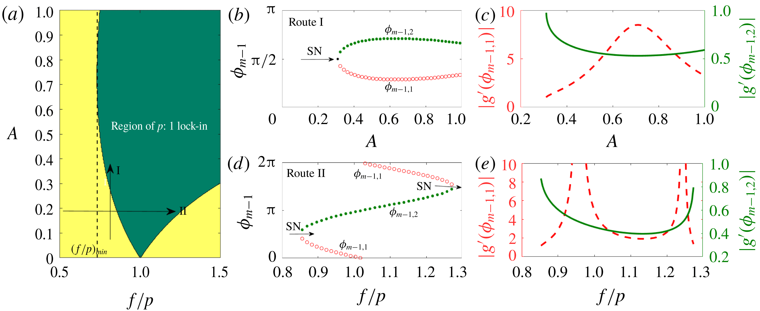
. Figure 7(a) represents the region of
 $p:1$
lock-in (shown in green) for the excitation parameters,
 $A$
and
 $f/p$
. Firstly, we notice that the boundary of lock-in is asymmetric with respect to
 $f/p=1$
. Secondly, there is a lower limit for
 $f/p$
(termed
 $(f/p)_{min}$
and marked with a vertical dashed line) below which
 $p:1$
lock-in does not occur for any amplitude of excitation. Lastly, once lock-in is established at a particular amplitude, the system remains in the locked-in state, for all higher amplitudes (up to
 $A=1$
is considered in this paper). However, as discussed towards the end of § 2.2, there is an upper limit on the amplitude (less than 1) above which de-lock-in occurs (see figure 6). In the next section, we perform an analytical investigation to explain the above observations.
3.2 Nature of bifurcation and stability
Inside the region of lock-in, we have two fixed points for
 $\unicode[STIX]{x1D719}_{m-1}$
in
 $[0,2\unicode[STIX]{x03C0}]$
, since
 $\sin \unicode[STIX]{x1D719}_{m-1}=\sin (\unicode[STIX]{x03C0}-\unicode[STIX]{x1D719}_{m-1})$
. They are
 $$\begin{eqnarray}\displaystyle & \displaystyle \unicode[STIX]{x1D719}_{m-1,1}=\arcsin \left(\frac{\displaystyle \left[A^{2}+2\left(1-\frac{f}{p}\right)\right]}{2A(f/p)}\right), & \displaystyle\end{eqnarray}$$
 $$\begin{eqnarray}\displaystyle & \displaystyle \unicode[STIX]{x1D719}_{m-1,2}=\unicode[STIX]{x03C0}-\arcsin \left(\frac{\displaystyle \left[A^{2}+2\left(1-\frac{f}{p}\right)\right]}{2A(f/p)}\right), & \displaystyle\end{eqnarray}$$
where subscripts
 $1$
and
 $2$
represent the two fixed points. These fixed points are plotted for various amplitudes
 $A$
with a given
 $f/p=0.8$
(termed as route I) in figure 7(b) and vice versa (
 $A=0.2$
) in figure 7(d) (route II). Routes I and II are indicated as vertical and horizontal arrows respectively in figure 7(a). In the former, we observe that for low amplitudes (
 $A<0.31$
), no fixed point exists. Two fixed points (solid green and hollow red curves) appear as one crosses the lock-in boundary. In the latter case (figure 7
d), for low (
 ${<}0.85$
) and high (
 ${>}1.28$
) values of
 $f/p$
, there are no lock-in solutions. As one increases the value of
 $f/p$
from the lower side (
 $f/p<1$
), lock-in occurs by the appearance of two fixed points. On the other side of
 $f/p=1$
, these two fixed points coalesce and de-lock-in occurs. In both cases new fixed points appear when the boundary of lock-in is crossed, which indicates the possibility of saddle-node bifurcation. However, a confirmation can be made by analysing the stability of the fixed points.
(a) A representation of the region of
 $p:1$
lock-in for the parameters,
 $A$
and
 $f/p$
. Green and yellow colours indicate the regions of lock-in and no-lock-in states respectively. Vertical and horizontal arrows indicate routes I and II, which correspond to increasing amplitude at constant excitation frequency and vice versa respectively. Period-1 fixed points
 $\unicode[STIX]{x1D719}_{m-1,1},\unicode[STIX]{x1D719}_{m-1,2}$
of (2.11) for (b) various amplitudes at
 $f/p=0.8$
(route I) and (d) various
 $f/p$
at
 $A=0.2$
(route II). Two fixed points are present inside the region of lock-in. Green solid and red hollow circles indicate stable and unstable fixed points respectively. SN represents a saddle-node bifurcation. (c),(e) The variation of
 $|g^{\prime }(\unicode[STIX]{x1D719}_{m-1,1})|,|g^{\prime }(\unicode[STIX]{x1D719}_{m-1,2})|$
corresponding to panels (b) and (d) respectively. Green solid and red dashed curves are associated with stable and unstable fixed points respectively.

The fixed points
 $\unicode[STIX]{x1D719}_{m-1,1},\unicode[STIX]{x1D719}_{m-1,2}$
are the period-1 solutions of (2.11). Equation (2.11) is an implicit difference equation and therefore the stability of its fixed points is obtained by the following procedure. It is known that the stability of an explicit difference equation of the form
 $\unicode[STIX]{x1D719}_{m}=g(\unicode[STIX]{x1D719}_{m-1})$
is found by evaluating
 $$\begin{eqnarray}g^{\prime }(\unicode[STIX]{x1D719}_{m-1})|_{\unicode[STIX]{x1D719}_{m-1}^{\ast }}=\left.\frac{\text{d}g(\unicode[STIX]{x1D719}_{m-1})}{\text{d}\unicode[STIX]{x1D719}_{m-1}}\right|_{\unicode[STIX]{x1D719}_{m-1}^{\ast }}=\left.\frac{\text{d}\unicode[STIX]{x1D719}_{m}}{\text{d}\unicode[STIX]{x1D719}_{m-1}}\right|_{\unicode[STIX]{x1D719}_{m-1}^{\ast }}\!,\end{eqnarray}$$
where
 $\unicode[STIX]{x1D719}_{m-1}^{\ast }$
is a period-1 fixed point given by
 $\unicode[STIX]{x1D719}_{m-1}^{\ast }=g(\unicode[STIX]{x1D719}_{m-1}^{\ast })$
. Here,
 $\unicode[STIX]{x1D719}_{m-1}^{\ast }$
is asymptotically stable if
 $|g^{\prime }(\unicode[STIX]{x1D719}_{m-1}^{\ast })|=|\text{d}\unicode[STIX]{x1D719}_{m}/\text{d}\unicode[STIX]{x1D719}_{m-1}|_{\unicode[STIX]{x1D719}_{m-1}^{\ast }}<1$
. Also,
 $\text{d}\unicode[STIX]{x1D719}_{m}/\text{d}\unicode[STIX]{x1D719}_{m-1}$
is evaluated from the implicit difference equation (2.11), which is of the form
 $F(\unicode[STIX]{x1D719}_{m},\unicode[STIX]{x1D719}_{m-1})=0$
. The expression for
 $\text{d}\unicode[STIX]{x1D719}_{m}/\text{d}\unicode[STIX]{x1D719}_{m-1}$
in terms of partial derivatives of
 $F=0$
is given by (intermediate steps are shown in appendix B)
 $$\begin{eqnarray}\left.\frac{\text{d}\unicode[STIX]{x1D719}_{m}}{\text{d}\unicode[STIX]{x1D719}_{m-1}}\right|_{\unicode[STIX]{x1D719}_{m-1}^{\ast }}=\left.\frac{-\unicode[STIX]{x2202}F/\unicode[STIX]{x2202}\unicode[STIX]{x1D719}_{m-1}}{\unicode[STIX]{x2202}F/\unicode[STIX]{x2202}\unicode[STIX]{x1D719}_{m}}\right|_{\unicode[STIX]{x1D719}_{m-1}^{\ast }},\end{eqnarray}$$
where
 $$\begin{eqnarray}\displaystyle & \displaystyle \left.\frac{\unicode[STIX]{x2202}F}{\unicode[STIX]{x2202}\unicode[STIX]{x1D719}_{m-1}}\right|_{\unicode[STIX]{x1D719}_{m-1}^{\ast }}=\left(\frac{A^{2}}{4}+\frac{1}{2}\right)-\frac{A^{2}}{4}\cos 2\unicode[STIX]{x1D719}_{m-1}^{\ast }+A\sin \unicode[STIX]{x1D719}_{m-1}^{\ast }, & \displaystyle\end{eqnarray}$$
 $$\begin{eqnarray}\displaystyle & \displaystyle \left.\frac{\unicode[STIX]{x2202}F}{\unicode[STIX]{x2202}\unicode[STIX]{x1D719}_{m}}\right|_{\unicode[STIX]{x1D719}_{m-1}^{\ast }}=-\left(\frac{A^{2}}{4}+\frac{1}{2}\right)+\unicode[STIX]{x03C0}fA\cos \unicode[STIX]{x1D719}_{m-1}^{\ast }+\frac{A^{2}}{4}\cos 2\unicode[STIX]{x1D719}_{m-1}^{\ast }-A\sin \unicode[STIX]{x1D719}_{m-1}^{\ast }. & \displaystyle\end{eqnarray}$$
In the present case
 $\unicode[STIX]{x1D719}_{m-1}^{\ast }$
represents either
 $\unicode[STIX]{x1D719}_{m-1,1}$
or
 $\unicode[STIX]{x1D719}_{m-1,2}$
(3.4) and (3.5). Using the above expressions,
 $|g^{\prime }(\unicode[STIX]{x1D719}_{m-1}^{\ast })|$
is evaluated for the two fixed points to determine their stability. The results are shown in figures 7(c) and 7(e) respectively for the case where
 $A$
(
 $f/p=0.8$
) and
 $f/p$
(
 $A=0.2$
) are varied. In both cases, we observe that for one of the fixed points
 $\unicode[STIX]{x1D719}_{m-1,2}$
,
 $|g^{\prime }(\unicode[STIX]{x1D719}_{m-1}^{\ast })|<1$
(green solid curve) indicating it to be stable. The other fixed point
 $\unicode[STIX]{x1D719}_{m-1,1}$
(red dashed curve) is found to be unstable. Therefore, we confirm that indeed saddle-node bifurcation occurs at the lock-in boundary.
In the past, extensive investigations (Balanov et al.
Reference Balanov, Janson, Postnov and Sosnovtseva2008) have indicated that the route to forced lock-in occurs via a saddle-node (near
 $f=1$
) or a torus death (far from
 $f=1$
) bifurcation. Numerical simulations of a forced VDP oscillator and experimental observations of Li & Juniper (Reference Li and Juniper2013a
) also indicate the presence of the two routes. From our Poincaré map of the numerical simulations (figure 4
b,d,f,h), we observe that as the excitation amplitude is increased, quasi-periodic solutions appear (panel d), which break down to a higher-periodic solution (panel f). This higher-periodic solution transitions to a period-1 (panel h) lock-in state. As representative of torus death bifurcation, we did not observe from our numerical simulations, the size of the torus decreasing gradually and leading to a lock-in state. Currently, the reason for the absence of torus death bifurcation in this model is unknown. Investigation on this important aspect can be taken up as future work.
3.3 Analytical determination of the lock-in boundary
We next move onto obtaining analytical expressions for the lock-in boundary. We perform this in two steps. First, we determine the lower limit of forcing frequency
 $(f/p)_{min}$
below which lock-in does not occur for any forcing amplitude. This is followed by obtaining the analytical expressions for the critical amplitude above which lock-in occurs for
 $f/p>(f/p)_{min}$
.
We begin from (3.2), which governs the solution for
 $p:1$
lock-in. The equation is quadratic in
 $A$
and its roots for a particular value of
 $f/p$
represent the range of amplitude for which vortex shedding exhibits
 $p:1$
lock-in. The solutions for
 $A$
are
 $$\begin{eqnarray}A_{1,2}=\frac{f}{p}\sin (\unicode[STIX]{x1D719}_{m-1})\pm \left[\left(\frac{f}{p}\right)^{2}\sin ^{2}(\unicode[STIX]{x1D719}_{m-1})-2\left(1-\frac{f}{p}\right)\right]^{1/2},\end{eqnarray}$$
where, for a given value of
 $f/p$
,
 $A_{1}$
and
 $A_{2}$
are two branches of solutions dependent on
 $\unicode[STIX]{x1D719}_{m-1}$
. For
 $A_{1}$
and
 $A_{2}$
to be real, the following condition must be satisfied:
 $$\begin{eqnarray}\left(\frac{f}{p}\right)^{2}\sin ^{2}(\unicode[STIX]{x1D719}_{m-1})\geqslant 2\left(1-\frac{f}{p}\right),\end{eqnarray}$$
which can be written as a quadratic inequality in
 $f/p$
 $$\begin{eqnarray}\sin ^{2}\unicode[STIX]{x1D719}_{m-1}\left(\frac{f}{p}\right)^{2}+2\left(\frac{f}{p}\right)-2\geqslant 0.\end{eqnarray}$$
The product of the roots of the above inequality is
 $-2/(\sin \unicode[STIX]{x1D719}_{m-1})^{2}$
, which is negative, indicating roots of opposite signs. Considering the physically relevant positive root, we have
 $$\begin{eqnarray}\frac{f}{p}\geqslant \left(\frac{f}{p}\right)_{cr}=\frac{(-1+[1+2\sin ^{2}\unicode[STIX]{x1D719}_{m-1}]^{1/2})}{\sin ^{2}\unicode[STIX]{x1D719}_{m-1}}.\end{eqnarray}$$
The lowest value of
 $(f/p)_{cr}$
for which lock-in occurs depends on
 $\unicode[STIX]{x1D719}_{m-1}$
. Therefore, obtaining the minimum of
 $(f/p)_{cr}$
with respect to
 $\unicode[STIX]{x1D719}_{m-1}$
provides the global minimum of
 $f/p$
above which lock-in exists. In the
 $(f/p)_{cr}$
–
 $\unicode[STIX]{x1D719}_{m-1}$
plane, the extremum of
 $(f/p)_{cr}$
exists at the location where the first derivative of (3.13) is zero, which leads to
 $$\begin{eqnarray}\frac{\text{d}(f/p)_{cr}}{\text{d}\unicode[STIX]{x1D719}_{m-1}}=\frac{2\cos \unicode[STIX]{x1D719}_{m-1}}{\sin ^{3}\unicode[STIX]{x1D719}_{m-1}}+\frac{2\cos \unicode[STIX]{x1D719}_{m-1}\sin ^{2}\unicode[STIX]{x1D719}_{m-1}-(2+4\sin ^{2}\unicode[STIX]{x1D719}_{m-1})\cos \unicode[STIX]{x1D719}_{m-1}}{\sin ^{3}\unicode[STIX]{x1D719}_{m-1}\sqrt{1+2\sin ^{2}\unicode[STIX]{x1D719}_{m-1}}}=0.\end{eqnarray}$$
A solution exist for
 $\cos \unicode[STIX]{x1D719}_{m-1}=0$
, indicating
 $\unicode[STIX]{x1D719}_{m-1}=\unicode[STIX]{x03C0}/2,3\unicode[STIX]{x03C0}/2$
. The second derivative of
 $(f/p)_{cr}$
is shown to be positive at the above locations of
 $\unicode[STIX]{x1D719}_{m-1}$
(details are presented in appendix C). Therefore it is concluded that
 $(f/p)_{cr}$
is the minimum at
 $\unicode[STIX]{x1D719}_{m-1}=\unicode[STIX]{x03C0}/2,3\unicode[STIX]{x03C0}/2$
. Using (3.13), the global minimum
 $(f/p)_{min}$
of the frequency ratio above which
 $p:1$
lock-in can occur is
 $$\begin{eqnarray}(f/p)_{min}=\sqrt{3}-1.\end{eqnarray}$$
The minimum value of the frequency ratio
 $f$
occurs for
 $1:1$
lock-in. Therefore, in a combustor, vortex shedding does not lock-in with a particular acoustic mode even for a large amplitude of oscillation, if the frequency of the latter is less than
 $(\sqrt{3}-1)/\unicode[STIX]{x0394}t_{st}$
. On the other hand, there is no upper limit on the frequency ratio, implying that if the acoustic frequency in a combustor is greater than the natural vortex shedding frequency, lock-in occurs eventually.
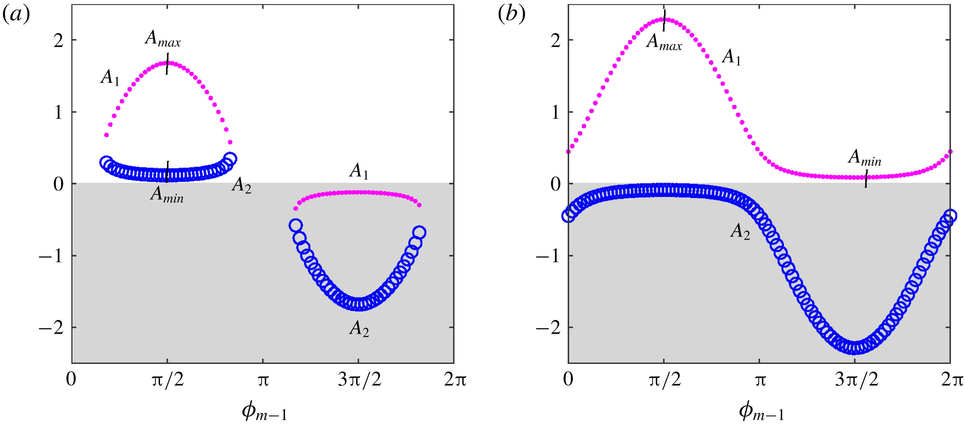
Variation of
 $A_{1}$
(pink dots) and
 $A_{2}$
(blue hollow circles) with
 $\unicode[STIX]{x1D719}_{m-1}$
for (a)
 $f/p=0.9$
and (b)
 $f/p=1.1$
. Regions of physically relevant positive values of
 $A_{1},A_{2}$
are unshaded.
 $A_{max}$
and
 $A_{min}$
correspond to the physically relevant maximum and minimum values respectively for
 $A_{1},A_{2}$
.

For
 $f/p>(f/p)_{min}$
, we obtain two real solutions for
 $A_{1,2}=A_{1},A_{2}$
(3.10). Figure 8 shows the plot
 $A_{1},A_{2}$
(in pink dots and blue hollow circles respectively) with
 $\unicode[STIX]{x1D719}_{m-1}$
. The curves are qualitatively different for
 $f/p<1$
(panel a),
 $f/p>1$
(panel b). As before, the local extrema in the
 $A_{1,2}$
–
 $\unicode[STIX]{x1D719}_{m-1}$
plane allow one to identify the global minimum and maximum amplitudes, between which lock-in occurs. The extrema are obtained by equating the derivative of (3.10) with respect to
 $\unicode[STIX]{x1D719}_{m-1}$
to zero:
 $$\begin{eqnarray}\frac{\text{d}A_{1,2}}{\text{d}\unicode[STIX]{x1D719}_{m-1}}=\frac{f}{p}\cos (\unicode[STIX]{x1D719}_{m-1})\pm \frac{f^{2}\sin (\unicode[STIX]{x1D719}_{m-1})\cos (\unicode[STIX]{x1D719}_{m-1})}{\displaystyle p^{2}\left[\left(\frac{f}{p}\right)^{2}\sin ^{2}(\unicode[STIX]{x1D719}_{m-1})-2\left(1-\frac{f}{p}\right)\right]^{1/2}}=0.\end{eqnarray}$$
The above equation is satisfied for
 $\cos (\unicode[STIX]{x1D719}_{m-1})=0$
, implying
 $\unicode[STIX]{x1D719}_{m-1}=\unicode[STIX]{x03C0}/2,3\unicode[STIX]{x03C0}/2$
. Figure 8 shows the occurrence of extrema at the above values. At the locations of extrema, the solutions
 $A_{1,2}$
become
 $$\begin{eqnarray}\displaystyle & \displaystyle A_{1,2}|_{ext}=\frac{f}{p}\pm \left[\left(\frac{f}{p}\right)^{2}-2\left(1-\frac{f}{p}\right)\right]^{1/2},\quad \text{at }\unicode[STIX]{x1D719}_{m-1}=\frac{\unicode[STIX]{x03C0}}{2}, & \displaystyle\end{eqnarray}$$
 $$\begin{eqnarray}\displaystyle & \displaystyle A_{1,2}|_{ext}=-\frac{f}{p}\pm \left[\left(\frac{f}{p}\right)^{2}-2\left(1-\frac{f}{p}\right)\right]^{1/2},\quad \text{at }\unicode[STIX]{x1D719}_{m-1}=\frac{3\unicode[STIX]{x03C0}}{2}, & \displaystyle\end{eqnarray}$$
where
 $A_{1,2}|_{ext}$
denotes the extrema of
 $A_{1,2}$
. The nature of the extrema (maxima or minima) is obtained from the sign of the second derivative
 $(\text{d}^{2}A_{1,2}/\text{d}\unicode[STIX]{x1D719}_{m-1}^{2})$
at
 $\unicode[STIX]{x1D719}_{m-1}=\unicode[STIX]{x03C0}/2,3\unicode[STIX]{x03C0}/2$
:
 $$\begin{eqnarray}\displaystyle & \displaystyle \frac{\text{d}^{2}A_{1,2}}{\text{d}\unicode[STIX]{x1D719}_{m-1}^{2}}=-\frac{f}{p}\mp \frac{f^{2}}{\displaystyle p^{2}\left[\left(\frac{f}{p}\right)^{2}-2\left(1-\frac{f}{p}\right)\right]^{1/2}},\quad \text{at }\unicode[STIX]{x1D719}_{m-1}=\frac{\unicode[STIX]{x03C0}}{2} & \displaystyle\end{eqnarray}$$
 $$\begin{eqnarray}\displaystyle & \displaystyle \frac{\text{d}^{2}A_{1,2}}{\text{d}\unicode[STIX]{x1D719}_{m-1}^{2}}=\frac{f}{p}\mp \frac{f^{2}}{\displaystyle p^{2}\left[\left(\frac{f}{p}\right)^{2}-2\left(1-\frac{f}{p}\right)\right]^{1/2}},\quad \text{at }\unicode[STIX]{x1D719}_{m-1}=\frac{3\unicode[STIX]{x03C0}}{2}. & \displaystyle\end{eqnarray}$$
Appendix C gives the details of the derivation of the above expressions. Although the solutions
 $A_{1,2}$
are real, they are physically relevant for positive values. Hence, the extrema of
 $A_{1},A_{2}$
, which occur in the unshaded region of figure 8 represent the required solution. Since the nature of
 $A_{1,2}$
is different for
 $f/p<1$
and
 $f/p>1$
, the analyses to determine the amplitude boundary are performed separately.
3.3.1 Condition
$f/p<1$

We observe that for
 $f/p<1$
,
 $1-f/p>0$
leading to the term
 $[(f/p)^{2}-2(1-f/p)]^{1/2}$
less than
 $f/p$
. Hence, at
 $\unicode[STIX]{x1D719}_{m-1}=3\unicode[STIX]{x03C0}/2$
,
 $A_{1,2}|_{ext}$
is negative (observed in figure 8
a). Then the physically relevant extrema lie at
 $\unicode[STIX]{x1D719}_{m-1}=\unicode[STIX]{x03C0}/2$
. Equation (3.19) indicates that
 $\text{d}^{2}A_{1}/\text{d}\unicode[STIX]{x1D719}_{m-1}^{2}<0$
and
 $\text{d}^{2}A_{2}/\text{d}\unicode[STIX]{x1D719}_{m-1}^{2}>0$
at
 $\unicode[STIX]{x1D719}_{m-1}=\unicode[STIX]{x03C0}/2$
based on the previous statements. Hence the minimum
 $(A_{min})$
and maximum
 $(A_{max})$
value of
 $A_{1,2}$
between which lock-in occurs lies on the curves
 $A_{2}$
and
 $A_{1}$
respectively. Therefore,
 $$\begin{eqnarray}\displaystyle & \displaystyle A_{min}=\frac{f}{p}-\left[\left(\frac{f}{p}\right)^{2}-2\left(1-\frac{f}{p}\right)\right]^{1/2}\quad \text{on }A_{2}\text{ curve}, & \displaystyle\end{eqnarray}$$
 $$\begin{eqnarray}\displaystyle & \displaystyle A_{max}=\frac{f}{p}+\left[\left(\frac{f}{p}\right)^{2}-2\left(1-\frac{f}{p}\right)\right]^{1/2}\quad \text{on }A_{1}\text{ curve}. & \displaystyle\end{eqnarray}$$
3.3.2 Condition
$f/p>1$

On the other hand for
 $f/p>1$
, the term
 $[(f/p)^{2}-2(1-f/p)]^{1/2}>f/p$
. Therefore, from (3.17) and (3.18),
 $A_{1}|_{ext}$
would be positive and the extrema exist at
 $\unicode[STIX]{x1D719}_{m-1}=\unicode[STIX]{x03C0}/2$
and
 $\unicode[STIX]{x1D719}_{m-1}=3\unicode[STIX]{x03C0}/2$
. Moreover, from (3.19) and (3.20),
 $\text{d}^{2}A_{1}/\text{d}\unicode[STIX]{x1D719}_{m-1}^{2}$
is negative and positive at
 $\unicode[STIX]{x1D719}_{m-1}=\unicode[STIX]{x03C0}/2$
and
 $3\unicode[STIX]{x03C0}/2$
respectively. Hence, the expressions for
 $A_{min}$
and
 $A_{max}$
become
 $$\begin{eqnarray}\displaystyle & \displaystyle A_{min}=-\frac{f}{p}+\left[\left(\frac{f}{p}\right)^{2}-2\left(1-\frac{f}{p}\right)\right]^{1/2},\quad \text{at }\unicode[STIX]{x1D719}_{m-1}=\frac{3\unicode[STIX]{x03C0}}{2}, & \displaystyle\end{eqnarray}$$
 $$\begin{eqnarray}\displaystyle & \displaystyle A_{max}=\frac{f}{p}+\left[\left(\frac{f}{p}\right)^{2}-2\left(1-\frac{f}{p}\right)\right]^{1/2},\quad \text{at }\unicode[STIX]{x1D719}_{m-1}=\frac{\unicode[STIX]{x03C0}}{2}. & \displaystyle\end{eqnarray}$$
For the special case of
 $f/p=1$
, where the excitation frequency is an exact multiple of the natural vortex shedding frequency,
 $A_{min}=0$
, indicating that the system is in the
 $p:1$
lock-in state, even without forcing. Analytical expressions (3.21)–(3.24) form the boundary of
 $p:1$
lock-in, discussed earlier in figure 7(a).
 $A_{min}$
occurs on curve
 $A_{2}$
and
 $A_{1}$
for
 $f/p<1$
and
 $f/p>1$
respectively. Therefore
 $A_{min}$
is asymmetric with respect to
 $f/p=1$
. Particularly, lock-in occurs at lower amplitudes for
 $f/p>1$
than for
 $f/p<1$
. The analysis procedure is similar to that performed in forced VDP oscillators to study lock-in. However, the analytical result from the present model has two important qualitative features, which were not reported through the forced VDP oscillator model in Balanov et al. (Reference Balanov, Janson, Postnov and Sosnovtseva2008), Li & Juniper (Reference Li and Juniper2013b
). Li & Juniper (Reference Li and Juniper2013b
) experimentally reported
 $1:1$
lock-in on a hydrodynamically self-excited jet diffusion flame configuration. In that paper, it was mentioned that the asymmetry in the experimentally measured lock-in boundary (
 $A$
–
 $f$
plane) was not captured by the VDP oscillator (for the used parameters). The current model predicts the asymmetry correctly and a fair quantitative match (see figure 15
a and discussion in § 5) is also observed, although the model is for a non-reacting configuration. The second difference in the result between the present model and the forced VDP oscillator is the following. In the current model, a
 $p:1$
lock-in does not occur if the frequency ratio (
 $f$
) is less than
 $f_{min}=p(\sqrt{3}-1)$
for any amplitude (3.15). However, there is no such cut-off frequency observed in the forced VDP oscillator, as described in the analytical work of Balanov et al. (Reference Balanov, Janson, Postnov and Sosnovtseva2008).
The analytical expression for
 $A_{max}$
indicates that there is a maximum amplitude above which a lock-in state ceases to exist. This behaviour is observed from the results of our numerical simulations (see § 2.2). However, we notice that the values obtained from the analytical expression for
 $A_{max}$
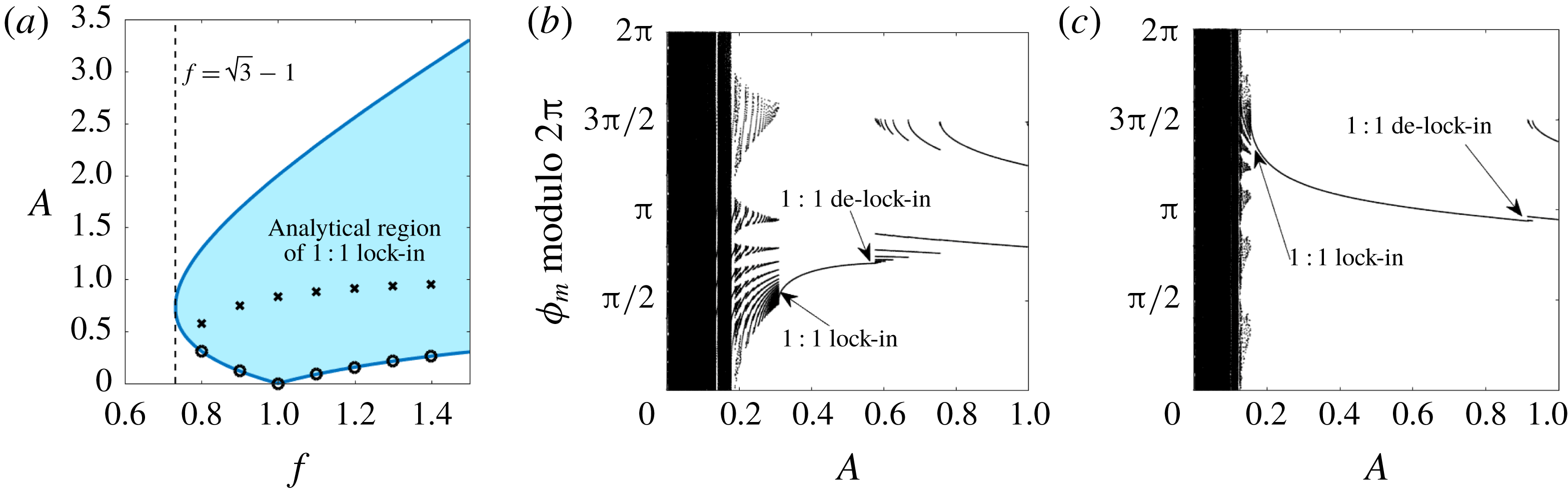
do not agree with the numerical results. This is illustrated through figure 9(a) for
 $1:1$
lock-in. The dark blue line in figure 9(a) represents the boundary of lock-in obtained through the analytical expression for
 $A_{min}$
and
 $A_{max}$
. The shaded region inside the boundary represents the lock-in state. Hollow circles and crosses respectively indicate the onset and end of the lock-in state obtained from the numerical simulations. It is observed that
 $A_{min}$
agrees exactly with the onset of lock-in, while the end of lock-in is highly over predicted by the analytical solution. The occurrence of de-lock-in at lower amplitudes is observed from the iterates (numerical simulations) of
 $\unicode[STIX]{x1D719}_{m}$
(modulo
 $2\unicode[STIX]{x03C0}$
) with respect to
 $A$
for
 $f=0.8$
(panel b) and
 $f=1.2$
(panel c).
To summarize, exact agreement occurs for the lower boundary of lock-in between the analytical solution and numerical simulations, while there is a disagreement in prediction of the onset of de-lock-in. We explore this discrepancy further using cobweb diagrams in the next section.
(a) Comparison between analytical and numerical results for lock-in boundary. Dark blue line indicates
 $1:1$
lock-in boundary obtained using (3.21)–(3.24), inside which (blue shaded region) lock-in is expected to occur. Circle and cross symbols represent the amplitude values obtained from numerical simulations at which lock-in and de-lock-in occurs respectively. Iterates of
 $\unicode[STIX]{x1D719}_{m}$
(modulo
 $2\unicode[STIX]{x03C0}$
) obtained numerically with
 $A$
as parameter and (b)
 $f=0.8$
, (c)
 $f=1.2$
.

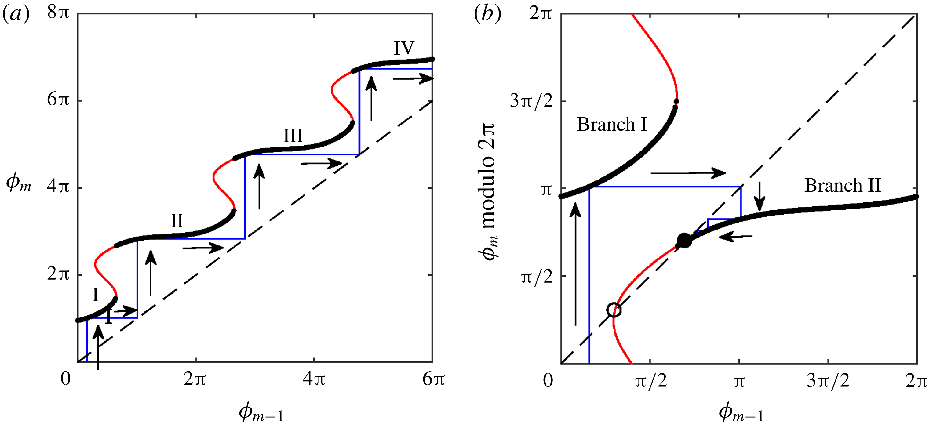
First return map of (2.11),
 $\unicode[STIX]{x1D719}_{m}-\unicode[STIX]{x1D719}_{m-1}$
, along with cobweb diagram (a) before and (b) after modulo
 $2\unicode[STIX]{x03C0}$
operation on
 $\unicode[STIX]{x1D719}_{m}$
. Dashed line indicate
 $\unicode[STIX]{x1D719}_{m}=\unicode[STIX]{x1D719}_{m-1}$
. The parameters are
 $f=0.8$
and
 $A=0.5$
, with the initial condition
 $\unicode[STIX]{x1D719}_{0}=0.5$
. The thick black curve shows the physically relevant first root
 $\unicode[STIX]{x1D719}_{m}$
of (2.11). This curve has discontinuities in
 $\unicode[STIX]{x1D719}_{m}$
and its piecewise continuous segments are marked as branches I, II and so on. The second and higher roots of
 $\unicode[STIX]{x1D719}_{m}$
are shown by thin red curves. Thin blue lines indicate the cobwebs. The direction of the arrow represents the evolution of the cobwebs. Only branches I and II appear after the modulo operation (panel b). The intersection of the first return map (panel b) with
 $\unicode[STIX]{x1D719}_{m}=\unicode[STIX]{x1D719}_{m-1}$
represents the fixed points associated with lock-in. Solid and hollow circles indicate linearly stable and unstable fixed points.

4 Investigation of 1 : 1 de-lock-in
The first return map of (2.11),
 $\unicode[STIX]{x1D719}_{m}-\unicode[STIX]{x1D719}_{m-1}$
, is shown in figure 10(a) for
 $f=0.8,A=0.5$
. As said earlier, for a given
 $\unicode[STIX]{x1D719}_{m-1}$
, the presence of harmonic terms in (2.11) leads to multiple solutions for
 $\unicode[STIX]{x1D719}_{m}$
. This is evident from the multivalued nature of the first return map. However, as discussed at the end of § 2.1, the physically relevant solution is the first root of
 $\unicode[STIX]{x1D719}_{m}$
. It is shown as a thick black curve in figure 10(a). As one traces the black curve, discontinuity in
 $\unicode[STIX]{x1D719}_{m}$
occurs. The piecewise continuous curve segments are identified as branch I, II and so on. Although the second and higher roots of
 $\unicode[STIX]{x1D719}_{m}$
are not physically relevant, they are plotted (thin red curves) in the first return map to explain the discrepancy between the analytical and numerical lock-in boundaries.
The dashed line indicates
 $\unicode[STIX]{x1D719}_{m}=\unicode[STIX]{x1D719}_{m-1}$
. A cobweb diagram (thin blue lines) is constructed to study the dynamics of the map, given an initial condition
 $\unicode[STIX]{x1D719}_{0}$
. From
 $\unicode[STIX]{x1D719}_{0}$
(set as 0.5 in figure 10
a), the successive iterates
 $\unicode[STIX]{x1D719}_{1},\unicode[STIX]{x1D719}_{2},\ldots$
are obtained by moving vertically and horizontally towards the first return map and the dashed line respectively. Cobwebs show that the iterates grow unboundedly. Since the iterates represent the phase points on the circle, a modulo
 $2\unicode[STIX]{x03C0}$
operation on
 $\unicode[STIX]{x1D719}_{m}$
bounds
 $\unicode[STIX]{x1D719}_{m-1}$
and
 $\unicode[STIX]{x1D719}_{m}$
to
 $[0,2\unicode[STIX]{x03C0}]$
. This helps the illustration of lock-in and de-lock-in processes elegantly. Figure 10(b) shows the corresponding return map and the cobweb diagram after the modulo operation (indicated as modulo
 $2\unicode[STIX]{x03C0}$
). Only branches I and II appear after the modulo operation. The parameters considered for figure 10 lie in the
 $1:1$
lock-in region. During lock-in,
 $\unicode[STIX]{x1D719}_{m}=\unicode[STIX]{x1D719}_{m-1}+2\unicode[STIX]{x03C0}$
. Therefore, after the modulo operation, we converge to a fixed point (black filled circle) in the
 $\unicode[STIX]{x1D719}_{m}(\text{modulo}~2\unicode[STIX]{x03C0})$
–
 $\unicode[STIX]{x1D719}_{m-1}$
plane (see figure 10
b), which corresponds to a period-1 solution in figure 10(a).
Cobweb diagrams and first return map of (2.11) for
 $f=0.8$
across various amplitudes: (a)
 $A=0.05$
, (b)
 $A_{min}=0.31$
, (c)
 $A=0.5$
, (d)
 $A_{de\text{-}lock}=0.58$
, (e)
 $A=0.9$
. Solid and hollow circles indicate linearly stable and unstable fixed points. The vertical and slanted dashed lines represent the location of the stable fixed point and
 $\unicode[STIX]{x1D719}_{m}=\unicode[STIX]{x1D719}_{m-1}$
respectively. Arrows show the flow of the map from
 $\unicode[STIX]{x1D719}_{0}$
. (f) Green shaded portion indicates the modified region of lock-in. The onset of lock-in and de-lock-in observed in the numerical simulations (figure 9
a) are indicated as circular and cross symbols respectively.

Figure 11 shows the evolution of the cobweb for increasing values of
 $A$
at
 $f=0.8$
. At the lowest amplitude (
 $A=0.05$
), the first return map does not intersect
 $\unicode[STIX]{x1D719}_{m}=\unicode[STIX]{x1D719}_{m-1}$
(panel a). The iterates of the map jump between branches I and II. On increasing the number of iterates, the cobwebs densely fill a region in the plane, indicating that the trajectory is quasi-periodic. On increasing
 $A$
to 0.5 (panel c), the map intersects
 $\unicode[STIX]{x1D719}_{m}=\unicode[STIX]{x1D719}_{m-1}$
at two locations, leading to the existence of
 $1:1$
lock-in fixed points. At one of the fixed points (marked as a hollow circle), the slope of the return map is more than one, indicating that it is linearly unstable. At the other fixed point (solid circle), the slope is less than one, identifying it as stable. These two fixed points are obtained exactly from our analytical investigation described in figure 7(b,d). The cobwebs converge to the stable fixed point leading to lock-in. The onset of lock-in is identified by the coalescence of these two fixed points, which occurs at
 $A=A_{min}=0.31$
(see panel b). The fixed points lie only on branch II. During lock-in (panels b,c), when the cobweb reaches branch II, it remains in branch II approaching the stable fixed point. When
 $A$
is increased to 0.9 (panel e), the fixed point, marked as a solid circle, still remains linearly stable. However, the cobweb alternates between branches I and II. This occurs because branch I protrudes to the right of the stable fixed point. This protrusion means that branch I contains the first root (
 $\unicode[STIX]{x1D719}_{m}$
) of (2.11). Therefore, a cobweb initially in branch II, as it approaches the stable fixed point jumps to branch I. This diverts the cobweb away from the fixed point and the cycle repeats. Based on the number of loops between branches I and II in the cobweb diagram, the period of the orbit can be determined. The presence of the stable fixed point is predicted from our analytical investigation. Although it exists, the cobwebs do not reach it. Hence, de-lock-in observed in the numerical simulations is not predicted from the analytical study.
The exact parameter location where de-lock-in occurs can be predicted from the geometry of the first return map. The cobweb diagram at the onset of de-lock-in is shown in figure 11(d) (
 $A=0.58$
). At the location of
 $\unicode[STIX]{x1D719}_{m-1}$
, where the stable fixed point is present, branch I just turns back on itself, leading to its slope becoming infinity. Mathematically, this becomes
 $$\begin{eqnarray}\left.\frac{\text{d}\unicode[STIX]{x1D719}_{m}}{\text{d}\unicode[STIX]{x1D719}_{(m-1)}}\right|_{A_{de\text{-}lock}}=\left.\frac{-\unicode[STIX]{x2202}F/\unicode[STIX]{x2202}\unicode[STIX]{x1D719}_{m-1}}{\unicode[STIX]{x2202}F/\unicode[STIX]{x2202}\unicode[STIX]{x1D719}_{m}}\right|_{A_{de\text{-}lock}}=\infty ,\end{eqnarray}$$
where
 $A_{de\text{-}lock}$
represents the critical amplitude at the onset of de-lock-in. The above equation translates to
 $\unicode[STIX]{x2202}F/\unicode[STIX]{x2202}\unicode[STIX]{x1D719}_{m}|_{A_{de\text{-}lock}}=0$
. From appendix B, the expression for
 $\unicode[STIX]{x2202}F/\unicode[STIX]{x2202}\unicode[STIX]{x1D719}_{m}$
can be obtained. The condition now becomes
 $$\begin{eqnarray}-\left(\frac{A_{de\text{-}lock}^{2}}{4}+\frac{1}{2}\right)+\unicode[STIX]{x03C0}fA_{de\text{-}lock}\cos \unicode[STIX]{x1D719}_{m}+\frac{A_{de\text{-}lock}^{2}}{4}\cos 2\unicode[STIX]{x1D719}_{m}-A_{de\text{-}lock}\sin \unicode[STIX]{x1D719}_{m}=0.\end{eqnarray}$$
In the above equation, for a given
 $f$
, there are two unknowns
 $\unicode[STIX]{x1D719}_{m},A_{de\text{-}lock}$
. Another equation is required for the closure, which is obtained as follows. At the onset of de-lock-in,
 $\unicode[STIX]{x1D719}_{m-1}$
is same as the analytical solution for
 $\unicode[STIX]{x1D719}_{m-1,2}$
, which is a function of
 $A_{de\text{-}lock}$
:
 $$\begin{eqnarray}\unicode[STIX]{x1D719}_{m-1}=\unicode[STIX]{x1D719}_{m-1,2}=\unicode[STIX]{x03C0}-\arcsin \left(\frac{[A_{de\text{-}lock}^{2}+2(1-f)]}{2A_{de\text{-}lock}f}\right).\end{eqnarray}$$
Using this
 $\unicode[STIX]{x1D719}_{m-1}$
, the value of
 $\unicode[STIX]{x1D719}_{m}$
is obtained by numerically solving the map equation (2.11):
 $$\begin{eqnarray}\displaystyle & & \displaystyle (\unicode[STIX]{x1D719}_{m-1,2}-\unicode[STIX]{x1D719}_{m})\left(\frac{A_{de\text{-}lock}^{2}}{4}+\frac{1}{2}\right)+\unicode[STIX]{x03C0}f(A_{de\text{-}lock}\sin \unicode[STIX]{x1D719}_{m}+1)\nonumber\\ \displaystyle & & \displaystyle \quad +\,\frac{A_{de\text{-}lock}^{2}}{8}(\sin 2\unicode[STIX]{x1D719}_{m}-\sin 2\unicode[STIX]{x1D719}_{m-1,2})+A_{de\text{-}lock}(\cos \unicode[STIX]{x1D719}_{m}-\cos \unicode[STIX]{x1D719}_{m-1,2})=0.\end{eqnarray}$$
The unknowns
 $A_{de\text{-}lock},\unicode[STIX]{x1D719}_{m-1,2},\unicode[STIX]{x1D719}_{m}$
are obtained by solving numerically the simultaneous nonlinear equations (4.2)–(4.4). The value of
 $A_{de\text{-}lock}$
extracted in this way matches exactly with our numerical simulations. The boundary of de-lock-in is plotted as a black line in figure 11(f). The green shaded portion indicates the modified region of lock-in.
4.1 Extension to
$p:1$
de-lock-in:

The use of cobweb diagrams can be extended to study higher-order lock-in and de-lock-in behaviour. Figure 12 illustrates the evolution of the map through cobweb diagrams for
 $f=1.8$
, as one increases
 $A$
. The iterates
 $\unicode[STIX]{x1D719}_{m}$
are plotted in panel (a) indicating the nature of the map at various values of
 $A$
. For the lowest value of
 $A=A_{1}=0.05$
, the first return map does not intersect
 $\unicode[STIX]{x1D719}_{m}=\unicode[STIX]{x1D719}_{m-1}$
leading to the absence of lock-in state (see panel b). The cobwebs jump between the two branches of the first return map. The geometry of the cobwebs indicates a quasi-periodic solution, which can also be seen from the iterates densely filling the space at
 $A_{1}$
in panel (a). As one increases the amplitude to
 $A=A_{2}=0.12$
, branch II (the word ‘branch’ is omitted in the panels) of the first return map touches
 $\unicode[STIX]{x1D719}_{m}=\unicode[STIX]{x1D719}_{m-1}$
indicating the onset of lock-in (see panel c). At this point,
 $\unicode[STIX]{x1D719}_{m-1}=\unicode[STIX]{x03C0}/2$
. The map equation (2.11) is then solved to obtain
 $\unicode[STIX]{x1D719}_{m}$
and the instantaneous vortex shedding time period,
 $\unicode[STIX]{x0394}t_{m}$
, is calculated to be 1.11. Hence
 $f/(1/\unicode[STIX]{x0394}t_{m})=1.8/(1/1.1)=2$
, indicating a
 $2:1$
lock-in. Further increasing
 $A$
to
 $A_{3}=0.2$
, two
 $2:1$
lock-in fixed points (one linearly stable and other unstable) appear (panel d). Cobwebs converge to the stable fixed point present in branch II. When the amplitude reaches
 $A=A_{4}=0.26$
, branch I touches the abscissa of the stable fixed point, leading to the onset of de-lock-in (panel e). Between amplitudes
 $A_{2}$
and
 $A_{4}$
,
 $2:1$
lock-in occurs (identified as a single curve in panel a). For higher amplitudes,
 $A=A_{5}=0.36$
, branch I protrudes to the right of the stable fixed point, leading to the cobwebs alternating between branches I and II (panel f). As in the previous case (see the first part of § 4), although a stable fixed point exists, the cobwebs never reach it and therefore lock-in does not occur. Further increase of
 $A$
to
 $A_{6}=0.40$
leads to the third intersection of the first return map with
 $\unicode[STIX]{x1D719}_{m}=\unicode[STIX]{x1D719}_{m-1}$
(panel g). This time, the new lock-in solution is born on branch I. At this point
 $\unicode[STIX]{x1D719}_{m-1}=3\unicode[STIX]{x03C0}/2$
and using (2.11),
 $\unicode[STIX]{x1D719}_{m}$
is found and eventually
 $\unicode[STIX]{x0394}t_{m}$
is evaluated to be 0.55. This indicates
 $f/(1/\unicode[STIX]{x0394}t_{m})=1.8/(1/0.55)=1$
, meaning the onset of
 $1:1$
lock-in. The iterates (panel a) show the presence of higher-periodic solutions between
 $A_{4}$
and
 $A_{6}$
. Above the amplitude
 $A_{6}$
, the third solution splits into a stable and unstable fixed point associated with
 $1:1$
lock-in (panel h for
 $A=A_{7}=0.5$
). Cobwebs converge to the stable fixed point in branch I. Note that at
 $A_{7}$
(panel h), a new branch III appears from the left, while the solution in branch II ceases to be the first root of
 $\unicode[STIX]{x1D719}_{m}$
.
(a) The iterates of
 $\unicode[STIX]{x1D719}_{m}$
(modulo
 $2\unicode[STIX]{x03C0}$
) for
 $f=1.8$
across various amplitudes. Cobweb diagram and first return map of (2.11) for (b)
 $A=A_{1}=0.05$
, (c)
 $A=A_{2}=0.12$
, (d)
 $A=A_{3}=0.2$
, (e)
 $A=A_{4}=0.26$
, (f)
 $A=A_{5}=0.36$
, (g)
 $A=A_{6}=0.40$
, (h)
 $A=A_{7}=0.5$
, (i)
 $A=A_{8}=0.98$
, (j)
 $A=A_{9}=0.99$
. Solid and hollow circles indicate linearly stable and unstable fixed points respectively. Vertical and slanted dashed lines represent the location of the stable fixed point and
 $\unicode[STIX]{x1D719}_{m}=\unicode[STIX]{x1D719}_{m-1}$
respectively. Arrows show the flow of the map from
 $\unicode[STIX]{x1D719}_{0}$
. I, II and III indicate branches I, II and III respectively

(a) Iterates of the instantaneous vortex shedding time period
 $\unicode[STIX]{x0394}t_{m}$
for various forcing amplitudes
 $A$
at frequency
 $f=3.2$
. Regions where the iterates form a horizontal line represent
 $3:1,2:1,1:1$
lock-in. (b) Colour shaded regions represent
 $1:1$
(green),
 $2:1$
(pink),
 $3:1$
(blue) lock-in states. Vertical dashed line indicates the location,
 $f=3.2$
. Arrow indicates the direction of increasing
 $A$
.

Amplitude
 $A=A_{8}=0.98$
(panel i) lies at the onset of
 $1:1$
de-lock-in. At this amplitude, branch III touches the abscissa of the stable fixed point (on branch I) that formed the solution of
 $1:1$
lock-in. As before, although the cobwebs tend to approach the stable fixed-point, they are diverted away by the protrusion of branch III. Higher-periodic solutions (in this case two period) appear beyond
 $A_{8}$
(see the iterates in panel a). In conclusion, we observe that when the system is forced away from the steady-state vortex shedding frequency, for sufficiently high amplitudes, it locks in to the nearest
 $p:1$
state. As the amplitude is increased further, de-lock-in occurs and then the system moves on to lock-in the
 $(p-1):1$
state. This process continues till it reaches
 $1:1$
lock-in.
The critical amplitudes
 $A_{2}$
and
 $A_{6}$
are calculated from the analytical expression for
 $A_{min}$
, given by (3.21) and (3.23) respectively.
 $A_{2}$
and
 $A_{6}$
are associated with the onset of
 $2:1$
and
 $1:1$
lock-in and hence the expression for
 $A_{min}$
associated with
 $f/p=1.8/2<1$
and
 $f/p=1.8/1>1$
is used respectively. The amplitude
 $A_{8}$
where
 $1:1$
de-lock-in occurs is obtained by solving simultaneously (4.2)–(4.4), as described in the fist part of § 4. To calculate
 $A_{4}$
(onset of
 $2:1$
de-lock-in), the same procedure is followed, by replacing
 $f$
with
 $f/2$
in (4.3). In general, to obtain the amplitude at which a
 $p:1$
de-lock-in occurs,
 $f/p$
is used in (4.3). We now focus on addressing the third observation recorded at the end of § 2.2. The numerical simulation shown in figure 6(e), where the system is forced at
 $f=3.2$
, is revisited. The iterates in terms of instantaneous vortex shedding time period
 $\unicode[STIX]{x0394}t_{m}$
are replotted in figure 13(a) for clarity. At low amplitudes, the system reaches the
 $3:1$
lock-in state, followed by subsequent de-lock-in and lock-in processes to culminate ultimately in the
 $1:1$
lock-in state. Using the procedure described in the previous paragraph, the region of lock-in is obtained and shown for
 $1:1$
(green),
 $2:1$
(pink),
 $3:1$
(blue) states in figure 13(b). For
 $f=3.2$
(shown as a vertical dashed line), as one increases
 $A$
, the region of
 $3:1$
lock-in first appears followed by the
 $2:1$
and ending up in the
 $1:1$
state. The current paper not only shows the existence of de-lock-in with higher amplitudes, but also the shift from one lock-in state to another. These predictions are open for experimental verification.
Comparisons made between the predictions of the map and the existing experimental results. Panels (a) and (c) compare the mean of instantaneous vortex shedding frequency for various excitation frequencies at a given amplitude (
 $A=0.071$
and
 $0.08$
for (a) and (c) respectively). Panels (b) and (d) compare
 $1:1$
and
 $2:1$
lock-in boundaries respectively with the map. Our comparisons are made with four geometrical experimental configurations. Panels (a,b) correspond to the results of vortex shedding behind an annular ring, and a triangular bluff body is used in panel (c). In panel (d) square and cross symbols indicate configurations of a rectangular bluff body and flat plate respectively.

In the past, de-lock-in was observed extensively in various biological (Guevara, Glass & Shrier Reference Guevara, Glass and Shrier1981, Guevara & Glass Reference Guevara and Glass1982) and physical systems (convective flow, hydrodynamic instabilities: Gollub & Benson Reference Gollub and Benson1980, Marques, Lopez & Shen Reference Marques, Lopez and Shen2001). However, in the context of externally excited thermoacoustic interactions, de-lock-in was recently reported in Guan, Murugesan & Li (Reference Guan, Murugesan and Li2018), which contained a wealth of information. Original theoretical investigations were performed by Aronson et al. (Reference Aronson, Chory, Hall and McGehee1982), Afraimovich & Shilnikov (Reference Afraimovich and Shilnikov1991) and the results were compiled in textbooks Pikovsky et al. (Reference Pikovsky, Rosenblum and Kurths2003), Balanov et al. (Reference Balanov, Janson, Postnov and Sosnovtseva2008) and Arnold et al. (Reference Arnold, Afrajmovich, Il’yashenko and Shil’nikov2013). In particular, the papers Anishchenko, Safonova & Chua (Reference Anishchenko, Safonova and Chua1993) and Guan et al. (Reference Guan, Murugesan and Li2018) described three routes to de-lock-in that can occur from a lock-in state in a periodically forced oscillator. The routes are given as follows. Route I: stable period-1 fixed point (lock-in state) disappears through a series of period-doubling bifurcations. Route II: stable and unstable period-1 fixed points merge to form a saddle-node bifurcation. Route III: stable and unstable manifolds of the period-1 fixed point become tangent to each other, forming a homoclinic orbit. In the present case, the iterates shown in figure 9(b,c) do not show period-doubling bifurcation at de-lock-in. Furthermore, the stable and unstable period-1 fixed points continue to exist at de-lock-in (see figures 11 d and 12 e,i). Therefore, routes I and II do not occur in the current paper. This indicates the possibility of the presence of route III. However, in order to confirm, calculation/computation of the stable and unstable manifolds is required. The authors believe that this could be a separate investigation, which could be taken up in the future.
5 Comparison with experiments
In this section, we compare our analytical predictions with the available experimental results in the literature, pertaining to lock-in. This comparison allows one to identify the strength and weakness of the lower-order model used. The comparison is first made with the results for non-reacting flows (Al-Asmi & Castro Reference Al-Asmi and Castro1992; Castro Reference Castro1997) and then extended to reacting flow configurations (Li & Juniper Reference Li and Juniper2013b ).
Castro (Reference Castro1997) investigated the response in terms of instantaneous vortex shedding frequency (
 $1/\unicode[STIX]{x0394}t_{m}$
) behind an annular ring under upstream velocity excitation. For a range of excitation frequency,
 $1/\unicode[STIX]{x0394}t_{m}$
from the experiments (hollow circles) is compared with the iterates of the map at
 $A=0.071$
(figure 14
a). The lock-in region (
 $1:1$
in this figure) of the map is indicated in a grey shade. In the region where lock-in is absent, the mean of the map iterates (blue continuous curve) is compared with the experimental results. Although the region of lock-in is over-predicted by the map, the qualitative trend in the (mean) instantaneous vortex shedding frequency is portrayed by the lower-order model. Furthermore, the onset of lock-in for
 $f<1$
is quantitatively well predicted. This observation holds true for other amplitudes, as shown in figure 14(b). On the other hand, the onset in
 $f>1$
is not well captured by the map. Higher-order
 $(2:1)$
lock-in in various other geometries was reported by Al-Asmi & Castro (Reference Al-Asmi and Castro1992). Figure 14(c) compares (mean)
 $1/\unicode[STIX]{x0394}t_{m}$
between the map and experimental investigations conducted on a triangular bluff body at
 $A=0.08$
. Contrary to the previous case (figure 14
a,b), lock-in regions (both
 $1:1$
and
 $2:1$
) are under-predicted. A good match (especially the boundary associated with
 $f<2$
) in the
 $2:1$
lock-in boundary is observed for the case of a rectangular bluff body (open square symbol in figure 14
d). The match deteriorates when the rectangular body is replaced by a flat plate (cross symbol in figure 14
d). To summarize, the experimental results of Castro (Reference Castro1997) and Al-Asmi & Castro (Reference Al-Asmi and Castro1992) indicate that lock-in boundaries strongly depend on the geometry of the bluff body. The current map appears to predict closely the boundary associated with the rectangular bluff body. On the whole, the qualitative trend in the vortex shedding frequency observed in the experiments is captured well by the model.
Comparison of the lock-in boundary predicted from the map and measured experimentally Li & Juniper (Reference Li and Juniper2013b ) for a hydrodynamically self-excited diffusion flame. Lock-in boundaries for two fuel (methane) concentrations (blue and red curves), compared with that of the map (black curve). Shaded region indicate lock-in state. Panels (a) and (b) correspond to the presence and absence of coflow air respectively.

In reacting flows, Li & Juniper (Reference Li and Juniper2013b
) experimentally reported
 $1:1$
lock-in on a hydrodynamically self-excited jet diffusion flame configuration (figure 15). The flame was stabilized in a coaxial injector with methane/nitrogen mixture as fuel. Two configurations, in the presence and absence of coflow air, for various proportions of the methane/nitrogen mixture were investigated. For the case of coflow (figure 15
a), a good match is observed in the lock-in boundary near
 $f>1$
. Moreover, the asymmetry in the boundary is qualitatively captured by the model. On the left-hand part of the boundary (
 $f<1$
), the frequency (
 $f=0.75$
for 60 % and
 $f=0.78$
for 100 % concentration of methane) associated with the large amplitude required for lock-in is close to
 $f_{min}$
(below which lock-in does not occur in the lower-order model). The quantitative match deteriorates when one compares with the no-coflow configuration (figure 15
b). Although the lower-order model used was developed for non-reacting flows, it provides a good qualitative illustration for the dynamics of lock-in experimentally observed both in non-reacting and reacting flows. The model however has a weakness, as it cannot predict the difference in lock-in behaviour arising from various bluff body configurations and flame characteristics. The shape of the lock-in boundary in the model is primarily determined by (2.1) describing the time evaluation of
 $\unicode[STIX]{x1D6E4}_{m}$
. To obtain a better match, the following is proposed. Using time-resolved velocity measurements near a given bluff body,
 $\unicode[STIX]{x1D6E4}_{m}$
is calculated. The measured
 $\unicode[STIX]{x1D6E4}_{m}$
is fitted to an equation having a functional dependence on the excitation velocity (similar to (2.1)). Then, the analytical procedure described in the paper can be performed to obtain the region of lock-in. This method is proposed in principle and the implementation details can be taken up as a separate investigation.
6 Conclusion
An analytical investigation is performed to understand the unsteady dynamics of vortex shedding behind the flame holder of combustors under upstream forced harmonic excitation. Of the observed various dynamical features, the paper is focused on studying the phenomenon of lock-in. As combustion instability is accompanied by lock-in, understanding the various features of lock-in is of practical relevance. During lock-in, vortex shedding occurs at the forcing frequency. We begin with the lower-order model given in Matveev & Culick (Reference Matveev and Culick2003), which describes the dynamics response of the vortex shedding process to any upstream velocity fluctuations. The continuous time domain model is converted to a map, which relates the current and previous shedding time instances. The map is implicit and nonlinear. Frequency ratio (ratio of forcing to natural vortex shedding frequency) and amplitude of the excitation velocity are the two governing parameters which are varied. The instantaneous time period of vortex shedding is monitored as the response of the system. Initially numerical simulation of the map is performed to extract the iterates. In the absence of forcing, the iterates of the map indicates that shedding occurs at the natural vortex shedding frequency. As the amplitude is increased, the iterates display quasi-periodic behaviour. Beyond a threshold amplitude, the iterates present a period-1 fixed point indicating a lock-in state. In general, we observed
 $p:1$
lock-in, where the ratio of forcing to the vortex shedding frequency is
 $p$
. Further above a critical amplitude, the period-1 fixed point disappears, leading to de-lock-in. The amplitude at which lock-in and de-lock-in occurs strongly depends on the frequency ratio.
For analytical manipulation, the time instances of vortex shedding are mapped to phase points on a circle. The map equation is transformed, so that it relates the phase points of current and previous vortex shedding time instances. After applying the condition for
 $p:1$
lock-in, the map equation becomes an analytical relation between frequency ratio and amplitude to be satisfied during lock-in. From the algebraic nature of the relation, the following conclusions can be made. (1) A
 $p:1$
lock-in does not occur if the frequency ratio is less than
 $f_{min}=p(\sqrt{3}-1)$
for any amplitude. (2) At the onset of lock-in, two period-1 solutions appear with one (linearly) stable and the other unstable, leading to the occurrence of a saddle-node bifurcation. (3) The boundary of the onset of
 $p:1$
lock-in shows that lock-in occurs at a lower amplitude when the frequency ratio is closer to
 $p$
. The boundary is asymmetric with respect to the frequency ratio
 $p$
. Lock-in occurs at lower amplitudes on the side where the frequency ratio is greater than
 $p$
: an observation experimentally reported by Li & Juniper (Reference Li and Juniper2013b
). However, the amplitude where de-lock-in occurs (from the numerical simulation) is over-predicted by the analytical relation. The discrepancy is explained through cobweb diagrams between the phase points of the map, plotted for various amplitudes at a given frequency ratio. In the cobweb diagram, we observe that the first return map contains two branches and the stable lock-in fixed point exist on one of the branches. At the onset of de-lock-in, the other branch just touches the phase point associated with the stable fixed point and moves to the right at higher amplitudes. This geometrical feature of the first return map diverts the iterates away from the stable fixed point. Although the stable lock-in solution exists, the iterates never reach it causing de-lock-in. Based on the geometry of the first return map, the exact threshold where de-lock-in begins can be calculated.
On the whole, boundaries for
 $1:1,2:1,\ldots ,p:1$
lock-in regions can be plotted in the parameter space of frequency ratio and amplitude. Although the numerical value of
 $f_{min}$
is specific to the current model, we believe that such a cut-off frequency might be present in a practical combustor. Together, the shape of the lock-in boundary and the cut-off frequency provide engineers with a priori information about the possible regions of lock-in. In the end, from the lock-in boundary, we observe that when the system is forced near the harmonics of the natural vortex shedding frequency, vortices are locked to the nearest
 $p:1$
state. Upon increasing the forcing amplitude, de-lock-in occurs and is followed by the next lower-order lock-in
 $p-1:1$
state. This process repeats till the system reaches the
 $1:1$
state. This prediction is yet to be verified through experiments.
Acknowledgements
The authors are grateful to Professors A. Chatterjee, M. Banerjee and P. Wahi, Indian Institute of Technology Kanpur for their insightful comments and suggestions during the course of this investigation.
Plot of
 $F(\unicode[STIX]{x1D719}_{m})$
with respect to
 $\unicode[STIX]{x1D719}_{m}$
for (a)
 $f=0.8,A=0,\unicode[STIX]{x1D719}_{m-1}=0$
, (b)
 $f=0.8,A=0.05,\unicode[STIX]{x1D719}_{m-1}=0$
and (c)
 $f=0.8,A=0.5({>}A_{th}),\unicode[STIX]{x1D719}_{m-1}=1.5$
. The boundaries of the sub-intervals are shown by short vertical lines. Circle symbol indicates the required root. (d) Plot of
 $\text{d}F/\text{d}\unicode[STIX]{x1D719}_{m}$
with
 $\unicode[STIX]{x1D719}_{m}$
for
 $A=0,0.05,A_{th}=0.20$
.

Appendix A.
The implicit map (2.11) can be represented in the following form:
 $F(\unicode[STIX]{x1D719}_{m},\unicode[STIX]{x1D719}_{m-1},A,f)=0$
. For a given value of
 $A,f$
and
 $\unicode[STIX]{x1D719}_{m-1}$
, it is required to find the first root
 $\unicode[STIX]{x1D719}_{m}$
for which the curve
 $F=0$
. The technique to compute
 $\unicode[STIX]{x1D719}_{m}$
from this nonlinear implicit equation follows two algorithms. We use the following to illustrate its need. For
 $f=0.8,A=0,\unicode[STIX]{x1D719}_{m-1}=0$
, the plot of
 $F(\unicode[STIX]{x1D719}_{m})$
with
 $\unicode[STIX]{x1D719}_{m}$
is shown in figure 16(a). We observe that
 $F(\unicode[STIX]{x1D719}_{m})$
is monotonic and therefore becomes zero only once. This forms the unique root for
 $F(\unicode[STIX]{x1D719}_{m})=0$
. The curve
 $F(\unicode[STIX]{x1D719}_{m})$
still remains monotonic for a slightly higher amplitude,
 $A=0.05$
(figure 16
b). For a larger amplitude
 $A=0.5$
and
 $f=0.8,\unicode[STIX]{x1D719}_{m-1}=1.5$
,
 $F(\unicode[STIX]{x1D719}_{m})$
becomes non-monotonic with zero crossings occurring at three locations. The required solution
 $\unicode[STIX]{x1D719}_{m}$
is the first instance when
 $F(\unicode[STIX]{x1D719}_{m})=0$
. The first algorithm is relatively simple and it is designed to find the unique root (figure 16
a,b). On the other hand, the second algorithm involves multiple steps to identify the first root (figure 16
c). The need to use a particular algorithm depends on the existence of
 $\text{d}F/\text{d}\unicode[STIX]{x1D719}_{m}=0$
for any
 $\unicode[STIX]{x1D719}_{m}$
. The required equation is
 $$\begin{eqnarray}\frac{\text{d}F}{\text{d}\unicode[STIX]{x1D719}_{m}}=-\left(\frac{A^{2}}{4}+\frac{1}{2}\right)+\unicode[STIX]{x03C0}fA\cos \unicode[STIX]{x1D719}_{m}+\frac{A^{2}}{4}\cos 2\unicode[STIX]{x1D719}_{m}-A\sin \unicode[STIX]{x1D719}_{m}=0.\end{eqnarray}$$
The above equation is harmonic with respect to
 $\unicode[STIX]{x1D719}_{m}$
as shown in figure 16(d). For
 $A=0$
,
 $\text{d}F/\text{d}\unicode[STIX]{x1D719}_{m}=-0.5$
, indicating a straight line for
 $F(\unicode[STIX]{x1D719}_{m})$
. As the value of
 $A$
is increased, the harmonic terms begin to dominate. At a certain amplitude (
 $A=A_{th}$
), we observe that
 $\text{d}F/\text{d}\unicode[STIX]{x1D719}_{m}$
touches zero. This occurs when
 $\unicode[STIX]{x1D719}_{m}\approx 2\unicode[STIX]{x03C0}$
. Therefore, we substitute
 $\unicode[STIX]{x1D719}_{m}=2\unicode[STIX]{x03C0}$
in (A 1) to obtain an approximate estimate for
 $A_{th}$
,
 $$\begin{eqnarray}A_{th}\approx \frac{1}{2\unicode[STIX]{x03C0}f}.\end{eqnarray}$$
Algorithms 1 and 2 are chosen when
 $A\leqslant A_{th}$
and
 $A\geqslant A_{th}$
respectively for a given
 $f$
. Note that the above method of choosing an algorithm is independent of
 $\unicode[STIX]{x1D719}_{m-1}$
.
A.1 Algorithm 1
Since, algorithm 1 is applied for low amplitudes, the linear terms (in
 $\unicode[STIX]{x1D719}_{m}$
) dominate over the nonlinear (harmonic) terms. The linear part (
 $y(\unicode[STIX]{x1D719}_{m})$
) of
 $F(\unicode[STIX]{x1D719}_{m})=0$
(2.11) is
 $$\begin{eqnarray}y(\unicode[STIX]{x1D719}_{m})=-\unicode[STIX]{x1D719}_{m}\left(\frac{A^{2}}{4}+\frac{1}{2}\right)+\unicode[STIX]{x1D719}_{m-1}\left(\frac{A^{2}}{4}+\frac{1}{2}\right)-\frac{A^{2}}{8}\sin 2\unicode[STIX]{x1D719}_{m-1}-A\cos \unicode[STIX]{x1D719}_{m-1}+\unicode[STIX]{x03C0}f.\end{eqnarray}$$
The root
 $(\unicode[STIX]{x1D719}_{cr})$
of the above equation
 $y=0$
is
 $$\begin{eqnarray}\unicode[STIX]{x1D719}_{cr}=\frac{\displaystyle \left[\unicode[STIX]{x1D719}_{m-1}\left(\frac{A^{2}}{4}+\frac{1}{2}\right)-\frac{A^{2}}{8}\sin 2\unicode[STIX]{x1D719}_{m-1}-A\cos \unicode[STIX]{x1D719}_{m-1}+\unicode[STIX]{x03C0}f\right]}{\displaystyle \left(\frac{A^{2}}{4}+\frac{1}{2}\right)}.\end{eqnarray}$$
The solution of the nonlinear map (2.11) lies near this root
 $\unicode[STIX]{x1D719}_{cr}$
. Hence, a bisection method is used by choosing an initial interval for the root
 $\unicode[STIX]{x1D719}_{m}$
to lie in
 $[0,(\unicode[STIX]{x1D719}_{cr}+2\unicode[STIX]{x03C0})]$
. It is found from our numerical simulations that the above interval is sufficient to capture the root.
A.2 Algorithm 2
The second algorithm used for
 $A>A_{th}$
is adapted from Kalmár-Nagy, Wahi & Halder (Reference Kalmár-Nagy, Wahi and Halder2011). That paper suggests dividing the curve
 $F(\unicode[STIX]{x1D719}_{m})$
into a number of sub intervals. The boundaries of the intervals are identified as where
 $\text{d}F/\text{d}\unicode[STIX]{x1D719}_{m}$
and
 $\text{d}^{2}F/\text{d}\unicode[STIX]{x1D719}_{m}^{2}$
vanish to zero. A number of such sub-intervals are shown in figure 16(c) (
 $f=0.8,A=0.5>A_{th}$
). In each sub-interval taken in the ascending order of
 $\unicode[STIX]{x1D719}_{m}$
, the bisection method is applied. The sub-interval where the root is first discovered is the required root. The equation to obtain a sub-interval is
 $$\begin{eqnarray}\displaystyle & \displaystyle \frac{\text{d}F}{\text{d}\unicode[STIX]{x1D719}_{m}}=-\left(\frac{A^{2}}{4}+\frac{1}{2}\right)+\unicode[STIX]{x03C0}fA\cos \unicode[STIX]{x1D719}_{m}+\frac{A^{2}}{4}\cos 2\unicode[STIX]{x1D719}_{m}-A\sin \unicode[STIX]{x1D719}_{m}=0, & \displaystyle\end{eqnarray}$$
 $$\begin{eqnarray}\displaystyle & \displaystyle \frac{\text{d}^{2}F}{\text{d}\unicode[STIX]{x1D719}_{m}^{2}}=-\unicode[STIX]{x03C0}fA\sin \unicode[STIX]{x1D719}_{m}-\frac{A^{2}}{2}\sin 2\unicode[STIX]{x1D719}_{m}-A\cos \unicode[STIX]{x1D719}_{m}=0. & \displaystyle\end{eqnarray}$$
Since (A 5)–(A 6) are
 $2\unicode[STIX]{x03C0}$
periodic, we first search for the sub-intervals in
 $\unicode[STIX]{x1D719}_{m}=[0,2\unicode[STIX]{x03C0}]$
. Inside
 $[0,2\unicode[STIX]{x03C0}]$
,
 $\text{d}F/\text{d}\unicode[STIX]{x1D719}_{m}$
and
 $\text{d}^{2}F/\text{d}\unicode[STIX]{x1D719}_{m}^{2}$
become zero at two locations. This can be explained as follows. Since we restrict our investigations to
 $A\leqslant 1$
, the terms with
 $A^{2}$
are less dominant in comparison to the terms with
 $A$
. The second-harmonic terms
 $(\sin 2\unicode[STIX]{x1D719}_{m},\cos 2\unicode[STIX]{x1D719}_{m})$
are associated with
 $A^{2}$
and make less contribution to
 $\text{d}F/\text{d}\unicode[STIX]{x1D719}_{m}$
and
 $\text{d}^{2}F/\text{d}\unicode[STIX]{x1D719}_{m}^{2}$
. Therefore (A 5)–(A 6) vary approximately at its fundamental frequency, leading to zero crossings only at two locations. This is evident from figure 17, where
 $\text{d}F/\text{d}\unicode[STIX]{x1D719}_{m}$
(solid blue curve) and
 $\text{d}^{2}F/\text{d}\unicode[STIX]{x1D719}_{m}^{2}$
(dotted green curve) are plotted for
 $f=0.8$
at
 $A=0.5$
(panel a) and
 $A=1$
(panel b). The exact locations (where
 $\text{d}F/\text{d}\unicode[STIX]{x1D719}_{m}=\text{d}^{2}F/\text{d}\unicode[STIX]{x1D719}_{m}^{2}=0$
) are identified by applying the bisection method, where the intervals are
 $[0,\unicode[STIX]{x03C0}/2],[\unicode[STIX]{x03C0}/2,\unicode[STIX]{x03C0}],[\unicode[STIX]{x03C0},3\unicode[STIX]{x03C0}/2],[3\unicode[STIX]{x03C0}/2,2\unicode[STIX]{x03C0}]$
. By this exercise, we obtain in total four sub-intervals (marked in figure 17
a). These sub-intervals are then used to extract the required root of
 $F(\unicode[STIX]{x1D719}_{m})=0$
. If the solution is absent inside
 $\unicode[STIX]{x1D719}_{m}=[0,2\unicode[STIX]{x03C0}]$
, the next four sub-intervals are identified by shifting the previous sub-intervals by
 $2\unicode[STIX]{x03C0}$
.
Plot of first and second derivatives of
 $F$
with respect to
 $\unicode[STIX]{x1D719}_{m}$
for
 $f=0.8$
at (a)
 $A=0.5$
and (b)
 $A=1$
. The four sub-intervals where
 $\text{d}F/\text{d}\unicode[STIX]{x1D719}_{m}=0$
and
 $\text{d}^{2}F/\text{d}\unicode[STIX]{x1D719}_{m}^{2}=0$
are marked.

Appendix B.
Implicit map (2.11) is of the form
 $F(\unicode[STIX]{x1D719}_{m},\unicode[STIX]{x1D719}_{m-1})=0$
. We have
 $$\begin{eqnarray}\left.\begin{array}{@{}c@{}}\displaystyle \frac{\text{d}}{\text{d}\unicode[STIX]{x1D719}_{m-1}}F(\unicode[STIX]{x1D719}_{m},\unicode[STIX]{x1D719}_{m-1})=\frac{\unicode[STIX]{x2202}F}{\unicode[STIX]{x2202}\unicode[STIX]{x1D719}_{m-1}}+\frac{\unicode[STIX]{x2202}F}{\unicode[STIX]{x2202}\unicode[STIX]{x1D719}_{m}}\frac{\text{d}\unicode[STIX]{x1D719}_{m}}{\text{d}\unicode[STIX]{x1D719}_{m-1}}=0\\ \displaystyle \;\Longrightarrow \;g^{\prime }=\frac{\text{d}\unicode[STIX]{x1D719}_{m}}{\text{d}\unicode[STIX]{x1D719}_{m-1}}=\frac{-\unicode[STIX]{x2202}F/\unicode[STIX]{x2202}\unicode[STIX]{x1D719}_{m-1}}{\unicode[STIX]{x2202}F/\unicode[STIX]{x2202}\unicode[STIX]{x1D719}_{m}}.\end{array}\right\}\end{eqnarray}$$
The numerator and denominator are obtained from the partial derivatives of (2.11),
 $$\begin{eqnarray}\displaystyle & \displaystyle \frac{\unicode[STIX]{x2202}F}{\unicode[STIX]{x2202}\unicode[STIX]{x1D719}_{m-1}}=\left(\frac{A^{2}}{4}+\frac{1}{2}\right)-\frac{A^{2}}{4}\cos 2\unicode[STIX]{x1D719}_{m-1}+A\sin \unicode[STIX]{x1D719}_{m-1}, & \displaystyle\end{eqnarray}$$
 $$\begin{eqnarray}\displaystyle & \displaystyle \frac{\unicode[STIX]{x2202}F}{\unicode[STIX]{x2202}\unicode[STIX]{x1D719}_{m}}=-\left(\frac{A^{2}}{4}+\frac{1}{2}\right)+\unicode[STIX]{x03C0}fA\cos \unicode[STIX]{x1D719}_{m}+\frac{A^{2}}{4}\cos 2\unicode[STIX]{x1D719}_{m}-A\sin \unicode[STIX]{x1D719}_{m}. & \displaystyle\end{eqnarray}$$
For
 $p:1$
lock-in fixed points,
 $\unicode[STIX]{x1D719}_{m}=\unicode[STIX]{x1D719}_{m-1}+2\unicode[STIX]{x03C0}p$
,
 $$\begin{eqnarray}\displaystyle & \displaystyle \frac{\unicode[STIX]{x2202}F}{\unicode[STIX]{x2202}\unicode[STIX]{x1D719}_{m-1}}=\left(\frac{A^{2}}{4}+\frac{1}{2}\right)-\frac{A^{2}}{4}\cos 2\unicode[STIX]{x1D719}_{m-1}+A\sin \unicode[STIX]{x1D719}_{m-1}, & \displaystyle\end{eqnarray}$$
 $$\begin{eqnarray}\displaystyle & \displaystyle \frac{\unicode[STIX]{x2202}F}{\unicode[STIX]{x2202}\unicode[STIX]{x1D719}_{m}}=-\left(\frac{A^{2}}{4}+\frac{1}{2}\right)+\unicode[STIX]{x03C0}fA\cos \unicode[STIX]{x1D719}_{m-1}+\frac{A^{2}}{4}\cos 2\unicode[STIX]{x1D719}_{m-1}-A\sin \unicode[STIX]{x1D719}_{m-1}. & \displaystyle\end{eqnarray}$$
The above expressions are used in § 3.2 to determine the stability of the period-1 fixed points.
Appendix C.
The derivative of (3.14) with respective to
 $\unicode[STIX]{x1D719}_{m-1}$
becomes
 $$\begin{eqnarray}\displaystyle \frac{\text{d}^{2}(f/p)_{cr}}{\text{d}\unicode[STIX]{x1D719}_{m-1}^{2}} & = & \displaystyle \frac{2[-1+(2\sin ^{2}\unicode[STIX]{x1D719}_{m-1}+1)^{1/2}]}{\sin ^{2}\unicode[STIX]{x1D719}_{m-1}}(1+3\cot ^{2}\unicode[STIX]{x1D719}_{m-1})\nonumber\\ \displaystyle & & \displaystyle -\,\frac{2}{(2\sin ^{2}\unicode[STIX]{x1D719}_{m-1}+1)^{1/2}}\left[1+3\cot ^{2}\unicode[STIX]{x1D719}_{m-1}+\frac{2\cos ^{2}\unicode[STIX]{x1D719}_{m-1}}{2\sin ^{2}\unicode[STIX]{x1D719}_{m-1}+1}\right].\end{eqnarray}$$
Both at
 $\unicode[STIX]{x1D719}_{m-1}=\unicode[STIX]{x03C0}/2,$
and
 $3\unicode[STIX]{x03C0}/2$
,
 $$\begin{eqnarray}\left.\frac{\text{d}^{2}(f/p)}{\text{d}\unicode[STIX]{x1D719}_{m-1}^{2}}\right|_{\unicode[STIX]{x1D719}_{m-1}=\unicode[STIX]{x03C0}/2}=\left.\frac{\text{d}^{2}(f/p)}{\text{d}\unicode[STIX]{x1D719}_{m-1}^{2}}\right|_{\unicode[STIX]{x1D719}_{m-1}=3\unicode[STIX]{x03C0}/2}\approx 0.31\end{eqnarray}$$
is positive, concluding that
 $(f/p)_{cr}$
becomes minimum. This result is used in § 3.3.
Similarly, taking the derivative of (3.16) leads to,
 $$\begin{eqnarray}\displaystyle \frac{\text{d}^{2}A_{1,2}}{\text{d}(\unicode[STIX]{x1D719}_{m-1})^{2}} & = & \displaystyle -\frac{f\sin \unicode[STIX]{x1D719}_{m-1}}{p}\mp \frac{f^{4}\sin ^{2}2\unicode[STIX]{x1D719}_{m-1}}{4p^{4}}\left[\frac{f^{2}\sin ^{2}\unicode[STIX]{x1D719}_{m-1}}{p^{2}}-2\left(1-\frac{f}{p}\right)\right]^{-3/2}\nonumber\\ \displaystyle & & \displaystyle \pm \,\frac{f^{2}\cos 2\unicode[STIX]{x1D719}_{m-1}}{p^{2}}\left[\frac{f^{2}\sin ^{2}\unicode[STIX]{x1D719}_{m-1}}{p^{2}}-2\left(1-\frac{f}{p}\right)\right]^{-1/2}.\end{eqnarray}$$
At
 $\unicode[STIX]{x1D719}_{m-1}=\unicode[STIX]{x03C0}/2,3\unicode[STIX]{x03C0}/2$
, the above expressions become
 $$\begin{eqnarray}\displaystyle & \displaystyle \frac{\text{d}^{2}A_{1,2}}{\text{d}\unicode[STIX]{x1D719}_{m-1}^{2}}=-\frac{f}{p}\mp \frac{f^{2}}{\displaystyle p^{2}\left[\left(\frac{f}{p}\right)^{2}-2\left(1-\frac{f}{p}\right)\right]^{1/2}},\quad \text{at }\unicode[STIX]{x1D719}_{m-1}=\frac{\unicode[STIX]{x03C0}}{2}, & \displaystyle\end{eqnarray}$$
 $$\begin{eqnarray}\displaystyle & \displaystyle \frac{\text{d}^{2}A_{1,2}}{\text{d}\unicode[STIX]{x1D719}_{m-1}^{2}}=\frac{f}{p}\mp \frac{f^{2}}{\displaystyle p^{2}\left[\left(\frac{f}{p}\right)^{2}-2\left(1-\frac{f}{p}\right)\right]^{1/2}},\quad \text{at }\unicode[STIX]{x1D719}_{m-1}=\frac{3\unicode[STIX]{x03C0}}{2}. & \displaystyle\end{eqnarray}$$
They are used to identify the nature of the extrema of
 $A_{1,2}$
in §§3.3.1–3.3.2.