



1 Introduction
Since reinsurance is an effective way to diversify risks and investment plays an important role in the insurance business, the problems of optimal reinsurance–investment for insurers have received much attention in recent years. There are many research objectives for the optimal reinsurance–investment problems of insurers, such as minimizing the probability of ruin [Reference Azcue and Muler1, Reference Chen, Li and Li6, Reference Liang13, Reference Schmidli21], and maximizing the expected utility of terminal wealth (see Liu and Ma [Reference Liu and Ma17]; Bai and Guo [Reference Bai and Guo2]; Liang and Bayraktar [Reference Liang and Bayraktar14]; Liang and Yuen [Reference Liang and Yuen15]) and the mean-variance criterion (see Zeng and Li [Reference Zeng and Li29]; Zeng et al. [Reference Zeng, Li and Lai30]; Bi et al. [Reference Bi, Meng and Zhang4]; Lin and Qian [Reference Lin and Qian16]). In addition to the three above-mentioned common utility criteria, a new mean-variance criterion, called
 $\alpha $
-max/min mean-variance criterion, proposed by Li et al. [Reference Li, Li and Xiong11], allows the insurers to have different levels of ambiguity aversion. Additionally, Li et al. [Reference Li, Li and Xiong11] applied the
 $\alpha $
-max/min mean-variance criterion to the robust optimal reinsurance–investment problem. Thereafter, Yu et al. [Reference Yu, Shen, Li and Fan28] considered the optimal portfolio selection with parameter uncertainty under
 $\alpha $
-max/min mean-variance criterion. Zhang and Li [Reference Zhang and Li31] generalized the work of Li et al. [Reference Li, Li and Xiong11] by considering a full range of ambiguity preferences and allowing for general form reinsurance contracts. Wang et al. [Reference Wang, Zhang and Jin23] investigated a nonzero-sum stochastic differential game between two competitive constant absolute risk aversion (CARA) insurers, Wang et al. [Reference Wang, Siu and Fan24] studied a class of robust nonzero-sum reinsurance–investment stochastic differential games between two competing insurers under the time-consistent mean-variance criterion.
Building on the
 $\alpha $
-max/min mean-variance criterion proposed by Li et al. [Reference Li, Li and Xiong11], this study investigates optimal investment and reinsurance strategies for insurers. While existing insurance-investment frameworks have made significant contributions, they predominantly rely on current-state information, overlooking the critical influence of historical data on decision-making. In practice, insurers and investors often reference past trends—such as stock price trajectories—when formulating strategies, as evidenced by behavioural studies where rising prices encourage increased investment, while declines trigger risk aversion.
The importance of incorporating historical information is well established in stochastic control theory. Seminal work by Elsanosi et al. [Reference Elsanosi, Øksendal and Sulem8] laid the theoretical foundation for solving delay-integrated stochastic control problems, while Shen et al. [Reference Shen, Meng and Shi22] extended this to mean-field jump-diffusion systems with delay, and Li and Mi [Reference Li and Mi12] applied delay structures to finite-horizon consumption-portfolio optimization with stochastic factors. Concurrently, model uncertainty poses another key challenge in real-world applications, where accurate estimation of risky asset returns remains difficult. To address this, scholars have adopted robust control approaches to derive ambiguity-averse strategies. For instance, Yi et al. [Reference Yi, Li, Viens and Zeng26] and Huang et al. [Reference Huang, Yang and Zhou10] developed robust reinsurance–investment policies under stochastic volatility models, Zhao et al. [Reference Zhao, Shen, Zeng and Zhang32] incorporated dynamic mean-variance objectives, and Yang et al. [Reference Yang, Lu, Ma and Zhu25] extended the framework to multi-factor volatility settings.
However, a significant gap remains in the literature: there is no unified framework that simultaneously incorporates: (1) ambiguity aversion through the
 $\alpha $
-max/min criterion; (2) robust control for model uncertainty; and (3) the influence of past information through delay structures. The present paper aims to fill this gap by investigating a robust optimal reinsurance–investment problem for an ambiguity-averse insurer whose decisions are influenced by both current wealth and historical performance. To the best of our knowledge, this represents the first attempt to integrate all three critical elements within a unified analytical framework.
Inspired by the above research, in this paper, we study the robust optimal reinsurance–investment problem with delay. We use the arithmetic Brownian motion as a diffusion approximation for the insurer surplus process and assume that the financial market consists of a risk-free asset and a risky asset. We assume that there is capital inflow or outflow from the current wealth of the insurer, and that the amount of capital inflow/outflow is directly proportional to the wealth statement of the insurer in the past. Compared with that of Li et al. [Reference Li, Li and Xiong11], this paper considers the delay information depicted by a stochastic variables. Thus, the defined value function contains three state variables, so it is more complex. We also use the game theory as in Björk et al. [Reference Björk, Murgoci and Zhou5] to derive the Hamilton–Jacobi–Bellman (HJB) equation, verification theorem and the explicit expressions of the value function and optimal strategy are further obtained.
The remainder of the paper is organized as follows. In Section 2, we formulate the wealth process with considering the delay information and models uncertainty, and establish the
 $\alpha $
-max/min mean-variance optimization problem. The main results including the verification theorem, and the explicit solutions of the equilibrium strategy and the value function are given in Section 3. Numerical analysis to illustrate our results are presented in Section 4. In Section 5, we conclude this paper. The proof of the verification theorem is postponed to the Appendix.
Remark 1.1. The incorporation of a time-delay structure into the stochastic control problem introduces significant theoretical challenges that distinguish it from standard, delay-free problems. The primary difficulty arises because the system’s future evolution depends not only on its present state, but also on a continuum of past states. This dependence transforms the problem from a finite-dimensional to an infinite-dimensional one.
From a methodological standpoint, this implies that the standard HJB equation, which is a partial differential equation (PDE), is no longer sufficient. Instead, the problem must be addressed using the theory of stochastic functional differential equations and the dynamic programming principle in infinite dimensions, as pioneered by Elsanosi et al. [Reference Elsanosi, Øksendal and Sulem8]. This leads to a more complex system of coupled HJB equations for the value functions corresponding to the best-case and worst-case scenarios (as seen in our (3.7)). Solving this system and proving the verification theorem require careful and nontrivial mathematical arguments, representing a key theoretical contribution of this work.
2 Problem formulation
Let
 $(\Omega , \mathcal {F}, \mathbb {P})$
be a right-continuous and
 $\mathbb {P}$
-complete probability space with filtration
 $\{\mathcal {F}_{t}\}_{t \in [0, T]}$
generated by two standard Brownian motions
 $W_{1}(t)$
and
 $W_{2}(t)$
. Here,
 $[0, T]$
is the time horizon, over which the trading takes place continuously with no transaction costs or taxes. In addition, let
 $\mathbb {E}[\cdot ]$
and
 $\operatorname {Var}[\cdot ]$
denote the expectation and the variance under
 $\mathbb {P}$
, respectively, and there exists a martingale probability measure
 $\mathbb {Q}$
or the risk neutral measure equivalent to measure
 $\mathbb {P}$
.
2.1 Wealth process with delay and model uncertainty
In this section, we establish the wealth process for an insurer who can participate in the reinsurance market as well as the financial market with delay under model uncertainty.
Assume that the claim process
 $C(t)$
of the insurer satisfies
 $$ \begin{align*} dC(t)=a\,dt-\sigma_{1}\,dW_{1}(t), \end{align*} $$
where a and
 $\sigma _{1}$
are positive constants. Meanwhile, the insurer can receive the premium continuously at the rate of
 $c=(1+\theta )a$
, where
 $\theta \geq 0$
is the relative security loading of the insurer. Therefore, the surplus process of an insurer without reinsurance and investment is modelled by a diffusion approximation model
 $$ \begin{align*} dR_{0}(t)=c\,dt-dC(t)=\theta a\,dt+\sigma_{1}\,dW_{1}(t). \end{align*} $$
The insurer can purchase proportional reinsurance or acquire new business to adjust the exposure to insurance risk. Assume that the proportional reinsurance or new business level is
 $\pi _{q}(t)$
at time t. When
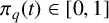 $\pi _{q}(t) \in [0,1]$
, it corresponds to a proportional reinsurance cover. In this case, the cedent should divert part of the premium to the reinsurer at the rate of
 $(1+\eta )(1-\pi _{q}(t))a$
, where
 $\eta $
is the safety loading of the reinsurer satisfying
 $\eta>\theta >0$
. Then, the cedent pays
 $100\pi _{q}(t)\%$
of the claim while the reinsurer pays
 $100(1-\pi _{q}(t))\%$
of the claim. Note that
 $\pi _{q}(t) \in (1,+\infty )$
refers to acquiring new business [Reference Bäuerle3]. After taking such a reinsurance strategy
 $\pi _{q}(t)$
into consideration, the insurer’s surplus process can be described by
 $$ \begin{align*} d R(t) &=(1+\theta) a \,d t-(1+\eta)(1-\pi_{q}(t)) a \,d t-\pi_{q}(t)\, d C(t) \nonumber \\ &=[\theta-\eta+\eta \pi_{q}(t)] a \,d t+\pi_{q}(t) \sigma_{1} \,d W_{1}(t). \end{align*} $$
Apart from reinsurance, the insurer can also invest in the financial market consisting of a risk-free bond and a risky stock. The price process of the risk-free bond
 $B(t)$
under measure
 $\mathbb {P}$
evolves according to
 $$ \begin{align*} d B(t)=r_0 B(t) \,d t, \end{align*} $$
where
 $r_0>0$
denotes the risk-free interest rate. The price process of the stock
 $S(t)$
under measure
 $\mathbb {P}$
evolves according to
 $$ \begin{align*} d S(t)=S(t) \mu \,d t+ S(t)\sigma_{2}\,d W_{2}(t), \end{align*} $$
where
 $\mu \in \mathbb {R}$
and
 $\sigma _{2}>0$
are the expected return and volatility of stock, respectively, and
 $W_{2}(t)$
is another standard Brownian motion which is independent of
 $W_{1}(t)$
.
We denote
 $\pi _s(t)$
by the amount of money the insurer invested in the stock at time t, and
 $X^{\pi }(t)$
the insurance surplus process under the reinsurance-investment strategy
 $\pi :=(\pi _q(t), \pi _s(t))$
. Apart from the investment on the stock, the insurer invests the rest of the surplus
 $X^{\pi }(t)-\pi _s(t)$
to the risk-free bond. Thus, the dynamics of wealth process
 $X^{\pi }(t)$
satisfies
 $$ \begin{align*} d X^{\pi}(t)&=[r_0 X^{\pi}(t)+(\mu-r_0) \pi_s(t)+(\theta-\eta+\eta \pi_q(t))a] \,d t \nonumber \\ &\quad +\pi_q(t) \sigma_{1}\,d W_{1}(t) + \pi_s(t) \sigma_{2}\,d W_{2}(t). \end{align*} $$
In fact, due to the bounded memory feature, the insurer’s strategies depend on the exogenous capital instantaneous inflow into or outflow from current wealth. Similar to [Reference Chunxiang and Li7], let
 $Y^{\pi }(t)$
,
 $\bar {Y}^{\pi }(t)$
and
 $Z^{\pi }(t)$
respectively reflect the integrated, average and pointwise delayed information of the wealth process in the past period
 $[t-h,t]$
with form given by
 $$ \begin{align*} Y^{\pi}(t)=\int_{-h}^{0} e^{\delta \theta} X(t+\theta)\, d \theta, \quad \bar{Y}^{\pi}(t)=\frac{Y^{\pi}(t)}{\int_{-h}^{0} e^{\delta \theta} \,d \theta}, \quad Z^{\pi}(t)=X^{\pi}(t-h), \end{align*} $$
where
 $\theta $
and
 $h>0$
are the given average parameter and delay parameter, respectively, and a capital inflow/outflow function f is a linear combination of
 $Y^{\pi }(t)$
,
 $\bar {Y}^{\pi }(t)$
and
 $Z^{\pi }(t)$
. More specifically, f satisfies
 $$ \begin{align} f(t, X^{\pi}(t)-\bar{Y}^{\pi}(t), X^{\pi}(t)-Z^{\pi}(t)) &=\alpha_{1}(X^{\pi}(t)-\bar{Y}^{\pi}(t))+\alpha_{2}(X^{\pi}(t)-Z^{\pi}(t)) \nonumber \\ &=\alpha_{1}\bigg(X^{\pi}(t)-\frac{Y^{\pi}(t)}{\int_{-h}^{0} e^{\delta \theta}\, d \theta}\bigg)+\alpha_{2}(X^{\pi}(t)-Z^{\pi}(t)) \nonumber \\ &=(\alpha_{1}+\alpha_{2}) X^{\pi}(t)-\tilde{\alpha}_{1} Y^{\pi}(t)-\alpha_{2} Z^{\pi}(t), \end{align} $$
where
 $\alpha _{1} \ge 0$
and
 $\alpha _{2} \ge 0$
, and
 $$ \begin{align*} \tilde{\alpha}_{1}=\frac{\alpha_{1}}{\int_{-h}^{0} e^{\delta \theta}\, d \theta}, \end{align*} $$
where
 $\delta>0$
is a constant average parameter and
 $h>0$
is the delay parameter. The
 $e^{\delta \theta }$
in the integral term represents the exponential decay factor. Here,
 $X^{\pi }(t)-\bar {Y}^{\pi }(t)$
reflects the average performance of wealth from
 $t-h$
to t, and
 $X^{\pi }(t)-Z^{\pi }(t)$
reflects the absolute performance of wealth in the interval
 $[t-h,t]$
.
With a little abuse of notation, the delayed wealth process of the insurer is still denoted by
 $X^{\pi }(\cdot )$
, then the delayed wealth process of the insurer is governed by
 $$ \begin{align} d X^{\pi}(t)&=[r_0 X^{\pi}(t)+(\mu-r_0) \pi_s(t)+(\theta-\eta+\eta \pi_q(t))a] \,d t + \pi_q(t)\sigma_{1}d W_{1}(t) \nonumber \\ &\quad +\pi_s(t) \sigma_{2}\,d W_{2}(t)-f(t, X^{\pi}(t)-\bar{Y}^{\pi}(t), X^{\pi}(t)-Z^{\pi}(t))\,d t. \end{align} $$
Substituting (2.1) into (2.2), we have the delayed wealth equation satisfying
 $$ \begin{align*} d X^{\pi}(t) &=[r_1 X^{\pi}(t)+\tilde{\alpha}_{1} Y^{\pi}(t)+\alpha_{2} Z^{\pi}(t)+ (\mu-r_0)\pi_s(t)+(\theta-\eta+\eta \pi_q(t))a ]\, d t \nonumber \\ & \quad + \pi_q(t) \sigma_{1}\,d W_{1}(t) + \pi_s(t) \sigma_{2}\,d W_{2}(t), \end{align*} $$
where
 $r_1=r_0-\alpha _{1}-\alpha _{2}$
. We assume that when
 $t \in [-h, 0]$
,
 $X(t)=x_0>0$
, in other words, the insurance company already has wealth
 $x_0$
at time t and has not conducted any business operations during the time period
 $[-h, 0]$
.
To introduce the ambiguity on the insurance and financial risks, we define a set of prior probability measures as below. We call the probability distortion function
 $\phi :=(\phi _{1}(t), \phi _{2}(t))_{t \in [0, T]} \in \Theta $
if
 $\phi _{1}(t)$
,
 $\phi _{2}(t)$
are deterministic functions of t and satisfy
 $$ \begin{align*} \exp \bigg\{\!\int_{t}^{T} \frac{\phi^{2}_{1}(s)+\phi^{2}_{2}(s)}{2}\, {d} s\bigg\}<\infty \end{align*} $$
for any
 $t\in [0,T]$
. Each probability distortion function
 $\phi \in \Theta $
is associated with a probability measure
 $\mathbb {Q}^{\phi } \sim \mathbb {P}$
. Additionally, the Radon–Nikodym derivative process
 $({{d} \mathbb {Q}^{\phi }}/{{d} \mathbb {P}})|_{\mathcal {F}(t)}:=\Lambda ^{\phi }(t)$
is given by
 $$ \begin{align*} \begin{aligned} \Lambda^{\phi}(t) =\exp \bigg\{\!&-\int_{0}^{t} \phi_{1}(s) \,{d} W_{1}(s)-\dfrac{1}{2} \int_{0}^{t} \phi^{2}_{1}(s) \,{d} s \\ &-\int_{0}^{t} \phi_{2}(s) \,{d} W_{2}(s)-\dfrac{1}{2} \int_{0}^{t} \phi^{2}_{2}(s) \,{d} s\bigg\}. \end{aligned} \end{align*} $$
Then, we define a set of prior probability measures by
 $\mathcal {Q}=\{\mathbb {Q}^{\phi }: \phi \in \Theta \}$
. It is obvious that
 $\mathbb {P} \in \mathcal {Q}$
is established.
Applying Girsanov’s theorem [Reference Øksendal and Sulem19], it is clear that
 $$ \begin{align} \begin{cases} d W_{1}^{\phi}(t)=d W_{1}(t)+\phi_{1}(t) \,d t,\\ d W_{2}^{\phi}(t)=d W_{2}(t)+\phi_{2}(t) \,d t, \end{cases} \end{align} $$
are
 $\mathbb {Q}^{\phi }$
-Brownian motions.
Using (2.3), it is easy to see that the dynamics of the surplus process
 $X^{\pi }(t)$
under
 $\mathbb {Q}^{\phi }$
is governed by
 $$ \begin{align} d X^{\pi}(t)&=[r_1 X^{\pi}(t)+\tilde{\alpha}_{1} Y^{\pi}(t)+\alpha_{2} Z^{\pi}(t)+ (\mu-r_0)\pi_s(t)+(\theta-\eta+\eta \pi_q(t))a \nonumber \\ &\quad -\pi_q(t) \sigma_{1} \phi_{1}(t)-\pi_{s}(t) \sigma_{2} \phi_{2}(t) ] \,d t+\pi_q(t) \sigma_{1} \,d W_{1}^{\phi}(t)+\pi_{s}(t) \sigma_{2} \,d W_{2}^{\phi}(t), \end{align} $$
in which we, by simple calculation, get that
 $Y^{\pi }(t)$
satisfies
 $$ \begin{align*} d Y^{\pi}(t)=[X^{\pi}(t)-\delta Y^{\pi}(t)-e^{-\delta h} Z^{\pi}(t)] \,d t. \end{align*} $$
Definition 2.1. A trading strategy
 $\pi =\{(\pi _{s}(t), \pi _{q}(t))\}_{t \in [0, T]}$
is said to be admissible if it satisfies the following conditions:
-
(1)
 $(\pi _{s}(t), \pi _{q}(t))$
is
$\mathbb {Q}$
-predictable;
-
(2) for all
$t \in [0, T], \pi _{q}(t) \geq 0$
; -
(3) for any
$(t, x, y) \in [0, T] \times \mathbb {R} \times \mathbb {R}$
, the following holds:
$$ \begin{align*} \mathbb{E}_{t, x,y}^{\underline{\phi}^{\pi}}\bigg[\!\int_{0}^{T}(\pi^{2}_{s}(t)+\pi^{2}_{q}(t)) \,d t\bigg]<\infty\quad \text{and} \quad \mathbb{E}_{t, x, y}^{\overline{\phi}^{\pi}}\bigg[\!\int_{0}^{T}(\pi^{2}_{s}(t)+\pi^{2}_{q}(t)) \,d t\bigg]<\infty; \end{align*} $$
-
(4)
$(\pi , X^{\pi })$
is the unique strong solution to the stochastic differential equation (2.4).
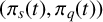





For any initial condition
 $(t, x, y) \in [0, T] \times \mathbb {R} \times \mathbb {R}$
, the corresponding set of all admissible strategies is denoted by
 $\Pi (t, x, y)$
.
Remark 2.2.
 $E^{\phi ^\pi }_{t,x,y}$
denotes the conditional expectation given that the “nature” adopts the worst-case scenario strategy
 $\phi ^\pi $
, and similarly,
 $E^{\bar {\phi }^\pi }_{t,x,y}$
corresponds to the best-case scenario strategy
 $\bar {\phi }^\pi $
. This reflects the noncooperative game nature of the alpha-max/min criterion between the investor and the “nature”.
2.2 Optimization problem under alpha-max/min mean-variance
Unlike in [Reference Bi, Meng and Zhang4, Reference Lin and Qian16, Reference Zeng and Li29, Reference Zeng, Li and Lai30], where the optimization problems were considered under the mean-variance criterion, in this paper, we study the optimization problem under the
 $\alpha $
-max/min mean-variance criterion proposed by Li et al. [Reference Li, Li and Xiong11]. Define the
 $\alpha $
-max/min mean-variance optimization problem for a controlled wealth process
 $X^{\pi }$
by
 $$ \begin{align} J_{\alpha}^{\pi}(t, x, y) &=\alpha \inf _{\phi \in \Theta} {\underline{J}}^{\pi, \phi}(t, x, y)+\hat{\alpha} \sup _{\phi \in \Theta} \overline{J}^{\pi, \phi}(t, x, y) \nonumber \\ &= \alpha {\underline{J}}^{\pi, {\underline{\phi}}^{\pi}}(t, x, y)+\hat{\alpha}\overline{J}^{\pi, \overline{\phi}^{\pi}}(t, x, y), \end{align} $$
where
 $\hat {\alpha }=1-\alpha $
and
 $\alpha \in [0,1]$
,
 $$ \begin{align} \underline{J}^{\pi, \phi}(t, x, y)&=\mathbb{E}_{t, x, y}^{\phi}[X^{\pi}(T)+\lambda Y^{\pi}(T)] \nonumber \\ &\quad -\frac{\gamma}{2} \operatorname{Var}_{t, x, y}^{\phi}[X^{\pi}(T)+\lambda Y^{\pi}(T)]+\int_{t}^{T} h_{\beta}(\phi(s)) \,{d} s \end{align} $$
and
 $$ \begin{align} \overline{J}^{\pi, \phi}(t, x, y)&=\mathbb{E}_{t, x, y}^{\phi}[X^{\pi}(T)+\lambda Y^{\pi}(T)] \nonumber \\ &\quad -\frac{\gamma}{2} \operatorname{Var}_{t, x, y}^{\phi}[X^{\pi}(T)+\lambda Y^{\pi}(T)]-\int_{t}^{T} h_{\beta}(\phi(s)) \,{d} s \end{align} $$
with
 $\mathbb {E}_{t, x, y}^{\phi }[\cdot ]$
and
 $\operatorname {Var}_{t, x, y}^{\phi }[\cdot ]$
being denoted by
 $$ \begin{align*} \mathbb{E}_{t, x, y}^{\phi}[\cdot]=\mathbb{E}^{\phi}[\cdot \mid X^{\pi}(t)=x, Y^{\pi}(t)=y],\quad \operatorname{Var}_{t, x, y}^{\phi}[\cdot]=\operatorname{Var}^{\phi}[\cdot \mid X^{\pi}(t)=x, Y^{\pi}(t)=y], \end{align*} $$
and
 $\gamma>0$
is the insurer’s risk aversion coefficient. Here, the constant
 $\lambda (\geqslant 0)$
is the weight of
 $X^{\pi }(T)$
and
 $Y^{\pi }(T)$
. By introducing the weight
 $\lambda (\geqslant 0)$
, taking into account the terminal wealth
 $X^{\pi }(T)$
and the accumulated wealth
 $Y^{\pi }(T)$
in the time period
 $[T-h,T]$
, this can help us make relevant decisions more reasonably. Additionally,
 $\underline {\phi }^{\pi }$
and
 $\overline {\phi }^{\pi }$
represent the probability distortion functions to achieve the infimum and supremum in (2.5), respectively. And the penalty function is selected as
 $$ \begin{align} h_{\beta}(\phi(s))=\frac{\phi^{2}_{1}(s)}{2 \beta_{1}}+\frac{\phi^{2}_{2}(s)}{2 \beta_{2}}. \end{align} $$
The aim of the insurer is to find the equilibrium strategy to maximize the
 $\alpha $
-max/min robust reinsurance–investment problem, that is,
 $$ \begin{align} \sup _{\pi \in \Pi} J_{\alpha}^{\pi}(t, x, y), \end{align} $$
in which the equilibrium strategy is defined as follows.
Definition 2.3. For any fixed initial state
 $(t, x, y) \in [0, T] \times \mathbb {R} \times \mathbb {R}$
, consider an admissible strategy
 $\pi ^{*}(t, x, y)$
. Choose three fixed numbers
 $\tilde {\pi }_{s} \in \mathbb {R}, \widetilde {\pi }_{q} \in \mathbb {R}_{+}$
and
 $\epsilon \in \mathbb {R}_{+}$
, and define the following strategy:
 $$ \begin{align*} \pi^{\epsilon}(s):= \begin{cases} (\widetilde{\pi}_{s}, \widetilde{\pi}_{q}) & \text { for }s \in[t, t+\epsilon), \\ \pi^{*}(s) & \text { for }s \in[t+\epsilon, T]. \end{cases} \end{align*} $$
If it holds that
 $$ \begin{align*} \lim _{\epsilon \rightarrow 0} \inf \frac{J_{\alpha}^{\pi^{*}}(t, x, y )-J_{\alpha}^{\pi^{\epsilon}}(t, x, y)}{\epsilon} \geq 0 \end{align*} $$
for all
 $(\widetilde {\pi }_{s}, \widetilde {\pi }_{q}) \in \mathbb {R} \times \mathbb {R}_{+}$
and
 $(t, x, y) \in [0, T] \times \mathbb {R} \times \mathbb {R}$
. Then,
 $\pi ^{*}(t, x, y)$
is called an equilibrium strategy and
 $J_{\alpha }^{\pi ^{*}}(t, x, y)$
is the associated equilibrium value function.
The equilibrium strategy is time-consistent, and hereafter, we call the equilibrium strategy
 $\pi ^{*}$
and the corresponding equilibrium value function
 $J_{\alpha }^{\pi ^{*}}(t, x, y)$
as the optimal time-consistent strategy and the value function for (2.9), respectively.
3 The main results
In this section, we give the verification theorem and derive the closed-form solutions. Before that, denote
 $$ \begin{align*} \begin{split} C^{1,2,1}([0, T] \times \mathbb{R} \times \mathbb{R}):=\{&\varphi(t, x, y) \mid \varphi(\cdot, x, y) \text{ is continuously differentiable on } [0, T],\\ &\varphi(t, \cdot, y) \text{ is twice continuously differentiable on } \mathbb{R}, \\ &\varphi(t, x, \cdot) \text{ is continuously differentiable on } \mathbb{R}\}, \end{split} \end{align*} $$
and for any
 $\psi (t, x, y)\in C^{1,2,1}([0, T] \times \mathbb {R} \times \mathbb {R})$
and
 $\pi \in \Pi (t, x, y)$
, define the infinitesimal generator as
 $$ \begin{align} \mathcal{A}^{\pi, \phi}\psi(t, x, y)&=\psi_{t}+[r_1 x+\tilde{\alpha}_{1} y+\alpha_{2} z+\pi_{s}(\mu-r_0)+ (\theta-\eta+\eta \pi_{q}) a-\pi_{s} \sigma_{2} \phi_{1}(t) \nonumber \\ &\quad -\pi_{s} \sigma_{2} \phi_{2}(t)]\psi_{x}+(x-\delta y-e^{-\delta h} z)\psi_{y}+(\tfrac{1}{2} \pi_{q}^{2}\sigma_{1}^{2}+\tfrac{1}{2} \pi_{s}^{2} \sigma_{2}^{2}) \psi_{x x}. \end{align} $$
3.1 Verification theorem
Now, we give the following verification theorem, which is inspired by Li et al. [Reference Li, Li and Xiong11]. For the convenience of writing, we denote
 $X^{\cdot }(\cdot )+\lambda Y^{\cdot }(\cdot )$
by
 $\Upsilon ^{\cdot }(\cdot )$
in this subsection and in Appendix A.
Theorem 3.1. For (2.9), suppose that there exist
 $V(t, x, y)$
,
 $\underline {g}(t, x, y)$
,
 $\overline {g}(t, x, y)\in C^{1,2,1}([0, T] \times \mathbb {R} \times \mathbb {R})$
satisfying the following conditions.
-
(1) For any
$(t, x, y) \in [0, T] \times \mathbb {R} \times \mathbb {R}$
, (3.2)and
$$ \begin{align} 0=\sup_{\pi \in \Pi}\bigg\{&\alpha \inf _{\phi \in \Theta}\bigg[\mathcal{A}^{\pi, \phi} V(t, x, y)-\dfrac{\gamma}{2} \mathcal{A}^{\pi, \phi} \underline{g}^{2}(t, x, y)\nonumber\\& +\gamma \underline{g}(t, x, y) \mathcal{A}^{\pi, \phi} \underline{g}(t, x, y)+h_{\beta}(\phi(t))\bigg] \nonumber \\& +\hat{\alpha} \sup _{\phi \in \Theta}\bigg[\mathcal{A}^{\pi, \phi} V(t, x, y)-\dfrac{\gamma}{2} \mathcal{A}^{\pi, \phi} \overline{g}^{2}(t, x, y)\nonumber\\& +\gamma \overline{g}(t, x, y) \mathcal{A}^{\pi, \phi} \overline{g}(t, x, y)-h_{\beta}(\phi(t))\bigg]\bigg\}, \end{align} $$
$(\pi ^{*}, \underline {\phi }^{*}, \overline {\phi }^{*})$
denote the optimal values to achieve the supremum in
$\pi $
, infimum and supremum in
$\phi $
, respectively.
-
(2) For any
$(t, x, y) \in [0, T] \times \mathbb {R} \times \mathbb {R}$
, (3.3)
$$ \begin{align} \begin{cases} V(T, x, y)=x+\lambda y, \\ \mathcal{A}^{\pi^{*}, \underline{\phi}^{*}} \underline{g}(t, x, y)=\mathcal{A}^{\pi^{*}, \overline{\phi}^{*}} \overline{g}(t, x, y)=0, \\ \underline{g}(T, x, y)=\overline{g}(T, x, y)=x+\lambda y. \end{cases} \end{align} $$
-
(3) For any
$(t, x, y) {\kern-1pt}\in{\kern-1pt} [0, T] {\kern-1pt}\times{\kern-1pt} \mathbb {R} {\kern-1pt}\times{\kern-1pt} \mathbb {R}$
,
$\pi ^{*}(t)$
,
$\overline {\phi }^{*}(t)$
,
$\underline {\phi }^{*}(t)$
,
$\mathcal {A}^{\pi ^{*}, \underline {\phi }^{*}} V(t, x, y)$
,
$\mathcal {A}^{\pi ^{*}, \overline {\phi }^{*}} V(t, x, y)$
,
$\mathcal {A}^{\pi ^{*}, \underline {\phi }^{*}} \underline {g}^{2}(t, x, y)$
and
$\mathcal {A}^{\pi ^{*}, \overline {\phi }^{*}} \overline {g}^{2}(t, x, y)$
are all deterministic functions of t and independent of x and y. -
(4)
$\underline {\phi }^{*}=\underline {\phi }^{\pi ^{*}}$
and
$\overline {\phi }^{*}=\overline {\phi }^{\pi ^{*}}$
.


Then,
 $\pi ^{*}$
is the equilibrium strategy and
 $V(t, x, y)=J_{\alpha }^{\pi ^{*}}(t, x, y)$
is the equilibrium value function to the
 $\alpha $
-robust reinsurance–investment problem (2.9). In addition,
 $\underline {g}(t, x, y)=\mathbb {E}_{t, x, y}^{\underline {\phi }^{*}}[\Upsilon ^{\pi ^{*}}(T)]$
and
 $\overline {g}(t, x, y)=\mathbb {E}_{t, x, y}^{\overline {\phi }^{*}}[\Upsilon ^{\pi ^{*}}(T)]$
.
Remark 3.2. See the references (for example, [Reference Fleming and Soner9, Reference Yong and Zhou27]) that support the existence and uniqueness of a classical solution under our model’s conditions, or note that the solution can be understood in the viscosity sense if regularity conditions are relaxed.
3.2 Closed-form solutions
In this section, we derive the optimal time-consistent reinsurance and investment strategies and the corresponding equilibrium value functions for (2.9). Suppose that
 $V(t,x,y), \underline {g}(t,x,y), \overline {g}(t,x,y), \underline {\phi }^{*}, \overline {\phi }^{*}$
satisfy conditions (1) and (2) of Theorem 3.1. Then, with some calculations, we can rewrite (3.2) as
 $$ \begin{align} 0 =\sup_{\pi \in \Pi}\bigg\{&V_{t}+[r_1 x+\tilde{\alpha}_{1}y+\alpha_{2} z+(\mu-r_0) \pi_{s}+(\theta-\eta+\eta \pi_{q}) a] V_{x} \nonumber \\ &+(x-\delta y-e^{-\delta h} z)V_{y}+\tfrac{1}{2}(\pi_{q}^{2} \sigma_{1}^{2} +\pi_{s}^{2} \sigma_{2}^{2})(V_{x x}-\alpha \gamma \underline{g}_{x}^{2}-\hat{\alpha} \gamma \overline{g}_{x}^{2}) \nonumber \\ &+\alpha \inf_{\phi \in \Theta}\{-(\pi_{q} \sigma_{1} \phi_{1}+\pi_{s} \sigma_{2} \phi_{2}) V_{x}+h_{\beta}(\phi)\} \nonumber \\ &+\hat{\alpha} \sup_{\phi \in \Theta}\{-(\pi_{q} \sigma_{1} \phi_{1}+\pi_{s} \sigma_{2} \phi_{2}) V_{x}-h_{\beta}(\phi)\}\bigg\}. \end{align} $$
Applying the first-order condition in (3.4) with respect to
 $\phi $
gives
 $$ \begin{align} \begin{cases} \underline{\phi}_{1}^{*}=\beta_{1}\pi_{q} \sigma_{1} V_{x}, \\ \underline{\phi}_{2}^{*}=\beta_{2} \pi_{s} \sigma_{2} V_{x}, \end{cases} \end{align} $$
and
 $$ \begin{align} \begin{cases} \overline{\phi}_{1}^{*}=-\beta_{1}\pi_{q} \sigma_{1} V_{x}, \\ \overline{\phi}_{2}^{*}=-\beta_{2} \pi_{s} \sigma_{2} V_{x}. \end{cases} \end{align} $$
Substituting (3.5) and (3.6) into (3.4) yields
 $$ \begin{align} 0 =\sup_{\pi \in \Pi}\bigg\{&V_{t}+[r_1 x+\tilde{\alpha}_{1}y+\alpha_{2} z+(\mu-r_0) \pi_{s}+(\theta-\eta+\eta \pi_{q}) a] V_{x} \nonumber \\ &+(x-\delta y-e^{-\delta h} z)V_{y}+\dfrac{1}{2}(\pi_{q}^{2} \sigma_{1}^{2} +\pi_{s}^{2} \sigma_{2}^{2})(V_{x x}-\alpha \gamma \underline{g}_{x}^{2}-\hat{\alpha} \gamma \overline{g}_{x}^{2}) \nonumber \\ &+\dfrac{1-2 \alpha}{2}(\beta_{1} \pi_{q}^{2} \sigma_{1}^{2}+\beta_{2} \pi_{s}^{2} \sigma_{2}^{2} ) V_{x}^{2}\bigg\}. \end{align} $$
By the first-order condition and differentiating with respect to
 $\pi _{q}(t)$
and
 $\pi _{s}(t)$
in (3.7), respectively we obtain
 $\pi _{q}^{*}(t)$
and
 $\pi _{s}^{*}(t)$
as follows:
 $$ \begin{align} \pi_{q}^{*}=\frac{\eta a V_{x}}{\sigma_{1}^{2}[\alpha \gamma \underline{g}_{x}^{2}+\hat{\alpha} \gamma \overline{g}_{x}^{2}-V_{x x}+(2 \alpha-1) \beta_{1} V_{x}^{2}]} \end{align} $$
and
 $$ \begin{align} \pi_{s}^{*}=\frac{(\mu-r_0) V_{x}}{\sigma_{2}^{2}[\alpha \gamma \underline{g}_{x}^{2}+\hat{\alpha} \gamma \overline{g}_{x}^{2}-V_{x x}+(2 \alpha-1) \beta_{2} V_{x}^{2}]}. \end{align} $$
Inspired by the boundary conditions (3.3), we assume the solutions of (3.7) of the forms
 $$ \begin{align} \begin{cases} V(t, x, y) =A(t)(x+\lambda y)+B(t), \\ \underline{g}(t, x, y)=\underline{a}(t) (x+\lambda y)+\underline{b}(t), \\ \overline{g}(t, x, y)=\overline{a}(t) (x+\lambda y)+\overline{b}(t), \end{cases} \end{align} $$
where
 $A(t), B(t), \underline {a}(t), \underline {b}(t), \overline {a}(t), \overline {b}(t)$
are functions of t. By the first and the third relation of (3.3), the boundary conditions are given by
 $$ \begin{align*} A(T)=\underline{a}(T)=\overline{a}(T)=1 \quad \text{and} \quad B(T)=\underline{b}(T)=\overline{b}(T)=0. \end{align*} $$
Substituting (3.10) into (3.7) yields
 $$ \begin{align} 0&=A^{\prime} (x+\lambda y)+B^{\prime}+[(r_1+\lambda) x+(\tilde{\alpha}_{1}-\lambda \delta) y+(\alpha_{2}-\lambda e^{-\delta h}) z]\, A \nonumber \\ &\quad +[(\mu-r_0) \pi_{s}^{*}+(\theta-\eta+\eta \pi_{q}^{*}) a]\,A-\dfrac{1}{2} ({\pi_{q}^{*}}^{2} \sigma_{1}^{2}+{\pi_{s}^{*}}^{2} \sigma_{2}^{2}) (\alpha \gamma \underline{a}^{2}+\hat{\alpha}\gamma \overline{a}^{2}) \nonumber \\ &\quad +\frac{1-2 \alpha}{2}[\beta_{1} {\pi_{q}^{*}}^{2} \sigma_{1}^{2}+\beta_{2} {\pi_{s}^{*}}^{2} \sigma_{2}^{2} ]\,A^{2}. \end{align} $$
By virtue of Pang and Hussain [Reference Pang and Hussain20], we assume the value function is independent of z. Suppose
 $$ \begin{align*} \alpha_{2}=\lambda e^{-\delta h} \end{align*} $$
and
 $$ \begin{align*} \tilde{\alpha}_{1}-\delta e^{\delta h}\alpha_{2}=(r_1+e^{\delta h}\alpha_{2})e^{\delta h}\alpha_{2}. \end{align*} $$
Remark 3.3. These assumptions are strong. Their primary purpose is to ensure the mathematical tractability of the extended HJB equation (see [Reference Pang and Hussain20]), specifically to guarantee the existence of a unique and well-defined solution to the system of equations (3.12). More importantly, we give a subsection in the numerical analysis section (Section 4) to discuss the economic interpretation and practical plausibility of these parameters. We demonstrate through numerical ranges that these assumptions can be satisfied under realistic market conditions, and we analyse how the equilibrium strategy behaves when the parameters approach the boundaries of these assumptions.
Let
 $x+\lambda y=u$
, then we can rewrite (3.11) as
 $$ \begin{align} 0&=A^{\prime} u+B^{\prime}+[(r_1+\lambda) u+(\mu-r_0) \pi_{s}^{*}+(\theta-\eta+\eta \pi_{q}^{*}) a]\,A \nonumber \\ &\quad -\dfrac{1}{2} ({\pi_{q}^{*}}^{2} \sigma_{1}^{2}+{\pi_{s}^{*}}^{2} \sigma_{2}^{2}) (\alpha \gamma \underline{a}^{2}+\hat{\alpha}\gamma \overline{a}^{2})+\frac{1-2 \alpha}{2}[\beta_{1} {\pi_{q}^{*}}^{2} \sigma_{1}^{2}+\beta_{2} {\pi_{s}^{*}}^{2} \sigma_{2}^{2} ]\,A^{2}. \end{align} $$
Substituting (3.8) and (3.9) into (3.12) yields
 $$ \begin{align} 0&=A^{\prime} u+B^{\prime}+[(r_1+\lambda) u+(\theta-\eta) a]\,A+\frac{\eta^{2} a^{2} A^{2}}{2\sigma_{1}^{2}[\alpha \gamma \underline{a}^{2}+\hat{\alpha} \gamma \overline{a}^{2}+(2 \alpha-1) \beta_{1} A^{2}]} \nonumber \\ &\quad +\frac{(\mu-r_0)^{2} A^{2}}{2\sigma_{2}^{2}[\alpha \gamma \underline{a}^{2}+\hat{\alpha} \gamma \overline{a}^{2}+(2 \alpha-1) \beta_{2} A^{2}]}. \end{align} $$
Similarly, substituting (3.8), (3.9) and (3.10) into the second relation of (3.3) yields
 $$ \begin{align} 0&=\underline{a}^{\prime} u+\underline{b}^{\prime}+[(r_1+\lambda) u +(\mu-r_0) \pi_{s}^{*} \nonumber \\&\quad+(\theta-\eta+\eta \pi_{q}^{*}) a- {\pi_{q}^{*}}^{2} \sigma_{1}^{2}\beta_{1}A- {\pi_{s}^{*}}^{2} \sigma_{2}^{2}\beta_{2}A]\underline{a},\end{align} $$
 $$\begin{align} 0&=\overline{a}^{\prime} u+\overline{b}^{\prime}+[(r_1+\lambda) u+(\mu-r_0) \pi_{s}^{*} \nonumber \\&\quad+(\theta-\eta+\eta \pi_{q}^{*}) a+ {\pi_{q}^{*}}^{2} \sigma_{1}^{2}\beta_{1}A+ {\pi_{s}^{*}}^{2} \sigma_{2}^{2}\beta_{2}A]\overline{a}. \end{align} $$
By matching the coefficients of the terms of u,
 $$ \begin{align*} A(t)^{\prime}+(r_1+\lambda) A(t)=\underline{a}(t)^{\prime}+(r_1+\lambda) \underline{a}(t)=\overline{a}(t)^{\prime}+(r_1+\lambda) \overline{a}(t)=0. \end{align*} $$
We use boundary conditions
 $A(T)=\underline {a}(T)=\overline {a}(T)=1$
to get
 $$ \begin{align} A(t)=\underline{a}(t)=\overline{a}(t)= e^{(r_1+\lambda)(T-t)}, \quad t \in[0, T]. \end{align} $$
Substituting (3.16) back into (3.13)–(3.15), and using the boundary condition
 $B(T)=\underline {b}(T)=\overline {b}(T)=0$
, we can easily obtain the explicit solution of
 $B(t), \underline {b}(t)$
and
 $\overline {b}(t)$
:
 $$ \begin{align} B(t)=\frac{a(\theta-\eta)}{(r_1+\lambda)}(e^{(r_1+\lambda)(T-t)}-1)+\frac{\eta^{2} a^{2} (T-t)}{2\sigma_{1}^{2}[\gamma+(2 \alpha-1) \beta_{1}]}+\frac{(\mu-r_0)^{2} (T-t)}{2\sigma_{2}^{2}[ \gamma+(2 \alpha-1) \beta_{2} ]}, \end{align} $$
and the expressions of
 $\underline {b}(t)$
and
 $\overline {b}(t)$
are given by
 $$ \begin{align*} \underline{b}(t)&=\frac{a(\theta-\eta)}{(r_1+\lambda)}(e^{(r_1+\lambda)(T-t)}-1)+\frac{\eta^{2} a^{2} [\gamma+(2 \alpha-2) \beta_{1}](T-t)}{\sigma_{1}^{2}[\gamma+(2 \alpha-1) \beta_{1}]^2} \nonumber \\ &\quad +\frac{(\mu-r_0)^{2}[ \gamma+(2 \alpha-2) \beta_{2}] (T-t)}{\sigma_{2}^{2}[ \gamma+(2 \alpha-1) \beta_{2}]^2},\\ \overline{b}(t) &=\frac{a(\theta-\eta)}{(r_1+\lambda)}(e^{(r_1+\lambda)(T-t)}-1)+\frac{\eta^{2} a^{2} (\gamma+2 \alpha \beta_{1})(T-t)}{\sigma_{1}^{2}[\gamma+(2 \alpha-1) \beta_{1}]^2} \nonumber \\ &\quad +\frac{(\mu-r_0)^{2}(\gamma+2 \alpha \beta_{2}) (T-t)}{\sigma_{2}^{2}[\gamma+(2 \alpha-1) \beta_{2}]^2}. \end{align*} $$
Thus, the explicit expression of the value function is obtained. We state the equilibrium strategy for the optimal control problem (2.9) in the following theorem.
Theorem 3.4. For the
 $\alpha $
-robust reinsurance–investment problem (2.9), the optimal reinsurance and investment strategies for the insurer are as follows.
-
(1) The equilibrium reinsurance strategy
$\pi _{q}^{*}(t)$
is given by and the equilibrium investment strategy
$$ \begin{align*} \pi_{q}^{*}(t)=\frac{\eta a}{\sigma_{1}^{2} [\gamma+(2 \alpha-1) \beta_{1}]e^{(r_1+\lambda)(T-t)}}, \end{align*} $$
$\pi _{s}^{*}(t)$
is given by
$$ \begin{align*} \pi_{s}^{*}(t)=\frac{\mu-r_0}{\sigma_{2}^{2} [\gamma+(2 \alpha-1) \beta_{2}]e^{(r_1+\lambda)(T-t)}}. \end{align*} $$
-
(2) The corresponding equilibrium value function is given by
where
$$ \begin{align*} J_{\alpha}^{\pi^{*}}(t, x, y)=e^{(r_1+\lambda)(T-t)} (x+\lambda y)+B(t), \end{align*} $$
$B(t)$
is given by (3.17).
-
(3) The associated probability distortion functions of the extremely ambiguity-averse measure and the extremely ambiguity-seeking measure are given respectively by
and
$$ \begin{align*} \begin{cases}\underline{\phi}_{1}^{*}(t)=\dfrac{\eta a \beta_1}{\sigma_{1} [\gamma+(2 \alpha-1) \beta_{1} ]}, \\ \underline{\phi}_{2}^{*}(t)=\dfrac{(\mu-r_0)\beta_{2}}{\sigma_{2} [\gamma+(2 \alpha-1) \beta_{2} ]},\end{cases} \end{align*} $$
$$ \begin{align*} \begin{cases}\overline{\phi}_{1}^{*}(t)=-\dfrac{\eta a \beta_1}{\sigma_{1} [\gamma+(2 \alpha-1) \beta_{1} ]}, \\ \overline{\phi}_{2}^{*}(t)=-\dfrac{(\mu-r_0)\beta_{2}}{\sigma_{2} [\gamma+(2 \alpha-1) \beta_{2}]}.\end{cases} \end{align*} $$


To end this section, we consider the cases of our model without ambiguity aversion or delay. Additionally, the closed-form solutions are as below.
Corollary 3.5. If the model for uncertainty is ignored (it means
 $\phi _{1}(t)=\phi _{2}(t)=0$
), then the equilibrium strategy
 $\pi _{q}^{*}(t)$
and
 $\pi _{s}^{*}(t)$
are given by
 $$ \begin{align*} \pi_{q}^{*}(t)=\frac{\eta a}{\sigma_{1}^{2} \gamma e^{(r_1+\lambda)(T-t)} }, \quad \pi_{s}^{*}(t)=\frac{\mu-r_0}{\sigma_{2}^{2} \gamma e^{(r_1+\lambda)(T-t)} }, \end{align*} $$
and the value function is given by
 $$ \begin{align*} \begin{aligned} J^{\pi^{*}}(t, x, y)&=e^{(r_1+\lambda)(T-t)} (x+\lambda y)\\ &\quad +\frac{a(\theta-\eta)}{(r_1+\lambda)}(e^{(r_1+\lambda)(T-t)}-1)+\frac{\eta^{2} a^{2} (T-t)}{2\sigma_{1}^{2} \gamma}+\frac{(\mu-r_0)^{2} (T-t)}{2\sigma_{2}^{2} \gamma}.\end{aligned} \end{align*} $$
Corollary 3.6. If the delay is ignored, then the equilibrium strategy
 $\pi _{q}^{*}(t)$
and
 $\pi _{s}^{*}(t)$
are given by
 $$ \begin{align*} \pi_{q}^{*}(t)=\frac{\eta a}{\sigma_{1}^{2} [\gamma+(2 \alpha-1) \beta_{1}] e^{r_0(T-t)} }, \quad \pi_{s}^{*}(t)=\frac{\mu-r_0}{\sigma_{2}^{2} [\gamma+(2 \alpha-1) \beta_{2}] e^{r_0(T-t)} }, \end{align*} $$
and the value function is given by
 $$ \begin{align*} \begin{aligned} J_{\alpha}^{\pi^{*}}(t, x)&=e^{r_0(T-t)} x+\frac{a(\theta-\eta)}{r_0}(e^{r_0(T-t)}-1)\\ &\quad +\frac{\eta^{2} a^{2} (T-t)}{2\sigma_{1}^{2}[\gamma+(2 \alpha-1) \beta_{1}]}+\frac{(\mu-r_0)^{2} (T-t)}{2\sigma_{2}^{2}[\gamma+(2 \alpha-1) \beta_{2}]}. \end{aligned} \end{align*} $$
4 Numerical analysis
In this section, we illustrate how the model’s parameters influence investment and reinsurance strategies. In these examples, unless otherwise stated, the basic parameters are kept as follows:
 $\alpha =0.8$
,
 $\gamma =0.5$
,
 $\eta =0.2$
,
 $\beta _1=1$
,
 $\beta _2=3$
,
 $\mu =0.1$
,
 $r_0=0.08$
,
 $\lambda =0.05$
,
 $\sigma _1=0.5$
,
 $\sigma _2=0.2$
,
 $a=1$
,
 $\delta =0.5$
,
 $h=1$
,
 $t=0$
and
 $T=10$
.
Remark 4.1. We clarify that the baseline values for financial market parameters (for example, risk-free rate
 $r_0=0.08$
, stock drift
 $\mu =0.1$
,
 $\sigma _2=0.2$
) are chosen to reflect typical market conditions, and are consistent with values used in seminal works on portfolio optimization and insurance risk management [Reference Bi, Meng and Zhang4, Reference Zeng and Li29]. Parameters specific to the insurance surplus process (for example, claim intensity a, safety loadings
 $\theta =0.2$
and
 $\eta =0.2$
,
 $\sigma _1=0.5$
) are justified by referencing standard diffusion-approximation models for insurance claims [Reference Schmidli21] and ensuring that the condition
 $\eta> \theta > 0$
(reinsurer’s loading exceeding insurer’s loading) holds for economic viability.
Note that
 $$ \begin{align*} \alpha_{2}=e^{-\delta h}\lambda, \quad \alpha_{1}=(r_0-\alpha_{2}+\lambda+\delta) \frac{\lambda \int_{-h}^{0} e^{\delta \theta} \,d \theta}{1+\lambda \int_{-h}^{0} e^{\delta \theta} \,d \theta}\quad \text{and}\quad r_1=r_0-\alpha_1-\alpha_2. \end{align*} $$
Consequently, the optimal reinsurance strategy
 $\pi _{q}^{*}(t)$
and the optimal investment strategy
 $\pi _{s}^{*}(t)$
can be rewritten as follows:
 $$ \begin{align} \pi_{q}^{*}(t)&=\frac{\eta a}{\sigma_{1}^{2} [\gamma+(2 \alpha-1) \beta_{1} ]e^{(r_{1}+\lambda)(T-t) }}, \end{align} $$
 $$ \begin{align} \pi_{s}^{*}(t)&=\frac{\mu-r_0}{\sigma_{2}^{2} [\gamma+(2 \alpha-1) \beta_{2}]e^{(r_{1}+\lambda)(T-t) }}. \end{align} $$
4.1 Analysis of the optimal reinsurance strategy
$\pi _{q}^{*}(t)$

From (4.1),
 $$ \begin{align*} &\frac{\partial \pi_{q}^{*}(t)}{\partial \beta_{1}}<0,\, \frac{\partial \pi_{q}^{*}(t)}{\partial \gamma}<0,\, \frac{\partial \pi_{q}^{*}(t)}{\partial \alpha}<0, \, \frac{\partial \pi_{q}^{*}(t)}{\partial r_{0}}<0, \\&\frac{\partial \pi_{q}^{*}(t)}{\partial \sigma_{1}}<0,\, \frac{\partial \pi_{q}^{*}(t)}{\partial t}>0,\, \frac{\partial \pi_{q}^{*}(t)}{\partial \eta}>0,\, \frac{\partial \pi_{q}^{*}(t)}{\partial a}>0, \end{align*} $$
which imply that the optimal reinsurance strategy
 $\pi _{q}^{*}(t)$
is decreasing with respect to the insurance liability ambiguity
 $\beta _{1}$
, the coefficient of risk aversion of the insurer
 $\gamma $
, the ambiguity attitude
 $\alpha $
, the risk-free interest rate
 $r_{0}$
and the volatility of the surplus process of the insurer
 $\sigma _{1}$
, but increasing with respect to the premium return rate of the reinsurer
 $\eta $
, time t and insurance claim amount a.
In Figure 1, it shows that as the parameters
 $\beta _{1}$
decreases or
 $\eta $
increases, the insurer will purchase less reinsurance or invest more on new business. As
 $\beta _1$
increases, the insurance liability is more ambiguous, then to manage the risk exposure, the insurer will also purchase more reinsurance. With the increase of
 $\eta $
, to reduce the cost compensation of reinsurance, insurers are more willing to undertake insurance business and increase the retention rate of reinsurance. In addition, as time t goes by, insurers will retain more insurance business by buying less reinsurance.
Effects of parameters
 $\beta _{1}$
, t and
 $\eta $
on
 $\pi _q^*$
.

Figure 2 shows that the optimal reinsurance strategy
 $\pi _q^*(t)$
decreases with ambiguity attitude
 $\alpha $
and risk coefficient
 $\gamma $
, while increasing with respect to the transformed weight
 $\lambda $
and insurance claim amount a. As
 $\lambda $
increases, the average delayed wealth
 $\overline {Y}(T)$
takes up a larger weight in the final performance measure. Therefore, the average effect will definitely reduce the overall risk of terminal wealth for the insurance company. That is, to achieve the same expected terminal wealth level, when
 $\lambda $
is larger, the risk can be controlled at a lower level. As
 $\alpha $
and
 $\gamma $
increase, the insurer is more ambiguity averse and risk averse, the insurer will be more conservative to undertake risk and thus purchase more reinsurance.
Effects of parameters
 $\lambda $
,
 $\gamma $
,
 $\alpha $
and a on
 $\pi _q^*$
.

Figure 3 shows that the optimal reinsurance strategy
 $\pi _q^*(t)$
decreases with average parameter
 $\delta $
, the risk-free interest rate
 $r_{0}$
and the volatility of the surplus process
 $\sigma _{1}$
, while increasing with the delay parameter h. From the definition of the average delayed wealth
 $\bar {Y}(t)$
, we can see that the larger
 $\delta $
is, the smaller the weight of early wealth. In other words, wealth closer to the current time is more important in constructing the average delayed wealth
 $\bar {Y}(t)$
. As h increases, the average time range becomes longer, so the average delayed wealth is more stable.
Effects of parameters
 $\delta $
, h,
 $r_{0}$
and
 $\sigma _{1}$
on
 $\pi _q^*$
.

4.2 Analysis of the optimal investment strategy
$\pi _{s}^{*}(t)$

In this subsection, we provide some sensitivity analyses on the effect of the parameters on the optimal investment strategies
 $\pi _s^*(t)$
. From (4.2), we can derive that
 $({\partial \pi _{s}^{*}(t)}/{\partial \alpha })<0$
,
 $({\partial \pi _{s}^{*}(t)}/{\partial \beta _{2}})<0$
,
 $({\partial \pi _{s}^{*}(t)}/{\partial \sigma _{2}})<0$
,
 $({\partial \pi _{s}^{*}(t)}/{\partial \gamma })<0$
,
 $({\partial \pi _{s}^{*}(t)}/{\partial \mu })>0$
,
 $({\partial \pi _{s}^{*}(t)}/{\partial t})>0$
, which imply that the optimal investment strategy
 $\pi _{s}^{*}(t)$
decreases with respect to the ambiguity attitude
 $\alpha $
, the stock return ambiguity
 $\beta _{2}$
, the volatility of the stock volatility
 $\sigma _{2}$
and the coefficient of risk aversion of the insurer
 $\gamma $
, but increases with respect to the stock returns
 $\mu $
and time t.
Figure 4 implies that the optimal investment strategy
 $\pi _{s}^{*}(t)$
increases with
 $\mu $
, while decreases with
 $\alpha $
,
 $r_0$
and
 $\sigma _2$
. This shows that the higher the expected return on stocks, the smaller the volatility, the greater the amount invested in stocks. When
 $r_0$
and
 $\alpha $
increase, the amount invested in stocks decreases.
Effects of parameters
 $\mu $
,
 $\alpha $
,
 $\sigma _2$
and
 $r_{0}$
on
 $\pi _s^*$
.

When the average parameter
 $\delta $
decreases or the delay parameter h increases, the insurer will invest more money in the risky asset, as shown in Figure 5(a). The insurer will invest more money in the risky asset as the transformed weight
 $\lambda $
increases. This is shown in Figure 5(b).
Effects of parameters h,
 $\delta $
and
 $\lambda $
on
 $\pi _s^*$
.

Figure 6 implies that the optimal investment strategy
 $\pi _{s}^{*}(t)$
increases with t and
 $\lambda $
, and decreases with
 $\beta _2$
and
 $\gamma $
. The insurer will invest less money in the stock if they becomes more risk averse or the stock return is more ambiguous.
Effects of parameters
 $\beta _2$
, t,
 $\lambda $
and
 $\gamma $
on
 $\pi _s^*$
.

5 Conclusion
This paper studies the robust optimal reinsurance–investment problem for insurers with delay. We assume that the financial market consists of a risk-free asset and a risky asset. The explicit solution of the optimal reinsurance and investment strategy and value function is derived, and the proof of the verification theorem is given. The influence of parameters on the optimal strategy is analysed through numerical examples. There are some related issues that deserve further study. On the one hand, more complex stock models can be considered, although explicit solutions may not be possible. On the other hand, we can extend the risk aversion coefficient in the objective function of this paper from constant to more general cases, such as dependence on market state or current surplus. In addition, we only consider the optimal time-consistent strategy for the
 $\alpha $
-mean-variance problem, which can be extended to consider the optimal reinsurance and investment problems with other objectives in future studies.
Acknowledgment
This work is supported by Chongqing Social Science Planning Project under Grant 2023NDYB89.
A Proof of Theorem 3.1
The proof of Theorem 3.1 is divided into two parts. That is to say, we just need to prove the following Proposition A.2 and Proposition A.4. We first complete the proof of Proposition A.2. To do this, we need to introduce the following lemma.
Lemma A.1. Consider a deterministic strategy
 $\pi =\{\pi _{q}(t), \pi _{s}(t)\}_{t \in [0, T]}$
.
-
(1) The discounted process
$\{e^{-(r_{1}+\lambda )t}\Upsilon ^{\pi }(t)\}_{t \in [0, T]}$
has independent increments under any
$\mathbb {Q}^{\phi } \in \mathcal {Q}$
. -
(2) The function
$\overline {J}^{\pi , \overline {\phi }^{\pi }}(t, x, y)-\underline {J}^{\pi , \underline {\phi }^{\pi }}(t, x, y)$
is independent of x and y. -
(3) For any
$0 \leq t \leq w \leq T$
, the probability distortion functions corresponding to reaching the supremum and infimum in (2.5) are the same as the probability distortion functions attaining the infimum in and supremum in
$$ \begin{align*} \inf _{\phi \in \Theta}\bigg\{&\mathbb{E}^{\phi}[e^{(r_{1}+\lambda)(T-w)}\Upsilon^{\pi}(w)-e^{(r_{1}+\lambda)(T-t)}\Upsilon^{\pi}(t)]\\ &-\frac{\gamma}{2} \operatorname{Var}^{\phi}[e^{(r_{1}+\lambda)(T-w)} \Upsilon^{\pi}(w)-e^{(r_{1}+\lambda)(T-t)} \Upsilon^{\pi}(t)]+\int_{t}^{w} h_{\beta}(\phi(s)) \,{d}s\bigg\}, \end{align*} $$
which are given respectively by
$$ \begin{align*} \sup _{\phi \in \Theta}\bigg\{&\mathbb{E}^{\phi}[e^{(r_{1}+\lambda)(T-w)} \Upsilon^{\pi}(w)-e^{(r_{1}+\lambda)(T-t)} \Upsilon^{\pi}(t)]\\ &-\frac{\gamma}{2} \operatorname{Var}^{\phi}[e^{(r_{1}+\lambda)(T-w)} \Upsilon^{\pi}(w)-e^{(r_{1}+\lambda)(T-t)} \Upsilon^{\pi}(t)]-\int_{t}^{w} h_{\beta}(\phi(s)) \,{d} s\bigg\}, \end{align*} $$
(A.1)and
$$ \begin{align} \begin{cases}\underline{\phi}_{1}^{\pi}(t)=\beta_{1}\pi_{q}(t) \sigma_{1}e^{(r_{1}+\lambda)(T-t)}, \\ \underline{\phi}_{2}^{\pi}(t)=\beta_{2} \pi_{s}(t) \sigma_{2} e^{(r_{1}+\lambda)(T-t)},\end{cases} \end{align} $$
(A.2)
$$ \begin{align} \begin{cases} \overline{\phi}_{1}^{\pi}(t)=-\beta_{1}\pi_{q}(t) \sigma_{1} e^{(r_{1}+\lambda)(T-t)}, \\ \overline{\phi}_{2}^{\pi}(t)=-\beta_{2} \pi_{s}(t) \sigma_{2} e^{(r_{1}+\lambda)(T-t)}. \end{cases} \end{align} $$


Proof. (1) By applying Itô’s formula to (2.4),
 $$ \begin{align} &e^{-(r_{1}+\lambda)T} \Upsilon^{\pi}(t)-e^{-(r_{1}+\lambda)t} \Upsilon^{\pi}(t) \nonumber \\ &\quad=\int_{t}^{T} e^{-(r_{1}+\lambda)s} [(\mu-r_0)\pi_s(s)+(\theta-\eta+\eta \pi_q(s))a] \,d s \nonumber \\ &\qquad +\int_{t}^{T} e^{-(r_{1}+\lambda)s} [-\pi_q(s) \sigma_{1} \phi_{1}(s)-\pi_{s}(s) \sigma_{2} \phi_{2}(s)]\, d s \nonumber \\ &\qquad +\int_{t}^{T} e^{-(r_{1}+\lambda)s} \pi_q(s) \sigma_{1} \,d W_{1}^{\phi}(s)+\int_{t}^{T} e^{-(r_{1}+\lambda)s} \pi_s(s) \sigma_{2} \,d W_{2}^{\phi}(s). \end{align} $$
Because
 $\pi $
and
 $\phi $
are determined, it is easy to get the independent incremental property.
(2) By subtracting (2.7) from (2.6), and using
 $\overline {\phi }^{\pi }, \underline {\phi }^{\pi } \in \Theta $
,
 $$ \begin{align*} &\overline{J}^{\pi, \overline{\phi}^{\pi}}(t, x, y)-\underline{J}^{\pi, \underline{\phi}^{\pi}}(t, x, y) \nonumber \\ &\quad=\mathbb{E}_{t, x, y}^{\overline{\phi}^{\pi}}[\Upsilon^{\pi}(t)]-\mathbb{E}_{t, x, y}^{\underline{\phi}^{\pi}}[\Upsilon^{\pi}(t)]-\frac{\gamma}{2} \operatorname{Var}_{t, x, y}^{\overline{\phi}^{\pi}}[\Upsilon^{\pi}(t)] \nonumber \\ &\qquad +\frac{\gamma}{2} \operatorname{Var}_{t, x, y}^{\underline{\phi}^{\pi}}[\Upsilon^{\pi}(t)]-\int_{t}^{T} h_{\beta}(\overline{\phi}^{\pi}(s)) \,d s-\int_{t}^{T} h_{\beta}(\underline{\phi}^{\pi}(s)) \,ds. \end{align*} $$
Through part (1), we know that
 $\Upsilon ^{\pi }(t)-e^{(r_1+\lambda )(T-t)} \Upsilon ^{\pi }(t)$
and
 $\Upsilon ^{\pi }(t)$
are independent, so
 $$ \begin{align*} &\overline{J}^{\pi, \overline{\phi}^{\pi}}(t, x, y)-\underline{J}^{\pi, \underline{\phi}^{\pi}}(t, x, y)=\mathbb{E}^{\overline{\phi}^{\pi}}[\Upsilon^{\pi}(t)-e^{(r_1+\lambda)(T-t)} \Upsilon^{\pi}(t)] \nonumber \\ &\quad-\mathbb{E}^{\underline{\phi}^{\pi}}[\Upsilon^{\pi}(t)-e^{(r_1+\lambda)(T-t)} \Upsilon^{\pi}(t)]-\frac{\gamma}{2} \operatorname{Var}^{\overline{\phi}^{\pi}}[\Upsilon^{\pi}(t)-e^{(r_1+\lambda)(T-t)} \Upsilon^{\pi}(t)] \nonumber \\ &\quad+\frac{\gamma}{2} \operatorname{Var}^{\underline{\phi}^{\pi}}[\Upsilon^{\pi}(t)-e^{(r_1+\lambda)(T-t)} \Upsilon^{\pi}(t)]-\int_{t}^{T} h_{\beta}(\overline{\phi}^{\pi}(s)) \,d s-\int_{t}^{T} h_{\beta}(\underline{\phi}^{\pi}(s)) \,d s, \end{align*} $$
which is independent of x and y. Since
 $\overline {J}^{\pi , \overline {\phi }^{\pi }}(t, x, y)-\underline {J}^{\pi , \underline {\phi }^{\pi }}(t, x, y)$
is independent of x and y, we write it as
 $\overline {J}^{\pi , \overline {\phi }^{\pi }}(t, \cdot , \cdot )-\underline {J}^{\pi , \underline {\phi }^{\pi }}(t, \cdot , \cdot )$
. In the following, we use the same notation for functions that are independent of x and y.
(3) It follows from (A.3) and (2.8) that
 $$ \begin{align} \mathbb{E}^{\phi}&[e^{(r_{1}+\lambda)(T-w)} \Upsilon^{\pi}(w)-e^{(r_{1}+\lambda)(T-t)} \Upsilon^{\pi}(t)] \nonumber \\&\quad-\frac{\gamma}{2} \operatorname{Var}^{\phi}[e^{(r_{1}+\lambda)(T-w)} \Upsilon^{\pi}(w)-e^{(r_{1}+\lambda)(T-t)} \Upsilon^{\pi}(t)] \pm \int_{t}^{w} h_{\beta}(\phi(s)) \,{d} s \nonumber \\&=\int_{t}^{w}\!\! e^{(r_{1}+\lambda)(T-s)} [(\mu-r_0)\pi_s(s)+(\theta-\eta+\eta \pi_q(s))a-\pi_q(s) \sigma_{1} \phi_{1}(s)-\pi_{s}(s) \sigma_{2} \phi_{2}(s)] \,d s \nonumber \\&\quad-\frac{\gamma}{2}\int_{t}^{w} e^{2(r_{1}+\lambda)(T-s)} [\pi^2_q(s) \sigma_{1}^2 +\pi^2_{s}(s) \sigma_{2}^2 ] \,d s \pm \int_{t}^{w} \frac{\phi^{2}_{1}(s)}{2 \beta_{1}}+\frac{\phi^{2}_{2}(s)}{2 \beta_{2}} \,d s. \end{align} $$
The variance formula of X can be found in [Reference Øksendal and Sulem19, Remark 1.18]. Applying the first-order condition to (A.4) yields the expressions for
 $\underline {\phi }^{\pi }$
and
 $\overline {\phi }^{\pi }$
given in (A.1) and (A.2), respectively. Additionally, both expressions of
 $\underline {\phi }^{\pi }$
and
 $\overline {\phi }^{\pi }$
are independent of w. By letting
 $w=T$
in (A.4),
 $$ \begin{align*} &\mathbb{E}^{\phi}[ \Upsilon^{\pi}(t)-e^{(r_{1}+\lambda)(T-t)} \Upsilon^{\pi}(t)] -\frac{\gamma}{2} \operatorname{Var}^{\phi}[\Upsilon^{\pi}(t)-e^{(r_{1}+\lambda)(T-t)} \Upsilon^{\pi}(t)] \pm \int_{t}^{T} h_{\beta}(\phi(s)) \,{d} s \nonumber \\ &\quad=E_{t, x, y}^{\phi}[\Upsilon^{\pi}(t)]-e^{(r_{1}+\lambda)(T-t)}(X+\lambda y)-\frac{\gamma}{2} \operatorname{Var}_{t, x, y}^{\phi}[\Upsilon^{\pi}(t)]\pm \int_{t}^{T} h_{\beta}(\phi(s)) \,{d} s. \end{align*} $$
We get the conclusion that
 $\underline {\phi }^{\pi }$
and
 $\overline {\phi }^{\pi }$
given in (A.1) and (A.2) also reach the infimum and supremum in (2.5), respectively. This completes the proof of the lemma.
The following proposition proves the first part of Theorem 3.1, which is the representation of the value functions
 $\underline {g}$
,
 $\overline {g}$
and V.
Proposition A.2. Under all the conditions of Theorem 3.1,
 $$ \begin{align} \begin{cases}V(t, x, y)=J_{\alpha}^{\pi^{*}}(t, x, y), \\ \underline{g}(t, x, y)=\mathbb{E}_{t, x, y}^{\underline{\phi}^{*}}[\Upsilon^{\pi^{*}}(T)], \\ \overline{g}(t, x, y)=\mathbb{E}_{t, x, y}^{\overline{\phi}^{*}}[\Upsilon^{\pi^{*}}(T)]. \end{cases} \end{align} $$
Proof. According to (3.1), Dynkin’s formula and the second relationship of (3.3),
 $$ \begin{align*} \mathbb{E}_{t, x, y}^{\underline{\phi}^{*}}[\underline{g}(T, X^{\pi^{*}}(T), Y^{\pi^{*}}(T))] & =\underline{g}(t, x, y)+\mathbb{E}_{t, x, y}^{\underline{\phi}^{*}}\bigg[\!\int_{t}^{T} \mathcal{A}^{\pi^{*}, \underline{\phi}^{*}} \underline{g}(s, X^{\pi^{*}}(s), Y^{\pi^{*}}(s)) \,{d} s\bigg]\\ &=\underline{g}(t, x, y). \end{align*} $$
Then, through the third relation of (3.3), it is easy to get
 $$ \begin{align*} \underline{g}(t, x, y)=\mathbb{E}_{t, x, y}^{\underline{\phi}^{*}}[\underline{g}(T, X^{\pi^{*}}(T), Y^{\pi^{*}}(T))]=\mathbb{E}_{t, x, y}^{\underline{\phi}^{*}}[\Upsilon^{\pi^{*}}(T)]. \end{align*} $$
Similarly, we can obtain
 $\overline {g}(t, x, y)=\mathbb {E}_{t, x, y}^{\overline {\phi }^{*}}[\Upsilon ^{\pi ^{*}}(T)]$
.
Next, we need to prove
 $V(t, x, y)=J_{\alpha }^{\pi ^{*}}(t, x, y)$
. Since the optimal values in (3.2) is in
 $(\pi ^*,\underline {\phi }^*, \overline {\phi }^*)$
, using condition (3) of Theorem 3.1 and the second relation of (3.3), we can rewrite (3.2) as
 $$ \begin{align} 0 &=\alpha\bigg\{\mathcal{A}^{\pi^{*}, \underline{\phi}^{*}} V(t, \cdot, \cdot)-\frac{\gamma}{2} \mathcal{A}^{\pi^{*}, \underline{\phi}^{*}} \underline{g}^{2}(t, \cdot, \cdot)+h_{\beta}(\underline{\phi}^{*}(t))\bigg\} \nonumber \\ &\quad +\hat{\alpha}\bigg\{\mathcal{A}^{\pi^{*}, \overline{\phi}^{*}} V(t, \cdot, \cdot)-\frac{\gamma}{2} \mathcal{A}^{\pi^{*}, \overline{\phi}^{*}} \overline{g}^{2}(t, \cdot, \cdot)-h_{\beta}(\overline{\phi}^{*}(t))\bigg\}. \end{align} $$
From the first relation of (3.3), Dynkin’s formula and condition (3),
 $$ \begin{align*} \mathbb{E}_{t, x, y}^{\underline{\phi}^{*}}[\Upsilon^{\pi^{*}}(T)] &=\mathbb{E}_{t, x, y}^{\underline{\phi}^{*}}[V(T, X^{\pi^{*}}(T), Y^{\pi^{*}}(T))]\\&=V(t, x, y)+\int_{t}^{T} \mathcal{A}^{\pi^{*}, \underline{\phi}^{*}} V(s, \cdot, \cdot) \,{d} s, \\\mathbb{E}_{t, x, y}^{\overline{\phi}^{*}}[\Upsilon^{\pi^{*}}(T)] &=\mathbb{E}_{t, x, y}^{\overline{\phi}^{*}}[V(T, X^{\pi^{*}}(T), Y^{\pi^{*}}(T))]\\&=V(t, x, y)+\int_{t}^{T} \mathcal{A}^{\pi^{*}, \overline{\phi}^{*}} V(s, \cdot, \cdot) \,{d}s. \end{align*} $$
The linear combination of the above two equations yields
 $$ \begin{align*} &\alpha \mathbb{E}_{t, x, y}^{\underline{\phi}^{*}}[\Upsilon^{\pi^{*}}(T)]+\hat{\alpha} \mathbb{E}_{t, x, y}^{\overline{\phi}^{*}}[\Upsilon^{\pi^{*}}(T)]\\ &\quad =V(t, x, y)+\alpha \int_{t}^{T} \mathcal{A}^{\pi^{*}, \underline{\phi}^{*}} V(s, \cdot, \cdot)\, {d} s+\hat{\alpha} \int_{t}^{T} \mathcal{A}^{\pi^{*}, \overline{\phi}^{*}} V(s, \cdot, \cdot) \,{d} s. \end{align*} $$
Substituting (A.6) into the last equation,
 $$ \begin{align} V(t, x, y) &=\alpha\bigg\{\mathbb{E}_{t, x, y}^{\underline{\phi}^{*}}[\Upsilon^{\pi^{*}}(T)]-\frac{\gamma}{2} \int_{t}^{T} \mathcal{A}^{\pi^{*}, \underline{\phi}^{*}} \underline{g}^{2}(s, \cdot, \cdot) \,{d} s+\int_{t}^{T} h_{\beta}(\underline{\phi}^{*}(s)) \,{d} s\bigg\} \nonumber \\ &\quad +\hat{\alpha}\bigg\{\mathbb{E}_{t, x, y}^{\overline{\phi}^{*}}[\Upsilon^{\pi^{*}}(T)]-\frac{\gamma}{2} \int_{t}^{T} \mathcal{A}^{\pi^{*}, \overline{\phi}^{*}} \overline{g}^{2}(s, \cdot, \cdot) \,{d} s-\int_{t}^{T} h_{\beta}(\overline{\phi}^{*}(s))\, {d} s\bigg\}. \end{align} $$
By the third relation in (3.3), Dynkin’s formula and condition (3) of Theorem 3.1,
 $$ \begin{align} &\alpha \mathbb{E}_{t, x, y}^{\underline{\phi}^{*}}[(\Upsilon^{\pi^{*}}(T))^{2}]+\hat{\alpha} \mathbb{E}_{t, x, y}^{\overline{\phi}^{*}}[(\Upsilon^{\pi^{*}}(T))^{2}] \nonumber \\ &\quad=\alpha \mathbb{E}_{t, x, y}^{\underline{\phi}^{*}}[\underline{g}^{2}(T, X^{\pi^{*}}(T), Y^{\pi^{*}}(T))]+\hat{\alpha} \mathbb{E}_{t, x, y}^{\overline{\phi}^{*}}[\overline{g}^{2}(T, X^{\pi^{*}}(T), Y^{\pi^{*}}(T))] \nonumber \\ &\quad=\alpha \underline{g}^{2}(t, x, y)+\alpha \int_{t}^{T} \mathcal{A}^{\pi^{*}, \underline{\phi}^{*}} \underline{g}^{2}(s, \cdot, \cdot) \,{d} s+\hat{\alpha} \overline{g}^{2}(t, x, y)+\hat{\alpha} \int_{t}^{T} \mathcal{A}^{\pi^{*}, \overline{\phi}^{*}} \overline{g}^{2}(s, \cdot, \cdot) \,{d} s \nonumber \\ &\quad=\alpha(\mathbb{E}_{t, x, y}^{\underline{\phi}^{*}}[\Upsilon^{\pi^{*}}(T)])^{2}+\alpha \int_{t}^{T} \mathcal{A}^{\pi^{*}, \underline{\phi}^{*}} \underline{g}^{2}(s, \cdot, \cdot) \,{d} s \nonumber \\ &\qquad +\hat{\alpha}(\mathbb{E}_{t, x, y}^{\overline{\phi}^{*}}[\Upsilon^{\pi^{*}}(T)])^{2}+\hat{\alpha} \int_{t}^{T} \mathcal{A}^{\pi^{*}, \overline{\phi}^{*}} \overline{g}^{2}(s, \cdot, \cdot)\, {d} s, \end{align} $$
and (A.8) is equivalent to
 $$ \begin{align} &\alpha \operatorname{Var}_{t, x, y}^{\underline{\phi}^{*}}[\Upsilon^{\pi^{*}}(T)]+\hat{\alpha} \operatorname{Var}_{t, x, y}^{\overline{\phi}^{*}}[\Upsilon^{\pi^{*}}(T)] \nonumber \\ &\quad =\alpha \int_{t}^{T} \mathcal{A}^{\pi^{*}, \underline{\phi}^{*}} \underline{g}^{2}(s, \cdot, \cdot)\, {d} s+\hat{\alpha} \int_{t}^{T} \mathcal{A}^{\pi^{*}, \overline{\phi}^{*}} \overline{g}^{2}(s, \cdot, \cdot) \,{d} s. \end{align} $$
Finally, using condition (4) of Theorem 3.1 and substituting (A.9) into (A.7) yields
 $$ \begin{align*} V(t, x, y)&=\alpha\bigg\{\mathbb{E}_{t, x, y}^{\underline{\phi}^{*}}[\Upsilon^{\pi^{*}}(T)]-\frac{\gamma}{2} \operatorname{Var}_{t, x, y}^{\underline{\phi}^{*}}[\Upsilon^{\pi^{*}}(T)]+\int_{t}^{T} h_{\beta}(\underline{\phi}^{*}(s))\, {d} s\bigg\} \\&\quad +\hat{\alpha}\bigg\{\mathbb{E}_{t, x, y}^{\overline{\phi}^{*}}[\Upsilon^{\pi^{*}}(T)]-\frac{\gamma}{2} \operatorname{Var}_{t, x, y}^{\overline{\phi}^{*}}[\Upsilon^{\pi^{*}}(T)]-\int_{t}^{T} h_{\beta}(\overline{\phi}^{*}(s)) \,{d} s\bigg\} \\&=\alpha\bigg\{\mathbb{E}_{t, x, y}^{\underline{\phi}^{\pi^{*}}}[\Upsilon^{\pi^{*}}(T)]-\frac{\gamma}{2} \operatorname{Var}_{t, x, y}^{\underline{\phi}^{\pi^{*}}}[\Upsilon^{\pi^{*}}(T)]+\int_{t}^{T} h_{\beta}(\underline{\phi}^{\pi^{*}}(s)) \,{d} s\bigg\} \\&\quad +\hat{\alpha}\bigg\{\mathbb{E}_{t, x, y}^{\overline{\phi}^{\pi^{*}}}[\Upsilon^{\pi^{*}}(T)]-\frac{\gamma}{2} \operatorname{Var}_{t, x, y}^{\overline{\phi}^{\pi^{*}}}[\Upsilon^{\pi^{*}}(T)]-\int_{t}^{T} h_{\beta}(\overline{\phi}^{\pi^{*}}(s)) \,{d} s\bigg\} \\&=J_{\alpha}^{\pi^{*}}(t, x, y). \end{align*} $$
Thus, we complete the proof of Proposition A.2.
Finally, we prove that
 $\pi ^{*}$
is an equilibrium strategy, we first show some properties of the perturbed strategy
 $\pi ^{\epsilon }$
in Definition 2.3.
Lemma A.3. Under conditions (3) and (4) of Theorem 3.1, consider the deterministic strategy
 $$ \begin{align*} \pi^{\epsilon}(s)= \begin{cases}\tilde{\pi}, & s \in[t, t+\epsilon), \\ \pi^{*}(s), & s \in[t+\epsilon, T],\end{cases} \end{align*} $$
where
 $\tilde {\pi }=(\tilde {\pi }_{q}, \tilde {\pi }_{s}) \in [0,+\infty ) \times \mathbb {R}, t \in [0, T]$
and
 $\epsilon>0$
.
-
(1) The corresponding probability distortion functions attaining the infimum and supremum in (2.5) are given respectively by
(A.10)
$$ \begin{align} \underline{\phi}^{\pi^{\epsilon}}(s)=\begin{cases}\underline{\phi}^{\tilde{\pi}}, & s \in[t, t+\varepsilon), \\ \underline{\phi}^{\pi^{*}}(s), & s \in[t+\varepsilon, T],\end{cases} \quad \text{and} \quad \overline{\phi}^{\pi^{\epsilon}}(s)=\begin{cases}\overline{\phi}^{\tilde{\pi}}, & s \in[t, t+\epsilon), \\ \overline{\phi}^{\pi^{*}}(s), & s \in[t+\epsilon, T].\end{cases} \end{align} $$
-
(2) For any measurable function
$f: \mathbb {R} \rightarrow \mathbb {R}$
such that the following conditional expectations are finite, (A.11)and
$$ \begin{align} \mathbb{E}_{t, x, y}^{\underline{\phi}^{\pi^{\epsilon}}}[f(X^{\pi^{\epsilon}}(T)+\lambda Y^{\pi^{\epsilon}}(T))]=\mathbb{E}_{t, x, y}^{\underline{\phi}^{\tilde{\pi}}}[\mathbb{E}_{t+\epsilon, X^{\tilde{\pi}}(t+\epsilon), Y^{\tilde{\pi}}(t+\epsilon)}^{\underline{\phi}^{*}}[f(\Upsilon^{\pi^{*}}(T))]], \end{align} $$
(A.12)
$$ \begin{align} \mathbb{E}_{t, x, y}^{\overline{\phi}^{\pi^{\epsilon}}}[f(X^{\pi^{\epsilon}}(T)+\lambda Y^{\pi^{\epsilon}}(T))]=\mathbb{E}_{t, x, y}^{\overline{\phi}^{\tilde{\pi}}}[\mathbb{E}_{t+\epsilon, X^{\tilde{\pi}}(t+\epsilon), Y^{\tilde{\pi}}(t+\epsilon)}^{\overline{\phi}^{*}}[f(\Upsilon^{\pi^{*}}(T))]]. \end{align} $$


Proof. (1) From the definition of the strategy
 $\pi ^{\epsilon }$
and (A.3), under any
 $\mathbb {Q}^{\phi } \in \mathcal {Q}$
,
 $$ \begin{align} X^{\pi^{\epsilon}}(t+\epsilon)+\lambda Y^{\pi^{\epsilon}}(t+\epsilon) \stackrel{{d}}{=} X^{\tilde{\pi}}(t+\epsilon)+\lambda Y^{\tilde{\pi}}(t+\epsilon), \text{given} \ X^{\pi^{\epsilon}}(t)=X^{\tilde{\pi}}(t), Y^{\pi^{\epsilon}}(t)=Y^{\tilde{\pi}}(t), \end{align} $$
and
 $$ \begin{align} &e^{-(r_1+\lambda) T} (X^{\pi^{\epsilon}}(T)+\lambda Y^{\pi^{\epsilon}}(T))-e^{-(r_1+\lambda)(t+\epsilon)}(X^{\pi^{\epsilon}}(t+\epsilon)+\lambda Y^{\pi^{\epsilon}}(t+\epsilon)) \nonumber \\ &\quad \stackrel{{d}}{=} e^{-(r_1+\lambda) T} (\Upsilon^{\pi^{*}}(T))-e^{-(r_1+\lambda)(t+\epsilon)}(X^{\pi^{*}}(t+\epsilon)+\lambda Y^{\pi^{*}}(t+\epsilon)). \end{align} $$
Further, recall from part (1) of Lemma A.1 that
 $(X^{\pi ^{\epsilon }}(T)+\lambda Y^{\pi ^{\epsilon }}(T))-\, e^{(r_1+\lambda )(T-t-\epsilon )} (X^{\pi ^{\epsilon }}(t+\epsilon )+\lambda Y^{\pi ^{\epsilon }}(t+\epsilon ))$
and
 $(X^{\pi ^{\epsilon }}(t+\epsilon )+\lambda Y^{\pi ^{\epsilon }}(t+\epsilon ))$
are independent under any
 $\mathbb {Q}^{\phi } \in \mathcal {Q}$
. This together with (A.13) and (A.14) implies
 $$ \begin{align} \underline{J}^{\pi^{\epsilon}, \phi}(t, x, y) &=\mathbb{E}_{t, x, y}^{\phi}[X^{\pi^{\epsilon}}(T)+\lambda Y^{\pi^{\epsilon}}(T)]-\frac{\gamma}{2} \operatorname{Var}_{t, x, y}^{\phi}[X^{\pi^{\epsilon}}(T)+\lambda Y^{\pi^{\epsilon}}(T)] \nonumber \\ &\quad +\int_{t}^{T} h_{\beta}(\phi(s)) {d} s:=F^{\phi}(t+\epsilon, T)+F^{\phi}(t, t+\epsilon), \end{align} $$
where
 $$ \begin{align*} F^{\phi}&(t+\varepsilon, T)\\ &:=\mathbb{E}^{\phi}[X^{\pi^{\epsilon}}(T)+\lambda Y^{\pi^{\epsilon}}(T)-e^{(r_1+\lambda)(T-t-\epsilon)}(X^{\pi^{\epsilon}}(t+\epsilon)+\lambda Y^{\pi^{\epsilon}}(t+\epsilon))]\\ &\quad -\frac{\gamma}{2} \operatorname{Var}^{\phi}[X^{\pi^{\epsilon}}(T)+\lambda Y^{\pi^{\epsilon}}(T)-e^{(r_1+\lambda)(T-t-\epsilon)}(X^{\pi^{\epsilon}}(t+\epsilon)+\lambda Y^{\pi^{\epsilon}}(t+\epsilon))]\\ &\quad +\int_{t+\varepsilon}^{T} h_{\beta}(\phi(s))\, {d} s \\ &=\mathbb{E}^{\phi}[\Upsilon^{\pi^{*}}(T)-e^{(r_1+\lambda)(T-t-\epsilon)}(X^{\pi^{*}}(t+\epsilon)+\lambda Y^{\pi^{*}}(t+\epsilon))]\\ &\quad -\frac{\gamma}{2} \operatorname{Var}^{\phi}[\Upsilon^{\pi^{*}}(T)-e^{(r_1+\lambda)(T-t-\epsilon)}(X^{\pi^{*}}(t+\epsilon)+\lambda Y^{\pi^{*}}(t+\epsilon))] +\int_{t+\varepsilon}^{T} h_{\beta}(\phi(s)) \,{d} s, \end{align*} $$
and
 $$ \begin{align*} F^{\phi}(t, t+\varepsilon) &:=\mathbb{E}_{t, x, y}^{\phi}[e^{(r_1+\lambda)(T-t-\epsilon)}(X^{\pi^{\epsilon}}(t+\epsilon)+\lambda Y^{\pi^{\epsilon}}(t+\epsilon))]\\ &\quad -\frac{\gamma}{2} \operatorname{Var}_{t, x, y}^{\phi}[e^{(r_1+\lambda)(T-t-\epsilon)}(X^{\pi^{\epsilon}}(t+\epsilon)+\lambda Y^{\pi^{\epsilon}}(t+\epsilon))]+\int_{t}^{t+\varepsilon} h_{\beta}(\phi(s)) \,{d} s \\ &=\mathbb{E}_{t, x, y}^{\phi}[e^{(r_1+\lambda)(T-t-\epsilon)}(X^{\tilde{\pi}}(t+\epsilon)+\lambda Y^{\tilde{\pi}}(t+\epsilon))]\\ &\quad -\frac{\gamma}{2} \operatorname{Var}_{t, x, y}^{\phi}[e^{(r_1+\lambda)(T-t-\epsilon)}(X^{\tilde{\pi}}(t+\epsilon)+\lambda Y^{\tilde{\pi}}(t+\epsilon))]+\int_{t}^{t+\varepsilon} h_{\beta}(\phi(s)) \,{d} s. \end{align*} $$
By choosing
 $w = T$
and
 $t = t +\epsilon $
in part (3) of Lemma A.1,
 $$ \begin{align*} \{\underline{\phi}^{\pi^{*}}(s)\}_{s \in[t+\epsilon, T]}=\operatorname{arg\min}_{\phi \in \Theta} F^{\phi}(t+\epsilon, T). \end{align*} $$
Similarly, by choosing
 $w = t + \epsilon $
and
 $t = t$
in part (3) of Lemma A.1,
 $$ \begin{align*} \{\underline{\phi}^{\tilde{\pi}}(s)\}_{s \in[t, t+\epsilon)}=\operatorname{arg\min}_{\phi \in \Theta} F^{\phi}(t, t+\epsilon). \end{align*} $$
The first relation of (A.10) follows immediately from (A.15), and the second relation can be proved in the same way.
(2) Let
 $f: \mathbb {R} \rightarrow \mathbb {R}$
be a measurable function such that all the involved conditional expectations are finite. It follows from (A.10) that
 $$ \begin{align*} &\mathbb{E}_{t, x, y}^{\underline{\phi}^{\pi^{\epsilon}}}[f(X^{\pi^{\epsilon}}(T)+\lambda Y^{\pi^{\epsilon}}(T))] \\ &\quad=\mathbb{E}^{\underline{\phi}^{\pi^{\epsilon}}}[\mathbb{E}^{\underline{\phi}^{\pi^{\epsilon}}}[f(X^{\pi^{\epsilon}}(T)+\lambda Y^{\pi^{\epsilon}}(T)) \mid X^{\pi^{\epsilon}}(t+\epsilon)+\lambda Y^{\pi^{\epsilon}}(t+\epsilon)] \mid X^{\pi^{\epsilon}}(t)=x, Y^{\pi^{\epsilon}}(t)=y] \\ &\quad=\mathbb{E}^{\underline{\phi}^{\tilde{\pi}}}[\mathbb{E}^{\underline{\phi}^{\pi^{*}}}[f(X^{\pi^{\epsilon}}(T)+\lambda Y^{\pi^{\epsilon}}(T)) \mid X^{\pi^{\epsilon}}(t+\epsilon)+\lambda Y^{\pi^{\epsilon}}(t+\epsilon)] \mid X^{\pi^{\epsilon}}(t)=x, Y^{\pi^{\epsilon}}(t)=y]. \end{align*} $$
Recall from (A.13) that given
 $X^{\pi ^{\epsilon }}(t)+\lambda Y^{\pi ^{\epsilon }}(t)=X^{\tilde {\pi }}(t)+\lambda Y^{\tilde {\pi }}(t)=x+\lambda y$
, we have
 $X^{\pi ^{\epsilon }}(t+\epsilon )+\lambda Y^{\pi ^{\epsilon }}(t+\epsilon ) \stackrel {{d}}{=} X^{\tilde {\pi }}(t+\epsilon )+\lambda Y^{\tilde {\pi }}(t+\epsilon )$
. Thus, by the strong Markov property,
 $$ \begin{align} &\mathbb{E}_{t, x, y}^{\underline{\phi}^{\pi^{\epsilon}}}[f(X^{\pi^{\epsilon}}(T)+\lambda Y^{\pi^{\epsilon}}(T))] \nonumber \\ &\quad=\mathbb{E}^{\underline{\phi}^{\tilde{\pi}}}[\mathbb{E}^{\underline{\phi}^{\pi^{*}}}[f(X^{\pi^{\epsilon}}(T)+\lambda Y^{\pi^{\epsilon}}(T)) \mid X^{\pi^{\epsilon}}(t+\epsilon)+\lambda Y^{\pi^{\epsilon}}(t+\epsilon)] \mid X^{\pi^{\epsilon}}(t)=x, Y^{\pi^{\epsilon}}(t)=y] \nonumber \\ &\quad=\mathbb{E}^{\underline{\phi}^{\tilde{\pi}}}[\mathbb{E}^{\underline{\phi}^{\pi^{*}}}[f(X^{\pi^{\epsilon}}(T)+\lambda Y^{\pi^{\epsilon}}(T)) \mid X^{\tilde{\pi}}(t+\epsilon)+\lambda Y^{\tilde{\pi}}(t+\epsilon)] \mid X^{\tilde{\pi}}(t)=x, Y^{\tilde{\pi}}(t)=y] \nonumber \\ &\quad=\mathbb{E}_{t, x, y}^{\underline{\phi}^{\tilde{\pi}}}[\mathbb{E}_{t+\epsilon, X^{\tilde{\pi}}(t+\epsilon), Y^{\tilde{\pi}}(t+\epsilon)}^{\underline{\phi}^{\pi^{*}}}[f(X^{\pi^{\epsilon}}(T)+\lambda Y^{\pi^{\epsilon}}(T)) ]]. \end{align} $$
Given
 $X^{\pi ^{\epsilon }}(t\kern1pt +\kern1pt \epsilon )\kern1pt +\kern1pt \lambda Y^{\pi ^{\epsilon }}(t\kern1pt +\kern1pt \epsilon )\, =\, X^{\pi ^{*}}(t+\epsilon )+\lambda Y^{\pi ^{*}}(t+\epsilon )\, =\, X^{\tilde {\pi }}(t+\epsilon )+\lambda Y^{\tilde {\pi }}(t\kern1pt +\kern1pt \epsilon )$
, since the dynamics of
 $X^{\pi ^{\epsilon }}(s)+\lambda Y^{\pi ^{\epsilon }}(s)$
and
 $X^{\pi ^{*}}(s)+\lambda Y^{\pi ^{*}}(s)$
are the same for
 $s \in (t+\epsilon , T]$
,
 $$ \begin{align*} \mathbb{E}_{t+\epsilon, X^{\tilde{\pi}}(t+\epsilon), Y^{\tilde{\pi}}(t+\epsilon)}^{\underline{\phi}^{\pi^{*}}}[f(X^{\pi^{\epsilon}}(T)+\lambda Y^{\pi^{\epsilon}}(T))]=\mathbb{E}_{t+\epsilon, X^{\tilde{\pi}}(t+\epsilon), Y^{\tilde{\pi}}(t+\epsilon)}^{\underline{\phi}^{\pi^{*}}}[f(\Upsilon^{\pi^{*}}(T))]. \end{align*} $$
Substituting the last equation into (A.16) yields (A.11). Equation (A.12) can be obtained symmetrically. The proof of the lemma is complete.
Now, we prove that
 $\pi ^{*}$
is an equilibrium strategy.
Proposition A.4. Under all the conditions of Theorem 3.1,
 $\pi ^{*}$
is an equilibrium strategy.
Proof. Consider the perturbed strategy
 $\pi ^{\epsilon }$
in Lemma A.3, to prove that
 $\pi ^{*}$
is an equilibrium strategy, that is, to prove
 $$ \begin{align*} J_{\alpha}^{\pi^{\epsilon}}(t, x, y)-J_{\alpha}^{\pi^{*}}(t, x, y) \leq o(\epsilon). \end{align*} $$
Therefore, in the following proof, we first derive the expression of
 $J_{\alpha }^{\pi ^{\epsilon }}(t, x, y)-J_{\alpha }^{\pi ^{*}}(t, x, y)$
, and then show that it is bounded by
 $o(\epsilon )$
. By (2.6), (A.5) and (A.11),
 $$ \begin{align} &\underline{J}^{\pi^{\epsilon}, \underline{\phi}^{\pi^{\epsilon}}}(t, x, y) \nonumber \\&\quad=\mathbb{E}_{t, x, y}^{\underline{\phi}^{\pi^{\epsilon}}}\bigg[(X^{\pi^{\epsilon}}(T)+\lambda Y^{\pi^{\epsilon}}(T))-\frac{\gamma}{2}(X^{\pi^{\epsilon}}(T)+\lambda Y^{\pi^{\epsilon}}(T))^{2}\bigg] \nonumber \\&\qquad +\frac{\gamma}{2}(\mathbb{E}_{t, x, y}^{\underline{\phi}^{\pi^{\epsilon}}}[X^{\pi^{\epsilon}}(T)+\lambda Y^{\pi^{\epsilon}}(T)])^{2}+\int_{t}^{T} h_{\beta}(\underline{\phi}^{\pi^{\epsilon}}(s)) \,{d} s \nonumber \\&\quad=\mathbb{E}_{t, x, y}^{\underline{\phi}^{\tilde{\pi}}}\bigg[\mathbb{E}_{t+\epsilon, X^{\tilde{\pi}}(t+\epsilon), Y^{\tilde{\pi}}(t+\epsilon)}^{\underline{\phi}^{\pi^{*}}}\bigg[(\Upsilon^{\pi^{*}}(T))-\frac{\gamma}{2}(\Upsilon^{\pi^{*}}(T))^{2} \bigg]\bigg] \nonumber \\&\qquad +\frac{\gamma}{2}(\mathbb{E}_{t, x, y}^{\underline{\phi}^{\tilde{\pi}}}[\mathbb{E}_{t+\epsilon, X^{\tilde{\pi}}(t+\epsilon), Y^{\tilde{\pi}}(t+\epsilon)}^{\underline{\phi}^{\pi^{*}}}[\Upsilon^{\pi^{*}}(T)]])^{2}+\int_{t}^{t+\epsilon} h_{\beta}(\underline{\phi}^{\tilde{\pi}}(s)) {d} s+\int_{t+\epsilon}^{T} h_{\beta}(\underline{\phi}^{\pi^{*}}(s)) \,{d} s \nonumber \\&\quad=\mathbb{E}_{t, x, y}^{\underline{\phi}^{\tilde{\pi}}}[\underline{J}^{\pi^{*}, \underline{\phi}^{\pi^{*}}}(t+\epsilon, X^{\tilde{\pi}}(t+\epsilon), Y^{\tilde{\pi}}(t+\epsilon))]-\frac{\gamma}{2}\mathbb{E}_{t, x, y}^{\underline{\phi}^{\tilde{\pi}}}[\underline{g}^{2}(t+\epsilon, X^{\tilde{\pi}}(t+\epsilon), Y^{\tilde{\pi}}(t+\epsilon))] \nonumber \\&\qquad +\frac{\gamma}{2}(\mathbb{E}_{t, x, y}^{\underline{\phi}^{\tilde{\pi}}}[\underline{g}(t+\epsilon, X^{\tilde{\pi}}(t+\epsilon), Y^{\tilde{\pi}}(t+\epsilon))])^{2}+\int_{t}^{t+\epsilon} h_{\beta}(\underline{\phi}^{\tilde{\pi}}(s)) \,{d} s. \end{align} $$
Similarly, we can prove that
 $$ \begin{align} &\overline{J}^{\pi^{\epsilon}, \overline{\phi}^{\pi^{\epsilon}}}(t, x, y) \nonumber \\ &\quad=\mathbb{E}_{t, x, y}^{\overline{\phi}^{\tilde{\pi}}}[\overline{J}^{\pi^{*}, \overline{\phi}^{\pi^{*}}}(t+\epsilon, X^{\tilde{\pi}}(t+\epsilon), Y^{\tilde{\pi}}(t+\epsilon))]-\frac{\gamma}{2}\mathbb{E}_{t, x, y}^{\overline{\phi}^{\tilde{\pi}}}[\overline{g}^{2}(t+\epsilon, X^{\tilde{\pi}}(t+\epsilon), Y^{\tilde{\pi}}(t+\epsilon))] \nonumber \\ &\qquad +\frac{\gamma}{2}(\mathbb{E}_{t, x, y}^{\overline{\phi}^{\tilde{\pi}}}[\overline{g}(t+\epsilon, X^{\tilde{\pi}}(t+\epsilon), Y^{\tilde{\pi}}(t+\epsilon))])^{2}-\int_{t}^{t+\epsilon} h_{\beta}(\overline{\phi}^{\tilde{\pi}}(s)) \,{d} s. \end{align} $$
A linear combination of (A.17) and (A.18) yields
 $$ \begin{align} &J_{\alpha}^{\pi^{\epsilon}}(t, x, y) \nonumber \\ &\quad=\alpha \underline{J}^{\pi^{\epsilon}, \underline{\phi}^{\pi^{\epsilon}}}(t, x, y)+\hat{\alpha} \overline{J}^{\pi^{\epsilon}, \overline{\phi}^{\pi^{\epsilon}}}(t, x, y) \nonumber \\ &\quad=\alpha \mathbb{E}_{t, x, y}^{\underline{\phi}^{\tilde{\pi}}}[\underline{J}^{\pi^{*}, \underline{\phi}^{\pi^{*}}}(t+\epsilon, X^{\tilde{\pi}}(t+\epsilon), Y^{\tilde{\pi}}(t+\epsilon))] \nonumber \\ &\qquad +\hat{\alpha} \mathbb{E}_{t, x, y}^{\overline{\phi}^{\tilde{\pi}}}\bigg[\overline{J}^{\pi^{*}, \overline{\phi}^{\pi^{*}}}(t+\epsilon, X^{\tilde{\pi}}(t+\epsilon), Y^{\tilde{\pi}}(t+\epsilon))\bigg] \nonumber \\ &\qquad -\frac{\alpha \gamma}{2}\mathbb{E}_{t, x, y}^{\underline{\phi}^{\tilde{\pi}}}[\underline{g}^{2}(t+\epsilon, X^{\tilde{\pi}}(t+\epsilon), Y^{\tilde{\pi}}(t+\epsilon))]\!+\!\frac{\alpha \gamma}{2}(\mathbb{E}_{t, x, y}^{\underline{\phi}^{\tilde{\pi}}}[\underline{g}(t+\epsilon, X^{\tilde{\pi}}(t+\epsilon), Y^{\tilde{\pi}}(t+\epsilon))])^{2} \nonumber \\ &\qquad -\frac{\hat{\alpha} \gamma}{2}\mathbb{E}_{t, x, y}^{\overline{\phi}^{\tilde{\pi}}}[\overline{g}^{2}(t+\epsilon, X^{\tilde{\pi}}(t+\epsilon), Y^{\tilde{\pi}}(t+\epsilon))]\!+\!\frac{\hat{\alpha} \gamma}{2}(\mathbb{E}_{t, x, y}^{\overline{\phi}^{\tilde{\pi}}}[\overline{g}(t+\epsilon, X^{\tilde{\pi}}(t+\epsilon), Y^{\tilde{\pi}}(t+\epsilon))])^{2} \nonumber \\ &\qquad +\alpha \int_{t}^{t+\epsilon} h_{\beta}(\underline{\phi}^{\tilde{\pi}}(s)) \,{d} s-\hat{\alpha}\int_{t}^{t+\epsilon} h_{\beta}(\overline{\phi}^{\tilde{\pi}}(s)) \,{d} s. \end{align} $$
By subtracting
 $J_{\alpha }^{\pi ^{*}}(t, x. y)$
to both sides of (A.19), using condition (4) of Theorem 3.1, and inserting the extra terms of
 $\underline {g}^{2}(t, x, y)$
and
 $\overline {g}^{2}(t, x, y)$
,
 $$ \begin{align*} J_{\alpha}^{\pi^{\epsilon}}(t, x. y)-J_{\alpha}^{\pi^{*}}(t, x. y)=J_{\alpha}^{\pi^{\epsilon}}(t, x. y)-\alpha\underline{J}^{\pi^{*},\underline{\phi}^{*}}(t, x. y)-\hat{\alpha}\overline{J}^{\pi^{*},\overline{\phi}^{*}}(t, x. y):=H_{\epsilon}, \end{align*} $$
where
 $$ \begin{align} H_{\epsilon}&:=\alpha\{\mathbb{E}_{t, x, y}^{\underline{\phi}^{\tilde{\pi}}}[\underline{J}^{\pi^{*}, \underline{\phi}^{\pi^{*}}}(t+\epsilon, X^{\tilde{\pi}}(t+\epsilon), Y^{\tilde{\pi}}(t+\epsilon))]-\underline{J}^{\pi^{*},\underline{\phi}^{*}}(t, x, y)\} \nonumber \\ &\quad +\hat{\alpha}\{\mathbb{E}_{t, x, y}^{\overline{\phi}^{\tilde{\pi}}}[\overline{J}^{\pi^{*}, \overline{\phi}^{\pi^{*}}}(t+\epsilon, X^{\tilde{\pi}}(t+\epsilon), Y^{\tilde{\pi}}(t+\epsilon))]-\overline{J}^{\pi^{*},\overline{\phi}^{*}}(t, x, y)\} \nonumber \\ &\quad -\frac{\alpha \gamma}{2}\{\mathbb{E}_{t, x, y}^{\underline{\phi}^{\tilde{\pi}}}[\underline{g}^{2}(t+\epsilon, X^{\tilde{\pi}}(t+\epsilon), Y^{\tilde{\pi}}(t+\epsilon))]-\underline{g}^{2}(t, x, y)\} \nonumber \\ &\quad +\frac{\alpha \gamma}{2}\{(\mathbb{E}_{t, x, y}^{\underline{\phi}^{\tilde{\pi}}}[\underline{g}(t+\epsilon, X^{\tilde{\pi}}(t+\epsilon), Y^{\tilde{\pi}}(t+\epsilon))])^{2}-\underline{g}^{2}(t, x, y)\} \nonumber \\ &\quad -\frac{\hat{\alpha} \gamma}{2}\{\mathbb{E}_{t, x, y}^{\overline{\phi}^{\tilde{\pi}}}[\overline{g}^{2}(t+\epsilon, X^{\tilde{\pi}}(t+\epsilon), Y^{\tilde{\pi}}(t+\epsilon))]-\overline{g}^{2}(t, x, y)\} \nonumber \\ &\quad +\frac{\hat{\alpha} \gamma}{2}\{(\mathbb{E}_{t, x, y}^{\overline{\phi}^{\tilde{\pi}}}[\overline{g}(t+\epsilon, X^{\tilde{\pi}}(t+\epsilon), Y^{\tilde{\pi}}(t+\epsilon))])^{2}-\overline{g}^{2}(t, x, y)\} \nonumber \\ &\quad +\alpha \int_{t}^{t+\epsilon} h_{\beta}(\underline{\phi}^{\tilde{\pi}}(s)) \,{d} s-\hat{\alpha}\int_{t}^{t+\epsilon} h_{\beta}(\overline{\phi}^{\tilde{\pi}}(s)) \,{d} s. \end{align} $$
Next, we show that
 $H_{\epsilon } \leq o(\epsilon )$
. For ease of notation, we define the operator
 $$ \begin{align*} \mathcal{A}_{\epsilon}^{\pi, \phi} \psi(t, x, y):=\mathbb{E}_{t, x, y}^{\phi}[\psi(t+\epsilon, , Y^{\pi}(t+\epsilon))]-\psi(t, x, y), \end{align*} $$
where
 $u \in \Pi , \phi \in \Theta , \epsilon>0$
is a small constant and
 $\psi \in C^{1,2}([0, T] \times \mathbb {R})$
. By Lemma A.3,
 $$ \begin{align*} \mathcal{A}_{\epsilon}^{\tilde{\pi}, \underline{\phi}^{\pi^{\epsilon}}} \psi(t, x, y)=\mathcal{A}_{\epsilon}^{\tilde{\pi}, \underline{\phi}^{\tilde{\pi}}} \psi(t, x, y)\quad \text{and} \quad \mathcal{A}_{\epsilon}^{\tilde{\pi}, \overline{\phi}^{\pi^{\epsilon}}} \psi(t, x, y)=\mathcal{A}_{\epsilon}^{\tilde{\pi}, \overline{\phi}^{\tilde{\pi}}} \psi(t, x, y), \end{align*} $$
which further implies from (3.1) that
 $$ \begin{align} \lim _{\epsilon \downarrow 0} \frac{1}{\epsilon} \mathcal{A}_{\epsilon}^{\tilde{\pi}, \underline{\phi}^{\pi^{\epsilon}}} \psi(t, x, y)=\mathcal{A}^{\tilde{\pi}, \underline{\phi}^{\tilde{\pi}}} \psi(t, x, y), \, \lim _{\epsilon \downarrow 0} \frac{1}{\epsilon} \mathcal{A}_{\epsilon}^{\tilde{\pi}, \overline{\phi}^{\pi^{\epsilon}}} \psi(t, x, y)=\mathcal{A}^{\tilde{\pi}, \overline{\phi}^{\tilde{\pi}}} \psi(t, x, y). \end{align} $$
So, we can rewrite
 $H_{\epsilon }$
in (A.20) as
 $$ \begin{align*} & H_{\epsilon}=\alpha \mathcal{A}_{\epsilon}^{\tilde{\pi}, \underline{\phi}^{\tilde{\pi}}} \underline{J}^{\pi^{*}, \underline{\phi}^{*}}(t, x, y)-\dfrac{\alpha \gamma}{2} \mathcal{A}_{\epsilon}^{\tilde{\pi}, \underline{\phi}^{\tilde{\pi}}} \underline{g}^{2}(t, x, y) \nonumber \\ & \qquad +\dfrac{\alpha \gamma}{2}\{(\mathbb{E}_{t, x, y}^{\underline{\phi}^{\tilde{\pi}}}[\underline{g}(t+\epsilon, X^{\tilde{\pi}}(t+\epsilon), Y^{\tilde{\pi}}(t+\epsilon))])^{2}-\underline{g}^{2}(t, x, y)\} \nonumber \\ & \qquad +\alpha \int_{t}^{t+\epsilon} h_{\beta}(\underline{\phi}^{\tilde{\pi}}(s)) \,{d} s+\hat{\alpha} \mathcal{A}_{\epsilon}^{\tilde{\pi}, \overline{\phi}^{\tilde{\pi}}} \overline{J}^{\pi^{*}, \overline{\phi}^{*}}(t, x, y)-\frac{\hat{\alpha} \gamma}{2} \mathcal{A}_{\epsilon}^{\tilde{\pi}, \overline{\phi}^{\tilde{\pi}}} \overline{g}^{2}(t, x, y) \nonumber \\ & \qquad +\frac{\hat{\alpha} \gamma}{2}\{(\mathbb{E}_{t, x, y}^{\overline{\phi}^{\tilde{\pi}}}[\overline{g}(t+\epsilon, X^{\tilde{\pi}}(t+\epsilon), Y^{\tilde{\pi}}(t+\epsilon))])^{2}-\overline{g}^{2}(t, x, y)\} \nonumber \\ & \qquad -\hat{\alpha}\int_{t}^{t+\epsilon} h_{\beta}(\overline{\phi}^{\tilde{\pi}}(s)) \,{d} s. \end{align*} $$
By Dynkin’s formula (see Øksendal [Reference Øksendal18]),
 $$ \begin{align*} \mathbb{E}_{t, x, y}^{\underline{\phi}^{\tilde{\pi}}}[\underline{g}(t+\epsilon, X^{\tilde{\pi}}(t+\epsilon), Y^{\tilde{\pi}}(t+\epsilon))]=\underline{g}(t, x, y)+\mathbb{E}_{t, x, y}^{\underline{\phi}^{\tilde{\pi}}}\bigg[\!\int_{t}^{t+\epsilon} \mathcal{A}^{\tilde{\pi}, \underline{\phi}^{\tilde{\pi}}} \underline{g}(s, X^{\tilde{\pi}}(s), Y^{\tilde{\pi}}(s)) \,{d} s\bigg], \end{align*} $$
which implies

Similarly,

Substituting (A.22) and (A.23) into (A.21) yields
 $$ \begin{align} H_{\epsilon}-o(\epsilon)&=\alpha \mathcal{A}_{\epsilon}^{\tilde{\pi}, \underline{\phi}^{\tilde{\pi}}} \underline{J}^{\pi^{*}, \underline{\phi}^{*}}(t, x, y)-\frac{\alpha \gamma}{2} \mathcal{A}_{\epsilon}^{\tilde{\pi}, \underline{\phi}^{\tilde{\pi}}} \underline{g}^{2}(t, x, y) \nonumber \\ &\quad +\alpha \gamma\underline{g}(t, x, y) \mathbb{E}_{t, x, y}^{\underline{\phi}^{\tilde{\pi}}}\bigg[\!\int_{t}^{t+\epsilon} \mathcal{A}^{\tilde{\pi}, \underline{\phi}^{\tilde{\pi}}} \underline{g}(s, X^{\tilde{\pi}}(s), Y^{\tilde{\pi}}(s)) \,{d} s\bigg] \nonumber \\ &\quad +\alpha \int_{t}^{t+\epsilon} h_{\beta}(\underline{\phi}^{\tilde{\pi}}(s))\, {d} s+\hat{\alpha} \mathcal{A}_{\epsilon}^{\tilde{\pi}, \overline{\phi}^{\tilde{\pi}}} \overline{J}^{\pi^{*}, \overline{\phi}^{*}}(t, x, y)-\frac{\hat{\alpha} \gamma}{2} \mathcal{A}_{\epsilon}^{\tilde{\pi}, \overline{\phi}^{\tilde{\pi}}} \overline{g}^{2}(t, x, y) \nonumber \\ &\quad +\hat{\alpha} \gamma\overline{g}(t, x, y) \mathbb{E}_{t, x, y}^{\overline{\phi}^{\tilde{\pi}}}\bigg[\!\int_{t}^{t+\epsilon} \mathcal{A}^{\tilde{\pi}, \overline{\phi}^{\tilde{\pi}}} \overline{g}(s, X^{\tilde{\pi}}(s), Y^{\tilde{\pi}}(s))\, {d} s\bigg]+o(\epsilon) \nonumber \\ &\quad -\hat{\alpha}\int_{t}^{t+\epsilon} h_{\beta}(\overline{\phi}^{\tilde{\pi}}(s))\, {d} s. \end{align} $$
It is only left to show that the right-hand side of (A.24) is bounded above by
 $o(\epsilon )$
. By the extended HJB (3.2),
 $$ \begin{align} 0&\geq \alpha \bigg[\mathcal{A}^{\tilde{\pi}, \underline{\phi}^{\tilde{\pi}}} V(t, x, y)-\frac{\gamma}{2} \mathcal{A}^{\tilde{\pi}, \underline{\phi}^{\tilde{\pi}}} \underline{g}^{2}(t, x, y)+\gamma \underline{g}(t, x, y) \mathcal{A}^{\tilde{\pi}, \underline{\phi}^{\tilde{\pi}}} \underline{g}(t, x, y)+h_{\beta}(\underline{\phi}^{\tilde{\pi}}(t))\bigg] \nonumber \\ &\quad +\hat{\alpha}\bigg[\mathcal{A}^{\tilde{\pi}, \overline{\phi}^{\tilde{\pi}}} V(t, x, y)-\frac{\gamma}{2} \mathcal{A}^{\tilde{\pi}, \overline{\phi}^{\tilde{\pi}}} \overline{g}^{2}(t, x, y)+\gamma \overline{g}(t, x, y) \mathcal{A}^{\tilde{\pi}, \overline{\phi}^{\tilde{\pi}}} \overline{g}(t, x, y)-h_{\beta}(\overline{\phi}^{\tilde{\pi}}(t))\bigg]. \end{align} $$
It follows from (A.5) that
 $$ \begin{align} &\alpha \mathcal{A}^{\tilde{\pi}, \underline{\phi}^{\tilde{\pi}}} V(t, x, y)+\hat{\alpha} \mathcal{A}^{\tilde{\pi}, \overline{\phi}^{\tilde{\pi}}} V(t, x, y) \nonumber \\ &\quad=\alpha \mathcal{A}^{\tilde{\pi}, \underline{\phi}^{\tilde{\pi}}}[\alpha \underline{J}^{\pi^{*}, \underline{\phi}^{*}}(t, x, y)+\hat{\alpha} \overline{J}^{\pi^{*}, \overline{\phi}^{*}}(t, x, y)]+\hat{\alpha} \mathcal{A}^{\tilde{\pi}, \overline{\phi}^{\tilde{\pi}}}[\alpha \underline{J}^{\pi^{*}, \underline{\phi}^{*}}(t, x, y)+\hat{\alpha} \overline{J}^{\pi^{*}, \overline{\phi}^{*}}(t, x, y)] \nonumber \\ &\quad=\alpha \hat{\alpha}(\mathcal{A}^{\tilde{\pi}, \underline{\phi}^{\tilde{\pi}}}-\mathcal{A}^{\tilde{\pi}, \overline{\phi}^{\tilde{\pi}}})[\overline{J}^{\pi^{*}, \overline{\phi}^{*}}(t, \cdot, \cdot)-\underline{J}^{\pi^{*}, \underline{\phi}^{*}}(t, \cdot, \cdot)] \nonumber \\ &\qquad +\alpha \mathcal{A}^{\tilde{\pi}, \underline{\phi}^{\tilde{\pi}}} \underline{J}^{\pi^{*},\underline{\phi}^{*}}(t, x, y)+\hat{\alpha} \mathcal{A}^{\tilde{\pi}, \overline{\phi}^{\tilde{\pi}}} \overline{J}^{\pi^{*}, \overline{\phi}^{*}}(t, x, y). \end{align} $$
Recall from part (1) of Lemma A.1 that
 $\overline {J}^{\pi ^{*}, \overline {\phi }^{*}}(t, \cdot , \cdot )-\underline {J}^{\pi ^{*}, \underline {\phi }^{*}}(t, \cdot , \cdot )$
is independent of x and y. Thus, it is easy to see from (3.1) that
 $$ \begin{align} &\mathcal{A}^{\tilde{\pi}, \underline{\phi}^{\tilde{\pi}}}(\overline{J}^{\pi^{*}, \overline{\phi}^{*}}(t, \cdot, \cdot)-\underline{J}^{\pi^{*}, \underline{\phi}^{*}}(t, \cdot, \cdot))-\mathcal{A}^{\tilde{\pi}, \overline{\phi}^{\tilde{\pi}}}(\overline{J}^{\pi^{*}, \overline{\phi}^{*}}(t, \cdot, \cdot)-\underline{J}^{\pi^{*}, \underline{\phi}^{*}}(t, \cdot, \cdot)) \nonumber \\ &\quad=\frac{{d}(\overline{J}^{\pi^{*}, \overline{\phi}^{*}}(t, \cdot, \cdot)-\underline{J}^{\pi^{*}, \underline{\phi}^{*}}(t, \cdot, \cdot))}{{d} t}-\frac{{d}(\overline{J}^{\pi^{*}, \overline{\phi}^{*}}(t, \cdot, \cdot)-\underline{J}^{\pi^{*}, \underline{\phi}^{*}}(t, \cdot, \cdot))}{{d} t}=0. \end{align} $$
Substituting (A.27) into (A.26) yields
 $$ \begin{align*} \alpha \mathcal{A}^{\tilde{\pi}, \underline{\phi}^{\tilde{\pi}}} V(t, x, y)+\hat{\alpha} \mathcal{A}^{\tilde{\pi}, \overline{\phi}^{\tilde{\pi}}} V(t, x, y)=\alpha \mathcal{A}^{\tilde{\pi}, \underline{\phi}^{\tilde{\pi}}} \underline{J}^{\pi^{*}, \underline{\phi}^{*}}(t, x, y)+\hat{\alpha} \mathcal{A}^{\tilde{\pi}, \overline{\phi}^{\tilde{\pi}}} \overline{J}^{\pi^{*}, \overline{\phi}^{*}}(t, x, y). \end{align*} $$
We further substitute the last equation into (A.25) and then obtain
 $$ \begin{align*} 0&\geq \alpha \bigg[\mathcal{A}^{\tilde{\pi}, \underline{\phi}^{\tilde{\pi}}} \underline{J}^{\pi^{*}, \underline{\phi}^{*}}(t, x, y)-\frac{\gamma}{2} \mathcal{A}^{\tilde{\pi}, \underline{\phi}^{\tilde{\pi}}} \underline{g}^{2}(t, x, y)+\gamma \underline{g}(t, x, y) \mathcal{A}^{\tilde{\pi}, \underline{\phi}^{\tilde{\pi}}} \underline{g}(t, x, y)+h_{\beta}(\underline{\phi}^{\tilde{\pi}}(t))\bigg]\\ &\quad +\hat{\alpha}\bigg[\mathcal{A}^{\tilde{\pi}, \overline{\phi}^{\tilde{\pi}}} \overline{J}^{\pi^{*}, \overline{\phi}^{*}}(t, x, y)-\frac{\gamma}{2} \mathcal{A}^{\tilde{\pi}, \overline{\phi}^{\tilde{\pi}}} \overline{g}^{2}(t, x, y)+\gamma \overline{g}(t, x, y) \mathcal{A}^{\tilde{\pi}, \overline{\phi}^{\tilde{\pi}}} \overline{g}(t, x, y)-h_{\beta}(\overline{\phi}^{\tilde{\pi}}(t))\bigg]. \end{align*} $$
This together with (A.21) implies that
 $$ \begin{align} o(\epsilon) &\geq \alpha \mathcal{A}_{\epsilon}^{\tilde{\pi}, \underline{\phi}^{\tilde{\pi}}} \underline{J}^{\pi^{*}, \underline{\phi}^{*}}(t, x, y)-\frac{\alpha \gamma}{2} \mathcal{A}_{\epsilon}^{\tilde{\pi}, \underline{\phi}^{\tilde{\pi}}} \underline{g}^{2}(t, x, y) \nonumber \\ &\quad +\alpha \gamma \underline{g}(t, x, y) \mathbb{E}_{t, x, y}^{\underline{\phi}^{\tilde{\pi}}}\bigg[\!\int_{t}^{t+\epsilon} \mathcal{A}^{\tilde{\pi}, \underline{\phi}^{\tilde{\pi}}} \underline{g}(s, X^{\tilde{\pi}}(s), Y^{\tilde{\pi}}(s))\, {d} s\bigg] \nonumber \\ &\quad +\alpha \int_{t}^{t+\epsilon} h_{\beta}(\underline{\phi}^{\tilde{\pi}}(s)) \,{d} s+\hat{\alpha} \mathcal{A}_{\epsilon}^{\tilde{\pi}, \overline{\phi}^{\tilde{\pi}}} \overline{J}^{\pi^{*}, \overline{\phi}^{*}}(t, x, y)-\frac{\hat{\alpha} \gamma}{2} \mathcal{A}_{\epsilon}^{\tilde{\pi}, \overline{\phi}^{\tilde{\pi}}} \overline{g}^{2}(t, x, y) \nonumber \\ &\quad +\hat{\alpha} \gamma \overline{g}(t, x, y) \mathbb{E}_{t, x, y}^{\overline{\phi}^{\tilde{\pi}}}\bigg[\!\int_{t}^{t+\epsilon} \mathcal{A}^{\tilde{\pi}, \overline{\phi}^{\tilde{\pi}}} \overline{g}(s, X^{\tilde{\pi}}(s), Y^{\tilde{\pi}}(s))\, {d} s]-\hat{\alpha} \int_{t}^{t+\epsilon} h_{\beta}(\overline{\phi}^{\tilde{\pi}}(s))\,{d} s. \end{align} $$
Finally, substituting (A.28) into (A.24) leads to
 $$ \begin{align*} J_{\alpha}^{\pi^{\epsilon}}(t, x, y)-J_{\alpha}^{\pi^{*}}(t, x, y)=H_{\epsilon} \leq o(\epsilon), \end{align*} $$
which implies that
 $\pi ^{*}$
is an equilibrium strategy. This completes the proof of Proposition A.4.



