1. Introduction
With the rapid development of autonomous navigation technology for robots, Simultaneous Localization and Mapping (SLAM) has gradually become one of its key technologies [Reference Wang, Tian, Chen, Xu and Ding1, Reference Da, Chen, Song and Lu2]. SLAM enables precise six-degree-of-freedom localization and dense three-dimensional mapping in unknown environments solely using onboard sensors, without relying on external localization systems such as GPS, making it an increasingly prominent research focus [Reference Cadena, Carlone, Carrillo, Latif, Scaramuzza, Neira, Reid and Leonard3]. Throughout nearly four decades of SLAM development, current mainstream SLAM algorithms can be categorized into Visual SLAM (V-SLAM) [Reference Cai, Li, Hu, Lu, Li and Zhao4] and light detection and ranging (LiDAR) SLAM [Reference Liu, Wang, Wu, Wei, Ren and Zhao5] based on their primary sensing modalities. Visual SLAM primarily utilizes cameras for pose estimation and mapping, including monocular, stereo, and RGB-D cameras. While this approach offers advantages such as cost-effectiveness, portability, and extended measurement range, it heavily depends on environmental texture and is sensitive to illumination variations, resulting in reduced robustness and accuracy in degraded environments [Reference Pu, Luo, Wang, Huang, Liu and Luo6]. In contrast, LiDAR SLAM, which employs light detection and ranging, demonstrates superior robustness to variations in illumination, texture, and weather conditions [Reference Debeunne and Vivet7–Reference Fasiolo, Scalera and Maset9]. Furthermore, its direct acquisition of point cloud data inherently enables high-precision pose estimation, leading to its widespread adoption in industrial applications.
Traditional LiDAR SLAM algorithms [Reference Huang, Mei, Zhang and Abbas10–Reference Xu, Lin, Wang and Chen26] primarily rely on geometric feature extraction from the surrounding environment for point cloud registration. These methods distinguish edge and planar points through simple curvature calculations, demonstrating satisfactory performance in geometrically rich environments. However, they exhibit reduced accuracy in feature-sparse and degenerate scenarios. In contrast, LiDAR intensity information, an inherent component of measurement data, effectively captures the distinctive reflectivity characteristics of different surface materials. This additional modality can be leveraged to enhance pose estimation accuracy and improve robustness in degraded environments [Reference Shuaixin, Jiuren, Bin, Long, Li and Guangyun27, Reference Sato, Yao, Yoshida, Kaneko, Ando and Shimamura28].
Recently, several intensity-assisted LiDAR SLAM algorithms [Reference Park, Jang and Kim29–Reference Zhang, Zhang, Qian, Li and Cao33] have been proposed. However, these approaches simultaneously extract both geometric and intensity-based edge and planar features, resulting in substantial computational overhead and reduced real-time performance. Given that intensity data is one-dimensional, intensity planar features, which represent surface characteristics of identical materials, not only lack distinctiveness but also require significant computational resources. In contrast, intensity edge features, characterized by significant variations in intensity values, exhibit more distinguishable and easily extractable properties. Therefore, by focusing exclusively on intensity edge point extraction, more salient features can be obtained while reducing computational complexity.
Although the aforementioned algorithms improve the accuracy of pose estimation, they still exhibit limitations in unstructured environments, as these existing algorithms uniformly process geometric and intensity features extensively, which reduces the real-time performance of the algorithms. Additionally, they often rely solely on point-to-line or point-to-plane error metrics, lacking more refined joint error calculations, which leads to decreased localization accuracy in degraded scenarios.
To address the challenges of insufficient feature extraction and degraded localization accuracy in unstructured environments, we propose a novel multi-metric LiDAR SLAM system. This system enables the extraction of multiple types of geometric features and salient intensity features while performing multi-metric registration and pose decoupling to achieve precise, robust, and real-time localization and mapping. The main contributions of this article include:
-
1) We propose a multi-metric LiDAR SLAM system that performs multi-metric pose estimation by extracting diverse geometric and intensity features, thereby improving the accuracy and robustness of localization.
-
2) We use an adaptive feature extraction method that can not only extract multiple types of geometric features but also extract significant intensity edge features in areas of intensity variation to fully utilize environmental information.
-
3) We design a novel multi-weight function to fuse local geometric and intensity information, incorporating a two-step decoupling strategy to solve different pose components to improve the accuracy of pose estimation.
-
4) Extensive qualitative and quantitative evaluations on various public datasets and real-world scenarios demonstrate the accuracy, robustness, and practicality of our proposed method, particularly its effectiveness in unstructured environments.
The rest of this paper is organized as follows: Section 2 gives a review of relevant literature. Section 3 offers a comprehensive explanation of the proposed methodology. Section 4 showcases experimental results and performance evaluations. Finally, a brief discussion and conclusion are drawn in Section 5.
2. Related works
2.1. Traditional LiDAR SLAM
The early LiDAR SLAM utilized all raw measurement data for point cloud registration, employing two classic registration methods [Reference Huang, Mei, Zhang and Abbas10]: Iterative Closest Point (ICP) and Normal Distribution Transformation (NDT). The ICP method [Reference Zhang, Yao and Deng11, Reference Liu, Sun and Dong12], as the name suggests, matches each point in the current frame with the nearest point in the target frame through nearest neighbor search. ICP iteratively searches for the optimal point pairs by minimizing the Euclidean distance between point pairs until the transformation matrix converges. This method has been widely applied in LiDAR SLAM algorithms, such as SuMa [Reference Behley and Stachniss13], LiDAR-Odometry and Localization (LOL) [Reference Rozenberszki and Majdik14], and CT-ICP [Reference Dellenbach, Deschaud, Paris, Jacquet and Goulette15]. On the other hand, NDT [Reference Biber and Straßer16] is a mathematically-based method that models discrete point cloud data using Gaussian distributions, transforming the point cloud into a distribution function of points, thereby calculating the relative pose relationship between point clouds. Related algorithms include HDL-Graph SLAM [Reference Koide, Miura and Menegatti17], NDT-PSO [Reference Bouraine, Bougouffa and Azouaoui18], and Ndt-transformer [Reference Zhou, Zhao, Adolfsson, Su, Gao, Duckett and Sun19].
Directly using all raw point cloud data can lead to longer processing times and is susceptible to measurement noise, resulting in lower accuracy and robustness. Therefore, researchers have further improved the methods by proposing feature-based matching techniques for point clouds. Zhang et al. [Reference Zhang and Singh20] first introduced LOAM, which extracts edge and plane features by analyzing point cloud curvature. This approach divides the robot’s motion estimation problem into two threads: odometry and mapping, ensuring real-time requirements. Shan et al. [Reference Shan and Englot21] proposed LeGO-LOAM, which utilizes ground point separation to cluster and label ground and non-ground points. It estimates roll, pitch, and z-axis positions using plane features, while edge features are used to estimate yaw, x-axis, and y-axis positions. The final transformation fusion achieves fast and high-precision localization. Wang et al. [Reference Wang, Wang, Chen and Xie22] introduced FLOAM, which employs a rapid two-stage distortion compensation to reduce computational costs and considers the smoothness of local features during pose optimization, thereby improving algorithm accuracy and real-time performance. To further enhance localization accuracy and algorithm versatility, Pan et al. [Reference Pan, Xiao, He, Shao and Li23] proposed MULLS, a pure LiDAR SLAM solution compatible with various LiDAR sensors. MULLS extracts multiple geometric features through Principal Component Analysis (PCA) [Reference Greenacre, Groenen, Hastie, D’Enza, Markos and Tuzhilina24] in the front-end, performs point cloud registration using a multi-metric error estimation and least squares iterative closest point algorithm, and implements pose graph optimization in the back-end. Chen et al. [Reference Chen, Ma, Jiang, Zhou, Xue, Xiao and Li25] presented NDT-LOAM, which is based on weighted Normal Distribution Transformation (NDT) and Local Feature Adjustment (LFA), ensuring real-time performance and high accuracy through improved weighted NDT, keyframes, and LFA. And Xu et al. [Reference Xu, Lin, Wang and Chen26] proposed using stable feature matching based on geometric feature sets and optimizing global pose drift through three-stage loop detection.
However, the aforementioned methods overlook the intensity information of LiDAR, leading to insufficient perception of effective environmental information, which makes them unable to effectively cope with feature-sparse degraded scenarios.
2.2. Intensity-assisted LiDAR SLAM
Currently, some researchers have utilized the intensity information from LiDAR as auxiliary features for point cloud registration, achieving better results. Park et al. [Reference Park, Jang and Kim29] proposed I-LOAM, which incorporates intensity data into the feature cost function of LOAM, enhancing the accuracy and robustness of the algorithm. Wang et al. [Reference Wang, Wang and Xie30] introduced an intensity-assisted LiDAR SLAM (Amplitude Modulation SLAM), which effectively optimizes localization accuracy by utilizing geometric and intensity residuals to construct intensity maps. Li et al. [Reference Li, Ji, Liang, Ge and Yan31] developed a solid-state LiDAR SLAM algorithm based on intensity and geometric feature extraction, designing two polynomial weighting functions specifically for planar and edge features. Dai et al. [Reference Dai, Zhou, Li, Yao, Sun and Zhu32] proposed an adaptive intensity feature extraction and intensity constraint construction method based on degradation detection for registration optimization. Zhang et al. [Reference Zhang, Zhang, Qian, Li and Cao33] introduced an adaptive selection strategy for intensity and geometric features, determining whether to select intensity features based on the richness of geometric features. Although this approach can improve pose estimation accuracy, it is not suitable for degraded scenarios.
These methods typically only perform error measurement from points to lines or points to planes, without a more refined multi-scale joint linear measurement from points to points, points to lines, and points to planes, resulting in lower localization accuracy in degraded scenarios. In this paper, we adopt a multi-scale error joint linear estimation and further introduce a two-step pose decoupling to enhance the accuracy of pose estimation.
3. System overview
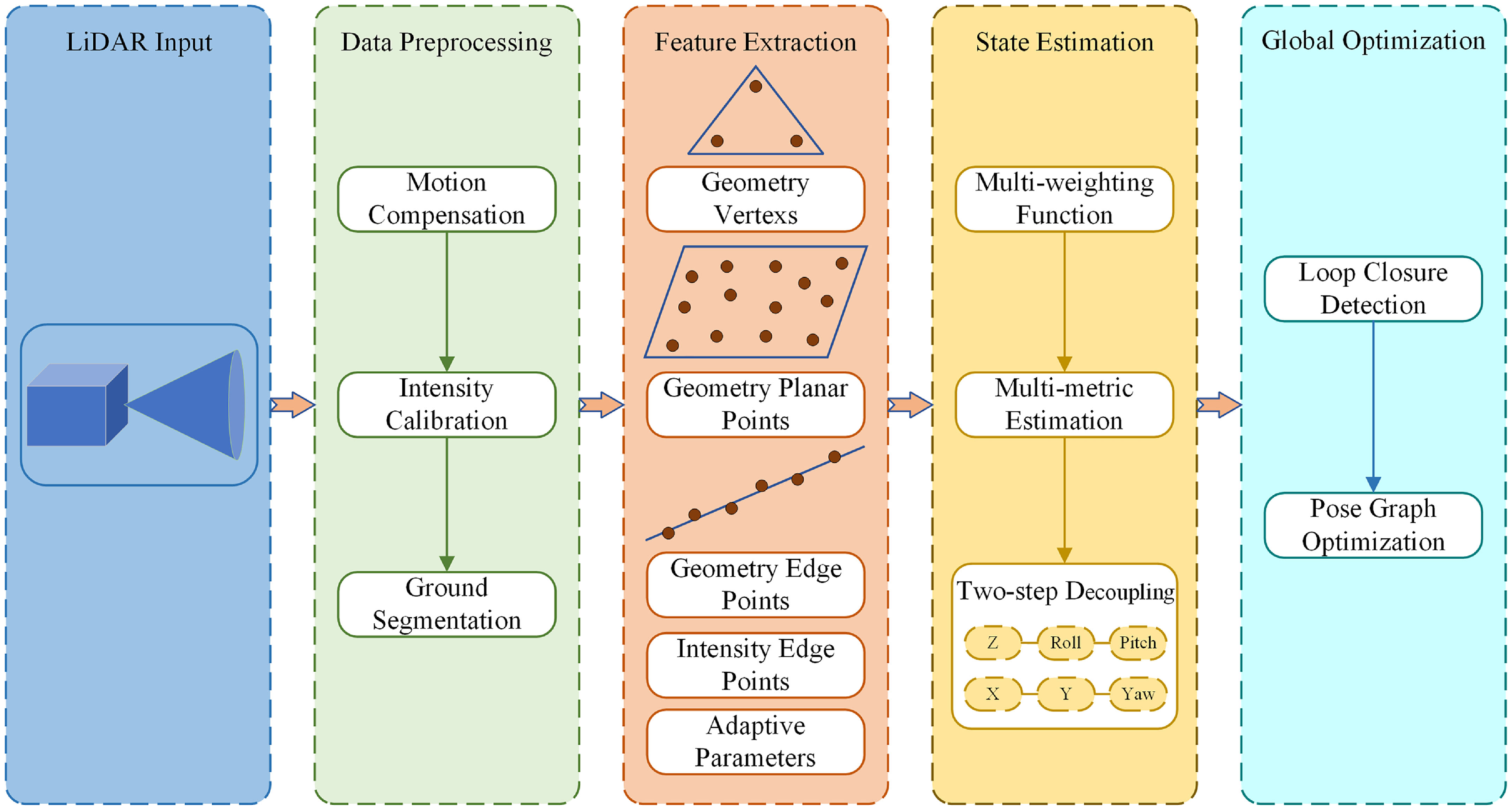
The pipeline of the proposed method is illustrated in Figure 1. The entire system consists of four parts: data preprocessing, feature extraction, state estimation, and global optimization. The preprocessing module performs motion distortion compensation for LiDAR frames, intensity data calibration, and ground point segmentation. The feature extraction module extracts multiple types of feature points from both geometric and intensity data. The state estimation module performs multi-metric registration of various extracted features coupled with a two-step decoupling strategy. Finally, the global optimization module executes loop closure detection and graph optimization.
Overview of our proposed system. Preprocessing is performed to compensate, correct, and separate the point cloud, followed by the adaptive extraction of multiple geometric features of vertices, edge points, and plane points, as well as intensity edge feature points. Subsequently, multi-metric feature matching and two-step decoupling are conducted, and finally, global optimization is performed.

3.1. Data preprocessing
3.1.1. Motion compensation
To address the motion distortion of point cloud frames, all points in the current or given frame are projected to either the start or end time of the frame. Assuming constant velocity motion within the frame, the transformation formula for projecting any point
 $\boldsymbol{p}_{i}$
to the frame’s end time is given by:
 \begin{equation} \boldsymbol{p}^{\prime}_{i}=\textit{slerp}\left(\boldsymbol{R}_{e},\boldsymbol{p}_{e},s\right)+\boldsymbol{t}_{e} \end{equation}
where
 $\textit{slerp}()$
is a spherical linear interpolation function,
 $\boldsymbol{p}_{e}$
is the endpoint,
 $\boldsymbol{R}_{e}$
and
 $\boldsymbol{t}_{e}$
are the overall rotation and translation parameters, and
 $s$
is the interpolation factor, representing the proportion of current time to overall time.
3.1.2. Intensity calibration
LiDAR intensity values are influenced by various factors, including incidence angle, measurement distance, and surface reflectivity. To maintain stable intensity measurements, intensity calibration is necessary to eliminate the effects of these external factors:
 \begin{align}& I=\eta \frac{\rho \cos \alpha }{r^{2}} \end{align}
 \begin{align}&\, \frac{I}{\cos \alpha }\propto \frac{\rho }{r^{2}} \end{align}
where
 $\eta$
is the constant set,
 $\rho$
is the reflectivity,
 $\alpha$
represents the incidence angle,
 $r$
represents distance returned from the measurement.
Therefore, the intensity measurement is primarily dependent on
 $\alpha$
, we utilize
 $I/\cos \alpha$
rather than
 $I$
as the intensity measurement value.
3.1.3. Ground segmentation
Use dual threshold filtering method for ground point segmentation. The method first projects the point cloud onto a horizontal reference surface and partitions it into 2D grids. A filtering threshold is then determined for each grid based on the minimum height within its 3 × 3 neighborhood grid region. For an arbitrary point
 $\boldsymbol{p}_{j}^{(i)}$
, the segmentation is formulated as:
 \begin{equation} \boldsymbol{p}_{j}^{\left(i\right)}\in \left\{\begin{array}{l} NG,\text{ if }h_{j}-h_{\min }^{\left(i\right)}\gt \delta _{1}\text{ or }h_{\min }^{\left(i\right)}-h_{\text{nmin }}^{\left(i\right)}\gt \delta _{2}\\[5pt] G,\text{otherwise } \end{array}\right. \end{equation}
where
 $h_{j}$
is the height of the current point,
 $h_{\min }^{(i)}$
and
 $h_{n\min }^{(i)}$
denote the minimum heights of the current grid and its neighborhood grids,
 $\delta _{1}$
and
 $\delta _{2}$
are two set thresholds,
 $NG$
and
 $G$
represent non-ground points and ground points, respectively.
3.2. Feature extraction
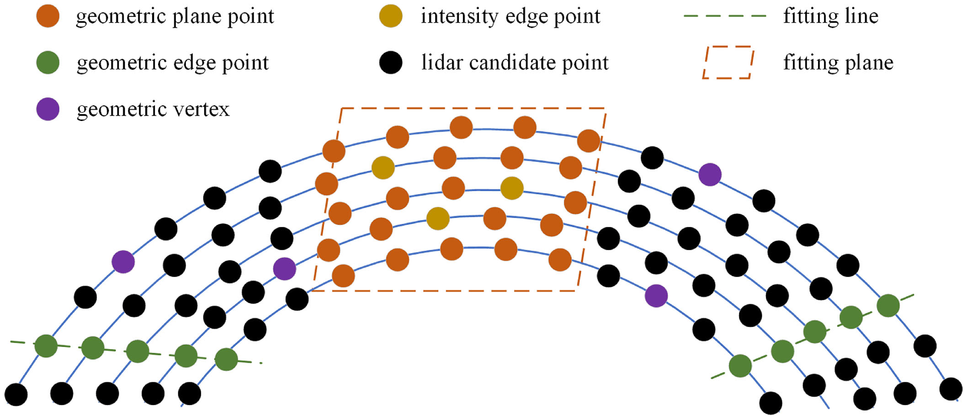
This section primarily focuses on extracting multiple types of geometric and intensity edge features, as illustrated in Figure 2. It begins with nearest neighbor search on the point cloud to cluster different types of points, followed by feature classification of the candidate points.
Schematic diagram of feature distribution and extraction. Using the nearest neighbor search strategy to search for adjacent points of different features, and then fitting the corresponding planes and lines.

3.2.1. Geometry feature extraction
Firstly, a voxel-based method is used to downsample the segmented non-ground point clouds to reduce point density, followed by the nearest neighbor search to ensure consistency in local point cloud distribution. After these preprocessing steps, PCA is employed to extract multiple geometric features. Specifically, within a defined neighborhood radius of the current point, we search for the nearest point set and compute its covariance matrix
 $\sum$
:
 \begin{equation} \begin{array}{l} \overline{\boldsymbol{u}}=\frac{1}{|{\textrm{N}}|}\sum _{i\in {\textrm{N}}}\boldsymbol{p}_{i}\\[5pt] \sum =\frac{1}{|{\textrm{N}}|}\sum _{i\in {\textrm{N}}}\left(\boldsymbol{p}_{i}-\overline{\boldsymbol{u}}\right)\left(\boldsymbol{p}_{i}-\overline{\boldsymbol{u}}\right)^{T} \end{array} \end{equation}
where
 $p_{i}$
and
 $\overline{u}$
respectively represent the i-th point and the mean of point set
 ${\textrm{N}}$
.
Using covariance matrix for eigenvalue decomposition to determine three eigenvalues and the corresponding eigenvectors:
 \begin{equation} \sum \boldsymbol{v}_{i}=\lambda _{i}\boldsymbol{v}_{i},\quad i=1,2,3 \end{equation}
where
 $\lambda _{1}\gt \lambda _{2}\gt \lambda _{3} , \boldsymbol{v}_{1}$
is the principal vector,
 $\boldsymbol{v}_{3}$
is the normal vector.
Then define local linearity
 $\sigma _{l}$
, planarity
 $\sigma _{p}$
and curvature
 $\sigma _{c}$
as:
 \begin{equation} \sigma _{l}=\frac{\lambda _{1}-\lambda _{2}}{\lambda _{1}},\quad \sigma _{p}=\frac{\lambda _{2}-\lambda _{3}}{\lambda _{1}},\quad \sigma _{c}=\frac{\lambda _{3}}{\lambda _{1}+\lambda _{2}+\lambda _{3}} \end{equation}
Based on the magnitude of local eigenvalues and the direction of eigenvectors, three types of feature points can be extracted: planar features, linear features, and vertex features. A point is classified as a linear feature point when the local linearity within its neighborhood exceeds a predefined threshold. Similarly, points are identified as planar features when their local planarity surpasses the threshold. Afterwards, vertex features are extracted from the remaining points through curvature sampling. For ground point clouds, which contain limited vertex and linear points, only planar features are extracted. The specific classification criteria are defined as follows:
 \begin{equation} \boldsymbol{p}_{i}\in \left\{\begin{array}{c} P,\text{ if }\sigma _{l}\gt \sigma _{lth}\\[5pt] L,\text{ if }\sigma _{p}\gt \sigma _{pth}\\[5pt] V,\text{ if }\sigma _{c}\gt \sigma _{cth} \end{array}\right. \end{equation}
where P, L, and V, respectively, represent planar points, linear points, and vertices,
 $\sigma _{lth}$
is the linear feature threshold,
 $\sigma _{pth}$
is the planar feature threshold,
 $\sigma _{cth}$
is the curvature threshold, also known as the vertex feature threshold.
3.2.2. Intensity feature extraction
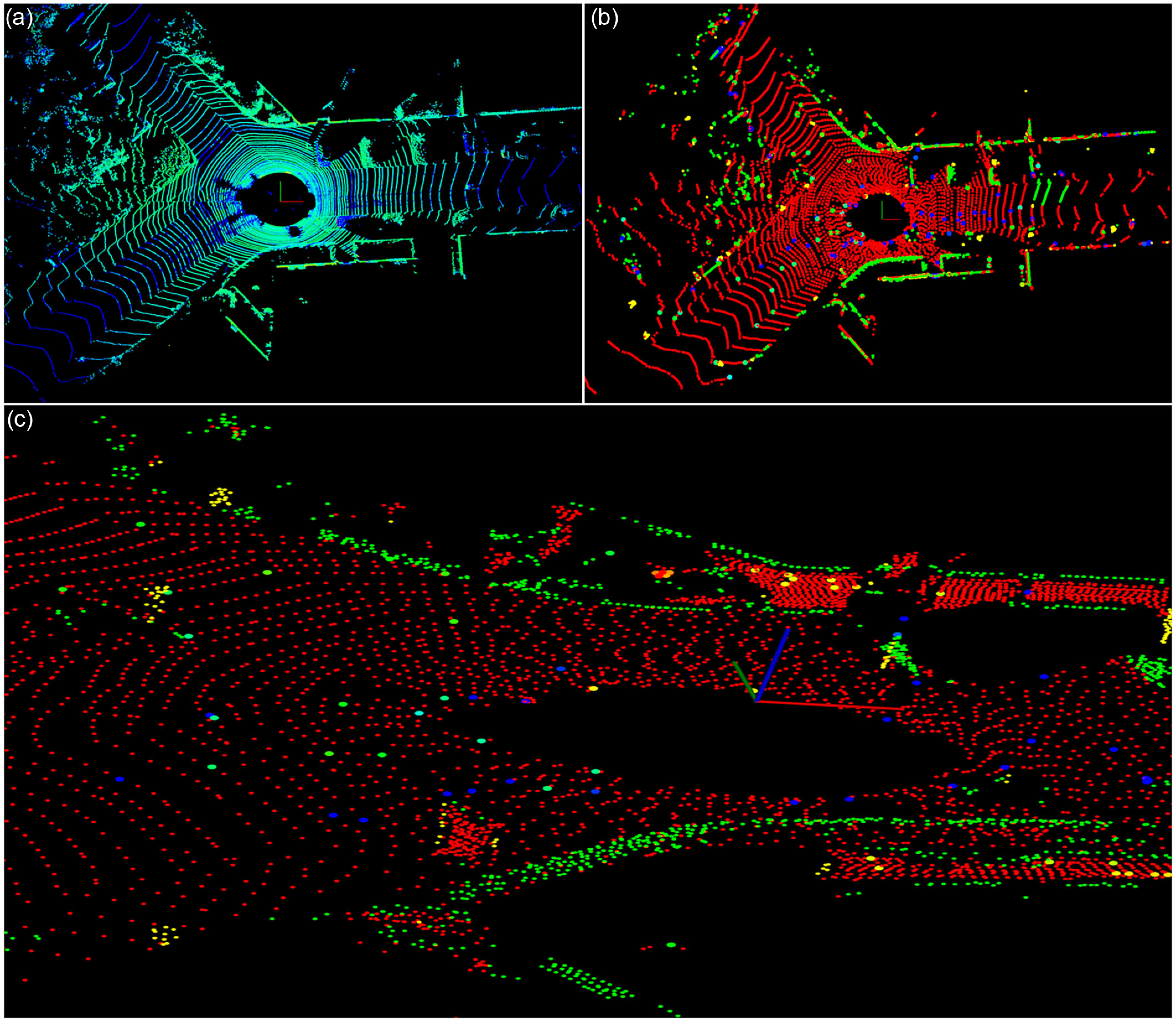
Unlike three-dimensional geometric features, intensity features are one-dimensional reflectance data from LiDAR measurements. Referring to similar methods in ref. [Reference Li, Ji, Liang, Ge and Yan31] and IGE-LIO [Reference Chen, Zhu, Yu, Jiang, Hua, Fu and Kuang34], we extract intensity edge features by identifying points with significant intensity variations within planar point clouds through intensity difference computation, as shown in Figure 3. Although intensity planar features can represent regions of identical material composition, their extraction is susceptible to noise and viewpoint changes. Therefore, we focus exclusively on extracting more salient intensity edge features. The intensity difference between two points is formulated as:
 \begin{equation} \Delta I=\left| \frac{\left\| \boldsymbol{p}_{i}\right\| _{2}^{2}\cdot \cos \left(\theta _{j}\right)}{\left\| \boldsymbol{p}_{j}\right\| _{2}^{2}\cdot \cos \left(\theta _{i}\right)}\tilde{I}_{i}-\tilde{I}_{j}\right| \end{equation}
where
 $\boldsymbol{p}_{i}$
and
 $\boldsymbol{p}_{j}$
are two candidate points,
 $\tilde{I}_{i}$
and
 $\tilde{I}_{j}$
are the corrected intensity values, and according to Eq. (3), the corrected intensity value
 $\tilde{I}$
is represented by
 $I/\cos \alpha$
.
 $\theta _{j}$
and
 $\theta _{j}$
are the incident angles, and the values of cosine represent the magnitude of the point in its normal vector direction, and the formula is:
 \begin{equation} \cos \left(\theta _{i}\right)=\frac{\left(\boldsymbol{p}_{i}\right)^{T}\cdot \overline{\boldsymbol{n}}_{i}}{\left\| \boldsymbol{p}_{i}\right\| _{2}} \end{equation}
where
 $\overline{\boldsymbol{n}}_{i}$
is the normal vector, and the formula definition for
 $\cos (\theta _{j})$
is the same.
Feature extraction of the current frame. (a) Original point cloud. (b) Extracted plane (red), edge (blue), vertices (purple), and intensity edge points (intensity color) feature points. (c) Enlarge the intensity edge points on the ground and display different intensity colors.

3.2.3. Adaptive parameter
In structured environments with rich geometric information, line and planar features alone can achieve high-precision localization. However, in degenerate scenarios with sparse features, additional constraints from point features and intensity features are necessary to achieve satisfactory performance. Inspired by [Reference Xu, Lin, Wang and Chen26], we propose an adaptive feature extraction strategy based on the distribution and quantity of geometric and intensity features, enhancing both algorithm responsiveness and environmental robustness.
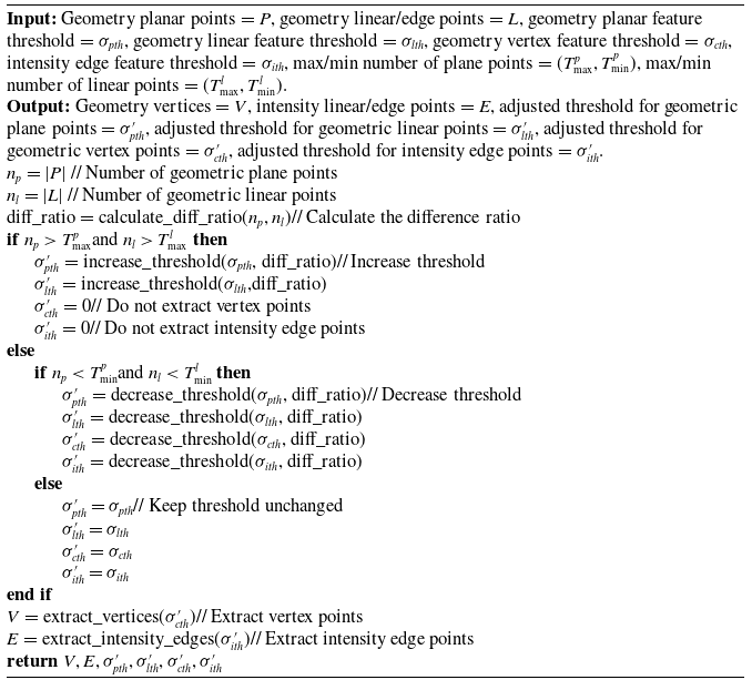
The basic principle of the adaptive parameter adjustment proposed by us for adaptive feature extraction is shown in Algorithm 1. It is mainly based on the number of geometric plane points and edge points to determine whether to extract geometric vertices and intensity edge points and adjust the threshold for feature extraction. If the number of geometric plane points and edge points exceeds the maximum threshold value, the environment is rich in geometric information. At this time, it is not necessary to extract geometric vertex and intensity edge point features, and the extraction threshold value is magnified according to the point data to extract more significant features. If it is less than the minimum threshold value, it is necessary to add geometric vertex and intensity edge point features, and reduce the relevant threshold value to extract more features. If the number of points is between the maximum and minimum, the default threshold parameter is used. The initial threshold parameters are set as follows:
 \begin{equation} \sigma _{lth}=0.65,\sigma _{pth}=0.65,\sigma _{cth}=0.12,\sigma _{ith}=0.20 \end{equation}
where
 $\sigma _{lth} , \sigma _{pth}$
and
 $\sigma _{cth}$
are defined by Eq. (8), and
 $\sigma _{ith}$
is the intensity edge threshold, which is related to Eq. (9).
Adaptive Parameter Adjustment

3.3. State estimation
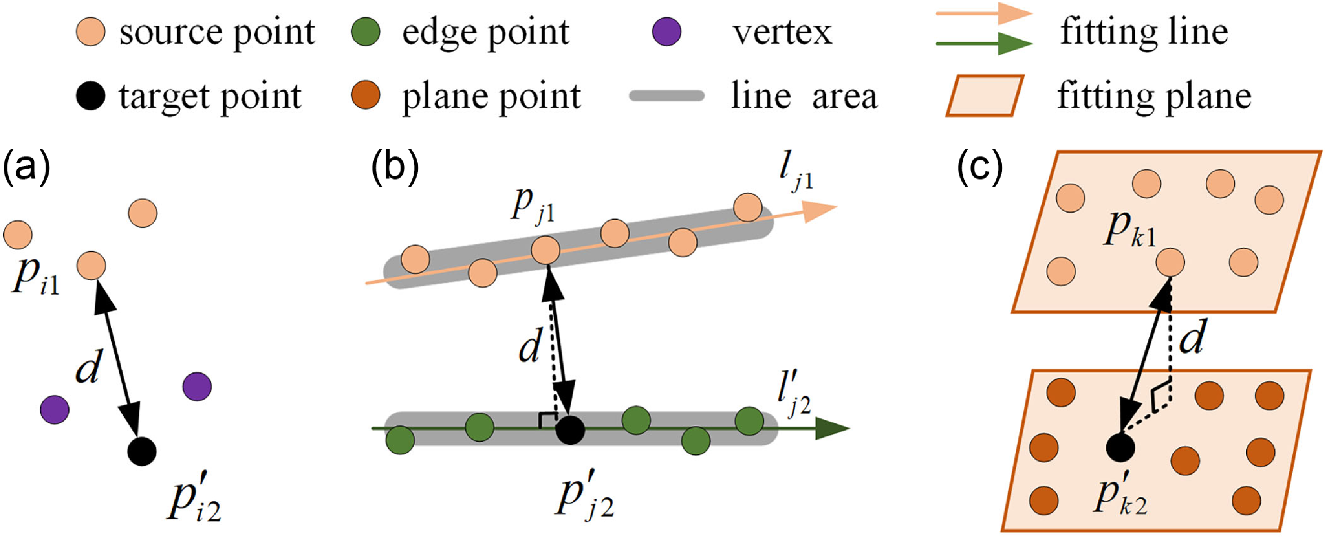
For each feature point in the source frame, corresponding feature points within a defined range are identified in the target frame using nearest neighbor search, as illustrated in Figure 4. For planar and linear features, directional consistency checking of normal vectors and principal directions is performed to enhance feature association accuracy. Under multi-feature correspondence, the multi-metric approach involves estimating the optimal pose transformation through three residual metrics: point-to-point, point-to-line, and point-to-plane distance residuals. The transformation estimation
 $\boldsymbol{T}$
is formulated as a multi-weighted optimization problem with the following objective function:
 \begin{equation} \boldsymbol{T}=\underset{\boldsymbol{T}}{\textit{argmin}}\left(\sum _{i}w_{i}f^{2}\left(d_{i}\right)+\sum _{j}w_{j}f^{2}\left(d_{j}\right)+\sum _{k}w_{k}f^{2}\left(d_{k}\right)\right) \end{equation}
where
 $w_{i} , w_{j}$
and
 $w_{k}$
denote the weight coefficients,
 $d_{i} , d_{j}$
and
 $d_{k}$
represent the residuals, and
 $f(d_{i}) , f(d_{j})$
and
 $f(d_{k})$
are the corresponding residual functions.
Schematic illustration of three different feature distance error metrics. (a) Point to point. (b) Point to line. (c) Point to plane. Different features of the target point are represented by different colors, with superscripts representing transformed points and vectors, and black double arrows representing corresponding feature distance error vectors.

3.3.1. Multi-weight function
To differentiate and balance the contribution and quality of each feature type in pose estimation, we propose a novel weight function based on residuals and feature characteristics. First, a robust kernel function incorporating M-estimators [Reference Guo, Borges, Park and Gawel35] is employed to penalize large residuals, and a scale parameter of 1 is adopted to enhance computational efficiency. The feature weight function based on residual weights
 $w_{i}^{\textrm{res}}$
is defined as:
 \begin{align} &w_{i}^{\textrm{res}}=\varepsilon \left(\varepsilon ^{2}+1\right)^{-\frac{1}{2}}\notag\\[5pt] &\varepsilon =\frac{f}{\sigma } \end{align}
where
 $f$
is the residual in Eq. (11),
 $\varepsilon$
is the normalized residual, and
 $\sigma$
is the threshold of noise.
For geometric planar features, both intensity values and smoothness contribute to feature quality. Therefore, the weight for geometric planar features can be expressed as:
 \begin{align} {l} &w_{i}^{GPP}=\frac{2.0}{2.0-e^{-2{\sigma _{I}}{c_{i}}}}\notag\\[5pt] &c_{i}=\frac{1}{\left| N\right| \cdot \left\| \textbf{p}_{i}\right\| }\left\| \sum _{p_{j}\in M ,i\neq j}\left(\textbf{p}_{i}-\textbf{p}_{j}\right)\right\| \end{align}
where
 $c_{i}$
is the smoothness of the point
 $\textbf{p}_{i}$
, and
 $\textbf{p}_{j}$
is the neighborhood point of
 $\textbf{p}_{i} , M$
is the set of points around
 $\textbf{p}_{j}$
, and
 $N$
is the number of points in the
 $M$
set, and
 $\sigma _{I}$
is the parameter of the Gaussian distribution of intensity values, which is described as:
 \begin{align} &\mu =\frac{1}{N}\sum _{j=1}^{N}I_{j}\notag\\[5pt] &\sigma _{I}^{2}=\frac{1}{N-1}\sum _{j=1}^{N}\left(I_{j}-\mu \right)^{2} \end{align}
where
 $I_{j}$
represents the intensity value of point j,
 $\mu$
is the average intensity of the point set, and
 $\sigma _{I}^{2}$
is its variance.
For geometric edge features, smoothness has a more significant impact; therefore, the weight is defined as:
 \begin{equation} w_{i}^{GEP}=\frac{2.0}{1.0-e^{-{c_{i}}}} \end{equation}
Similarly, the weight for geometric vertex features is defined as:
 \begin{equation} w_{i}^{GVP}=\frac{2.0}{1.0+e^{-{c_{i}}}} \end{equation}
The weight of intensity variations between vector points is defined as:
 \begin{equation} w_{i}^{IEP}=\frac{2.0}{1.0+e^{-{\unicode[Arial]{x0394}} I/255}} \end{equation}
where
 ${\unicode[Arial]{x0394}} I$
denotes the intensity difference.
Therefore, the final weight is:
 \begin{equation} w_{i}=w_{i}^{res}\times w_{f} \end{equation}
where
 $w_{f}=w_{i}^{GPP}\cdot w_{i}^{GEP}\cdot w_{i}^{GVP}\cdot w_{i}^{IEP}$
is the weight of various features. Similarly,
 $w_{j}$
and
 $w_{k}$
.
The larger the weight value of a feature point, the more representative it is, thereby improving the results of pose estimation.
3.3.2. Multi-metric estimation
Inspired by MULLS [Reference Pan, Xiao, He, Shao and Li23] and [Reference Xu, Lin, Wang and Chen26], the calculation formula for point-to-point, point-to-line, and point-to-plane error functions is:
 \begin{equation} \begin{array}{l} f\left(d_{i}\right)=\left\| \boldsymbol{p}_{i1}-\boldsymbol{T}\boldsymbol{p}^{\prime}_{i2}\right\| _{\sigma }\\[5pt] f\left(d_{j}\right)=\left\| \left(\boldsymbol{p}_{j1}-\boldsymbol{T}\boldsymbol{p}^{\prime}_{j2}\right)\times \boldsymbol{l}_{c}\right\| _{2}\\[5pt] f\left(d_{k}\right)=\left| \left(\boldsymbol{p}_{k1}-\boldsymbol{T}\boldsymbol{p}^{\prime}_{k2}\right)\times \boldsymbol{n}_{c}\right| \end{array} \end{equation}
where
 $\sigma =(\sum _{i1}+\boldsymbol{T}{\sum ^{'}}_{i2}\boldsymbol{T}^{T})^{-1} , \boldsymbol{p}$
is the corresponding feature point,
 $\boldsymbol{l}_{c} , \boldsymbol{n}_{c}$
and
 $\sum _{i}$
represent the direction vector, normal vector, and covariance matrix, respectively.
The final pose transformation
 $\boldsymbol{T}$
is estimated by minimizing geometric and intensity residuals:
 \begin{equation} \boldsymbol{T}=\underset{\boldsymbol{T}}{\textit{argmin}}\left(\begin{array}{l} \sum _{i}w_{i}\left(\left\| \boldsymbol{p}_{i1}-\boldsymbol{T}\boldsymbol{p}^{\prime}_{i2}\right\| _{\sigma }\right)^{2}+\sum _{j}w_{j}\left(\left\| \left(\boldsymbol{p}_{j1}-\boldsymbol{T}\boldsymbol{p}^{\prime}_{j2}\right)\times \boldsymbol{l}_{c}\right\| _{2}\right)^{2}+\\[5pt] \sum _{k}w_{k}\left(\left| \left(\boldsymbol{p}_{k1}-\boldsymbol{T}\boldsymbol{p}^{\prime}_{k2}\right)\times \boldsymbol{n}_{c}\right| \right)^{2} \end{array}\right) \end{equation}
3.3.3. Two-step decoupling
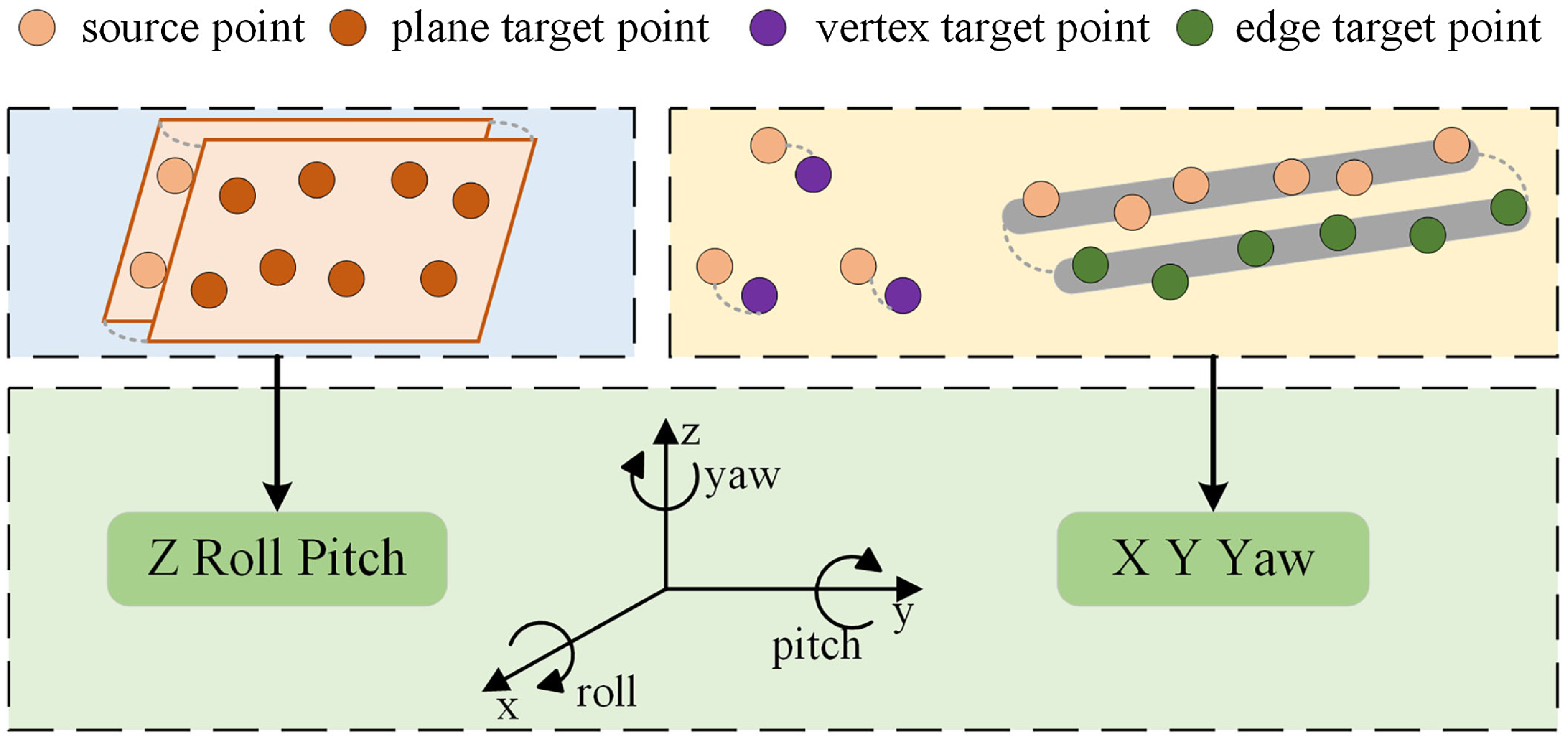
Inspired by LeGO-LOAM [Reference Shan and Englot21], the final pose transformation can be resolved through the two-step decoupled Levenberg-Marquardt (LM) method. As shown in Figure 5, the estimation of [Z, Roll, Pitch] is first performed using plane feature constraints, followed by the estimation of [X, Y, Yaw] using edge and vertex feature constraints. Finally, these are combined to obtain the six degrees of freedom pose estimation [X, Y, Z, Roll, Pitch, Yaw].
Schematic diagram of two-step decoupling for pose estimation. Plane feature point matching is used to estimate three pose variables, while vertex and edge feature point matching is used to estimate the other three pose variables.

3.4. Global optimization
Use TEASER [Reference Yang, Shi and Carlone36] based loop descriptors for loop detection. After completing loop detection and consistency verification, if there is a loop closure, perform pose graph optimization, correct the accumulated drift of the odometer, and finally output a dense global map.
4. Experiments and results
In this section, we conducted a series of qualitative and quantitative experiments on two public datasets to evaluate the proposed method, comprising unstructured environments that pose challenges for traditional LiDAR SLAM algorithms to manage, such as open highways, city streets, and so on.
4.1. Experimental setup
To ensure fairness and assess the computational cost of various methods, all algorithms in the public dataset were tested on desktop computers equipped with Intel i9-9900X 10-core CPU and 46 GB RAM. We employ two widely used SLAM error assessment metrics: Absolute Trajectory Error (ATE) and Relative Pose Error (RPE). Among them, RPE can be further divided into Relative Translation Error (RTE) and Relative Rotation Error (RRE). All the above indicators use their root mean square error (RMSE) data, and the relevant calculation formula [Reference Lu, Zhou, Wan, Hou and Song37] is as follows:
 \begin{equation} \begin{array}{l} \textrm{ATE}=\boldsymbol{Q}_{i}^{-1}\boldsymbol{S}\boldsymbol{P}_{i}\; \\[5pt] \textrm{RPE}=\left(\boldsymbol{Q}_{i}^{-1}\boldsymbol{Q}_{i+\Delta }\right)^{-1}\left(\boldsymbol{P}_{i}^{-1}\boldsymbol{P}_{i+\Delta }\right)\\[5pt] \text{RMSE}\left(ATE\right)=\left(\dfrac{1}{m}\sum _{i=1}^{m}\| \textit{trans}\left(ATE\right)\| ^{2}\right)^{1/2}\\[5pt] \text{RMSE}\left(ARE\right)=\left(\dfrac{1}{m}\sum _{i=1}^{m}\| rot\left(ATE\right)\| ^{2}\right)^{1/2}\\[5pt] \text{RMSE}\left(RTE\right)=\left(\dfrac{1}{m}\sum _{i=1}^{m}\| \textit{trans}\left(RPE\right)\| ^{2}\right)^{1/2}\\[5pt] \text{RMSE}\left(RRE\right)=\left(\dfrac{1}{m}\sum _{i=1}^{m}\| rot\left(RPE\right)\| ^{2}\right)^{1/2} \end{array} \end{equation}
where
 $\boldsymbol{P}_{i}\;$
and
 $\boldsymbol{Q}_{i}\;$
are the pose to be estimated and the pose truth,
 $\boldsymbol{S}$
is the transformation matrix,
 $i$
represents time, and
 $\Delta$
represents the fixed time difference of the interval.
4.2. Public datasets
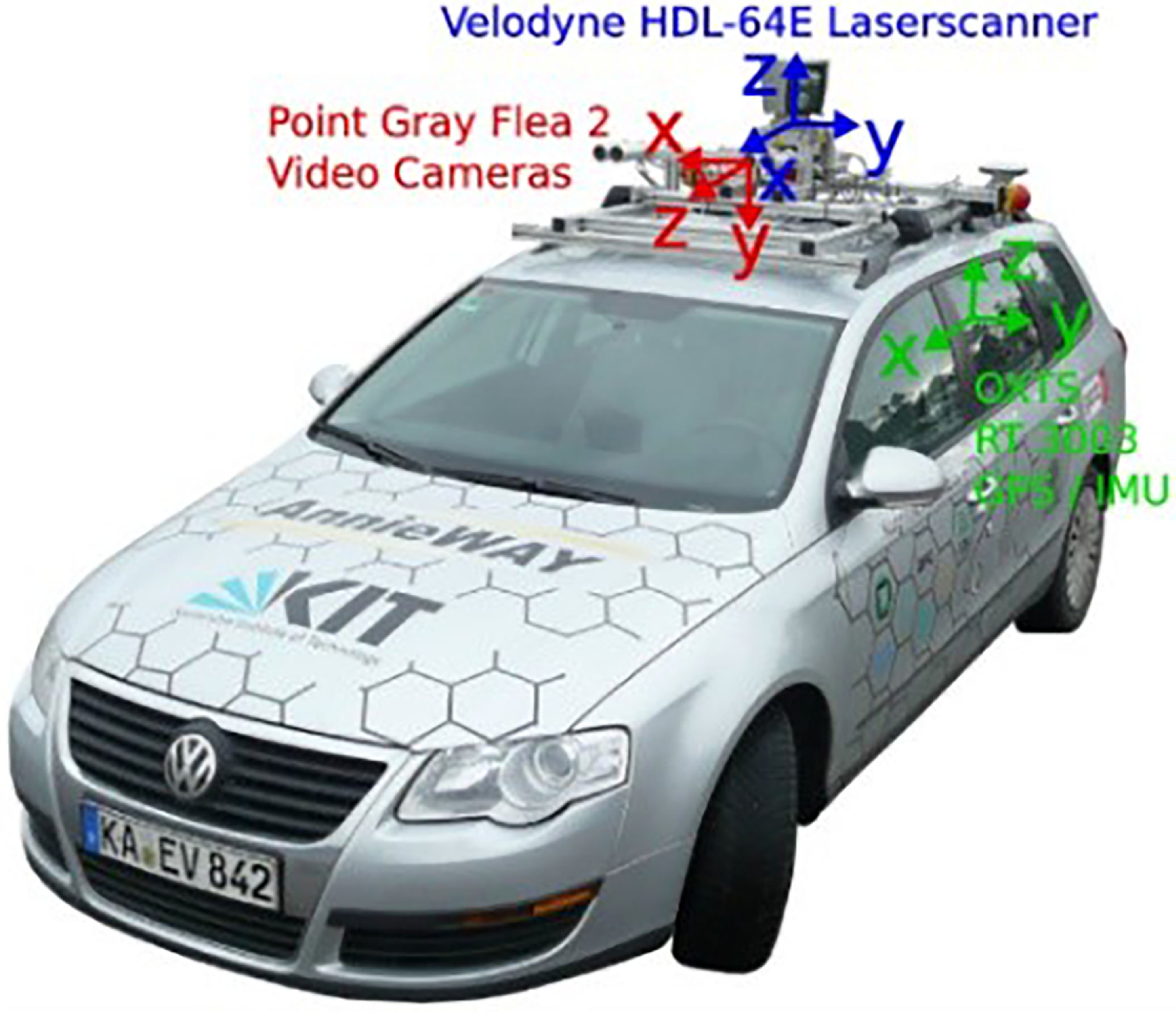
KITTI The KITTI dataset [Reference Geiger, Lenz and Urtasun38] is a publicly available dataset jointly created by the Karlsruhe Institute of Technology in Germany and the Toyota Technical Research Institute in the United States. It collects actual traffic scene data through fully equipped vehicles, as shown in Figure 6. It is a commonly used publicly available dataset for evaluating SLAM algorithms. HDL-64E LiDAR is utilized for data collection from 22 sequences in various scenarios, including urban, rural, and highway scenes, and provides 11 sequences with ground truth (00-10).
The data collection platform for the KITTI dataset. Including devices such as 3D LiDAR, cameras, IMU, and GPS, it can provide trajectory truth values for multiple sequences.

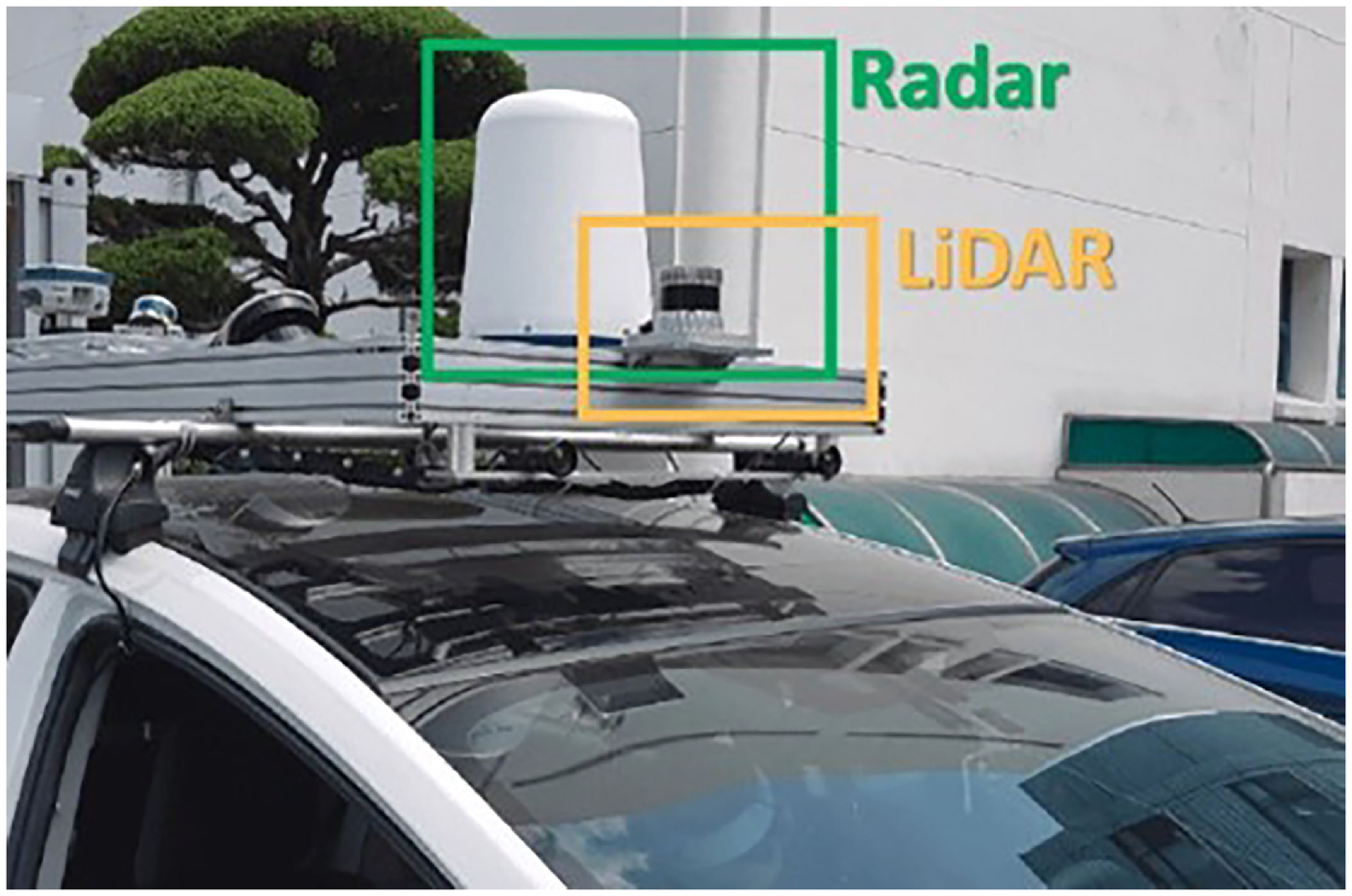
MulRan The MulRan dataset [Reference Kim, Park, Cho, Jeong and Kim39] is a multimodal dataset specifically designed for urban environments, collected using Radar and LiDAR sensors, as shown in Figure 7. This dataset collects four different environments, each of which has three subsequences. It also contains multi-session sequences of repeated tracks in the urban scene, and provides a six-dimensional real ground truth trajectory.
The data collection platform for the MulRan dataset. Equipped with a single radar and 3D LiDAR sensor, it can provide multi-mode distance measurement and trajectory truth.

4.3. Evaluation on public datasets
Quantitative experiments are conducted on both datasets, comparing our algorithm with basic and state-of-the-art pure geometric algorithms as well as intensity-assisted algorithms, including ALOAM,Footnote 1 LeGO-LOAM [Reference Shan and Englot21], MULLS [Reference Pan, Xiao, He, Shao and Li23], SC-LeGO-LOAM,Footnote 2 Intensity-SLAM [Reference Wang, Wang and Xie30], and ISC-LOAM [Reference Wang, Wang and Xie40].
4.3.1. Comparison with pure geometric algorithms
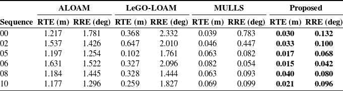
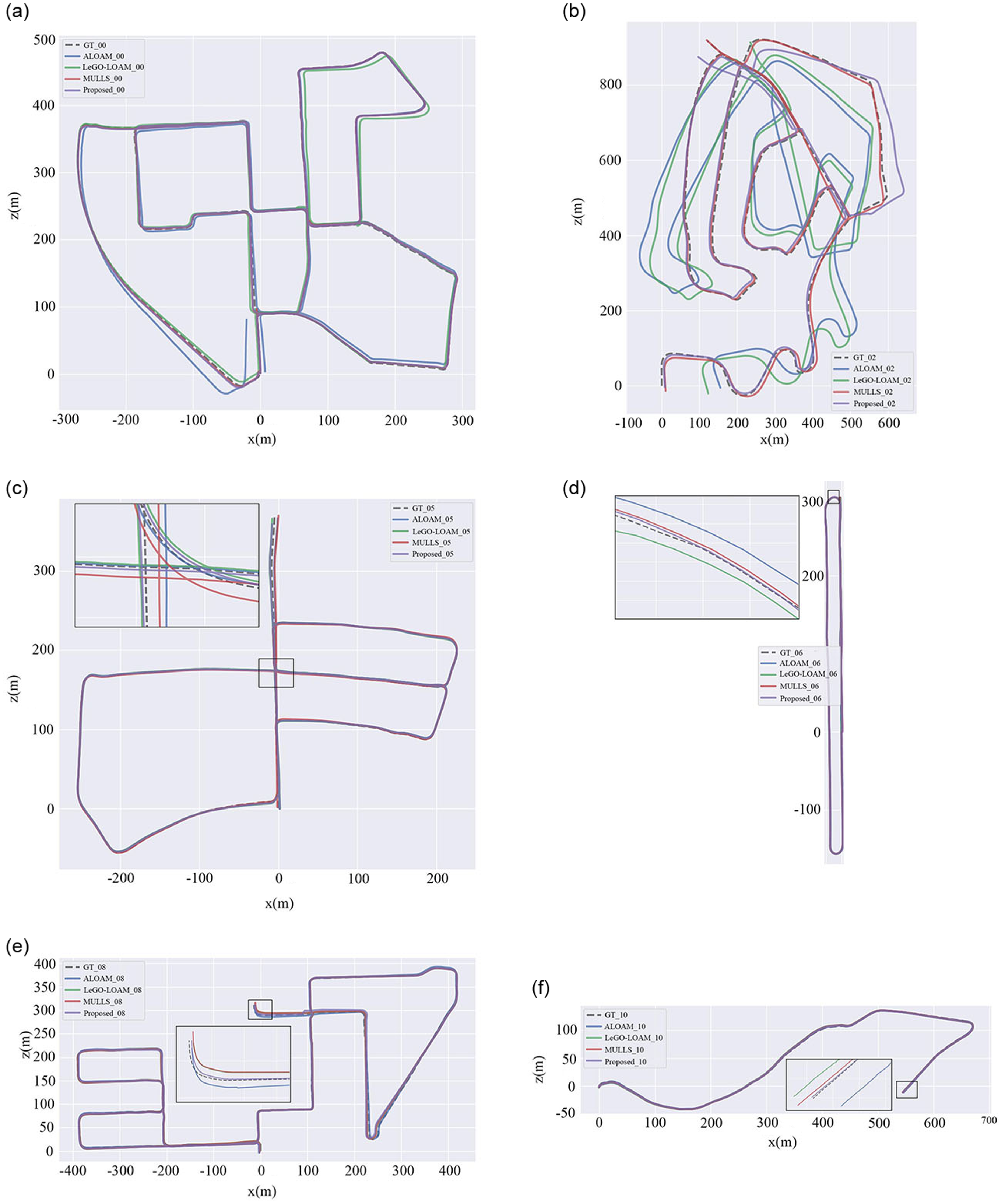
On the KITTI dataset, select sequences 00, 02, 03, 05, 07, and 09 are selected for the comparison of ATE, while select sequences 00, 02, 05, 06, 08, and 10 are chosen for the comparison of RTE and RRE, along with the corresponding trajectory plots. The comparisons are made with the pure geometric algorithms, and the results are presented in Table I, Table II, and Figure 8. The results indicate that in most sequences in the KITTI dataset, our proposed algorithm outperforms these three pure geometry algorithms in terms of accuracy. Specifically, in Table I, on the complex and comprehensive sequence 00, our odometry achieves an APE accuracy of 1.265 m, which is an improvement of 84.93% over ALOAM’s 8.392 m, 69.13% over LeGO-LOAM’s 4.098 m, and 28.93% over MULLS’ 1.780 m. Our method also shows enhanced accuracy compared to the other methods in the remaining sequences. In Table II, the relative pose accuracy shows that our proposed algorithm significantly outperforms the comparison algorithms. In the trajectory plot shown in Figure 8, our algorithm is closer to the ground truth, particularly in sparse scenarios such as turns and roads, indicating that our proposed algorithm has higher accuracy and robustness.
RMSE of ATE (m) comparison of pure geometric algorithms on KITTI dataset.

RMSE of RTE (m) and RRE (deg) comparison of pure geometric algorithms on KITTI dataset.

The estimated trajectory is compared with ALOAM, LeGO-LOAM, and MULLS on some KITTI dataset sequences, and their respective ground truths are also provided. (a) Seq 00. (b) Seq 02. (c) Seq 05. (d) Seq 06. (d) Seq 08. (f) Seq 10.

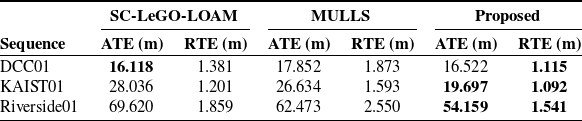
On the MulRan dataset, representative sequences DCC01, KAIST01, and Riverside01 are selected for algorithm comparison experiments. As shown in Table III, our algorithm outperforms both SC-LeGO-LOAM and MULLS in most of the two types of accuracy metrics, particularly in RTE, which demonstrates the effectiveness of our adaptive feature extraction and two-step decoupling.
4.3.2. Comparison with intensity-assisted algorithms
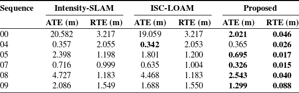
On the other hand, we select sequences 01, 04, 05, 07, 08, and 09 from the KITTI dataset to compare the ATE and RTE accuracy with state-of-the-art intensity-assisted algorithms, and the results are shown in Table IV. As shown in the table, our algorithm has demonstrated significantly superior accuracy in most sequences, especially with a more significant improvement in RTE accuracy, indicating the effectiveness of our algorithm. On the 04 sequence, our algorithm’s ATE is lower than these two types of algorithms because the sequence is a short linear path with a shorter running time. These three algorithms have similar ATE accuracy on this sequence, so RTE is more suitable for evaluating this sequence. Our algorithm has a more obvious high accuracy on RTE indicating that our algorithm still has superiority on this sequence.
4.3.3. Unstructured scenes mapping
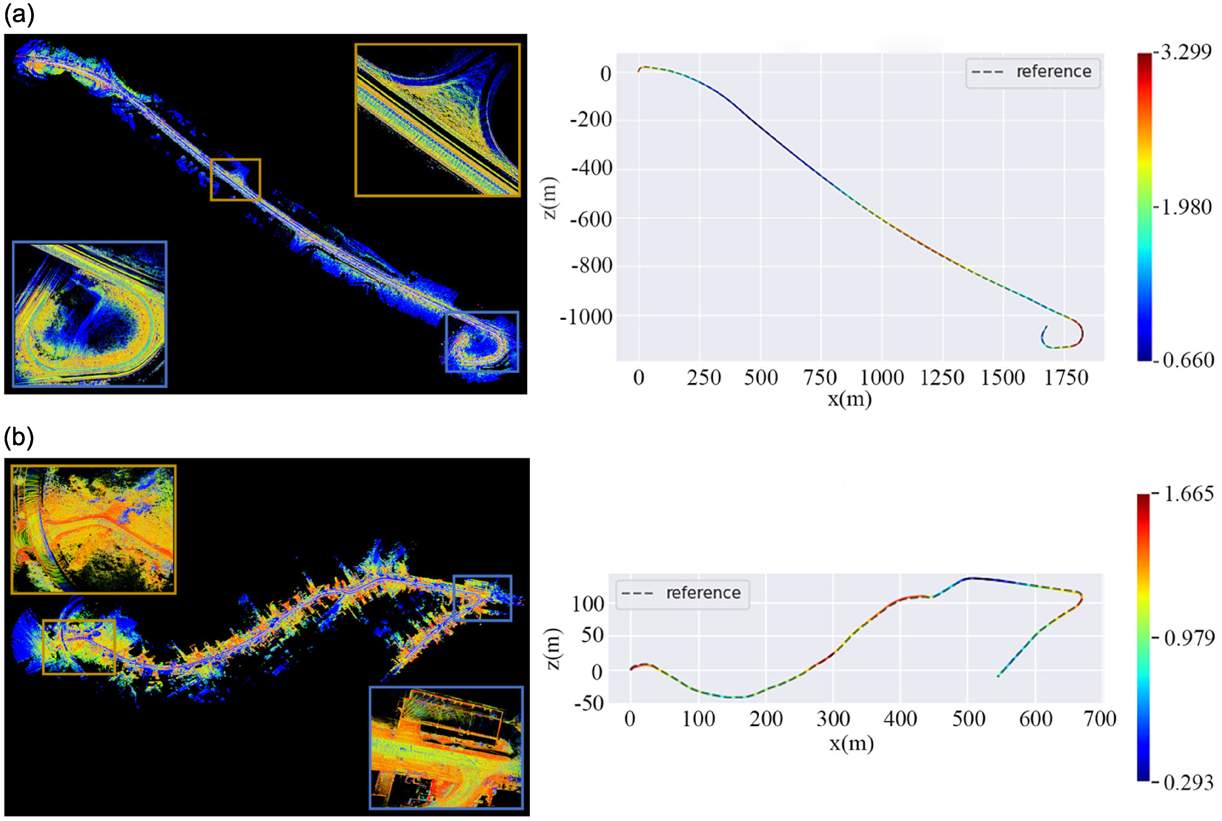
To illustrate the mapping performance of the algorithm we proposed in unstructured scenes with sparse features, we conducted qualitative and quantitative experiments on sequences 01 and 10 of the KITTI dataset containing unstructured features, as shown in Figure 9. It can be seen that even in challenging highway scenarios and small-town roads, our algorithm can establish accurate point maps with low drift poses.
RMSE of ATE (m) and RTE(m) comparison of geometric algorithms on MulRan dataset.

RMSE of ATE (m) and RTE(m) comparison of intensity-assisted algorithms on KITTI dataset.

Mapping and trajectory results of typical unstructured scenes. (a) KITTI-01 sequence is a highway scenario. (b) KITTI-10 sequence is an urban scenario.

4.4. Ablation study
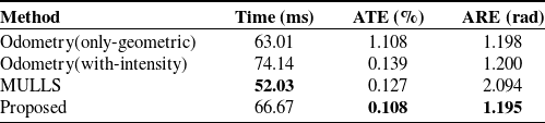
To analyze the performance of our proposed adaptive feature extraction method, we performed ablation experiments on odometer accuracy. Perform the localization accuracy experiment using the KITTI-05 sequence and compare it with pure geometry method, intensity odometry estimation method, and MULLS algorithm. There is no loop detection function used here, as shown in Table V. Although our proposed method increases some time consumption, the ATE error is 0.108% and the ARE error is 1.195 rad, which are better than other algorithms, indicating that our method is effective.
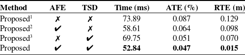
On the other hand, adaptive parameters and two-step decoupling are the focus of an ablation study conducted using the KITTI-07 sequence for experimentation, where loop closure detection functionality is used. For convenience, we use AFE to represent adaptive feature extraction and TSD to represent two-step decoupling. As shown in Table VI, Proposed1 does not use AFE or TSD, Proposed2 uses AFE but not TSD, and Proposed3 uses TSD but not AFE. From the results in the table, it can be seen that introducing these two methods significantly enhances both time efficiency and accuracy, particularly the incorporation of two-step decoupling, which greatly improves the accuracy of RTE.
4.5. Runtime analysis
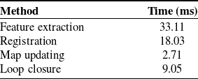
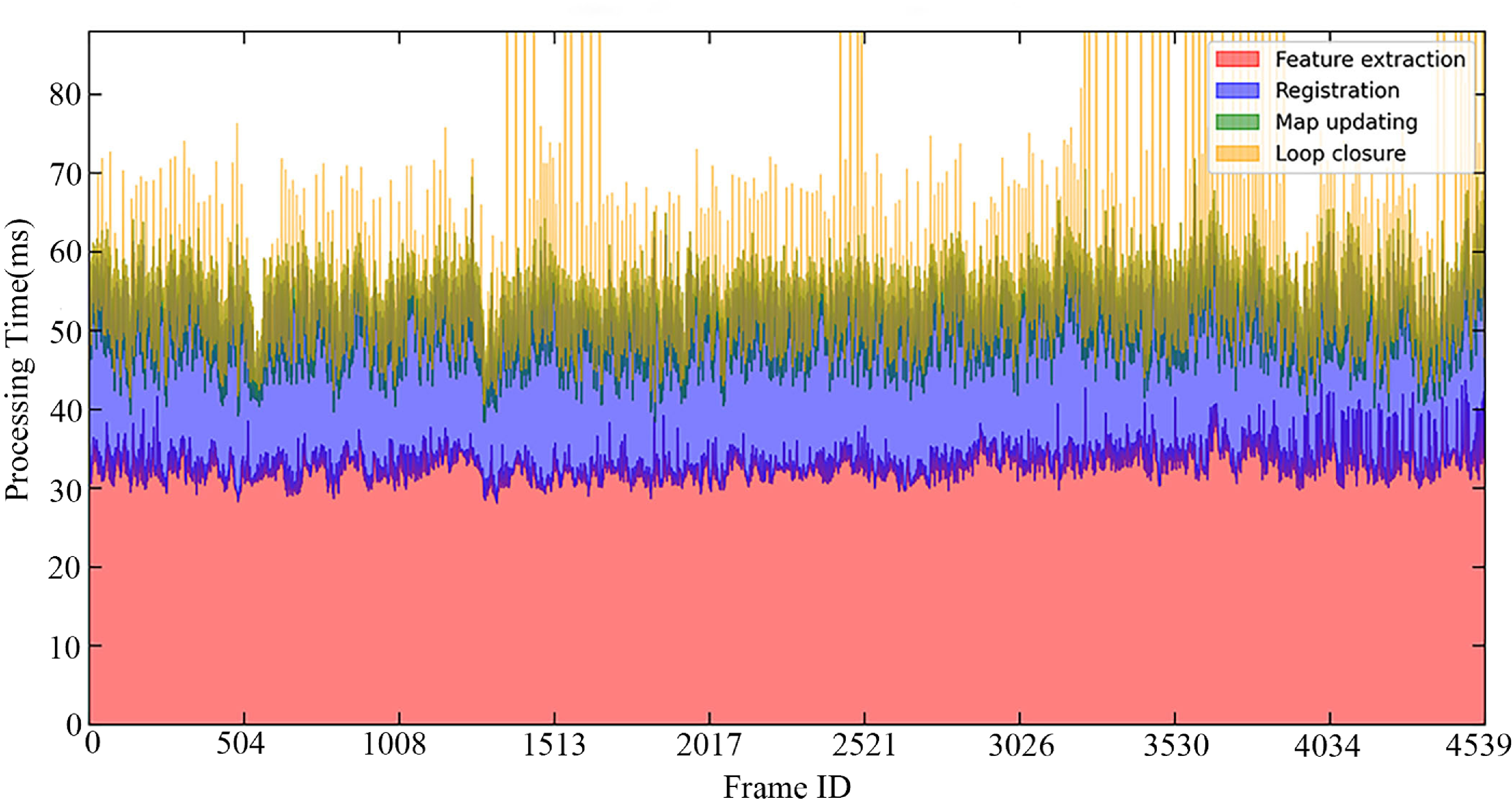
The detailed time consumption of the algorithm is presented in Table VII and Figure 10. In the KITTI-00 sequence, the feature extraction module has an average processing time of 33.11 ms per frame, the matching and registration module takes an average of 18.03 ms per frame, the map update module averages 2.71 ms per frame, and the loop closure detection module averages 9.05 ms per frame. Overall, our algorithm takes an average of 62.9 ms per frame, which meets the requirement for a LiDAR operating frequency of 10 Hz.
4.6. Validation on practical robot
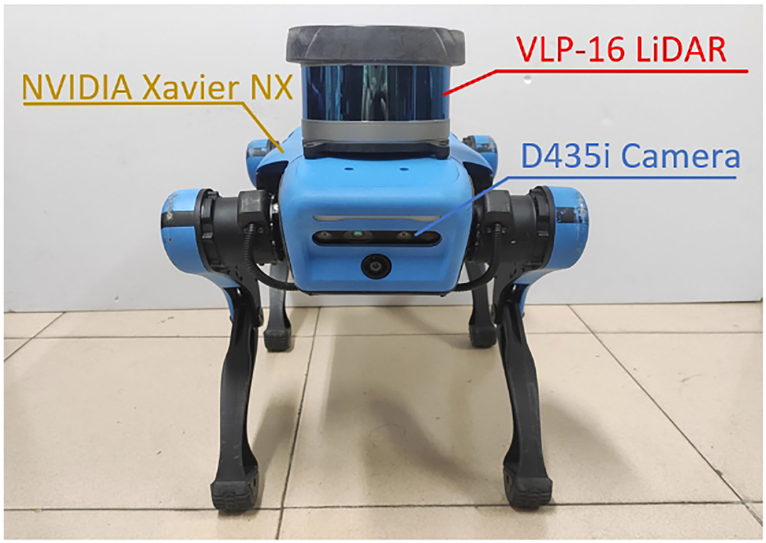
To assess the effectiveness of our proposed algorithm in actual unstructured environments, we performed qualitative tests using the Jueying Lite2 quadruped robot in the university park, as shown in Figure 11. The robot has a 3D LiDAR with VLP-16, a D435i depth camera, and an NVIDIA Jetson Xavier NX GPU processor, which effectively processes the measurement data.
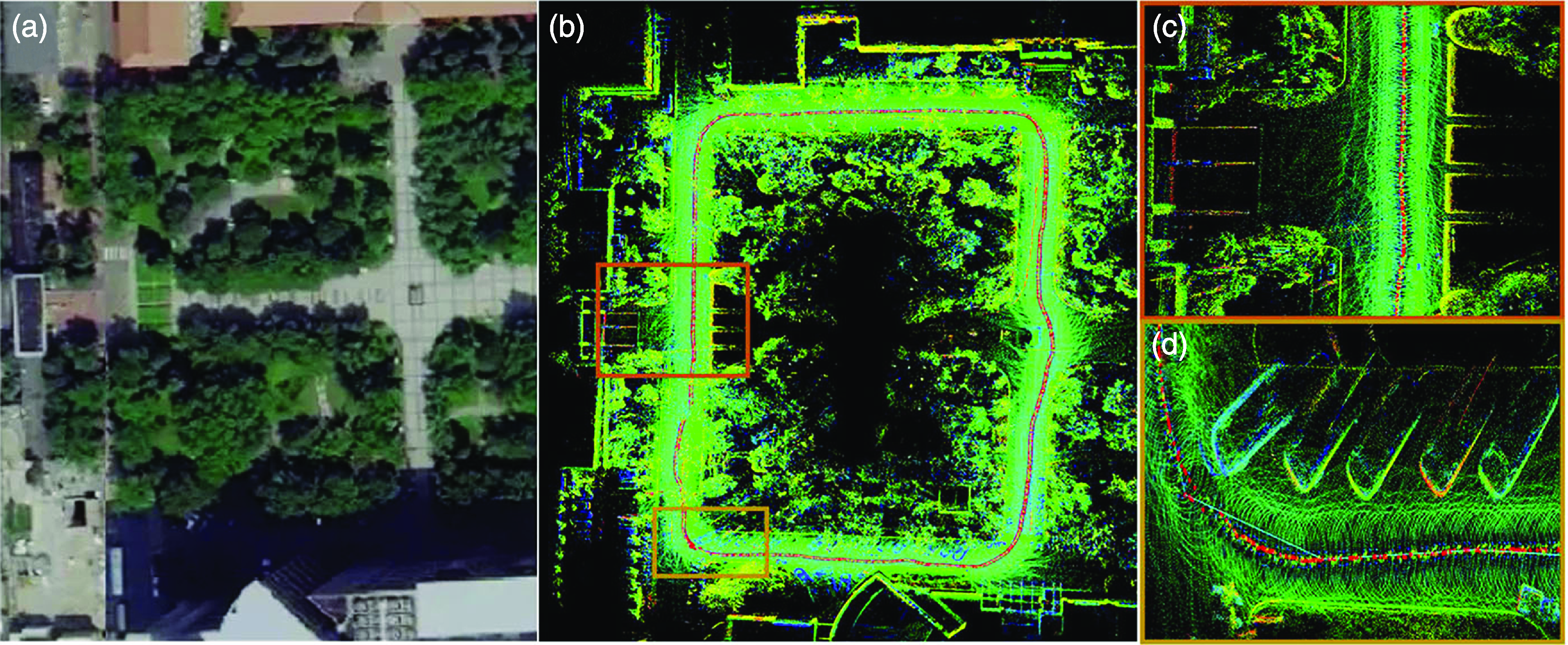
Figure 12(a) shows a segment of the actual scene captured on Gaode Map. Figure 12(b) displays the final dense mapping result, with the robot’s trajectory represented by red dots. The overall results are consistent with the actual scene, and the trajectory is very continuous, showing no significant drift.
The time and accuracy of odometer experiments.

The time and accuracy of ablation experiments.

Time consumption per frame for each module.

The running time per frame of each module in the proposed algorithm.

Figures 12(c) and (d) present enlarged local mapping results, where the object contours in the local mapping are also quite clear, without blurriness or ghosting. Therefore, the proposed method can accurately localize and construct dense maps in such unstructured scenarios.
5. Conclusion
In this paper, we propose a novel multi-metric LiDAR SLAM system that effectively addresses challenges in unstructured environments while achieving high localization accuracy. By adaptively extracting various types of geometric features and prominent intensity edge features, we enhance the capability to capture environmental information. We then perform multi-metric error calculations for point, line, and plane features, and design a new multi-weight function while employing a two-step decoupling strategy for pose variables to improve localization accuracy. Experimental results on various datasets with unstructured scenes demonstrate that our proposed algorithm achieves superior accuracy and real-time performance compared to state-of-the-art pure geometric and intensity-assisted algorithms. Compared with the benchmark algorithm, our proposed algorithm has improved ATE accuracy by 28.93% and real-time performance can reach 62.9 ms per frame. In future work, we intend to utilize other sensors for data fusion to further enhance the adaptability of our algorithm in intricate environments.
The Jueying Lite2 quadruped platform. It is equipped with a VLP-16 LiDAR, a D435i camera, and an NVIDIA Xavier NX processor.

Mapping in real unstructured campus scenes. (a) Aerial view of a real scene. (b) Algorithm mapping results. (c) and (d) are enlarged partial views.

Author contributions
All authors participated in the implementation of this study. The initial version of the manuscript was written by Xu Zhenghui, with Li Jian and Tang Ling providing assistance with experimental design, Wei Shimin and Chen Huanlong providing equipment, and all authors providing feedback on the early drafts of the manuscript. All authors have reviewed and approved the final manuscript.
Financial support
This work was supported by the funding from the Shanghai Institute of Aerospace Systems Engineering (No. SAST2022-015).
Competing interests
The authors declare that they have no conflicts of interest to disclose.
Ethical approval
None.