1. Introduction
Particle motion and orientation in viscoelastic (non-Newtonian) fluids arise ubiquitously in both natural and engineering systems. In the processing of fibre-reinforced polymers and rubbers, for example, the evolving orientation and spatial distribution of anisotropic fillers directly determine the macroscopic stress and the resulting mechanical anisotropy (D’Avino et al. Reference D’Avino, Greco and Maffettone2015; Ngo et al. Reference Ngo, Nguyen and Oh2021). Similar issues also arise in biological flows: in blood and other biofluids, the lateral distribution and alignment of cells influence transport, margination and the effective rheology (Ye et al. Reference Ye, Phan-Thien and Lim2016; Go et al. Reference Go, Byeon and Lee2017; Atwell et al. Reference Atwell, Badens, Charrier, Helfer and Viallat2022; Gürbüz et al. Reference Gürbüz, Pak, Taylor, Sivaselvan and Sachs2023; Recktenwald et al. Reference Recktenwald, Rashidi, Graham, Arratia, Del Giudice and Wagner2024). At the microscale, viscoelastic microfluidic systems further exploit particle–fluid interactions to achieve passive focusing, separation and sorting without the need for external fields (Del Giudice Reference Del Giudice2019; Zhou & Papautsky Reference Zhou and Papautsky2020; Kang et al. Reference Kang, Cha, Nguyen, Li, Klimenko, Zhang and Yuan2025). Underlying these phenomena is the fact that unlike Newtonian liquids, viscoelastic fluids exhibit stress relaxation, elastic memory and normal-stress differences (Larson Reference Larson1992; Sánchez et al. Reference Sánchez, Jovanović, Kumar, Morozov, Shankar, Subramanian and Wilson2022). Even in the weak-inertia limit, these properties can generate transverse forces and torques on suspended particles, thereby making a mechanistic understanding of particle migration and rotation essential for both microstructural modelling and device design.
In a shear flow, the cross-stream migration of particles is a deterministic phenomenon arising from hydrodynamic asymmetry around the particle, and is driven by well-defined lift mechanisms. In Newtonian fluids, classical analyses of lateral migration have mainly been developed for bounded or non-uniform shear fields, where the competition between shear-gradient and wall-induced lift provides a useful benchmark (Ho & Leal Reference Ho and Leal1976; Cherukat & McLaughlin Reference Cherukat and McLaughlin1994; Asmolov Reference Asmolov1999). The shear-gradient lift arises from asymmetric pressure distributions caused by velocity curvature, driving particles towards high-shear regions. In contrast, the wall-induced lift results from increased lubrication pressure in the near-wall region, pushing particles away from the wall. The balance between these two forces determines the final equilibrium position (Martel & Toner Reference Martel and Toner2014). More directly relevant to the present study, however, linear or confined shear flows do not possess the strong base-flow curvature characteristic of Poiseuille flow; rather, the lateral dynamics is determined by the combined effects of wall interactions, asymmetries in the particle-induced disturbance field, and fluid inertia when present. It has been shown that coupling between particle rotation and the local velocity-gradient field modifies the disturbance flow and pressure distribution around the particle, thereby generating lateral forces that drive cross-stream migration. More importantly, three-dimensional simulations and experiments have demonstrated viscoelasticity-induced cross-stream migration of a single rigid sphere in confined and planar shear flows, and quantified the effects of confinement, imposed shear rate and fluid normal stresses on the migration trajectories (D’Avino et al. Reference D’Avino, Maffettone, Greco and Hulsen2010; Caserta et al. Reference Caserta, D’Avino, Greco, Guido and Maffettone2011). Using three-dimensional finite-element simulations, D’Avino et al. (Reference D’Avino, Hulsen, Snijkers, Vermant, Greco and Maffettone2008) examined the rotation of a torque-free sphere in simple shear for 0 ≤ De ≤ 2.50, comparing Maxwell, Bird–Carreau, PTT (ε = 0.1 and 0.5) and Giesekus (α = 0.2 and 0.4) constitutive models, and showed that the rotation period increases with elasticity, while its transient evolution closely follows the build up of the first normal-stress difference. Complementary experiments by Snijkers et al. (Reference Snijkers, D’Avino, Maffettone, Greco, Hulsen and Vermant2009, Reference Snijkers, D’Avino, Maffettone, Greco, Hulsen and Vermant2011) tracked polystyrene and glass spheres of diameter 50–200 μm in several model viscoelastic fluids over shear-rate windows 0.23–0.84 s−1 (Boger fluid), 0.032–6.1 s−1 (shear-thinning polymer solution) and 0.56–1.1 s−1 (worm-like micellar solution), and showed that the dimensionless angular velocity collapses onto a single master curve when plotted against the Weissenberg number. In the same shear-flow setting, studies of a freely rotating sphere further showed that viscoelasticity slows particle rotation relative to the Newtonian case, with the reduction being governed primarily by normal-stress effects and scaling well with the Weissenberg number. In contrast, in viscoelastic fluids, particle migration is predominantly governed by the elastic lift force. The generation of elastic lift is closely associated with the spatial non-uniformity of the first normal-stress difference
N
1 =
 $ \boldsymbol{\tau} $
11−
 $ \boldsymbol{\tau} $
22 (where
 $ \boldsymbol{\tau} $
11 and
 $ \boldsymbol{\tau} $
22 are the streamwise and shear-gradient components of the polymeric stress tensor). More quantitatively, Naillon et al. (Reference Naillon, de Loubens, Chèvremont, Rouze, Leonetti and Bodiguel2019) measured migration in weakly elastic Poiseuille flows for Wi ≈ 10−2–10−1 and particle confinement ratios β = 0.1 and 0.2, and showed that the transverse migration velocity follows the scaling V
m
∝ Wi β
2, consistent with weakly elastic Oldroyd-B predictions. Overall, in viscoelastic fluids, elastic lift can dominate inertial contributions and drive robust cross-stream migration even at weak or moderate inertia. In channel geometries, this often leads to centreline focusing, sometimes termed the inverse Segré–Silberberg scenario, but in linear shear flow it is more useful to interpret the migration in terms of the coupling among normal-stress imbalance, wall interaction and particle rotation (Del Giudice et al. Reference Del Giudice, D’Avino, Greco, Netti and Maffettone2015; Del Giudice Reference Del Giudice2019; D’Avino Reference D’Avino2021).
Particle shape introduces additional complexity because drag, torque and the stresslet depend on orientation and aspect ratio. In a Newtonian unbounded simple shear and in the Stokes limit, an ellipsoid follows Jeffery orbits with an orbit constant set by the initial condition (Jeffery Reference Jeffery1922; Einarsson et al. Reference Einarsson, Candelier, Lundell, Angilella and Mehlig2015), while inertia, boundaries or non-Newtonian stresses can break this degeneracy and select long-time attractors. For spheroids in Couette flow, the coupling between particle rotation and the local velocity-gradient field modifies the surface-stress asymmetry, and can affect lateral drift when symmetry is broken (Huang et al. Reference Huang, Yang, Krafczyk and Lu2012). In viscoelastic suspending fluids, microstructural stresses further alter both the rotational dynamics and any resulting transverse motion. For dilute suspensions of spheroids in unconfined viscoelastic shear, rheological modelling and simulations quantified elasticity-induced changes in particle stresslets and effective material response (D’Avino et al. Reference D’Avino, Greco and Maffettone2015). At finite Reynolds number, prolate spheroids in viscoelastic shear can exhibit elasticity- and inertia-dependent rotational modes (Li et al. Reference Li, Xu and Zhao2023; Cui et al. Reference Cui, Jiang, Qiu and Zhao2025). Under confinement, viscoelastic normal stresses can drive levitation/migration of spheres in shear (Liu et al. Reference Liu, Lin, Ku and Yu2019; Su et al. Reference Su, Castillo, Pak, Zhu and Zenit2022), whereas in elasto-inertial duct/channel flows, non-spherical particles may display multiple rotational states and orientation-dependent migration (Hu et al. Reference Hu, Lin, Zhu, Yu, Lin and Li2024; Li et al. Reference Li, Xu and Zhao2024; Tanriverdi et al. Reference Tanriverdi, Cruz, Habibi, Amini, Costa, Lundell, Mårtensson, Brandt, Tammisola and Russom2024). Recent particle-resolved simulations by Hu et al. (Reference Hu, Lin, Zhu, Yu, Lin and Li2024) further mapped the elasto-inertial dynamics of spheroids in Oldroyd-B square-channel flow over 1 ≤ Re ≤ 100, 0 ≤ Wi ≤ 2 and 0.4 ≤ α ≤ 3, identifying four equilibrium-position families, and six rotational states for prolate spheroids, but five for oblate ones. It is worth noting that viscoelastic secondary flows in non-circular ducts are primarily associated with the second normal-stress difference N 2, and require constitutive models with non-zero N 2 (Giesekus-type fluids) (Yue et al. Reference Yue, Dooley and Feng2008). Despite these advances, a systematic understanding of the coupled migration and orientational dynamics of oblate spheroids in viscoelastic linear shear remains limited. Motivated by these observations, the present work employs three-dimensional direct-forcing (DF) fictitious-domain (FD) simulations to systematically investigate the cross-stream migration and rotational behaviour of oblate spheroidal particles in Oldroyd-B shear flows, with particular emphasis on the evolution of angular velocity along the migration path.
The structure of this paper is as follows. Section 2 presents the numerical model, including flow parameters, numerical methods and validation. Section 3 reports and discusses the migration behaviours of spherical and oblate particles under various fluid conditions. Section 4 summarises the main conclusions.
(a) Spherical particle and oblate particle in planar shear flow confined between parallel walls. (b) Particle coordinate system and surface Lagrangian points. (c) Oblate particle coordinate system and surface Lagrangian points. Here, a is particle radius, H is channel height, and L is channel length.

Figure 1. Long description
Panel A: A 3D diagram showing spherical and oblate particles in planar shear flow between parallel walls. The diagram includes labels for particle radius (a), channel height (H), and channel length (L). Arrows indicate the direction of fluid flow (U0). Panel B: A spherical coordinate system with labeled axes (x0, y0, z0) and surface Lagrangian points. Panel C: An oblate particle coordinate system with labeled axes (x0, y0, z0) and surface Lagrangian points, including angles (φ, θ).
2. Numerical model
2.1. Simulation set-up
Figure 1(a) illustrates the fluid–particle interactions and cross-stream migration of a single spherical and single oblate spheroidal particle in a bounded simple-shear Oldroyd-B flow. A Cartesian coordinate system is adopted, with the origin located on the channel centreline, and periodic boundary conditions are applied in both the axial (x) and streamwise (z) directions. The top and bottom walls are positioned at y = H/2 and y = –H/2, and move at velocities U 0 and -U 0 along the z-direction, thereby generating a linear shear with rate G = 2U 0/H, corresponding to a simple shear flow in the channel. Initially, both the fluid and the particle are at rest. The motion of the upper and lower walls subsequently generates the shear flow and accelerates the particle. The spherical particle has radius a, and the oblate particle is defined to have the same volume as a sphere of radius 0.75a. The oblate particle is described as x 0 2/a 0 2+ y 0 2/b 0 2+ z 0 2/c 0 2 = 1, where a 0, b 0 and c 0 denote the lengths of three semi-axes of the particles (a 0 = b 0). The oblate particle with AR = c 0/a 0 = 1/3 is initialised in two distinct orientations, represented in Euler-angle form as n p1 = (0, 0, 0) and n p2 = (π/2, π/4, π/2). The distributions of Lagrangian points on the particle surfaces are shown in figures 1(b) and 1(c). The particle is initially released at y 0 = −0.1H. The blockage ratio is defined as β = 2a/H. The particle is free to translate and rotate, with all six degrees of freedom retained in the simulations. The particle’s translational velocity and angular velocity are represented by the vectors U (V x , V y , V z ) and W p (ω x , ω y , ω z ), respectively. Here, x, y and z denote the fixed laboratory (inertial) coordinate system, while the components of W p are expressed in the particle-fixed (body) coordinate system attached to the particle principal axes.
2.2. The DF/FD method
This subsection presents the governing equations and outlines the numerical framework based on the FD method, which is used to simulate the migration behaviour of spherical and oblate particles in Oldroyd-B shear flows. This approach builds on the distributed Lagrange multiplier/FD technique reported by Glowinski et al. (Reference Glowinski, Pan, Hesla and Joseph1999), in which the particle interior is treated as a fictitious fluid, and rigid-body motion is enforced through a Lagrange multiplier. We dissociated the equations into three subproblems using a staggered time-stepping approach following the methods of Yu et al. (Reference Yu, Wang, Lin and Hu2019): fluid, particle and constitutive. The fluid subproblem involved solving Navier–Stokes equations with a finite-difference projection method on a uniform staggered grid using a fast Fourier transform based Poisson solver for pressure and second-order centred differencing for spatial derivatives. The particle subproblem maps velocities from Eulerian to Lagrangian nodes, and transfers the corresponding fictitious body forces back to the Eulerian grid via δ-functions approximated by trilinear interpolation. The flow variables are defined on a fixed Eulerian grid, whereas the particle is represented by Lagrangian collocation points at which the rigid-body constraint is imposed. Following Yu & Shao (Reference Yu and Shao2007), a discrete delta function is used to transfer quantities between the two grids, allowing the predicted velocity to be interpolated to the Lagrangian points, and the resulting constraint force to be distributed back to the Eulerian grid. The constitutive subproblem simplifies to first-order time-stepping, with convective terms discretised using a third-order upwind MUSCL scheme, and velocity gradients using central differencing. We only briefly describe the algorithm of the DF/FD method in the following; the reader is referred to Yu & Shao (Reference Yu and Shao2007) for further details of the method.
The particle density, volume and moment of inertia are denoted by ρ s , V p , J , respectively. The suspending fluid is modelled as an Oldroyd-B viscoelastic fluid, representing a dilute polymer solution in which the total stress arises from both the Newtonian solvent and the polymeric elastic contribution. The viscosities of the solvent and polymer are denoted by η s and η p , and the fluid density by ρ f . Here, P(t) denotes the solid region, while Ω denotes the entire region encompassing the inner and outer regions of the solid. The governing equations can be non-dimensionalised using the characteristic scales: channel height H, wall velocity U 0, shear time H/2U 0, pressure scale 4ρ f U 0 2, and pseudo-body force 4ρ f U 0 2/H. Under these scalings, the dimensionless FD formulation for an incompressible fluid consists of the following three parts.
-
(i) The combined momentum equation is presented as follows:
(2.1) \begin{align} \frac{\partial \boldsymbol{u}}{\partial t}+\boldsymbol{u}\boldsymbol{\cdot }{\boldsymbol{\nabla }}\boldsymbol{u}=\frac{\eta _{r}\,{{\nabla} }^{2}\boldsymbol{u}}{Re}-{\boldsymbol{\nabla }}p+\frac{(1-\eta _{r})\,{\boldsymbol{\nabla }}\boldsymbol{\cdot }\boldsymbol{C}}{Re\,Wi}+\boldsymbol{f}\quad \text{in } \varOmega , \\[-28pt] \nonumber \end{align}
(2.2)
\begin{align} \boldsymbol{u}=\boldsymbol{U}+\boldsymbol{W}_{p}\times \boldsymbol{r} \quad \text{in } P(t), \\[-28pt] \nonumber \end{align}
(2.3)
\begin{align} \left(\rho _{r}-1\right){\boldsymbol{V}}_{p}^{*}\frac{\text{d}\boldsymbol{U}}{\text{d}t}=-\int _{{P}}\boldsymbol{f}\,\text{d}\boldsymbol{x}, \\[-28pt] \nonumber \end{align}
(2.4)
\begin{align} \left(\rho _{r}-1\right)\boldsymbol{J}^{*}\frac{\text{d}\boldsymbol{W}_{p}}{\text{d}t}=-\int _{{P}}\boldsymbol{r}\times \boldsymbol{f}\,\text{d}\boldsymbol{x}. \\[0pt] \nonumber \end{align}
-
(ii) The continuity equation is expressed as
(2.5)
\begin{align} \mathbf{\boldsymbol{\nabla }}\boldsymbol{\cdot }\boldsymbol{u}=0\quad \text{in } \varOmega. \end{align}
-
(iii) The Oldroyd-B constitutive equation is expressed as
(2.6)
\begin{align} \frac{\partial \boldsymbol{C}}{\partial t}+\boldsymbol{u}\boldsymbol{\cdot }{\boldsymbol{\nabla }}\boldsymbol{C}+\frac{\boldsymbol{C}-\boldsymbol{I}}{Wi}=\boldsymbol{C}\boldsymbol{\cdot }{\boldsymbol{\nabla }}\boldsymbol{u}+\left({\boldsymbol{\nabla }}\boldsymbol{u}\right)^{\rm T}\boldsymbol{\cdot }\boldsymbol{C}\quad \text{in } \varOmega. \end{align}


In the above equations,
u
represents the fluid velocity, p represents the fluid pressure, and
f
represents the Lagrange multiplier defined within the solid domain P(t). The vector
r
denotes the position relative to the particle centroid, and ρ
r
represents the ratio of the particle to fluid density, defined as ρ
r
= ρ
s
/ρ
f
. The Reynolds number is defined as Re = 2ρ
f
U
0
H/η
0, and the particle Reynolds number is defined as Re
p
= ρ
f
Ga
2/η
0, where η
0 = η
s
+ η
p
is the total zero-shear viscosity, and η
r
is the ratio of the solvent viscosity (η
s
) to the η
0. The Weissenberg number is Wi = λ
t
G, where λ
t
is the fluid relaxation time. The dimensionless particle volume is defined as
 $V_{p}^{*}$
=
V
p
/H
3. The dimensionless moment of inertia is defined as J
* =
J
/(ρ
s
H
5). The polymer conformation tensor
C
is related to the polymer-stress tensor
 $ \boldsymbol{\tau} $
as
 $ \boldsymbol{\tau} $
= η
p
(
C
−
I
)/λ
t
.
2.3. Validation
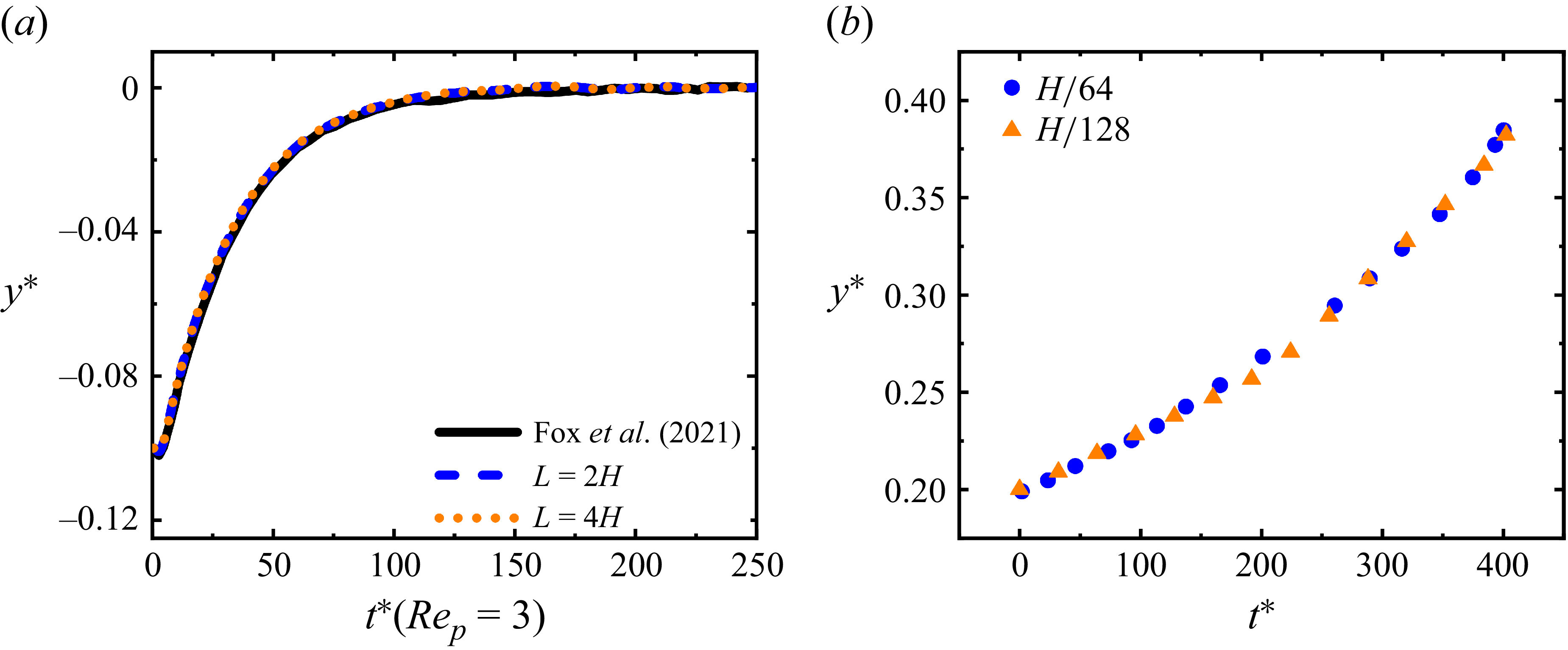
The present numerical approach has been thoroughly validated in our previous studies (Yu & Shao Reference Yu and Shao2007; Yu et al. Reference Yu, Wang, Lin and Hu2019). Yu et al. (Reference Yu, Wang, Lin and Hu2019) compared particle-migration results in two-dimensional Oldroyd-B Poiseuille flow obtained using the FD method with those computed by an arbitrary Lagrangian–Eulerian finite-element method, thus providing further validation of the FD approach. In figure 2, we further validate the present method by considering the migration of a spherical particle in Newtonian and Oldroyd-B fluids. For the Newtonian case, figure 2(a) presents the particle trajectories obtained at Re
p
= 3, β = 0.4 and y
0 = −0.1H. Unless otherwise stated, ρ
r
= 1 and η
r
= 0.5 are used in all Oldroyd-B simulations. Simulations conducted using domain lengths L = 2H and L = 4H yield nearly identical migration trajectories, indicating that the particle motion is insensitive to further extension of the computational domain. Moreover, the present results agree well with those reported by Fox et al. (Reference Fox, Schneider and Khair2021). Therefore, L = 2H is adopted in the subsequent simulations to reduce the computational cost without compromising numerical accuracy. For the viscoelastic case, owing to the limited number of relevant studies currently available, figure 2(b) compares the results obtained using the present code at different grid resolutions for Re = 0.2, β = 0.2 and Wi = 1, thereby providing further support for the accuracy of the DF/FD method. To achieve a suitable balance between computational cost and numerical accuracy, computational domain length L = 2H and grid spacing
 $\Delta$
x = H/128 are adopted, and a time step is chosen as
 $\Delta$
t = 5 × 10⁻⁴. Unless otherwise specified, all parameter settings are kept identical to those described above.
(a) Validation for the Newtonian fluid case and the computational domain size. (b) Validation for the viscoelastic fluid case and the grid-independence test.

3. Results and discussion
3.1. Migration of a spherical particle
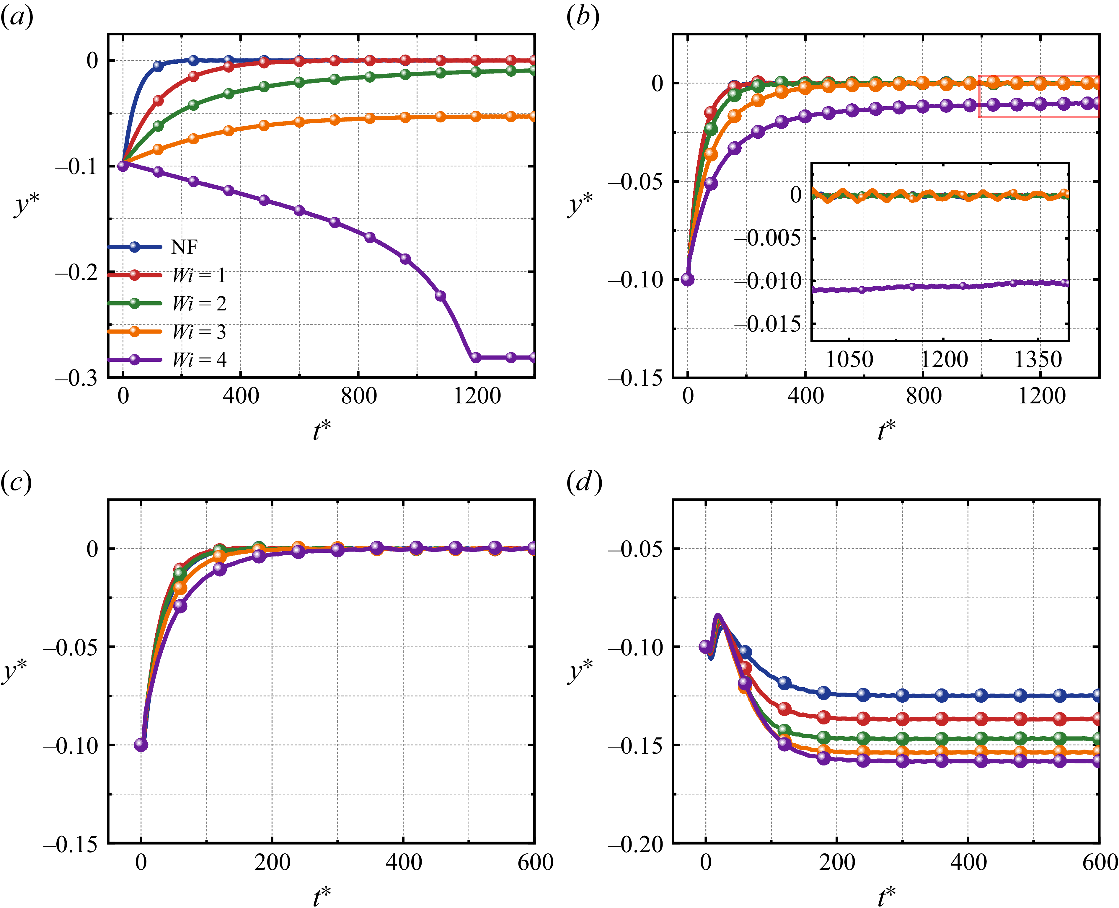
This subsection examines the lateral migration of a spherical particle suspended in an Oldroyd-B shear flow, with the blockage ratio fixed at β = 0.2. The particle position and time are non-dimensionalised by the channel height (y * = y/H) and the inverse shear rate (t * = Gt), respectively, while the lift force F L is normalised by the characteristic scale ρ f U 0 2 a 4/H 2. The particle is initially released from y * = −0.1 and allowed to translate and rotate freely until it reaches equilibrium in the y-direction. The results show that at Re p = 0.4, the equilibrium position of the particle bifurcates from the centreline towards the wall as the Weissenberg number Wi increases. As the Reynolds number increases to Re p = 1 and 3, the equilibrium position shifts back towards the centreline. At Re p = 10, however, the migration direction reverses towards the wall, and the equilibrium position moves progressively closer to the wall with increasing Wi.
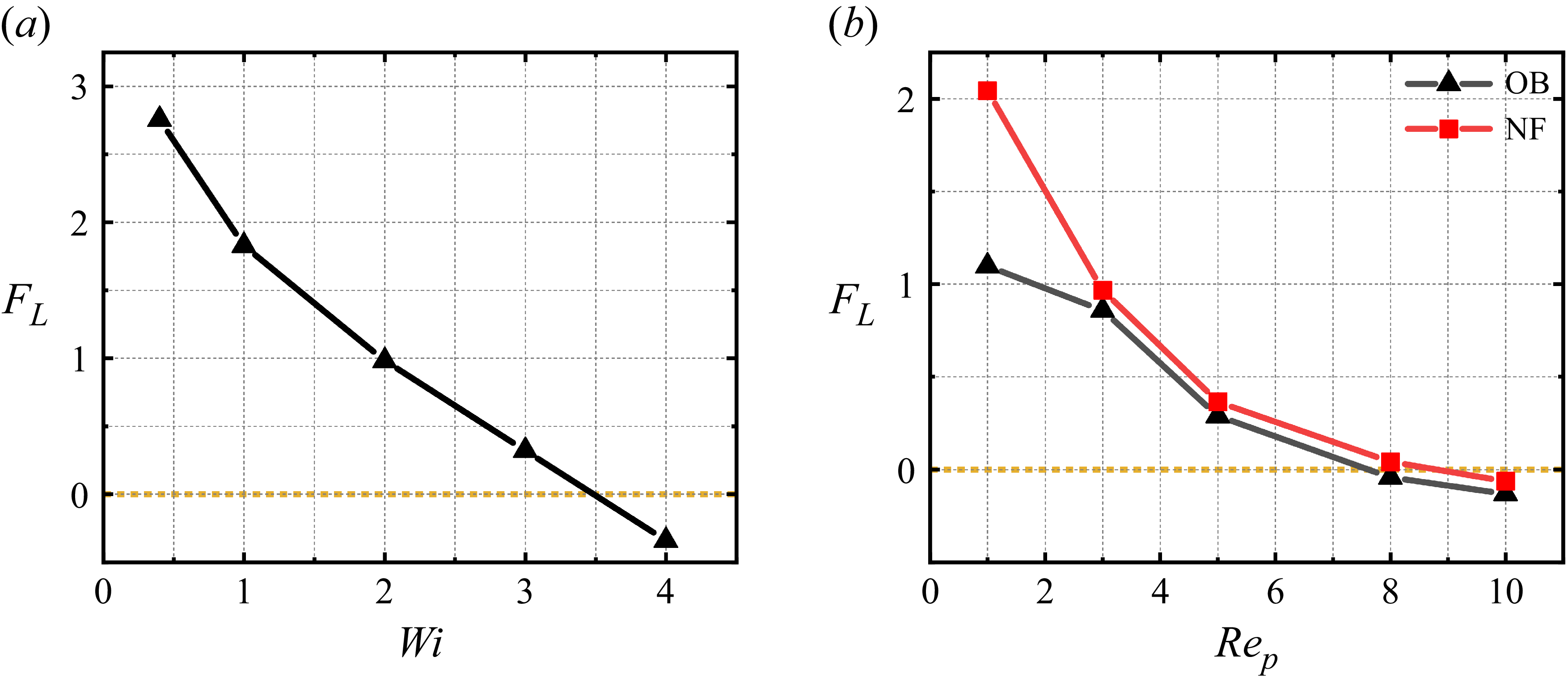
Figure 3(a) shows the migration trajectory of the particle at Re p = 0.4. The results indicate that when Wi < 4, the particle migrates towards the centreline, whereas at Wi = 4, the migration reverses and the final equilibrium position is approximately y * = −0.28. To elucidate the mechanism responsible for this behaviour, the particle was fixed at y * = −0.1 while being allowed to translate and rotate freely in the flow direction. The resulting lift force, shown in figure 4(a), is defined as positive towards the channel centreline. At Re p = 0.4, the lift force F L decreases monotonically with increasing Wi. The magnitude of F L correlates strongly with the final equilibrium position: a larger F L corresponds to an equilibrium position closer to the centreline (y *→0). Therefore, the sign of F L dictates the migration direction (towards or away from the centreline), whereas its magnitude determines the equilibrium distance. Fox et al. (Reference Fox, Schneider and Khair2021) showed that in Newtonian fluids, the particle equilibrium position depends on the F L experienced at its initial release location. Unlike the Newtonian inertial lift, the elastic contribution is not unidirectional; its direction depends on the local polymer-stress distribution around the particle.
Variation of the particle equilibrium position with dimensionless time t * at different Re p : (a) Re p = 0.4, (b) Re p = 1, (c) Re p = 3, (d) Re p = 10. Here, NF stands for Newtonian fluid.

Figure 3. Long description
Panel A: A line graph shows the variation of particle equilibrium position y* over dimensionless time t* for Rep = 0.4. The x-axis represents dimensionless time t* ranging from 0 to 1200, and the y-axis represents the particle equilibrium position y* ranging from -0.3 to 0. The graph includes five lines representing different Wi values (NF, Wi = 1, Wi = 2, Wi = 3, Wi = 4) with distinct colors. Panel B: A line graph shows the variation of particle equilibrium position y* over dimensionless time t* for Rep = 1. The x-axis represents dimensionless time t* ranging from 0 to 1350, and the y-axis represents the particle equilibrium position y* ranging from -0.15 to 0. The graph includes five lines representing different Wi values (NF, Wi = 1, Wi = 2, Wi = 3, Wi = 4) with distinct colors. An inset zooms in on the time range from 1050 to 1350. Panel C: A line graph shows the variation of particle equilibrium position y* over dimensionless time t* for Rep = 3. The x-axis represents dimensionless time t* ranging from 0 to 600, and the y-axis represents the particle equilibrium position y* ranging from -0.15 to 0. The graph includes five lines representing different Wi values (NF, Wi = 1, Wi = 2, Wi = 3, Wi = 4) with distinct colors. Panel D: A line graph shows the variation of particle equilibrium position y* over dimensionless time t* for Rep = 10. The x-axis represents dimensionless time t* ranging from 0 to 600, and the y-axis represents the particle equilibrium position y* ranging from -0.2 to -0.05. The graph includes five lines representing different Wi values (NF, Wi = 1, Wi = 2, Wi = 3, Wi = 4) with distinct colors.
Dimensionless F L acting on the particle at a fixed position y * = −0.1. (a) Relationship between F L and Wi at Re p = 0.4. (b) Comparison of F L andRe p between viscoelastic Oldroyd-B (OB) fluid (Wi = 4) and Newtonian fluid (NF).

At Re p = 10 (figure 3 d), the particle initially migrates toward the channel centreline, but its migration reverses at y * = −0.07, ultimately reaching an equilibrium position below its release position (closer to the wall). Compared with Newtonian fluids, the equilibrium position in the viscoelastic fluid shifts progressively towards the wall as Wi increases. The corresponding lift force F L (figure 4 b) is negative, indicating a force directed away from the centreline (towards the wall), which is consistent with the observed migration direction.
At 1 ≤ Re p ≤ 3 (figures 3 b,c), the particle equilibrium returns to and remains near the channel centreline. For Re p = 1, the particle equilibrium in the viscoelastic fluid coincides with that in the Newtonian case for Wi ≤ 3. A slight lateral deviation towards the wall is observed only when Wi = 4 (figure 3 b). For Re p = 3, the particle equilibrium positions for all examined Wi values match those in the Newtonian fluid. Figure 4(b) compares the lift force F L in Oldroyd-B and Newtonian fluids as a function of Re p for Wi = 4. The results show that F L in the viscoelastic fluid decreases monotonically with increasing Re p , consistent with the trends reported by Fox et al. (Reference Fox, Schneider and Khair2021). Moreover, the lift distribution across the channel exhibits a monotonic spatial variation. Notably, at Re p = 1 and Wi = 4, a small offset of the equilibrium position from the centreline is observed; this offset vanishes at Re p = 3, where the equilibrium returns to the centreline. Although a larger F L would be expected to draw the particle closer to the centreline, a special case occurs at Re p = 1 and Wi = 4. Further analysis indicates that this apparent contradiction arises from an asymmetric distribution of the first normal-stress difference N 1 above and below the particle. The additional elastic forcing associated with this N 1 asymmetry can counteract or modify the simple F L -based prediction, thereby producing the observed offset in the equilibrium position.
To further elucidate the mechanisms responsible for particle migration towards the shear-layer centre or the wall in a viscoelastic shear flow, we analyse the surface-resolved contributions of the hydrodynamic forces acting on the particle. A non-body-fitted finite-difference framework is employed, in which the flow field and stresses in the vicinity of the particle boundary are reconstructed via interpolation. The resulting surface stresses are then integrated to obtain the net force. The transverse lift force acting on the particle in the y-direction, F L , is decomposed into three primary components: the pressure contribution F p , the viscous contribution F V , and the polymeric (elastic) contribution F E . The corresponding expressions are
 \begin{align} F_{\kern-1pt p}=\int _{\partial \kern-1pt P}-n_{y}p \mathrm{d}S, \\[-28pt] \nonumber \end{align}
 \begin{align} F_{V}=\eta _{s}\int _{\partial \kern-1pt P}\left[2n_{y}\frac{\partial u_{y}}{\partial y}+n_{x}\left(\frac{\partial u_{y}}{\partial x}+\frac{\partial u_{x}}{\partial y}\right)+n_{z}\left(\frac{\partial u_{y}}{\partial z}+\frac{\partial u_{z}}{\partial y}\right)\right]\mathrm{d}S, \\[-28pt] \nonumber \end{align}
 \begin{align} F_{\kern-1pt E}=\int _{\partial \kern-1pt P}\left(n_{x}\tau _{xy}+n_{y}\tau _{yy}+n_{z}\tau _{yz}\right) \mathrm{d}S. \\[-12pt] \nonumber \end{align}
The polymer force (F E ) can be further decomposed into the polymer normal force (F En ) and the polymer shear force (F Es ):
 \begin{align} F_{\kern-1pt En}=\int _{\partial \kern-1pt P}n_{y}\tau _{yy} \mathrm{d}S, \\[-28pt] \nonumber \end{align}
 \begin{align} F_{Es}=\int _{\partial \kern-1pt P}\left(n_{x}\tau _{xy}+n_{z}\tau _{yz}\right) \mathrm{d}S. \\[0pt] \nonumber \end{align}
The pressure force in (3.1) is calculated from the pressure to satisfy the incompressibility constraint. In a viscoelastic fluid, the polymer isotropic stress (τ xx + τ yy + τ zz )/3 or the average polymer normal stresses can also be regarded as ‘pressure’, and the elasticity induced force is related to the normal-stress differences (Ho & Leal Reference Ho and Leal1976). Therefore, the polymer normal force F En can be decomposed into the polymer ‘pressure’ force F Enp , the force from the first normal-stress difference F En1, and the second normal-stress difference F En2:
 \begin{align} F_{\kern-1pt En}=\underset{F_{Enp}}{\underbrace{\int _{\partial \kern-1pt P}n_{y}\frac{\tau _{xx}+\tau _{yy}+\tau _{zz}}{3}\,\mathrm{d}S}}+\underset{F_{En1}}{\underbrace{\int _{\partial \kern-1pt P}n_{y}\frac{\tau _{yy}-\tau _{zz}}{3}\,\mathrm{d}S}}+\underset{F_{En2}}{\underbrace{\int _{\partial \kern-1pt P}n_{y}\frac{\tau _{yy}-\tau _{xx}}{3}\,\mathrm{d}S}}.{\quad} \end{align}
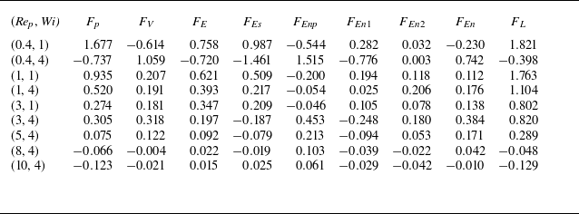
Combining figures 3(a–d) with table 1 shows that Re p governs the transition from an elasticity-sensitive regime to an inertia-dominated one, whereas Wi primarily amplifies polymer contributions at low Re p , and can even reverse the migration direction. At Re p = 0.4, increasing Wi from 1 to 4 changes the net lateral force from positive to negative (F L 1.821 → −0.398), thereby switching the trajectory from centreline-directed to wall-directed migration. This reversal is mainly caused by a strong, sign-changing polymer shear traction (F Es 0.987 → −1.461), which, together with the pressure component, drives the motion while the viscous contribution provides an opposing (compensating) effect. As Re p increases to 1–3, the net force remains centreline-directed (F L 1.104–1.763 at Re p = 1, and F L 0.802–0.820 at Re p = 3), and Wi mainly modulates the magnitude and internal partitioning without changing the sign: at Re p = 1, F p remains the largest contribution (0.935 → 0.520), whereas at Re p = 3, the dominant balance shifts from polymer-dominated at Wi = 1 (F E = 0.347 being the largest term) to a pressure–viscous comparable balance at Wi = 4 (F V = 0.318 ≈ F p = 0.305). At Re p = 10, the dynamics becomes essentially pressure (inertial) controlled (Wi = 4, F p = −0.123 ≈ F L = −0.129), and Wi only introduces minor corrections; consequently, the trajectories are dictated by high-Re p inertial lift, and exhibit a pronounced off-centre equilibrium.
Forces on a particle at fixed y-position as functions of Re p and Wi.

Table 1. Long description
A table with 8 rows and 12 columns. The columns are labeled as Rep, Wi, Fp, Fv, FE, FEs, FEnp, FEn1, FEn2, FEn, and FL. The table presents numerical values for different combinations of Rep and Wi. Row 1: Rep, Wi, Fp, Fv, FE, FEs, FEnp, FEn1, FEn2, FEn, FL; 0.4, 1, 1.677, -0.614, 0.758, 0.987, -0.544, 0.282, 0.032, -0.230, 1.821. Row 2: 0.4, 4, -0.737, 1.059, -0.720, -1.461, 1.515, -0.776, 0.003, 0.742, -0.398. Row 3: 1, 1, 0.935, 0.207, 0.621, 0.509, -0.200, 0.194, 0.118, 0.112, 1.763. Row 4: 1, 4, 0.520, 0.191, 0.393, 0.217, -0.054, 0.025, 0.206, 0.176, 1.104. Row 5: 3, 1, 0.274, 0.181, 0.347, 0.209, -0.046, 0.105, 0.078, 0.138, 0.802. Row 6: 3, 4, 0.305, 0.318, 0.197, -0.187, 0.453, -0.248, 0.180, 0.384, 0.820. Row 7: 5, 4, 0.075, 0.122, 0.092, -0.079, 0.213, -0.094, 0.053, 0.171, 0.289. Row 8: 8, 4, -0.066, -0.004, 0.022, -0.019, 0.103, -0.039, -0.022, 0.042, -0.048. Row 9: 10, 4, -0.123, -0.021, 0.015, 0.025, 0.061, -0.029, -0.042, -0.010, -0.129.
To clarify the intriguing behaviour described above, we further examine the deformation characteristics of the polymer molecules in the viscoelastic fluid. Specifically, we analyse the distribution of polymer stretch (extension) in the vicinity of the particle at equilibrium for Re
p
= 1 and Re
p
= 3. The first normal-stress difference is defined as
N
1 =
 $ \boldsymbol{\tau} $
zz
−
 $ \boldsymbol{\tau} $
yy
, where
 $ \boldsymbol{\tau} $
zz
and
 $ \boldsymbol{\tau} $
yy
are the streamwise and transverse normal stresses, respectively. In addition, the trace of the conformation tensor, tr(
C
), quantifies the average polymer extension, reflecting the overall conformational deformation of polymers under complex flow. Since the velocity gradient at the particle–fluid interface is subject to oscillations induced by the discrete δ-functions, the conformation tensor evaluated from it inevitably incorporates pseudo-diffusive effects. Therefore, the present analysis is used only for qualitative interpretation. The detailed analysis is presented as
 \begin{align} \boldsymbol{C}=\frac{\lambda _{t}}{\eta _{p}}\boldsymbol{\tau }\boldsymbol{+}\boldsymbol{I} . \end{align}
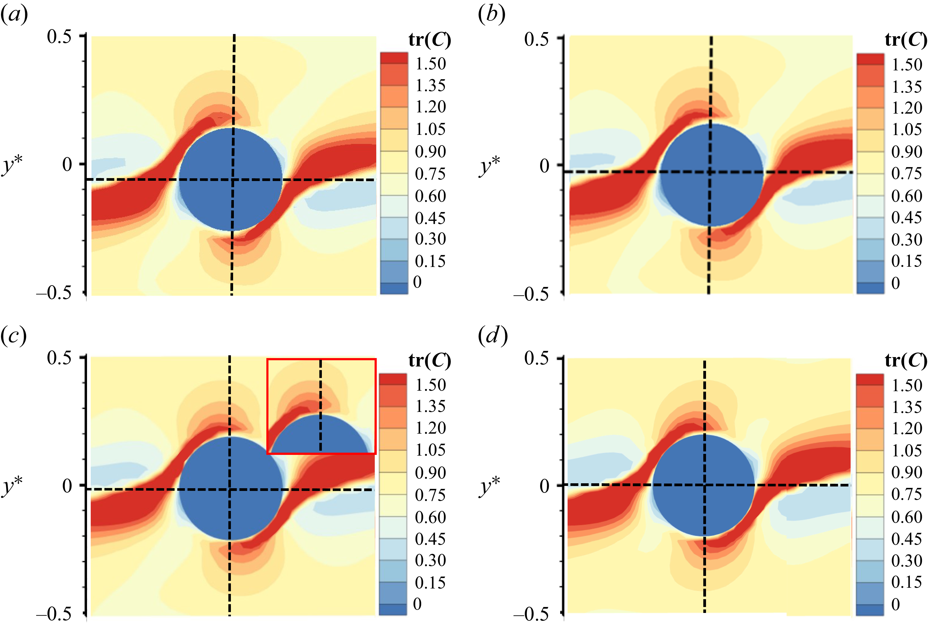
Figure 5(c) shows the polymer-extension (conformation) field around the particle at Re p = 1 and Wi = 4. A region of strongly stretched polymers develops along the flow direction and extends upwards from the particle. The magnified view in figure 5(c) shows that unlike the polymer stretching observed above the particle, the stretching region below the particle does not extend across its mid-plane. From this magnified view, the polymer-extension distribution is clearly asymmetric between the region above the particle ( U p ) and that below it ( D p ). The asymmetric stretching of this polymer has already occurred during the migration process. As shown in figure 5(a), at t * = 100, the polymer deformation beneath the particle is stronger than that above it, which coincides with the onset of the particle’s migration towards the channel centreline. In figure 5(b), by t * = 200, the polymer deformation around the particle evolves into the opposite pattern, with stronger deformation above the particle than below. This distribution is consistent with that observed when the particle eventually settles at its off-centre equilibrium position. By contrast, figure 5(d) shows that at equilibrium for Re p = 3 and Wi = 4, the polymer extension field becomes more symmetric.
(a,b) The polymer deformation around the particle at the initial stage of motion for Re p = 1 and Wi = 4: (a) t ∗ = 100, (b) t ∗ = 200. (c,d) The deformation after the particle reaches its equilibrium position: (c) Re p = 1, Wi = 4; (d) Re p = 3, Wi = 4.

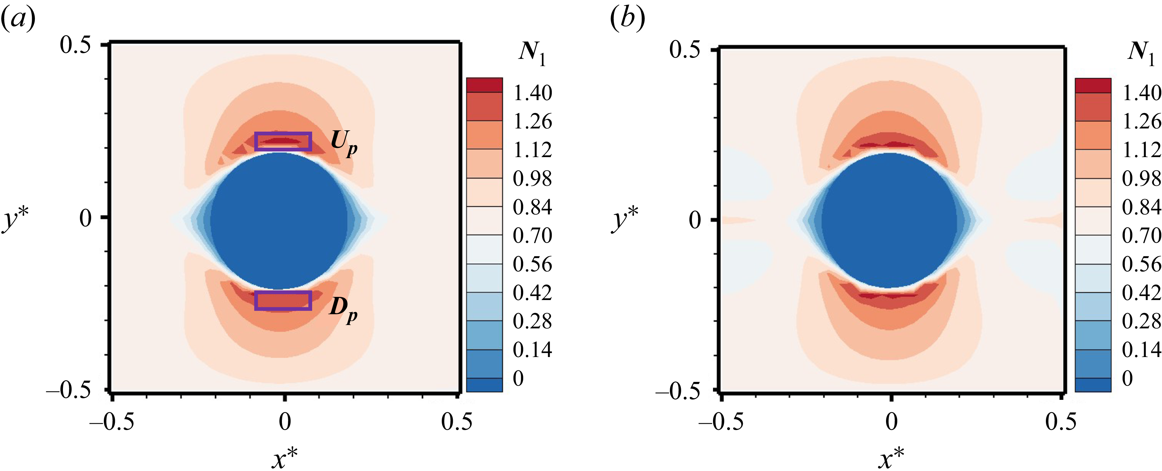
This asymmetry is directly reflected in the distribution of N 1, as shown in figure 6(a): the N 1 values in the U p and D p regions differ markedly. At Re p = 3 and Wi = 4, however, the corresponding asymmetry in both polymer extension and N 1 is greatly diminished, yielding an approximately symmetric configuration. Hu et al. (Reference Hu, Lin, Zhu, Yu, Lin and Li2024) reported that particles tend to migrate from regions of high N 1 to regions of lower N 1, i.e. towards areas of reduced local normal-stress difference. Here, U p and D p denote the regions above and below the particle, respectively (as shown in figure 6 a), and |△N 1 | is defined as the absolute difference between the N 1 values in the two regions.
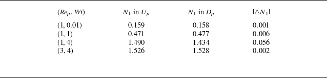
Table 2 reports the spatial average of N 1, evaluated along the vertical direction on the particle-centred cross-section (x = 0) after the particle has reached its equilibrium position, to quantify the influence of polymer deformation on the local stress field. The results show that increasing the Weissenberg number Wi leads to a pronounced increase of N 1 in both the U p and D p regions, with N 1 reaching its maximum at Re p = 3 and Wi = 4. In viscoelastic fluids, the lateral elastic force on a particle generally points towards regions of lower N 1. Accordingly, the asymmetry in the spatial gradient of the N 1 distribution is the primary factor determining the direction of particle migration (Li et al. Reference Li, McKinley and Ardekani2015; Naderi et al. Reference Naderi, Barilla, Zhou, Papautsky and Peng2022).
Mean values of N 1 in the U p and D p regions.

Table 2. Long description
The table presents mean values of N1 in the Up and Dp regions for different (Rep, Wi) pairs. It has four rows and three columns. The columns are labeled as (Rep, Wi), N1 in Up, N1 in Dp, and |N1|. The rows are as follows: Row 1: (1, 0.01), 0.159, 0.158, 0.001. Row 2: (1, 1), 0.471, 0.477, 0.006. Row 3: (1, 4), 1.490, 1.434, 0.056. Row 4: (3, 4), 1.526, 1.528, 0.002.
Distribution of N 1 around the particle on the x–y plane when the particle attains its equilibrium position: (a) Re p = 1, Wi = 4; (b) Re p = 3, Wi = 4.

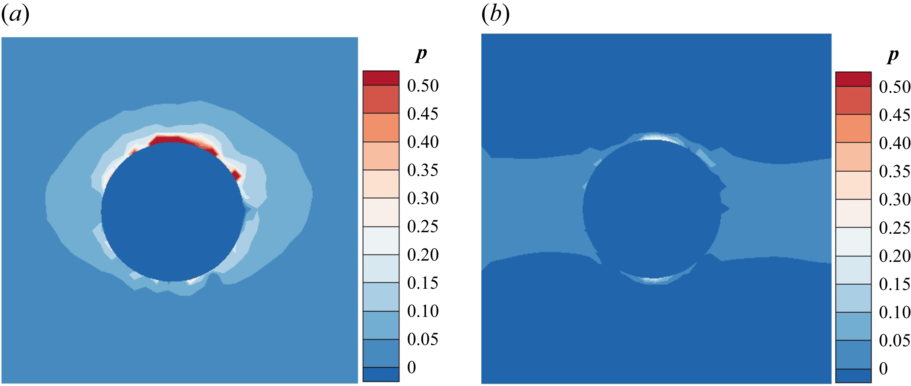
The absolute difference of N 1 between the upper and lower regions of the particle, denoted as |Δ N 1|, is summarised in table 2. At Re p = 1, |Δ N 1| increases with Wi and attains its maximum at Wi = 4, indicating that the asymmetry in the normal-stress field is most pronounced under these conditions. This asymmetry induces a local high-pressure zone above the particle (figure 7 a). The resulting pressure imbalance causes the particle – which would otherwise migrate towards the centreline – to deviate from its expected trajectory. In contrast, at Re p = 3 and Wi = 4, although the overall magnitude of N 1 in the upper and lower regions remains high, the difference |Δ N 1| is small. As shown in figure 7(b), the pressure distribution becomes nearly symmetric, producing a balanced normal-stress field that confines the particle near the channel centreline.
Pressure field on the x–y plane when the particle attains its equilibrium position: (a) Re p = 1, Wi = 4; (b) Re p = 3, Wi = 4.

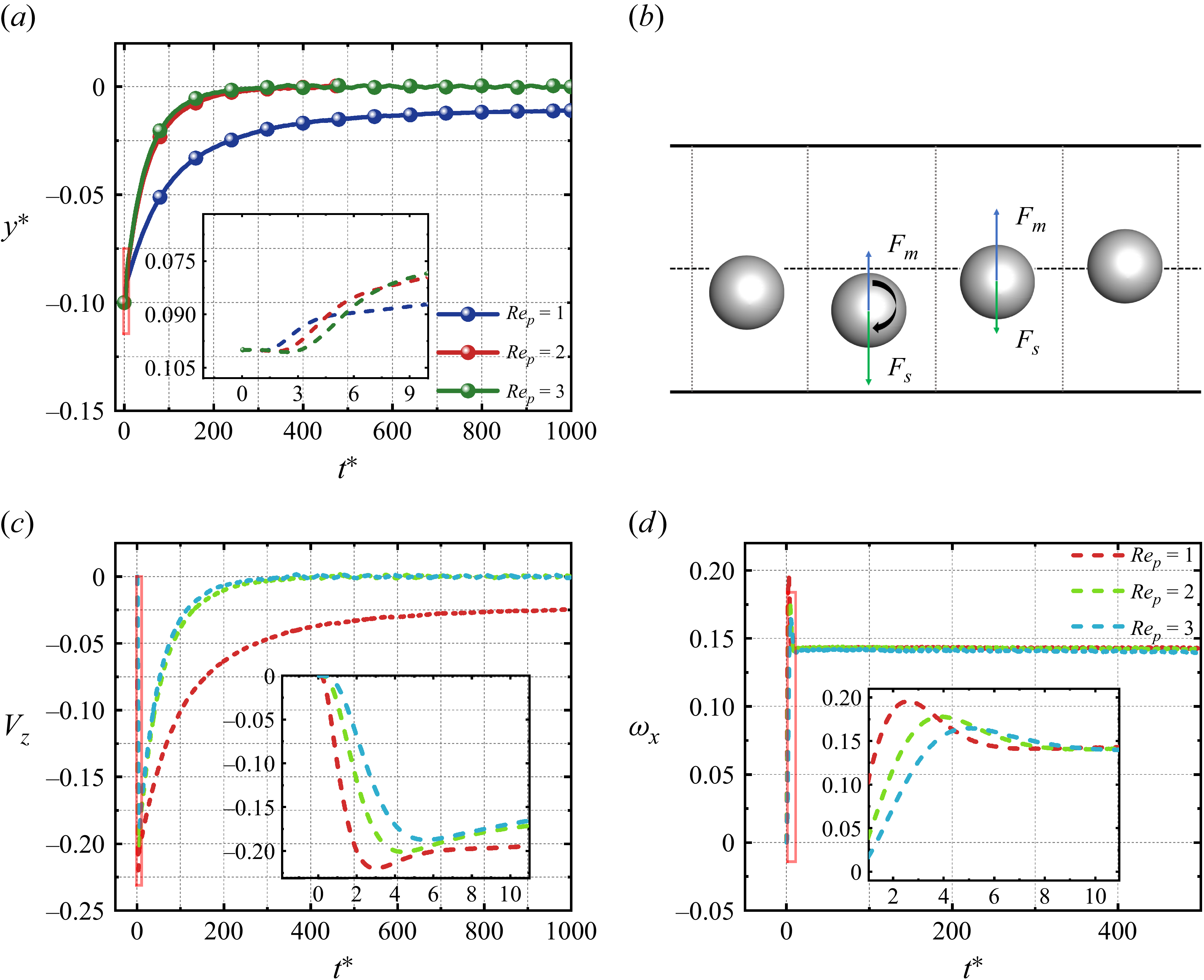
The lateral migration of a particle is an intrinsically time-dependent process. In viscoelastic fluids, the lateral lift force F L acting on the particle decreases with increasing Re p . Figure 8(a) presents the particle migration trajectories for different Re p at Wi = 4. On the same time scale, the trajectories for Re p = 2 and Re p = 3 lie above that for Re p = 1; i.e. particles experiencing smaller instantaneous lift show larger lateral displacement during this stage. Superficially, this observation appears inconsistent with a simplified, instantaneous-force expectation (a naive reading of Newton’s second law). A closer view of the inset in figure 8(a) reveals that the particles initially drift slightly towards the wall before returning towards the centreline. Motivated by this observation, the migration process may be divided into three distinct stages (figure 8 b): an approach-to-wall (descent) stage, a return-to-centre (rebound) stage, and a final equilibrium stage. For simplified comparison at fixed Wi, we temporarily neglect time-dependent elastic contributions, and approximate the lateral lift as the sum of two components: (i) the Saffman lift F s induced by velocity gradients and dependent on the relative velocity V 0 between the particle and the surrounding fluid; (ii) the Magnus lift F m arising from particle rotation. The resultant of these two lift components governs the instantaneous lateral motion. It should be noted that the measured F L in this study corresponds to an estimate of the combined lift components when the particle is in a quasi-steady state near its initial position.
Migration of a spherical particle in a viscoelastic shear flow: (a) particle trajectory, (b) initial migration state, (c) lateral migration velocity, (d) angular velocity about the x 0-axis.

Saffman (Reference Saffman1965) calculated a lift force scaling as |F s |∼ 6.46aη 0|V 0|Re p 1/2, where |V 0| represents the relative velocity. Figures 8(c) and 8(d) show the temporal evolution of the particle’s translational and angular velocities during the initial stage of migration. Following wall start-up, the surrounding fluid accelerates more rapidly than the particle, generating a transient slip velocity V 0 = V f – V z . This relative motion generates a downward Saffman lift F s , driving the particle towards the lower channel wall. As the particle’s angular velocity about the x 0-axis, ω x , increases, the Magnus lift F m strengthens; once F m > F s , the particle reverses direction and migrates upwards. A close inspection of figure 8(c) shows that the post-peak decay rate of the particle velocity is significantly larger for Re p = 2, 3 than for Re p = 1. This indicates that the particle–fluid relative velocity V 0 is smaller at higher Re p , and consequently F s is weaker. Because the three Re p cases exhibit approximately the same angular velocity ω x during the rebound stage, the corresponding F m is approximately comparable across cases. It follows that the net lift F L during the rebound stage is likely smaller for Re p = 1 than for Re p = 2, 3. This behaviour contradicts the trend observed at the initial stage that the lift increases as Re p decreases. This indicates that the initial lift, while setting the migration direction, is insufficient to account for the full dynamical evolution. At later times, the particle settles into one of two distinct equilibrium states: a centred stable state (Re p = 2, 3) or an eccentric stable state (Re p = 1). In the centred state, the particle remains near the channel centreline, where the upstream and downstream flows are approximately symmetric and forces balance. In the eccentric state, the particle equilibrates off-centre while maintaining a finite streamwise velocity and rotation; the persistent particle–fluid relative motion produces a downward F s that is balanced by the spin-induced F m . Previous results indicate that at Re p = 0.4, multiple equilibrium positions may arise as Wi increases. A similar bifurcation appears near Wi = 4 for Re p = 1, whereas no such bifurcation occurs for Re p = 2, 3. This observation suggests that in viscoelastic fluids, the equilibrium position becomes less stable when Re p < 1.
3.2. Migration of an oblate particle
Compared with geometrically symmetric spheres, non-spherical particles possess additional orientational degrees of freedom arising from shape anisotropy, which leads to substantially more complex dynamics in viscoelastic fluids. For spherical particles, lateral migration reflects a competition between inertial and elastic lift forces. When the particle shape departs from sphericity and becomes an oblate spheroid, this force balance not only determines lateral focusing positions, but also substantially alters the rotational modes and their stability. A systematic investigation across Re p and Wi is therefore required to elucidate how shape anisotropy governs particle migration and orientational dynamics.
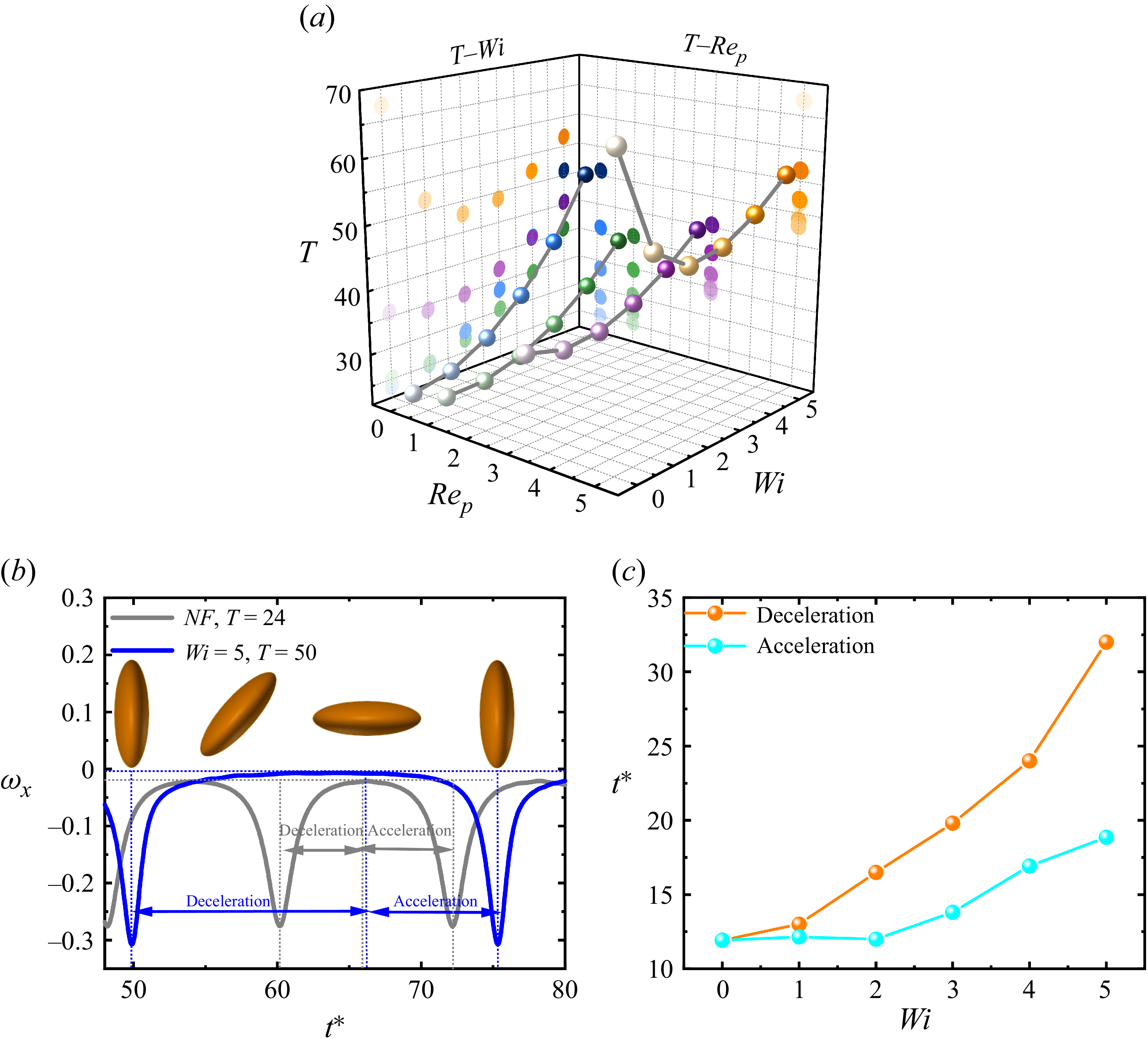
The initial position and orientation of the oblate particle are y * = −0.1 and n p1, respectively. Due to geometric anisotropy, an oblate particle in shear flow can rotate about its major axis; we refer to this rotation mode as the ‘tumbling’ state. The initial sense of rotation is aligned with the shear direction, as shown in figure 1(a). As the flow evolves towards steady state, the particle transitions to a periodic in-plane rotation, referred to as the rolling state. Finite inertia and wall confinement can modify the classical Jeffery dynamics and promote the selection of stable rotational states. Figure 9(a) shows the particle rotation period T, defined as the time required for the particle to complete one full revolution for different values of Wi and Re p . For Re p ≤ 3, the rotation period in the viscoelastic fluid is generally larger than that in the corresponding Newtonian case. Li et al. (Reference Li, Xu and Zhao2023) reported a similar trend for prolate ellipsoids, showing that increasing fluid elasticity significantly prolongs the rotation period. Figure 9(b) displays a representative single-period rotation at Re p = 0.1.
(a) Rotation period of an oblate spheroidal particle as a function of Wi. (b) Particle motion regime and its acceleration/deceleration phases. (c) Duration of acceleration and deceleration phases as a function of Wi at Re p = 0.1.

Figure 9. Long description
Panel A: A 3D scatter plot shows the rotation period (T) of an oblate spheroidal particle as a function of Wi (Weissenberg number) and Re_p (particle Reynolds number). The axes are labeled with T, Wi, and Re_p. The plot includes multiple data points in various colors, indicating different conditions or measurements. Panel B: A line graph depicts the particle motion regime and its acceleration and deceleration phases. The horizontal axis is labeled t* (dimensionless time), and the vertical axis is labeled ω_x (angular velocity). Two lines are shown: one for Newtonian fluid (NF) with T = 24 and another for Wi = 5 with T = 50. The graph includes annotations for deceleration and acceleration phases. Panel C: A line graph shows the duration of acceleration and deceleration phases as a function of Wi at Re_p = 0.1. The horizontal axis is labeled Wi, and the vertical axis is labeled t* (dimensionless time). Two lines are shown: one for deceleration and another for acceleration, with data points marked in different colors.
Increasing Wi breaks the temporal symmetry between the acceleration and deceleration phases that is present in Newtonian shear flow. Jeffery (Reference Jeffery1922) derived the orientation dynamics of ellipsoids in simple shear, yielding an analytical angular-velocity evolution with strict angular periodic symmetry. This Jeffery symmetry is, however, broken in viscoelastic fluids. Figure 9(c) compares the durations of the acceleration and deceleration phases within a single Jeffery orbit: the deceleration phase is substantially longer than the acceleration phase, and the disparity increases monotonically with Wi. This indicates that fluid elasticity increases the rotation period primarily by prolonging the deceleration phase. It is noteworthy that in Newtonian fluids, the rotation period increases with Re p ; at Re p = 5, the period even exceeds that observed in viscoelastic fluids under comparable conditions (Wi > 0).
To systematically assess the effect of the Weissenberg number Wi on the Jeffery-orbit period of an oblate particle, figure 10 shows the polymer conformation/deformation field at Re p = 0.1. Figures 10(a–d) and 10(e–h) correspond to Wi = 1 and Wi = 5, respectively; the particle rotates in the direction indicated by the arrows. In figure 10(a), the polymer extension is initially concentrated near the particle long axis, indicating that polymers near the tip are the first to experience significant stretching. When the particle z 0-axis becomes aligned with the flow z-axis (figure 10 b), the polymer extension reaches its maximum, coinciding with the peak in particle rotation speed (figure 9 b). Following this peak, the highly stretched polymer region is convected past the particle tip, and moves to the opposite side (figure 10 c). As the particle’s z 0-axis tilts from alignment with the flow direction towards the migration, the over-stretched polymer chains begin to relax. This relaxation releases stored elastic stresses, generating a reverse torque that slows the particle’s rotation. Because viscoelastic fluids relax stresses on a characteristic time scale λ t , the elastic stress response to deformation shows a pronounced lag (Ewoldt & Saengow Reference Ewoldt and Saengow2022). This lag causes the release of elastic stresses only after the polymers have reached their maximum extension, thereby lengthening the time required for the particle’s angular velocity to decay to zero. The resulting delayed relaxation produces a strong temporal asymmetry in the Jeffery orbit – specifically, unequal acceleration and deceleration durations. When the particle returns to its initial orientation (figure 10 d), half the rotation period is completed, and the surrounding polymer conformation gradually relaxes back towards its initial state. At Wi = 5 (figures 10 e–h), polymer stretching is substantially larger; consequently, the lagged elastic stress response is stronger, further prolonging the deceleration stage and increasing the overall rotation period.
Distribution of the trace of the conformation tensor on the x = 0 plane around the particle at Re p = 0.1: (a–d) Wi = 1, (e–h) Wi = 5.

Final steady-state motion modes of the particle: (a) tumbling, (b) rolling, (c) kayaking, (d) translation, (e) stable particle orientation for parameter n p1, (f) stable particle orientation for parameter n p2.

Figure 11. Long description
Panel A: A 3D diagram shows a particle tumbling in shear flow. The right graph is a line graph depicting angular velocity (ω) over time (t*). The axes are labeled with ω_x, ω_y, and ω_z representing different components of angular velocity. Panel B: A 3D diagram shows a particle rolling in shear flow. The right graph is a line graph depicting angular velocity (ω) over time (t*). The axes are labeled with ω_x, ω_y, and ω_z representing different components of angular velocity. Panel C: A 3D diagram shows a particle kayaking in shear flow. The right graph is a line graph depicting angular velocity (ω) over time (t*). The axes are labeled with ω_x, ω_y, and ω_z representing different components of angular velocity. Panel D: A 3D diagram shows a particle translating in shear flow. The right graph is a line graph depicting angular velocity (ω) over time (t*). The axes are labeled with ω_x, ω_y, and ω_z representing different components of angular velocity. Panel E: A scatter plot shows the relationship between the dimensionless particle Reynolds number (Re_p) and the dimensionless Wi. Different symbols represent different motion modes: Translation(a), Rolling, Tumbling, Kayaking, and Translation(b). Panel F: A scatter plot shows the relationship between the dimensionless particle Reynolds number (Re_p) and the dimensionless Wi. Different symbols represent different motion modes: Kayaking, Inclined rolling, Rolling, and Translation(b).
(a) Particle trajectory at Re p = 0.1. (b) Evolution of the lift force F L with dimensionless time (t *) for different values of Wi. (c) Evolution of the angular velocity with dimensionless time (t *) for different values of Wi. (d) First normal-stress difference N 1 for a particle in translation near the wall.

Figure 12. Long description
Panel A: A line graph shows the particle trajectory over dimensionless time (t*) for different Weissenberg numbers (Wi). The y-axis represents the cross-stream position (y*) and the x-axis represents dimensionless time (t*). Different lines represent different Wi values, showing how particle trajectory changes with varying Wi. Panel B: A line graph depicts the evolution of the lift coefficient (FL) with dimensionless time (t*) for different Wi values. The y-axis represents the lift coefficient (FL) and the x-axis represents dimensionless time (t*). Different lines represent different Wi values, illustrating how the lift coefficient evolves over time for each Wi. Panel C: Three line graphs show the evolution of the angular velocity (ω) with dimensionless time (t*) for different Wi values. The y-axis represents the angular velocity (ω) and the x-axis represents dimensionless time (t*). Each graph corresponds to a different Wi value, showing how angular velocity changes over time for each Wi. Panel D: A color map visualizes the first normal-stress difference (N1) for a particle in translation near the wall. The color scale indicates the magnitude of N1, with red representing higher values and blue representing lower values.
The tumbling state typically appears during the early stage after an oblate particle with initial orientation n p1 enters the shear flow. As the particle migrates towards its equilibrium position, its final rotational mode is governed by the competing influences of three contributions: fluid inertia, particle inertia, and elastic forces arising from the viscoelastic medium. Figures 11(a–d) present schematic examples of four characteristic motion modes: (a) tumbling, (b) rolling, (c) kayaking and (d) translation. Rolling can be further categorised into log-rolling and inclined rolling, while translation may be classified as near-wall sliding or angled translation. The results indicate that rolling remains the dominant equilibrium mode over most of the parameter space explored. However, consistent with previous studies, the dynamics of non-spherical particles is sensitive to the initial orientation. In the present study, we have focused on two representative orientations; if the particle is initialised at an intermediate orientation between the flow direction ( n p1) and the vorticity direction ( n p2), then both the transient trajectory and the final equilibrium orientation may change. The present results suggest that such changes are generally confined to the rotational modes near the regime boundaries in the parameter space considered.
Evolution of the oblate spheroid’s equilibrium lateral position and angular velocity with dimensionless time (t *). (a–d) Equilibrium position versus t *: (a) Re p = 1, n p1; (b) Re p = 1, n p2; (c) Re p = 3, n p1; (d) Re p = 3, n p2. (e,f) Angular velocity versus t *: (e) Re p = 1, n p1; (f) Re p = 3, n p1.

In the viscosity-dominated regime (Re p = 0.1), variations in Wi restructure the normal-stress distribution and modulate the elastic response, producing pronounced asymmetric stresses on the oblate particle surface that significantly affect particle dynamics. As shown in figure 12(a), the particle equilibrium position undergoes a bifurcation as Wi increases. In the Newtonian baseline, the particle focuses at the channel centreline. Introducing elasticity shifts the equilibrium downwards to approximately y ∗ = −0.016 at Wi = 1. Under stronger elasticity (Wi ≥ 2), the restructured normal-stress distribution drives the particle towards the wall, and the migration rate increases monotonically with Wi. To isolate the lift mechanism, figure 12(b) shows results in which the particle is held fixed at its initial position, thereby suppressing wall-normal motion while the instantaneous lift force F L is recorded. Owing to geometric anisotropy, the lift exhibits non-steady oscillations. The time-averaged lift evaluated between the two successive peaks indicates a sustained net downward force, which drives the near-wall adhesion (‘wall-sticking’). Figure 12(c) shows the particle rotational response, showing the time series of angular velocity under the same conditions. Combining with figure 11(e), these results indicate that the particle exhibits sustained tumbling in the Newtonian fluid. Introducing elasticity at Wi = 1 disrupts this motion and induces a transition to kayaking. For larger Wi (Wi > 1), the particle undergoes kayaking as it approaches the wall and eventually transitions to a translational mode due to boundary confinement. Figure 12(d) reveals a pronounced asymmetry in N 1 between the regions above and below the particle. The N 1 asymmetry generates a residual elastic torque that sustains a rotational tendency. However, the geometric confinement near the wall suppresses this rotation, and the particle ultimately attains a stable near-wall translational state.
At Re p = 1, the inertial lift for both initial orientations directs the particle towards the channel centre, and the equilibrium position returns to the channel centreline (figures 13 a,b). Under these conditions, a lateral deviation from the centre appears only when Wi ≥ 4, and the magnitude of the offset increases with fluid elasticity. As shown in figures 11(e,f), particles located near the centre predominantly exhibit rolling in steady state, whereas particles equilibrating off-centre predominantly exhibit kayaking; thus there is a strong correlation between the steady rotational mode and the lateral equilibrium position. At Re p = 3, the lateral offset increases monotonically with Wi, such that particles progressively migrate towards the wall (figures 13 c,d); despite the displacement, the steady state remains dominated by rolling. With increasing Re p , the particle rotation more readily settles into the rolling mode. Figures 13(e) and 13(f) show the time evolution of the angular velocity for Re p = 1 and Re p = 3, respectively. The results show that increasing Wi prolongs the duration of the kayaking regime, indicating that fluid elasticity significantly delays the transition from transient kayaking to steady rolling.
Equilibrium position of an oblate spheroid at higher Re p . Evolution of the equilibrium lateral position with dimensionless time t *: (a) Re p = 5, n p1; (b) Re p = 5, n p2; (c) Re p = 7, n p1; (d) Re p = 7, n p2.

Figure 14. Long description
Panel A: A line graph shows the equilibrium lateral position of an oblate spheroid at Rep = 5, np1 over dimensionless time t*. The y-axis represents the dimensionless lateral position y*, and the x-axis represents dimensionless time t*. The graph includes multiple lines representing different Weissenberg numbers (Wi = 0, 1, 2, 3, 4). The lines show varying trends in the lateral position over time. Panel B: A line graph shows the equilibrium lateral position of an oblate spheroid at Rep = 5, np2 over dimensionless time t*. The y-axis represents the dimensionless lateral position y*, and the x-axis represents dimensionless time t*. The graph includes multiple lines representing different Weissenberg numbers (Wi = 0, 1, 2, 3, 4). The lines show varying trends in the lateral position over time. Panel C: A line graph shows the equilibrium lateral position of an oblate spheroid at Rep = 7, np1 over dimensionless time t*. The y-axis represents the dimensionless lateral position y*, and the x-axis represents dimensionless time t*. The graph includes multiple lines representing different Weissenberg numbers (Wi = 0, 1, 2, 3, 4). The lines show varying trends in the lateral position over time. Panel D: A line graph shows the equilibrium lateral position of an oblate spheroid at Rep = 7, np2 over dimensionless time t*. The y-axis represents the dimensionless lateral position y*, and the x-axis represents dimensionless time t*. The graph includes multiple lines representing different Weissenberg numbers (Wi = 0, 1, 2, 3, 4). The lines show varying trends in the lateral position over time.
As shown in figures 14(a,b), at Re p = 5, the migration direction of the oblate particle reverses, and the particle begins to migrate towards the wall. In the Newtonian case, particles with initial orientation n p1 migrate downwards, and oscillate near y * = −0.15, whereas those with orientation n p2 stabilise at approximately y * = −0.09. For the former, once Wi reaches unity or exceeds it, the equilibrium position exhibits an abrupt upward shift. This transition is likely associated with a change in the rotational mode from tumbling to rolling. In viscoelastic fluids, increasing Wi can trigger a mode transition from tumbling to rolling, often accompanied by jumps in focusing position or changes between centre-directed and wall-directed focusing (Li & Lin Reference Li and Lin2022; Hu et al. Reference Hu, Lin, Zhu, Yu, Lin and Li2024). The phase map in figure 11(e) shows that for Wi ≥ 1, particles from both initial orientations ultimately enter the rolling steady state. Consequently, their equilibrium positions in the viscoelastic fluid tend to coincide. By contrast, the multiple equilibrium positions in the Newtonian fluid arise because different initial orientations lead to distinct rotational modes, which in turn generate different net lateral-force balances. Similar behaviour occurs at Re p = 7: for Wi = 1, orientation n p1 exhibits tumbling, whereas orientation n p2 exhibits rolling, leading to different equilibrium positions (figures 14 c,d). For non-spherical particles, the rotational modes substantially alter both the projected frontal area presented to the incoming flow and the angular velocity ω; these changes affect the instantaneous lateral forces and thus the final focusing positions (Huang & Lu Reference Huang and Lu2017; Lashgari et al. Reference Lashgari, Ardekani, Banerjee, Russom and Brandt2017; Tohme et al. Reference Tohme, Magaud and Baldas2021). Experimental and numerical studies further indicate that particle rotational orbits (Jeffery orbits and their perturbed variants) are a key mechanism driving shape-dependent focusing (Masaeli et al. Reference Masaeli, Sollier, Amini, Mao, Camacho, Doshi, Mitragotri, Alexeev and Di Carlo2012).
3.3. Possible mechanisms governing the motion modes of an oblate spheroidal particle
As shown in figure 11(e), increasing Re p causes the motion of the oblate particle to transition gradually from rotational to translational. Sustained tumbling requires sufficient hydrodynamic torque to maintain continuous rotation. Figure 9(a) shows that the tumbling period increases with Re p , indicating that inertial effects suppress particle rotation. In the Newtonian case at Re p = 7, the oblate particle evolves into a stable inclined-translational state characterised by a steady tilt angle (figure 15 a). To quantify this transition, the particle was constrained at y ∗ = −0.1 with initial orientation n p1, and all degrees of freedom except streamwise translation were fixed; the resulting hydrodynamic torque was then measured as a function of Re p (figure 15 b). The measurements show that the hydrodynamic torque decreases monotonically with increasing Re p . As shown in figure 11(e), when Re p ≥ 7, the available hydrodynamic torque becomes insufficient to overcome resistive effects and sustain a full tumbling period. Consequently, continuous rotation cannot be sustained, and the particle instead settles into an inclined-translational state.
(a) Schematic of the inclined translation mode of an oblate spheroid at Re p = 7. (b) Net torque acting on a confined oblate spheroid.

In the Newtonian case at Re p = 10, the particle translates with a steady tilt angle. This inclination results from the particle crossing transverse (y) layers with markedly different streamwise velocities, producing an asymmetric distribution of hydrodynamic drag on its surface. At the same Re p , the tilt angle is highly sensitive to Wi. As shown in figure 16, increasing Wi progressively reduces the inclination; at sufficiently large Wi, the particle tends to align parallel to the y-axis (i.e. more perpendicular to the streamwise direction). At Wi = 1, polymer deformation remains strongly localised, concentrated mainly near the particle tips. (Here, C zz denotes the zz-component of the polymer conformation tensor C , characterising polymer stretching along the streamwise direction.) This indicates a weak elastic response of the fluid, with limited stretching and orientation of the polymer chains. As Wi increases to 3, the high-stress region extends downstream, and the spatial extent of polymer deformation expands markedly. At Wi = 5, the high-stress region reaches the particle flanks, elastic stresses strengthen substantially, and chain stretching and alignment become more pronounced. With increasing Wi, viscoelastic effects evolve from a secondary perturbation to the primary mechanism controlling the stress distribution. Polymer deformation in the z-direction thus transitions from a localised, weak response to widespread strong stretching, shifting particle motion from inertia-dominated migration to an inertia–elasticity co-regulated regime. During this transition, elastic stresses become the principal factor governing the orientational stability of the particle.
Effect of fluid elasticity on the translation trajectory angle of an oblate spheroid at Re p = 10: (a) Wi = 1, (b) Wi = 3, (c) Wi = 5.

Rolling is the most common steady-state mode for oblate particles, and the phase map indicates that this mode is sensitive to Wi. For example, at Re p = 3 with initial orientation n p1, the particle initially tumbles, and after migrating to its equilibrium position, gradually transitions into rolling (figure 11 e). For the oblate particle with aspect ratio AR = 1/3, the moments of inertia associated with its two principal types of rotation in the body-fixed coordinate system can be expressed as
 \begin{align} J_{{x_{0}}}=\iiint_{V}\rho ({y_{0}}^{2}+{z_{0}}^{2})\,\text{d}V, \\[-28pt] \nonumber \end{align}
 \begin{align} J_{{z_{0}}}=\iiint_{V}\rho ({x_{0}}^{2}+{y_{0}}^{2})\,\text{d}V. \\[0pt] \nonumber \end{align}
From (3.8)–(3.9), we obtain that for this geometry, the effective moment of inertia J in the rolling mode exceeds that in the tumbling mode, because the particle rotates about different principal axes in the two modes. The moment of inertia quantifies the particle’s resistance to angular acceleration: the smaller J is, the weaker the rotational inertia, and the more readily external torques can alter the angular velocity and thus the motion mode. Sustained tumbling therefore requires hydrodynamic torque large enough to overcome both inertial resistance and dissipative effects. As shown in figure 13(c), during the tumbling–migration process, the particle progressively approaches the channel centre. As the particle migrates towards the channel centre, changes in the wall interaction, particle-induced local velocity-gradient field and hydrodynamic-stress distribution reduce the net driving torque. Hence when the hydrodynamic torque becomes insufficient to offset the particle’s rotational inertia and dissipative losses, the tumbling motion decays and cannot be sustained. Furthermore, figures 17(a–c) show that during tumbling, the polymer-stress concentration near the particle tips intensifies with increasing Wi, leading to a substantial increase in the associated elastic torque. Although this local elastic torque can transiently promote rotation, the net torque (including inertial, elastic and other contributions) decreases overall as the particle migrates toward the centre. To achieve a steady torque balance, the particle therefore tends to adopt the rolling mode, which presents lower hydrodynamic resistance and requires a smaller driving torque (figures 17 d–f). This results in the transition from tumbling to rolling.
Role of the first normal-stress difference on particle dynamics at Re p = 3. (a–c) Tumbling mode: (a) Wi = 1, (b) Wi = 3, (c) Wi = 5. (d–f) Rolling mode: (d) Wi = 1, (e) Wi = 3, (f) Wi = 5.

Figure 17. Long description
Panel A: Heat map showing particle dynamics in tumbling mode at Wi = 1. The color scale ranges from 0 to 2, with blue indicating lower values and red indicating higher values. The particle is oriented horizontally, and the heat map shows a concentration of higher values around the particle. Panel B: Heat map showing particle dynamics in tumbling mode at Wi = 3. The color scale ranges from 0 to 2, with blue indicating lower values and red indicating higher values. The particle is oriented horizontally, and the heat map shows a more pronounced concentration of higher values around the particle compared to Panel A. Panel C: Heat map showing particle dynamics in tumbling mode at Wi = 5. The color scale ranges from 0 to 2, with blue indicating lower values and red indicating higher values. The particle is oriented horizontally, and the heat map shows an even more pronounced concentration of higher values around the particle. Panel D: Heat map showing particle dynamics in rolling mode at Wi = 1. The color scale ranges from 0 to 4, with blue indicating lower values and red indicating higher values. The particle is spherical, and the heat map shows a relatively uniform distribution of values around the particle. Panel E: Heat map showing particle dynamics in rolling mode at Wi = 3. The color scale ranges from 0 to 4, with blue indicating lower values and red indicating higher values. The particle is spherical, and the heat map shows a more pronounced concentration of higher values around the particle compared to Panel D. Panel F: Heat map showing particle dynamics in rolling mode at Wi = 5. The color scale ranges from 0 to 4, with blue indicating lower values and red indicating higher values. The particle is spherical, and the heat map shows an even more pronounced concentration of higher values around the particle.
As shown in figure 13(c), at Re p = 3, the equilibrium position of the oblate particle migrates progressively towards the channel wall as Wi increases. As the particle moves away from the channel centre, changes in wall interaction and the particle-induced local velocity-gradient field modify its angular velocity. As Wi increases, polymer chains undergo greater stretching, and N 1 around the particle strengthens. Unlike in the tumbling stage, during rolling, the high- N 1 regions concentrate on the side of the particle facing the migration direction, indicating that elastic stresses primarily act by modulating the balance between translation and rotation. We hypothesise that the variation in particle rotation is governed primarily by wall confinement, the particle-induced local velocity-gradient field, and translation–rotation coupling, rather than by a spatial variation in the base-flow shear rate. However, figure 18(a) reveals the opposite trend: at high Wi, the particle’s angular velocity decreases as it approaches the wall. We conjecture that this behaviour arises from translation–rotation coupling. As Wi increases (figure 18 b), off-centre particles near the wall develop a significant streamwise velocity V z , leading to coexisting rolling and sliding components. In this regime, the combined rolling–sliding motion can be characterised by both the translational rate V z/a and the rotational rate ω z . Consequently, ω z is governed by the coupled effects of fluid elasticity, wall confinement and translational motion, rather than solely by the undisturbed shear rate.
Evolution of (a) the particle angular velocity (ω z ) and (b) the translational velocity (V z) with dimensionless time (t *) under rolling mode at Re p = 3.

4. Conclusions
We investigate the lateral migration and rotational dynamics of rigid particles suspended in an Oldroyd–B viscoelastic shear flow, with particular emphasis on the coupled effects of fluid elasticity and inertia. Unless otherwise stated, the present study considers a single level of confinement (blockage ratio); in particular, for oblate particles, we fix the aspect ratio at AR = 1/3. Across the explored parameter space, particle dynamics is governed by a competition between inertial lift mechanisms (including wall-induced, slip-induced Saffman and rotation-induced Magnus contributions) and elastic lift forces arising from spatial gradients of the first normal-stress difference N 1.
A key finding is that the influence of fluid elasticity on particle focusing strongly depends on the particle Reynolds number Re p . At weak or sufficiently strong inertia, increasing the Weissenberg number Wi drives particles away from the channel centreline, and promotes wall-directed migration. In contrast, at intermediate inertia, particles remain stably focused near the channel centre over a wide range of elasticities. This non-monotonic dependence originates from elasticity-induced restructuring of the N 1 field around the particle. When the distribution of N 1 is asymmetric across the particle, it disrupts the centre-focused alignment of particles at moderate Reynolds numbers. Beyond equilibrium positioning, particle motion exhibits rich rotational dynamics whose stability and persistence are jointly regulated by inertia and elasticity. Increasing Wi generally suppresses rotational motion by prolonging the deceleration phase of particle rotation, reflecting the delayed relaxation of polymer stresses. At low-to-moderate inertia, this elastic resistance leads to a monotonic increase in the rotation period, and promotes transitions between distinct rotational states. At higher inertia, tumbling and kayaking may partially or fully cease, and the particles preferentially adopt steady rolling or translational states. In this regime, elasticity substantially delays transitions between motion modes by introducing residual elastic torques that counteract inertial stabilisation.
Overall, the results demonstrate that tuning fluid elasticity (Wi) and flow inertia (Re p ) provides an effective means of controlling the positioning and orientation of spherical and oblate particles – offering immediate implications for viscoelastic microfluidic sorting and cell manipulation. Finally, we emphasise that this study considers only one aspect ratio (for oblate particles, AR = 1/3); extending the analysis to other confinement levels is left for future work.
Funding
This research was supported by the Zhejiang Provincial Natural Science Foundation of China (under grant nos LQ24A020003 and LR26A020004) and the National Natural Science Foundation of China (under grant nos 12302333 and 12572288).
Declaration of interests
The authors report no conflict of interest.
Data availability statement
The data that support the findings of this study are available from the corresponding author upon reasonable request.
Appendix A. Validation for a non-spherical particle
To further assess the applicability of the present DF/FD method to non-spherical particles, the lateral migration of a prolate spheroid in a pressure-driven wide-slit channel is considered. The channel is filled with a shear-thinning viscoelastic fluid described by the Giesekus model. The wide-slit channel is modelled as a flow domain bounded by two parallel plates, and the particle migrates in the wall-normal direction under the action of the elastic lift force. This benchmark problem was originally investigated by D’Avino et al. (Reference D’Avino, Hulsen, Greco and Maffettone2019), and was subsequently reproduced by Li et al. (Reference Li, Xu and Zhao2024).
The particle aspect ratio is AR = 2, and the governing parameters are set to Re b = 0.1, Wi = 0.5, α = 0.2 and η r = 0.091. Here, Re b is the bulk Reynolds number defined using the mean flow velocity and the channel height, while α is the Giesekus mobility parameter that characterises the degree of shear-thinning of the fluid. A representative initial lateral position y * = 0.15 is considered. The remaining geometrical parameters, boundary conditions and dimensionless definitions are prescribed consistently with those used in the reference studies.
Figure 19 compares the time evolution of the dimensionless lateral position y * obtained using the present method with the published results of D’Avino et al. (Reference D’Avino, Hulsen, Greco and Maffettone2019) and Li et al. (Reference Li, Xu and Zhao2024). The present results show good agreement with the reference results, and successfully reproduce the gradual migration of the prolate spheroid towards the channel centreline. This comparison confirms that the present DF/FD method can reliably capture the lateral migration of a non-spherical particle in a viscoelastic flow.
Comparison of the lateral migration of a prolate spheroid initially released at y * = 0.15.