1. Introduction
Offshore structures such as offshore wind turbines (OWTs) are exposed to harsh environments that may threaten their integrity. During a storm, the impact of a breaking wave may induce a hydrodynamic load that is among the highest hydrodynamic loads encountered by an OWT (Hallowell, Myers & Arwade Reference Hallowell, Myers and Arwade2016; Paulsen et al. Reference Paulsen, Sonneville, Meulen and Jacobsen2019). The associated peak loads may be twice the loads generated by non-breaking waves with an equivalent height (Kjeldsen, Tørum & Dean Reference Kjeldsen, Tørum and Dean1986; Paulsen et al. Reference Paulsen, Sonneville, Meulen and Jacobsen2019). Moreover, slamming loads are impulsive and they may trigger a dynamic response of the impacted structure at its first modes (Suja-Thauvin et al. Reference Suja-Thauvin, Krokstad, Bachynski and de Ridder2017). In spite of the different studies dedicated to breaking wave impacts, it is still challenging to predict accurately the loads that may be induced by breaking waves.
Because of the complexity of the flows taking place in breaking waves interacting with offshore structures (e.g. three-dimensional effects), analytical approaches based on slamming models (Goda, Haranake & Kitahata Reference Goda, Haranake and Kitahata1966; Wienke & Oumeraci Reference Wienke and Oumeraci2005) only provide an estimate of the maximum force that may occur during a breaking wave impact. Indeed, despite some recent efforts to improve this kind of model using more realistic impact conditions in terms of free-surface profile and fluid kinematics at the instant of impact (Renaud et al. Reference Renaud, Martin, Hulin, Harris, Filipot and Scolan2023; Tai et al. Reference Tai, Ma, Dong, Koh, Tianning and Perlin2024), it remains hard to predict accurately the force time-history during an impact. Simplified models are nevertheless very useful for a quick, and in general conservative, estimate of the maximum force that may be induced by a breaking wave impact. For a detailed prediction of the force time-history induced by a particular breaking wave and a certain distance to breaking, one has to rely on high-fidelity numerical simulations (e.g. Paulsen, Bredmose & Bingham Reference Paulsen, Bredmose and Bingham2014; Batlle Martin et al. Reference Martin, Marc, Jeffrey, Filipot, Hulin, Tassin and Renaud2023). However, the high computational cost associated with these approaches limits their use to the impact of a few waves, while the design process of an offshore structure requires simulating a large number of waves to achieve robust load statistics. As a consequence, breaking wave impact forces are often studied through experimental investigations, which also have their own limitations and difficulties. A first difficulty is due to the impulsive nature of wave impacts: the dynamic response of the model triggered by the impact will induce oscillations of the force or pressure measurements. Even though several methods have been developed to address this issue (e.g. Wienke & Oumeraci Reference Wienke and Oumeraci2005; Alsalah et al. Reference Alsalah, Holloway, Mousavi and Lavroff2021; Antonini et al. Reference Antonini, Brownjohn, Mark, Dassanayake, Raby, Bassit, Pappas and D’Ayala2021; Tassin, Hulin & Jacques Reference Tassin, Hulin and Jacques2024), it still limits the precision of the force measurements. Moreover, an intrinsic low repeatability of the wave impact phenomenon has also been reported. This low repeatability can be illustrated by the force measurements of the same wave impact case carried out by Ha et al. (Reference Ha, Kim, Nam and Hong2020), for which they observed significant variations in terms of magnitude of the impact force, starting time of the impact and characteristics of the time history (see their figure 7). Moalemi et al. (Reference Moalemi, Bredmose, Kristiansen and Pierella2024) showed that this variability was linked to the variability of the wave shape at impact. By regrouping the impact cases for which the wave heights and slopes before the impact were similar, they managed to reduce the variability observed on the force measurements. Another difficulty that arises when studying breaking wave impacts is the identification of the slamming contribution in the force measurements. Experiments are often carried out to determine or validate slamming formulae, which aim to predict the slamming term of the force. However, the measured force also contains a ‘Morison term’, which is not due to slamming. Different approaches have been proposed (e.g. Wienke & Oumeraci Reference Wienke and Oumeraci2005; Ghadirian, Pierella & Bredmose Reference Ghadirian, Pierella and Bredmose2023) to extract the slamming contribution from the force measurement. They all rely on significant assumptions and there is no widely accepted approach. One last difficulty is the characterisation of the impacting wave. As pointed out by Moalemi et al. (Reference Moalemi, Bredmose, Kristiansen and Pierella2024), the wave shape before the impact considerably affects the impact loads. In many experiments, the only accessible wave data are local wave height measurements obtained from wave gauges (e.g. Suja-Thauvin et al. Reference Suja-Thauvin, Krokstad, Bachynski and de Ridder2017; Paulsen et al. Reference Paulsen, Sonneville, Meulen and Jacobsen2019), or free-surface profile measurements at the side of the wall obtained from high-speed video cameras (e.g. Ha et al. Reference Ha, Kim, Nam and Hong2020; Ma et al. Reference Ma, Tai, Dong and Perlin2020). Local wave height measurements do not provide the free-surface profile at impact and are often limited to the computation of the wave height, period and local time derivative. The wave spatial free-surface profile may be obtained from video camera measurements. However, these measurements are limited to flumes presenting a side glass wall, and the accuracy of the measurements is affected by the modification of the wave by the wall (Rapp & Melville Reference Rapp and Melville1990), in particular close to the instant of breaking.
In spite of these difficulties, experimental approaches are commonly used to study the loads generated by breaking wave impacts. Their results are also crucial for the validation of numerical simulations. Most of these experiments aim to derive formulae that link the characteristics of a given wave or sea-state to the impact force it may generate on a cylinder. This is often achieved by empirically modifying a theoretical impact formula based on experimental measurements (Goda et al. Reference Goda, Haranake and Kitahata1966; Tanimoto et al. Reference Tanimoto, Takahashi, Kaneko and Shiota1987; Wienke & Oumeraci Reference Wienke and Oumeraci2005; Paulsen et al. Reference Paulsen, Sonneville, Meulen and Jacobsen2019). All the aforementioned studies propose to write the time evolution of the slamming term of the force as
 \begin{equation} F_S(t) = f(t) \beta \rho c^2 R \eta _b, \end{equation}
where
 $\eta _b$
is the height of the crest of the breaking wave,
 $c$
the crest speed,
 $R$
the radius of the cylinder,
 $\rho$
the density of the fluid,
 $f(t)$
a normalised time function and
 $\beta$
a dimensionless coefficient. The main difference between the different approaches lies in the choice of the time-history function,
 $f(t)$
, and of the value of the coefficient
 $\beta$
. In many studies,
 $\beta$
corresponds to the product of a slamming coefficient
 $C_S$
and a curling factor
 $\lambda$
(Goda et al. Reference Goda, Haranake and Kitahata1966; Wienke & Oumeraci Reference Wienke and Oumeraci2005; Paulsen et al. Reference Paulsen, Sonneville, Meulen and Jacobsen2019). The curling factor was initially defined as the percentage of the wave crest which is vertical and which impacts the cylinder (Goda et al. Reference Goda, Haranake and Kitahata1966). Over the height
 $\lambda \eta _b$
, analytical impact formulae such as the ones proposed by von Kármán (Reference von Kármán1929) and Wagner (Reference Wagner1932) are usually applied. In later studies, other definitions were proposed for the curling factor. Wienke & Oumeraci (Reference Wienke and Oumeraci2005) adjusted the curling factor so as to obtain a good agreement between theory and experiments. Paulsen et al. (Reference Paulsen, Sonneville, Meulen and Jacobsen2019) defined it as the base of a triangular shaped pressure distribution along the cylinder. The curling factor is related to the strength of the breaking wave: the more severe the breaking wave, the higher the curling factor. However, quantifying the strength of a breaking wave is not an easy task and different approaches have been adopted: Goda et al. (Reference Goda, Haranake and Kitahata1966) recommended two different curling factor values, one for plunging waves and one for spilling waves; Sawaragi & Nochino (Reference Sawaragi and Nochino1984) and Tanimoto et al. (Reference Tanimoto, Takahashi, Kaneko and Shiota1987) proposed a quantification of the breaking strength based on the slope of the bottom of the flume (thus only valid for bathymetric breaking waves). It appears from these approaches that no robust methodology has been proposed to account for the severity of the breaking wave.
Other experimental works focused on assessing the importance of the distance
 $\delta$
between the cylinder and the breaking location for the impact load. Zhou, Chan & Melville (Reference Zhou, Chan and Melville1991) and Manjula, Sannasiraj & Palanichamy (Reference Manjula, Sannasiraj and Palanichamy2013) reported that the time history and magnitude of the pressure measured on the surface of a cylinder strongly depend on the position of the cylinder with respect to the breaking location. Ma et al. (Reference Ma, Tai, Dong and Perlin2020) reported variations of 50
 $\%$
of the magnitude of the impact force depending on the location of the cylinder while Sawaragi & Nochino (Reference Sawaragi and Nochino1984) observed variations of more than 600 %. Other works indirectly studied the influence of the distance to breaking
 $\delta$
by investigating different wave shapes at impact (e.g. Moalemi et al. Reference Moalemi, Bredmose, Kristiansen and Pierella2024; Zhang et al. Reference Zhang, Xiao, Cheng, Wei and Chen2024): the impact of a wave that just overturned corresponds to a close-to-zero
 $\delta$
value, while the impact of a fully overturned wave corresponds to a high value of
 $\delta$
. To the best of the authors’ knowledge, the only studies that quantitatively related the distance to breaking to the impact force are the ones by Sawaragi & Nochino (Reference Sawaragi and Nochino1984) and by Ma et al. (Reference Ma, Tai, Dong and Perlin2020). This lack of quantification may be due to the earlier mentioned difficulty of determining the breaking location in experiments. Sawaragi & Nochino (Reference Sawaragi and Nochino1984) determined it as the first position at which bubbles appeared, and Ma et al. (Reference Ma, Tai, Dong and Perlin2020) used a high-speed video camera to measure the wave profile through a glass wall. Until now, no impact load formula accounting for this distance has been proposed. This inability to account for the stage of breaking at impact is likely to explain the low correlation between the shape of a breaking wave and the magnitude of the induced impact force that has been reported in some studies focusing on wave impact loads in irregular sea states. For instance, Paulsen et al. (Reference Paulsen, Sonneville, Meulen and Jacobsen2019) investigated the influence of the height and period of a breaking wave on the magnitude of the impact force by measuring the force acting on a surface piercing vertical cylinder exposed to a breaking irregular sea state. They observed that ‘it is not necessarily the highest nor the steepest waves which are causing the largest impact forces’. Similarly, Guo et al. (Reference Guo, Xiao, Teng, Kou and Liu2020) observed a rather low correlation between the height, period and crest velocity of breaking waves with the impact forces measured on a semisubmersible platform at basin scale. To explain this low correlation, Paulsen et al. (Reference Paulsen, Sonneville, Meulen and Jacobsen2019) speculated that ‘the point of breaking relative to the cylinder could be of particular importance for the magnitude of the impact force’. Indeed, according to the works focusing on the importance of the distance between the cylinder and the breaking location, a strong breaking wave could generate an impact force gentler than a mild breaking wave depending on the breaking stage at impact.
In the present study, we experimentally investigate the combined effect of the breaking strength and location on the impact force measured on a vertical cylinder. The force oscillation issue is addressed through the approach recently proposed by Tassin et al. (Reference Tassin, Hulin and Jacques2024). The free-surface profile of the different waves was precisely obtained with a fully nonlinear potential flow (FNPF) solver (Grilli, Skourup & Svendsen Reference Grilli, Skourup and Svendsen1989; Grilli & Subramanya Reference Grilli and Subramanya1996). In particular, the ‘breaking location’, which is here defined as the location at which the free surface first becomes locally vertical, was determined with the FNPF solver. These simulations and the use of a motion generator on which the cylinder was fixed allowed to precisely characterise the evolution of the magnitude of the impact force with the distance between the breaking point and the cylinder. A quantitative characterisation of the breaking strength is achieved by computing the parameter
 $\varGamma$
proposed by Derakhti, Banner & Kirby (Reference Derakhti, Banner and Kirby2018) using the FNPF simulations. The
 $\varGamma$
parameter is defined as
 \begin{equation} \varGamma = \left .T_b \frac {\textrm {d}B}{\textrm {d}t}\right |_{B = 0.85}, \end{equation}
where
 $T_b$
is a characteristic wave period and
 $B = u/c$
is the ratio between the horizontal fluid velocity at the crest,
 $u$
, and the crest velocity,
 $c$
. Derakhti et al. (Reference Derakhti, Banner and Kirby2018) showed that the energy dissipated during a breaking event is strongly correlated to the value of
 $\varGamma$
.
The article is structured as follows. Section 2 describes the experimental approach and introduces different quantities used for the analysis of the results. Section 3 describes the generation and characterisation of the breaking waves. Section 4 presents impact-force time-histories measured for different impact conditions. The influence of the impact conditions on the magnitude of the impact force is analysed in § 5. The effect of the breaking strength, characterised by the
 $\varGamma$
parameter, and of the distance to breaking
 $\delta$
is investigated. Conclusions are drawn in § 6.
2. Experimental approach
In this section, the experimental set-up and protocol are presented. The experimental facility and the model are presented in § 2.1. The methodology applied to compensate for the force oscillations induced by the vibrations of the model is described in § 2.2. In § 2.3, we define the physical quantities used later to analyse the results.
2.1. Experimental set-up
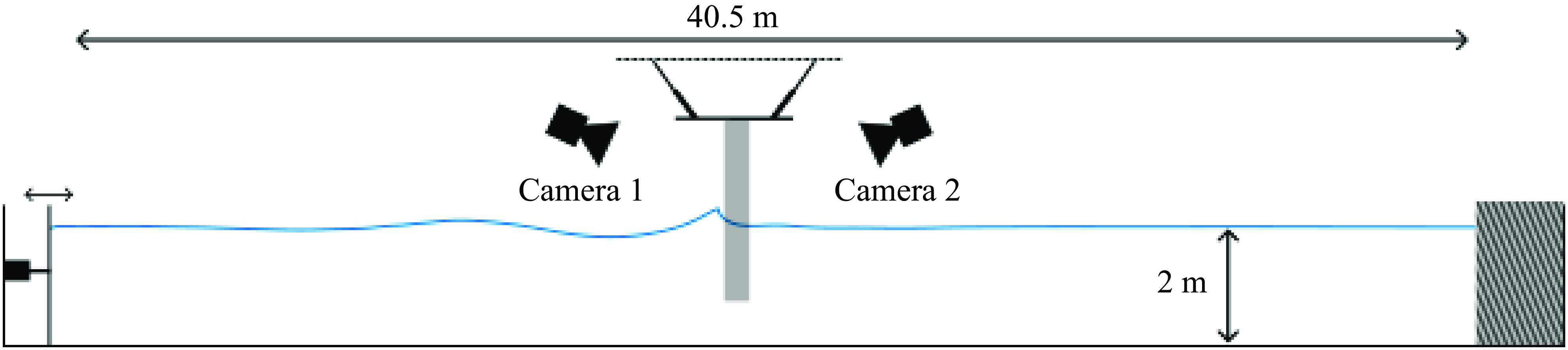
The experiments were carried out in the wave flume of Ifremer, Brest. A schematic description of the flume is depicted in figure 1. The experimental flume is 40.5 m long from the wave generator to the absorbing beach, 4 m wide and 2 m deep. It is equipped with a piston-type wave generator. The cylinder was fixed on a motion generator of type Mistral manufactured by Symétrie that allowed to accurately control the location of the cylinder. Two high-speed video cameras were installed on the side of the flume to film the front and rear faces of the cylinder during the wave impacts. The video cameras trigger was synchronised with the motion of the wave generator.
Scheme of the wave flume with the model and the high-speed video cameras.

Description of a breaking wave impacting the model in the flume. Parameter
 $\delta$
corresponds to the distance between the breaking location and the front face of the cylinder. The vertical dashed line indicates the breaking location
 $x_b$
and the horizontal dotted line the SWL.

A segmented model, of which a schematic view is depicted in figure 2, was used to measure independently the forces acting on different portions of the cylinder (sections
 $S_1$
to
 $S_4$
in figure 2). The model is a 1.81 m-high circular cylinder with a diameter of 40 cm. This diameter was chosen so as to be representative of an OWT with a mast diameter of 10 m at scale
 $1/25$
. Note that compared with the previous laboratory experiments that investigated the force induced by a breaking wave on a vertical cylinder, the present cylinder is within the models with the largest diameter, thus limiting the influence of unavoidable scale effects (due to aeration, surface tension or viscosity for instance). To the best of the authors’ knowledge, the sole experiments with a larger cylinder are the ones carried in the Great Wave Canal in Hanover (Irschik, Sparboom & Oumeraci Reference Irschik, Sparboom and Oumeraci2004; Wienke & Oumeraci Reference Wienke and Oumeraci2005). As shown in the cross-sectional view displayed in figure 3(
a), the cylinder is composed of six sections, out of which four are instrumented (sections
 $S_1$
to
 $S_4$
). Each instrumented section is composed of an outer part, called the skin element, and an inner part, called the backbone element. These two parts are visible in the exploded view depicted in figure 3(
b). The skin and backbone elements are linked through a load cell (of type MCS10-025 for sections
 $S_1$
,
 $S_2$
and
 $S_3$
and of type MCS10-010 for section
 $S_4$
). The signals of the load cells were recorded at a sample frequency of 250 kHz. Waterproofness of the model was ensured using surgical tape filling in the 3 mm gap between the different sections. The model was positioned so that the intersection between sections
 $S_4$
and
 $S_3$
lies at the still water level (SWL).
Description of the model.

With the present set-up, the distance to breaking,
 $\delta$
, was modified by changing the location of the cylinder, and not the breaking location of the wave as has been done by some authors in the past (e.g. Wienke & Oumeraci Reference Wienke and Oumeraci2005). This approach limits the variability of the impacting wave that is mainly due to the imperfect wavemaker motion repeatability and the variations of the water level induced by evaporation (Kimmoun, Ratouis & Brosset Reference Kimmoun, Ratouis and Brosset2010). On the other hand, a shift of the focal point in the wavemaker setpoint could have induced a slightly different shift of the breaking location due to nonlinear effects taking place during the wave propagation.
2.2. Compensation of the vibration induced force oscillations
During the impact of a breaking wave, different modes of the skin elements can be excited. This induces oscillations of the force signals that complicate the interpretation of the force measurements. In order to compensate for these oscillations, we applied the methodology proposed by Tassin et al. (Reference Tassin, Hulin and Jacques2024). In the aforementioned study, the present set-up was used as a case study to demonstrate the efficiency of the method. The results were limited to the upper section. Given that the methodology is detailed in Tassin et al. (Reference Tassin, Hulin and Jacques2024), we only recall the main assumptions of the method and we present the instrumentation used for the different sections.
The compensation methodology consists in recording the dynamic response of the impacted structure to estimate the part of the measured force that is induced by the structural response. The response is recorded by acceleration measurements at different points of the structure. Correction coefficients that were earlier computed from hammer tests are used to estimate the influence of the structural response on the force signal as the sum of the acceleration signals multiplied by the coefficients, and to subtract it from the raw measurement. With this methodology, we obtain an acceptable level of residual oscillations without losing the high-frequency content of the force signal (that would have been removed by a simple low-pass filter).
The number and locations of the accelerometers used for the present experiments are detailed in figure 4. Six accelerometers were placed on the upper section
 $S_1$
that is the one experiencing the most violent impacts, five were placed on section
 $S_2$
and one accelerometer per section was placed on sections
 $S_3$
and
 $S_4$
that were not impacted by the waves and experienced a limited level of oscillations. Similarly to the load cells, the accelerometers signals were recorded with a sampling frequency of 250 kHz. The number of accelerometers placed on a section determines the number of modes of the section that can be compensated for. For this reason, we filtered out the very high frequency content of the acceleration and force signals that is due to higher frequency modes. The force oscillations induced by these modes cannot be compensated for given the number of accelerometers used in the experiments. The signals recorded on section
 $S_1$
were low-pass filtered at 1000 Hz, the ones on section
 $S_2$
at 700 Hz and the ones on sections
 $S_3$
and
 $S_4$
at 300 Hz. Comparisons of the filtered and non-filtered frequency contents presented in Hulin (Reference Hulin2024) show that these cutoff frequencies retain most of the force frequency content. More details, in particular concerning the computation of the compensation coefficients, are also given in Hulin (Reference Hulin2024).
2.3. Definition of physical quantities of interest for the present study
In this section, we define different physical quantities that are used throughout the study.
The breaking location,
 $x_b$
, is defined as the location at which the free surface of the wave becomes locally vertical for the first time. We call the instant at which this event occurs the breaking time,
 $t_b$
. In figure 2, the blue profile corresponds to a wave profile at the instant
 $t_b$
. The breaking location,
 $x_b$
, is indicated by the vertical dashed line. The distance between the breaking location and the front face of the cylinder, also shown in figure 2, is denoted by
 $\delta$
. This distance is non-dimensionalised as
 $\bar \delta = \delta / L$
, where
 $L$
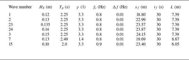
is the characteristic wavelength of the wave spectrum (see table 1). Here,
 $L$
is computed as the wavelength linked to the peak period
 $T_p$
of the spectrum through the linear dispersion relation (
 $L = {g T^2}\tanh ( {2 \pi h}/{L})/({2 \pi })$
, where
 $h$
is the water depth).
List of the parameters used to generate the breaking waves for the experimental campaign. The parameters of the JONSWAP spectrum are the significant wave height,
 $H_S$
, the peak period,
 $T_p$
, the peak enhancement factor,
 $\gamma$
, the cutoff frequency,
 $f_c$
, and the frequency discretisation,
 $\Delta f$
. Parameters
 $x_f$
and
 $t_f$
correspond to the focusing location and time, respectively. Parameter
 $L$
is the wavelength linked to the peak period
 $T_p$
through the linear dispersion relation.

Accelerometer configuration for the complete set-up: top view of the skin elements for sections
 $S_1$
(a),
 $S_2$
(b),
 $S_3$
(c) and
 $S_4$
(d).

Several seminal analytical approaches rely on the assumption that the force
 $F$
acting on a cylinder during a wave impact may be written as the sum of a drag term
 $F_D$
, an inertial term
 $F_I$
and a slamming term
 $F_S$
(Goda et al. Reference Goda, Haranake and Kitahata1966; Wienke & Oumeraci Reference Wienke and Oumeraci2005):
 \begin{equation} F = F_D + F_I + F_S. \end{equation}
However, as mentioned in § 1, extracting the slamming term
 $F_S$
from the total hydrodynamic force is not straightforward, partly because the load decomposition in (2.1) relies on an idealised representation of a breaking wave impact and because the slamming term will progressively evolve towards an inertial term as the cylinder penetrates the wave crest. As a consequence, many authors studied the hydrodynamic force acting on the whole cylinder (e.g. Paulsen et al. Reference Paulsen, Sonneville, Meulen and Jacobsen2019; Ma et al. Reference Ma, Tai, Dong and Perlin2020). Different possibilities were investigated by Ghadirian et al. (Reference Ghadirian, Pierella and Bredmose2023) to extract the impact term from the total hydrodynamic force obtained from numerical simulations. They observed that the different methods lead to rather different estimates of the slamming term. Moreover, some of the methods depend on the value of the first or even second time-derivative of the force and may not be applicable to experimental measurements affected by measurement noise. Sawaragi & Nochino (Reference Sawaragi and Nochino1984) approximated the impact force as the force acting above the SWL. This was permitted by the use of a segmented model. Even though a part of the hydrodynamic force acting above the SWL is due to the non-slamming terms, this definition has the advantage of being simple, unambiguous and applicable to experimental and numerical results. In the present study, we followed the approach of Sawaragi & Nochino (Reference Sawaragi and Nochino1984): we study the influence of the different impact conditions on the force
 $F_{\textit{SWL}}$
acting above the SWL. It corresponds to the force acting on the three upper sections
 $S_1$
,
 $S_2$
and
 $S_3$
(see figure 2). Another possibility would have been to study the force acting on the two upper sections, where the impact occurs. However, with this approach, the percentage of the wave height accounted for in the impact force would depend on the height of the wave. Moreover, non-slamming contributions may still be present in the measurements for some wave cases, while we may miss a part of the impact force for the stronger breaking waves.
Also, following Sawaragi & Nochino (Reference Sawaragi and Nochino1984), we define the non-dimensional impact force
 $\bar F_{\textit{SWL}}$
as
 \begin{equation} \bar F_{\textit{SWL}} = \frac {F_{\textit{SWL}}}{\pi \rho c^2 R \eta _b}, \end{equation}
where
 $R$
is the radius of the cylinder,
 $\rho$
the density of water,
 $c$
the wave crest celerity and
 $\eta _b$
the wave crest height. The quantity
 $\pi \rho c^2 R \eta _b$
corresponds to the theoretical maximum impact force acting on a cylinder of length
 $\eta _b$
entering calm water at speed
 $c$
derived from the theory of von Kármán (Reference von Kármán1929). Note that the non-dimensional impact force,
 $\bar F_{\textit{SWL}}$
, may be interpreted as the curling factor
 $\lambda$
introduced by Goda et al. (Reference Goda, Haranake and Kitahata1966) which represents the percentage of the wave crest that is impacting the cylinder. Indeed, following Goda’s theory, the maximum slamming force is equal to
 $F_S = \lambda \pi \rho c^2 R \eta _b$
. The difference between
 $\bar F_{\textit{SWL}}$
and
 $\lambda$
lies in the fact that
 $\bar F_{\textit{SWL}}$
includes all the force contributions acting above the SWL, while
 $\bar F_S = \lambda$
is the slamming term of the non-dimensional force.
3. Breaking waves generation and characterisation
The breaking waves were generated through the focusing of wave packets defined with a JONSWAP spectrum, using the iterative procedure detailed in Hulin et al. (Reference Hulin, Prevosto, Tassin, Filipot, Jacques and Grilli2025). The iterative procedure was applied to obtain breaking close to
 $x_t = 21$
m. Note that, in contrast to the work presented in Hulin et al. (Reference Hulin, Prevosto, Tassin, Filipot, Jacques and Grilli2025), the focusing time was selected as
 $t_f = 30$
s. During the experimental campaign, seven breaking wave cases were used. The parameters of the spectrum used for the wave generation are given in table 1. The significant wave height,
 $H_S$
, of the spectrum was varied to obtain different breaking strengths, i.e. different values of
 $\varGamma$
. The peak period,
 $T_p$
, was also varied to obtain breaking waves with different wavelengths. The focusing location,
 $x_f$
, results from the iterative procedure, and the wavelength
 $L$
is computed as the wavelength associated with the peak period of the spectrum,
 $T_p$
, through the linear dispersion relation (
 $L = {g T^2}\tanh ( {2 \pi h}/{L})/({2 \pi })$
, where
 $h$
is the water depth). For these waves, the ratio
 $h/L$
lies in the interval [0.23; 0.33], which is considered an intermediate water depth.
Numerical free-surface profiles at the instant of breaking of the waves listed in table 1. The waves are ordered by increasing values of
 $\varGamma$
and the index corresponds to the wave number (given in table 1). To improve the readability of the figure, the profiles were shifted in space so that the breaking location corresponds to
 $n \Delta$
, where
 $n$
is an integer and
 $\varDelta = 0.4$
m.

The different breaking waves were modelled using the two-dimensional FNPF solver based on the boundary element method proposed by Grilli et al. (Reference Grilli, Skourup and Svendsen1989) and Grilli & Subramanya (Reference Grilli and Subramanya1996). This model includes a wavemaker, the motion of which strictly corresponds to the motion of the physical wavemaker. The length of the NWT was fixed to 45 m. Given the short duration over which the waves propagate, it was deemed unnecessary to add a numerical absorbing zone at the end of the flume. The free-surface was discretised using 601 Lagrangian nodes, with an increased node density in the breaking zone. This discretisation was chosen so as to ensure the convergence of the
 $\varGamma$
values. The computation of the
 $\varGamma$
parameter requires to numerically differentiate the ratio
 $u/c$
, which itself is based on the numerical differentiation of the crest position. Consequently, the computation of
 $\varGamma$
is sensitive to the determination of the crest location and to the number of Lagrangian nodes close to the crest. Obtaining converged values of
 $\varGamma$
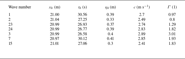
required significant efforts. The numerical details of the computations, a convergence study and a validation of the results through comparisons with experimental free-surface profiles are presented in Hulin et al. (Reference Hulin, Prevosto, Tassin, Filipot, Jacques and Grilli2025). The modelled free-surface profiles of the seven waves listed in table 1 are shown in figure 5. The waves are ordered by increasing values of
 $\varGamma$
and are shown at the instant of breaking. To improve the readability, the profiles are shifted in the
 $x$
-direction. Visually, it appears that the higher the value of
 $\varGamma$
, the higher the curling factor (the percentage of the wave that is ‘vertical’). The FNPF solver was also used to compute the different parameters of interest of the breaking waves given in table 2: the breaking location,
 $x_b$
, the instant of breaking,
 $t_b$
, the crest elevation at the instant of breaking,
 $\eta _b$
, the crest speed at the instant of breaking,
 $c$
, and the breaking strength parameter,
 $\varGamma$
. More details on the numerical configuration and the computation of the different wave parameters are given in Hulin et al. (Reference Hulin, Prevosto, Tassin, Filipot, Jacques and Grilli2025). The computation of the breaking location,
 $x_b$
, was used to compute the distance to breaking
 $\delta$
.
Characteristics of the breaking waves used during the experimental campaign.

In the following sections, we will observe that variations of a few centimetres of the distance to breaking may have a strong influence on the measured force. However, we are not able to assert that the values of
 $x_b$
listed in table 2 have a 1 cm accuracy. Indeed, experimental measurements of
 $x_b$
are not sufficiently accurate to be used as references to quantify the accuracy of the values of
 $x_b$
obtained numerically. Nevertheless, as explained in § 2.1, the distance
 $\delta$
was varied by modifying the position of the cylinder with the motion generator. The error on the position of the cylinder is known to be smaller than 1 mm. As a consequence, even if the absolute value of
 $\delta$
may be inaccurate, the variations of
 $\delta$
are very accurate. Thus, the obtained force evolutions as a function of
 $\delta$
are reliable, although the absolute values of
 $\delta$
are not known accurately.
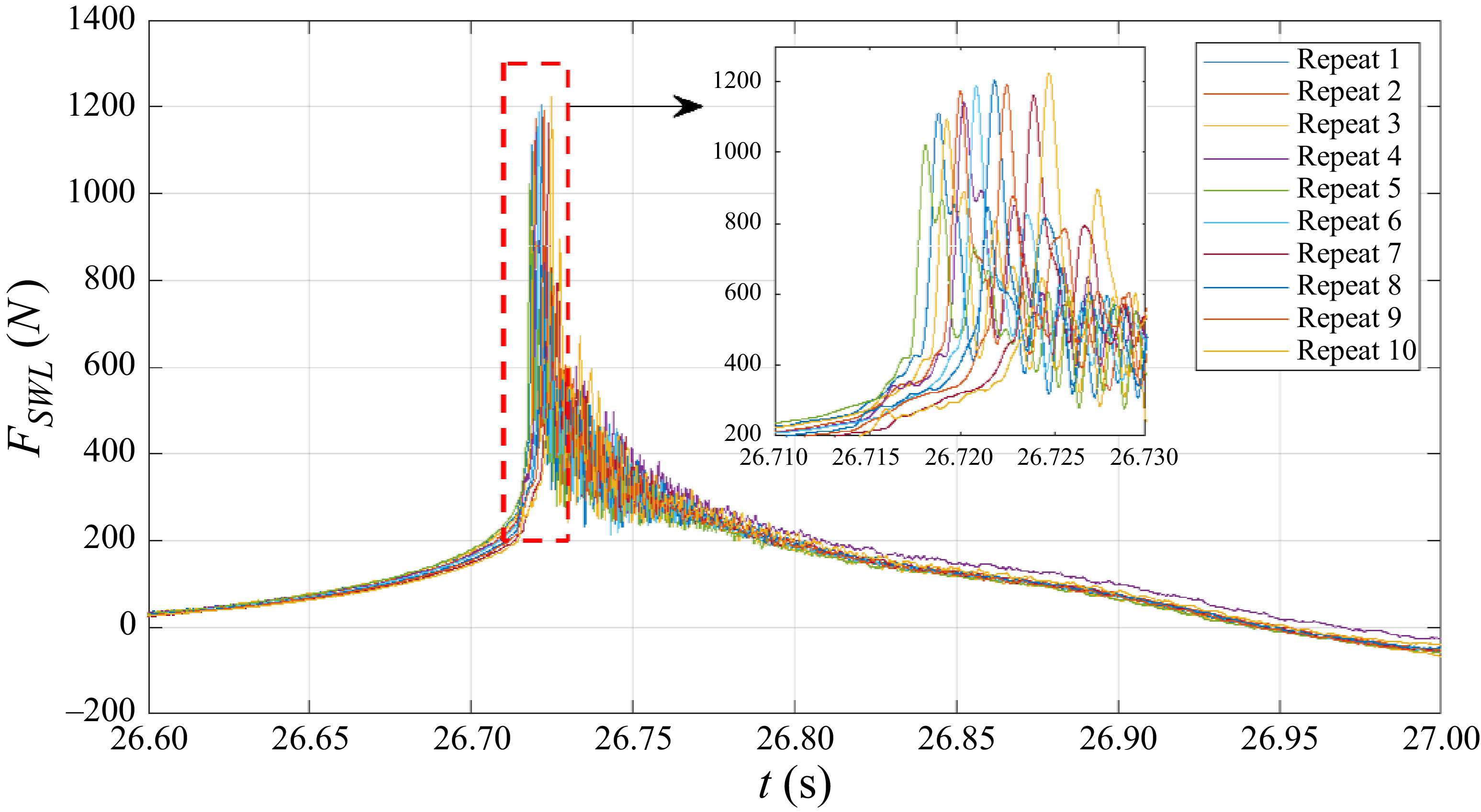
Time-histories of the force
 $F_{\textit{SWL}}$
measured during 10 repeats of the impact of wave 3 for
 $\bar \delta$
= 0.043. A zoomed-in view of the area in the red rectangle is also shown.

4. Time histories of the impact force for different wave impact conditions
In this section, we present the force measurements obtained for different impact conditions (i.e. different wave cases and locations of the cylinder). We investigate the repeatability of the force measurements in § 4.1 and we present the force measurements obtained for the different impact conditions in § 4.2. The effect of the wave shape on the characteristics of the force time-history is analysed in § 4.3. The importance of the diffraction of the wave by the cylinder for the force time-history is highlighted in § 4.4. In this section as well as in the following ones, the compensation methodology presented in § 2.2 is applied to the force measurements.
4.1. Repeatability of the force measurements
To assess the repeatability of the experiments, we repeated 10 times the force measurement for the impact of wave 3 at
 $\bar \delta$
= 0.043. These impact conditions were chosen because they are among those inducing the strongest loads and the highest levels of oscillations that we observed. As such, they are likely to be among the impact conditions with the lowest repeatability. The force measurements resulting from the 10 repeats are depicted in figure 6. The mean value of the maximum impact force for the 10 repeats is of 1151 N and it displays a standard deviation of 58 N, which represents 5 % of the mean value of the maximum impact force. It also appears from this figure that the force measurements are time shifted with respect to each other. The largest time shift, measured as the time interval between the force maxima for repeats five and 10, is of 7 ms (see the zoomed-in view in figure 6). This high level of repeatability was attained at the cost of a minimum resting time of 45 min between two experiments. In the following, the maximum value of the impact force in time will be called ‘magnitude of the impact force’. This term is used to differentiate it from the maximum over
 $\delta$
of the magnitude of the impact force.
Evolution of the time-histories of the force with the non-dimensional distance to breaking
 $\bar \delta$
for the different waves.

4.2. Force measurements for the different impact conditions
For the seven waves listed in table 1, the force
 $F_{\textit{SWL}}$
was measured for several distances to breaking
 $\delta$
. The corresponding time evolutions of
 $F_{\textit{SWL}}$
are shown in figure 7. Each panel corresponds to a wave case and each curve was obtained with a particular distance
 $\delta$
. The legends indicate the corresponding values of
 $\bar \delta$
. Note that intermediate
 $\bar \delta$
values, which are not shown in the figure for clarity, were also investigated. Except for waves 1 and 2 that displayed a much smaller variability in the force measurements, the experiments were repeated at least three times for almost all impact conditions the impacts of wave 23 at
 $\bar \delta = 0.097$
and
 $\bar \delta = 0.125$
were repeated only once. For a few impact conditions, more repeats (from four to 10) were carried out. Only one repeat is shown in figure 7 for the sake of clarity. The subpanels are ordered by increasing values of
 $\varGamma$
. Note that some 50 Hz oscillations due to electric noise are visible in figures 7(
b) and 7(e). This issue was fixed during the campaign, but some of the measurements are polluted.
It appears from figure 7 that, depending on the values of
 $\varGamma$
and
 $\delta$
, the impact force evolves from a non-impulsive to an impulsive regime. For instance, in figure 7(
g), the force time-history for
 $\bar \delta = 0.043$
is impulsive while the one for
 $\bar \delta = 0.003$
is not. However, for some conditions, it is not easy to assess whether the force is impulsive or not. For example, it is not clear if the force time-history corresponding to
 $\bar \delta = 0.016$
in figure 7(
g) should be considered as impulsive or not. Even if the presence of a dynamic response is linked to the impulsive nature of the force, this response is structure dependent; thus, it is not reliable to discriminate the impulsive nature of the excitation force based on the response of the structure.
For the waves with the smallest values of
 $\varGamma$
, namely waves 2 (
 $\varGamma = 0.8$
) and 1 (
 $\varGamma = 0.97$
), there is no value of
 $\bar \delta$
for which an impulsive increase of the measured force is observed (see figures 7
a and 7
b). For wave 2, the magnitude of the impact force slightly decreases when
 $\bar \delta$
increases, while it is rather constant for wave 1. This decrease is likely due to the modification of the shape of the wave due to breaking and to the wave propagation, while the non-dimensionalisation parameters (in particular the height of the crest at breaking,
 $\eta _b$
) are kept constant. For the other wave cases, corresponding to values of
 $\varGamma$
greater than one, some values of
 $\bar \delta$
lead to an impulsive force increase while others do not. Small values of
 $\bar \delta$
, i.e. close to zero, either present a small impulsive increase or are non-impulsive. Up to a value of
 $\bar \delta$
of approximately 0.05, the magnitude of the impact force
 $F_{\textit{SWL}}$
increases with
 $\bar \delta$
. The highest magnitude of
 $F_{\textit{SWL}}$
is reached for values of
 $\bar \delta$
in the interval
 $[0.04; 0.06]$
. The impacts for which
 $\bar \delta$
is in this interval are the ones showing the highest peak forces and the shortest rising times. For larger values of
 $\bar \delta$
, the magnitude of
 $F_{\textit{SWL}}$
slowly decreases. It will be shown in the following sections that the wave impacts with values of
 $\bar \delta$
higher than 0.06 correspond to the impact of significantly overturned waves for which a jet is formed.
4.3. Shape of the wave at impact for different distances to breaking
It appeared in the previous section that different distances to breaking, i.e. different wave shapes at impact, may lead to very different force time-histories. This section is devoted to the influence of the wave shape at impact on the characteristics of the force time-history. The shape of wave 3 at the instant of maximum force for different distances to breaking is illustrated in figure 8 with high-speed video camera images. These instants are indicated by the red dots shown in figure 7(
g). The wave profiles obtained with the FNPF solver at the same instant are shown for comparison. The solid vertical line superimposed to the numerical profile indicates the position of the front face of the cylinder. For values of
 $\bar \delta$
higher than 0.084, the numerical free-surface profiles are not shown because they are not available at the instant of maximum force (the FNPF simulations stop when the tongue of the crest touches the water bulk). Note that the numerical free-surface profiles depicted in figure 7(
g) were time shifted of 20 ms. As discussed in Hulin (Reference Hulin2024), this time shift allowed to compensate for the delay between the experimental and numerical wave profiles. The images depicted in figure 7(
g) show that for
 $\bar \delta$
values higher than 0.043 (figure 8
d and below), the tongue of the wave has already reached the cylinder at the instant of maximum force. This is confirmed by the numerical free-surface profiles. It is likely that the impact of the tongue on the cylinder is responsible for the rather rapid but smaller force increases prior to the main impulse visible on the force time-histories of the impact of wave 3 depicted in figure 7(
g). These increases occur for
 $\bar \delta = 0.043$
and higher values. The black vertical dashed lines indicate the time instants at which these first force increases are observed. The fact that two different impacts (of the wave tongue and vertical front) occur when the wave crest has overturned is also supported by the studies of Zhou et al. (Reference Zhou, Chan and Melville1991), Chan, Cheong & Tan (Reference Chan, Cheong and Tan1995), Manjula et al. (Reference Manjula, Sannasiraj and Palanichamy2013) and Govindasamy et al. (Reference Govindasamy, Chella, Sannasi and Rajamanickam2023), who reported the appearance of two pressure peaks for wave impacts with high values of
 $\bar \delta$
.
Images of wave 3 impacting the model for various values of
 $\bar \delta$
. All the images are taken at the instant at which the impact load is maximum. The plot in the upper left corner corresponds to the numerical free-surface profile at the same instant. The solid vertical line indicates the position of the front face of the cylinder. The dashed vertical line indicates the position of the locally vertical front.

It also appears in figure 8 that at the instant of maximum force, the locally vertical part of the wave, which position is indicated by the dashed vertical line, is still far from the front face of the cylinder. In the basin, the wave profile is modified by the presence of the cylinder. It is likely that this modification is such that at the instant of maximum force, the locally vertical front indeed reaches the front face of the cylinder in the basin.
4.4. Influence of wave diffraction on the force time-histories
In § 4.2, we observed that impact conditions with small values of
 $\varGamma$
or values of
 $\bar \delta$
close to zero do not lead to an impulsive force increase although the profile of the undisturbed wave presents a vertical front when it reaches the location of the cylinder. It is likely that this phenomenon is due to the fact that the shape of the wave is affected by the presence of the cylinder prior to the impact. This modification of the wave profile in the vicinity of the cylinder can indeed be observed on the high-speed video camera images. For the cases that do not show an impulsive increase of the force, we observe the appearance of a run-up that prevents the vertical front of the wave from impacting the cylinder. This is illustrated in figure 9 which presents images taken during two impacts of wave 24 with different values of
 $\bar \delta$
. The images in subpanels (i) correspond to
 $\bar \delta = 0.016$
and the images in subpanels (ii) to
 $\bar \delta = 0.043$
. It can be seen in figure 7(
d) that
 $\bar \delta = 0.016$
does not lead to an impulsive force increase while
 $\bar \delta = 0.043$
does. In figure 9, the images in the first raw (figure 9
a) were taken 10 ms before the measured force reaches its maximum value, the images in the second raw (figure 9
b) at the instant
 $t_{\textit{max}}$
(when the force is maximum) and the images in the third raw (figure 9
c) 10 ms after
 $t_{\textit{max}}$
. The run-up is already visible 10 ms before the maximum force is reached for the non-impulsive case
 $\bar \delta = 0.016$
(see the blue arrow in figure 9
a) while it is not for the impulsive case
 $\bar \delta = 0.043$
. At the instant of maximum force (figure 9
b), the extent of the run-up has increased for the case
 $\bar \delta = 0.016$
while the wetted surface expansion is not yet visible for the case
 $\bar \delta = 0.043$
. The extent of the cylinder surface affected by the run-up is strongly increased 10 ms after the instant of maximum force (figure 9
c) for the non-impulsive case while the fragmentation of the jet visible in figure 9(
cii) indicates that a hydrodynamic impact occurred.
Images of the impact of wave 24 on the vertical cylinder at different instants around the instant of the maximum force
 $t_{\textit{max}}$
. Subpanels (i) correspond to
 $\bar \delta = 0.016$
while subpanels (ii) correspond to
 $\bar \delta = 0.043$
.

These images show that the presence of the structure may modify the wave in such a way that the impact of the wave front is hindered. For waves 1 and 2, which correspond to low values of
 $\varGamma$
and for which no value of
 $\bar \delta$
leads to an impulsive force increase, a similar run-up was observed. One may also expect that in certain cases for which the wave front impacts the cylinder, the force evolution may be affected by wave diffraction effects. This assumption is supported by the results of Batlle Martin et al. (Reference Martin, Marc, Jeffrey, Filipot, Hulin, Tassin and Renaud2023) who observed through numerical simulations that the vertical part of a wave that may induce impact is reduced when the diameter of the cylinder is increased. The importance of the wave diffraction was also highlighted by Chan & Melville (Reference Chan and Melville1989) who measured the impact forces induced by breaking waves impacting on a vertical circular cylinder and a vertical wall. They observed that a vertical wall, which corresponds to the case of a cylinder with an infinite diameter, has a greater influence on the development of the breaking wave than a cylinder. In the present experiments, the radius of the cylinder was kept constant, but waves of different sizes were investigated. More precisely, the ratio
 $R/L$
between the radius of the cylinder and the characteristic wavelength of the impacting wave is ranging from
 $2.3 \times 10^{-2}$
to
 $3.3 \times 10^{-2}$
, with five out of seven waves corresponding to
 $R/L=2.7\times 10^{-2}$
. These values were chosen so as to be representative of the wave conditions that may be experienced by a spar-type wind turbine floater. Given the rather limited range of values, it has not been possible to characterise the influence of the
 $R/L$
ratio on the perturbation of the wave front and on the resulting impact force. As a consequence, one should keep in mind that the non-dimensional force measurements presented in the following sections may not be valid for impact conditions where the ratio
 $R/L$
is significantly different from the ones used in the present study.
5. Influence of the impact conditions on the magnitude of the impact force
5.1. Evolution of the magnitude of the impact force with the impact conditions
In the present section, we investigate the influence of the impact conditions, i.e. of the values of
 $\bar \delta$
and
 $\varGamma$
, on the magnitude of the impact force. As a reminder, the term ‘magnitude of the impact force’ denotes the maximum value over time reached by the measured force
 $F_{\textit{SWL}}$
. For wave 3, the magnitude of the impact force obtained for different values of
 $\bar \delta$
is indicated by the red dots shown in figure 7(
g). The magnitude of the impact force obtained for each impact condition and each repeat is reported in figure 10. Each colour is associated with a particular wave. In accordance with the observations of § 4, for the smaller values of
 $\varGamma$
(
 $\varGamma \lt 1$
for waves 1 and 2), the magnitude of the impact force is almost independent of the value of
 $\bar \delta$
. For higher values of
 $\varGamma$
, the maximum value of the impact force magnitude is reached close to
 $\bar \delta = 0.05$
. For these five wave cases with
 $\varGamma \gt 1$
, the increase of the force prior to the peak is steeper than the subsequent decrease. It is also interesting to note that waves 15, 7 and 24, whose values of
 $\varGamma$
are around 1.9, present rather close evolutions for the magnitude of the non-dimensional impact force.
Evolution of the magnitude of the non-dimensional force
 $\bar F_{\textit{SWL}}$
as a function of
 $\bar \delta$
. In the legend, the
 $\varGamma$
indices correspond to the wave numbers given in table 2. The red dots, shown only for wave 3, correspond to the mean value of the impact force magnitude over the different repeats of the same impact conditions.

5.2. Maximum impact force induced by a given wave
As observed in the previous section, the magnitude of the impact force generated by a given wave depends on the distance to breaking
 $\delta$
. In the present section, the focus is on the maximum of the magnitude of the impact force that may be reached for a given wave and its evolution as a function of
 $\varGamma$
.
For each impact condition, i.e. each couple (
 $\varGamma , \bar \delta$
), we compute the mean value of the impact force magnitude, denoted by
 $\bar F_{\textit{SWL}}^{mean}$
, over the different repeats of the experiment. The values of
 $\bar F_{\textit{SWL}}^{mean}$
obtained for the different values of
 $\bar \delta$
for wave 3 (
 $\varGamma = 3.01$
) are represented in figure 10 by red dots. It appears that there is a value of
 $\bar \delta$
for which
 $\bar F_{\textit{SWL}}^{mean}$
is maximum. This maximum impact force, that is illustrated by the blue arrow in figure 10, is denoted by
 $\bar F_{\textit{SWL}}^{\textit{max}}$
.
Evolution of the maximum impact force
 $\bar F_{\textit{SWL}}^{\textit{max}}$
as a function of
 $\varGamma$
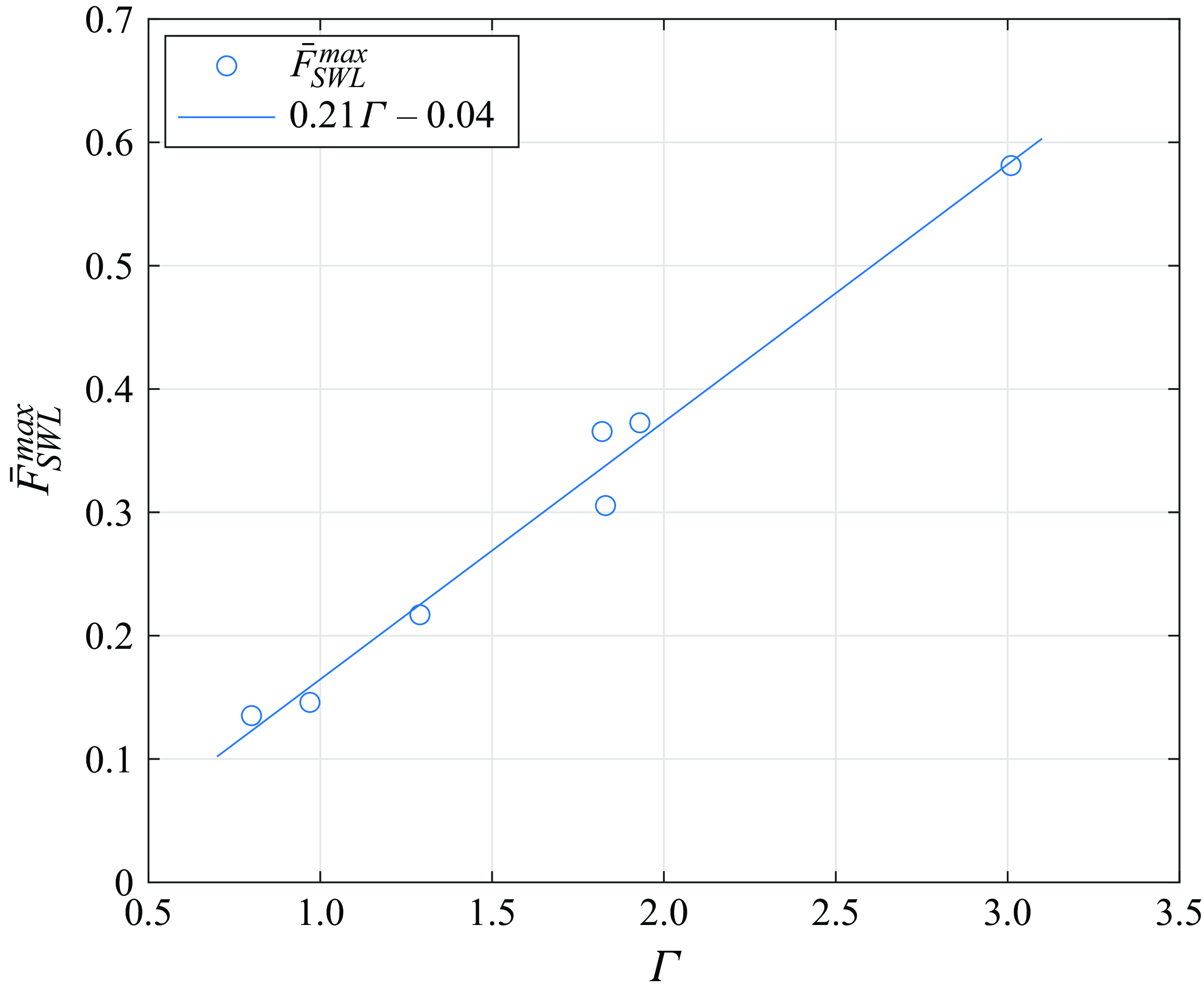
. Each circle corresponds to the maximum impact force obtained for a wave case. The solid line is a linear approximation of the evolution of
 $\bar F_{\textit{SWL}}^{\textit{max}}$
as a function of
 $\varGamma$
.

The evolution of
 $\bar F_{\textit{SWL}}^{\textit{max}}$
as a function of
 $\varGamma$
is depicted in figure 11. Each circle corresponds to a wave case and the solid line is a linear approximation of the evolution of
 $\bar F_{\textit{SWL}}^{\textit{max}}$
. The results presented in figure 11 show that the maximum non-dimensional impact force
 $\bar F_{\textit{SWL}}^{\textit{max}}$
is strongly correlated to the breaking strength
 $\varGamma$
. This is an important outcome of the present study. Note also that the circles corresponding to waves 7, 15 and 24 lie close to each other in figure 11. These three waves have different wavelengths ranging from 6.05 m to 8.67 m and wave heights ranging from 0.30 m to 0.41 m, but they are all mild plunging breakers with a value of
 $\varGamma$
of approximately 1.8. The present results thus suggest that the evolution of
 $\bar F_{\textit{SWL}}^{\textit{max}}$
is independent of the wave scale in the range of values studied here.
Note that the systematic variation of the values of
 $\delta$
that was carried out is of prime importance for the results presented in figure 11. Indeed, for wave 3 for instance, if
 $\bar F_{\textit{SWL}}^{\textit{max}}$
had been estimated at a
 $\delta$
value 20 cm smaller than the one leading to
 $\bar F_{\textit{SWL}}^{\textit{max}}$
, the maximum force would have been underestimated by 30 %. In figure 7(
g), this would correspond to estimating
 $\bar F_{\textit{SWL}}^{\textit{max}}$
with the curve labelled
 $\bar \delta =$
0.030 instead of the curve labelled
 $\bar \delta =$
0.057. The value obtained for
 $\bar F_{\textit{SWL}}^{\textit{max}}$
would thus be close to the one obtained for wave 24. Studying the influence of the distance to breaking
 $\delta$
on the impact force appears as an important step in the determination of the maximum impact force
 $\bar F_{\textit{SWL}}^{\textit{max}}$
that may be induced by a breaking wave.
The present force measurements can be compared with those of Sawaragi & Nochino (Reference Sawaragi and Nochino1984) that used a similar approach: they investigated the force acting above the SWL for several values of
 $\bar \delta$
and they used the same non-dimensionalisation factor, namely
 $\pi \rho c^2 R \eta _b$
. However, the wave generation procedure is not sufficiently detailed to numerically reproduce the breaking waves and compute the value of the
 $\varGamma$
parameter. Nevertheless, it is possible to compare the typical values of the non-dimensional force for different kinds of breaking waves. For the wave that is described as spilling, they obtained a maximum non-dimensional impact force
 $\bar F_{\textit{SWL}}^{\textit{max}}$
of approximately 0.2. This value is reasonably close to the values of 0.15 and 0.14 obtained in the present study for the spilling waves 1 and 2. For the wave that is described as plunging, they obtained
 $\bar F_{\textit{SWL}}^{\textit{max}} = 0.9$
. This value is higher than the value of 0.58 obtained for wave 3. It is possible that their plunging wave is more energetic than wave 3. Also note that their results present a significant scatter.
5.3. Parametrisation of the maximum impact force as a function of
 $\bar \delta$

Evolution of the magnitude of the non-dimensional impact force as a function of
 $\bar \delta$
. In the legend, the
 $\varGamma$
indices correspond to the wave numbers given in table 2. For each wave, the solid line corresponds to the result of the fit obtained with the parametric function of (5.1).

Considering the evolution of the non-dimensional force
 $\bar F_{\textit{SWL}}$
as a function of
 $\bar \delta$
that was described in § 5.1, we propose to fit the force evolution for each wave using two Gaussian functions. One function describes the increase of the magnitude of the force prior to its peak and the other one describes the subsequent decrease. Using two functions allows us to account for the fact that the increase of the force magnitude is faster than its subsequent decrease. In addition, a constant
 $\bar F_0$
is added to the fit to account for the fact that the force magnitude does not seem to tend to zero for negative and high values of
 $\bar \delta$
. For waves 1 and 2, for which the magnitude of the force is almost independent of
 $\bar \delta$
, we only identify this constant parameter. Consequently, for waves 1 and 2, this constant corresponds to the mean value of the magnitude of the impact force obtained for the different impact conditions. For the other waves, the parametric function writes as
 \begin{equation} f(\bar \delta ) = \bar F_0 + \bar F_G\exp \left (-\frac {1}{2}\frac {(\bar \delta -\bar \delta _{\textit{max}})^2}{\sigma ^2}\right ),\quad \textrm { with } \begin{cases} \sigma = \sigma _l &\text{if}\, \bar \delta \lt \bar \delta _{\textit{max}}\\ \sigma = \sigma _r &\text{if}\, \bar \delta \gt \bar \delta _{\textit{max}} \end{cases}. \end{equation}
This function depends on five parameters, which can be interpreted as follows. Parameters
 $\bar F_0$
and
 $\bar F_G$
describe the magnitude of the impact force:
 $\bar F_0$
is the part that does not depend on
 $\bar \delta$
and
 $\bar F_G$
is the multiplicative coefficient for the asymmetric Gaussian function that accounts for the dependence of the force on
 $\bar \delta$
. Parameter
 $\bar \delta _{\textit{max}}$
is the value of
 $\bar \delta$
for which the fit reaches its maximum, i.e. the value of
 $\bar \delta$
for which the most severe impact is obtained. Therefore, the maximum value of the impact force magnitude corresponds to
 $\bar F_{\textit{SWL}}|_{\bar \delta _{\textit{max}}} = \bar F_0 + \bar F_G$
. Parameters
 $\sigma _l^2$
and
 $\sigma _r^2$
characterise the range of values of
 $\bar \delta$
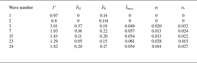
over which the magnitude of the impact force rapidly increases and decreases. The obtained fits of the force evolutions are depicted in figure 12, along with the experimental measurements. The values obtained for the parameters of the fits are given in table 3 for the seven wave cases.
Parameters of the Gaussian fits for the different waves.

The evolution of the parameters
 $\bar F_G$
and
 $\bar F_0$
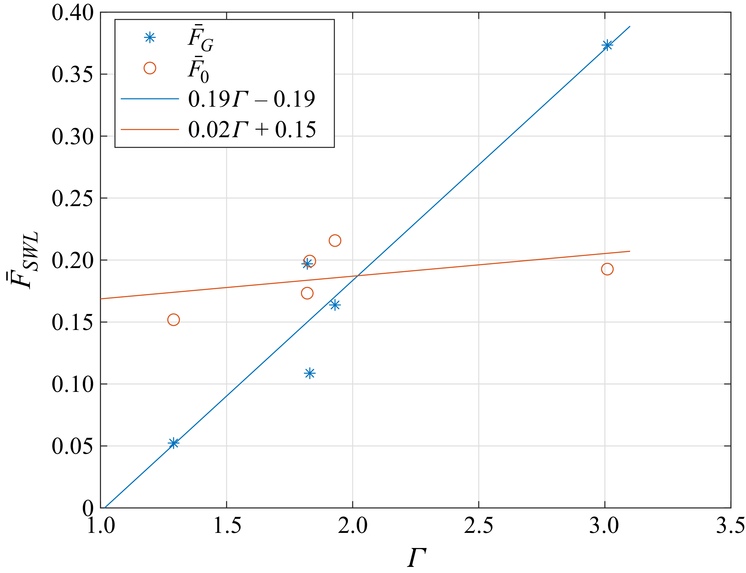
that were obtained for waves 3, 7, 15, 24 and 23 are shown in figure 13 as a function of
 $\varGamma$
. The solid lines correspond to linear interpolations of these two quantities and each marker corresponds to a wave case. It appears that parameter
 $\bar F_G$
strongly increases when
 $\varGamma$
increases. The dependence of
 $\bar F_0$
on
 $\bar \delta$
is much less pronounced. The mean value of
 $\bar \delta _{\textit{max}}$
obtained for waves 3, 7, 15, 24 and 23 is 0.055, which means that
 $\delta _{\textit{max}}$
corresponds to 5.5 % of the wavelength of the impacting wave. This is in close agreement with the value of 6 % of the wavelength obtained in the study by Sawaragi & Nochino (Reference Sawaragi and Nochino1984). To the best of the authors’ knowledge, the study by Sawaragi & Nochino (Reference Sawaragi and Nochino1984) is the only one giving an estimate of
 $\bar \delta _{\textit{max}}$
. Nevertheless, other studies (e.g. Ma et al. Reference Ma, Tai, Dong and Perlin2020; Zhang et al. Reference Zhang, Xiao, Cheng, Wei and Chen2024) observed that the strongest impact loads were obtained for the impact of an overturned wave, the tongue of which has not impinged the free surface yet. This is also in agreement with the value of
 $\bar \delta _{\textit{max}}$
obtained in the present study. Indeed, an image of wave 3 for which
 $\bar \delta \approx \bar \delta _{\textit{max}}$
is depicted in figure 8(
e) at the instant of maximum force. It corresponds to a significantly overturned wave, the tongue of which has not impinged the free surface yet.
Evolution of parameters
 $\bar F_0$
and
 $\bar F_G$
as a function of
 $\varGamma$
.

6. Conclusions
We quantitatively investigated the influence of the distance to breaking and of the breaking strength on the force generated by a breaking wave impacting a segmented vertical cylinder. The strength of the breaking wave was characterised by the
 $\varGamma$
parameter introduced by Derakhti et al. (Reference Derakhti, Banner and Kirby2018). The distance to breaking was computed as the distance between the front face of the cylinder and the breaking location. Our analysis is based on the force measured above the SWL. Seven different wave cases displaying various breaking strengths
 $\varGamma$
were investigated. The distance
 $\delta$
was systematically varied for the seven wave cases. The values of the parameters
 $\delta$
and
 $\varGamma$
were estimated using a FNPF solver. The compensation methodology proposed in Tassin et al. (Reference Tassin, Hulin and Jacques2024) was used to reduce the amplitude of the force oscillations induced by the dynamic structural response of the model.
For each wave case, the time histories of the impact forces obtained for different values of
 $\delta$
are presented. It appears that for values of
 $\varGamma$
lower than one, no position of the cylinder leads to an impulsive force. The first wave case inducing a hydrodynamic impact corresponds to a value of
 $\varGamma = 1.29$
. For higher values of
 $\varGamma$
, the higher the value of
 $\varGamma$
, the stronger the impact force. Thanks to the high-speed video camera images, we highlighted that the absence of hydrodynamic impact for some wave cases and some values of
 $\delta$
is a consequence of the presence of a run-up that hinders the impact of the wave front on the cylinder. We observed that the maximum value of the impact force magnitude is linearly related to the
 $\varGamma$
parameter. The evolution of the magnitude of the impact force with the non-dimensional distance to breaking
 $\bar \delta$
is as follows: it increases until it reaches a peak value for
 $\bar \delta \approx 0.05$
; then, a slower decrease is observed.
The conclusions of this work are based on a compilation of more than 180 impact experiments. Nevertheless, several limitations of the present study were identified and could be improved in future works. First, only seven breaking wave cases were exploited, out of which two did not induce hydrodynamic impact. This limitation is related to the important experimental time required to vary the distance to breaking
 $\delta$
for each wave case. Moreover, it is necessary to wait for 45 min between two consecutive tests to ensure that the flume is at rest. This ensures a good repeatability of the measurements (
 $\approx 5$
% variations on the magnitude of the force), but it is at the expense of the number of impact conditions that could be investigated. This reduced number of waves is not sufficient to investigate the influence of the scale of the wave on the impact force. As mentioned in § 4.4, we observed that the run-up influences the presence of hydrodynamic impact. It is thus likely that it also influences the magnitude of the impact force. This has indeed been shown numerically by Batlle Martin et al. (Reference Martin, Marc, Jeffrey, Filipot, Hulin, Tassin and Renaud2023). The importance of the run-up is likely driven by the ratio between the wavelength of the impacting wave and the radius of the cylinder. As such, it would be of interest to extend the present study to breaking waves of different sizes or to cylinders of different sizes. Another difficulty that was encountered during the study is the computation of the
 $\varGamma$
parameter. Indeed, we had to rely on numerical simulations to estimate the value of
 $\varGamma$
for the different wave cases. Ideally, this quantity should be estimated experimentally, but this would require significant developments without guaranties of success. Indeed, the computation of
 $\varGamma$
from numerical results is already delicate (see Hulin et al. Reference Hulin, Prevosto, Tassin, Filipot, Jacques and Grilli2025), so computing
 $\varGamma$
from experimental results is expected to be even more difficult because of inherent measurement uncertainties (such as signal noise). Lastly, scale effects (due to the influence of the aeration, the surface tension or the water viscosity for instance) were not investigated in the present study.
Acknowledgements
F.H. gratefully acknowledges the support of S. Grilli that furnished the FNPF solver used to model the breaking waves. F.H. and A.T. are grateful to M. Laurent from Ifremer for his contribution to the design of the segmented model, and to the technical team of Ifremer for their support during the experimental campaign.
Funding
This work is performed under financial support of grant ANR10IEED-0006-34, France Energies Marines project DIMPACT (Dimensionnement d’éoliennes flottantes prenant en compte les impacts de la raideur et du déferlement des vagues).
Declaration of interests
The authors report no conflict of interest.
Data availability statement
The data that support the findings of this study are openly available in the SeaNoe database under the name ‘Breaking wave impact loads on a cylinder: model-scale experimental measurements and wave simulations from the DIMPACT project’ at https://doi.org/10.17882/110481. See the Journal of Fluid Mechanics’ research transparency policy for more information.