1 Introduction
Wake meandering, a large-scale coherent motion of the turbine wake, has considerable effects on the velocity deficit and turbulence intensity in the wake. It is of major significance for maximising wind farm power production and reducing aeroelastic loads on downwind turbines. However, the mechanism of wake meandering is still not well understood, and reduced-order engineering models cannot take the wake meandering effects into account accurately. Recent studies of wake meandering have concentrated on laboratory-scale turbines (Iungo et al.
Reference Iungo, Viola, Camarri, Porté-Agel and Gallaire2013; Kang, Yang & Sotiropoulos Reference Kang, Yang and Sotiropoulos2014; Foti et al.
Reference Foti, Yang, Guala and Sotiropoulos2016). Okulov et al. (Reference Okulov, Naumov, Mikkelsen, Kabardin and Sørensen2014), employing a model turbine, found that a regular Strouhal number
 $St=fD/U\approx 0.23$
(where
 $f$
is a frequency,
 $D$
is the turbine diameter and
 $U$
is the incoming velocity) exists in the turbine wake under different operating and inflow conditions. Visualisations revealed that the wake far from the turbine oscillates with the precession of a helical vortex. However, the study was unable to ascertain whether inflow turbulence has an effect on the frequency or amplitudes in the wake meandering. Moreover, it is unclear whether the Strouhal number similarity remains at utility scale and field operating conditions. There have been field and numerical studies of utility-scale turbines (Whale et al.
Reference Whale, Anderson, Bareiss and Wagner2000; Aitken et al.
Reference Aitken, Banta, Pichugina and Lundquist2014; Berg et al.
Reference Berg, Bryant, LeBlanc, Maniaci, Naughton, Paquette, Resor, White and Kroeker2014). However, the field-based studies remain difficult to perform, partly attributed to the lack of controllability in measurements. Challenges also exist in obtaining high-fidelity computational results across a range of rotor sizes and temporal scales. Owing to these limitations, wake meandering at the utility scale has yet to be fully characterised and understood. It is unclear, for instance, whether we can directly apply the knowledge obtained from laboratory-scale studies to optimise utility-scale wind farm deployment and operation because of the different incoming wind conditions, turbine designs and operating conditions. In this study, we attempt to bridge this knowledge gap by carrying out large-eddy simulation (LES) to investigate wake meandering for four different turbines with rotor diameters spanning nearly three orders of magnitude: from the laboratory scale with a rotor diameter of 0.128 metres to utility scale with a rotor diameter of 96 m.
In numerical simulations, turbines are usually parametrised as actuator disks (Yang, Kang & Sotiropoulos Reference Yang, Kang and Sotiropoulos2012) or actuator lines (Sørensen & Shen Reference Sørensen and Shen2002; Troldborg, Sorensen & Mikkelsen Reference Troldborg, Sorensen and Mikkelsen2010; Yang et al. Reference Yang, Sotiropoulos, Conzemius, Wachtler and Strong2015b ; Abkar & Dabiri Reference Abkar and Dabiri2017). However, such parametrisations cannot resolve the energetic coherent structures induced by the turbine nacelle (Iungo et al. Reference Iungo, Viola, Camarri, Porté-Agel and Gallaire2013; Kang et al. Reference Kang, Yang and Sotiropoulos2014; Foti et al. Reference Foti, Yang, Guala and Sotiropoulos2016), which have been shown to affect the intensity of wake meandering in the far wake. Geometry-resolving simulations can capture the geometric characteristics of the wind turbine and accurately predict the wake meanderings. However, geometry-resolving simulations are extremely expensive, especially for wake meandering simulations for which the low-frequency modes of wake meandering have to be captured. In this study, a new actuator surface model for the turbine blades and nacelle developed by Yang & Sotiropoulos (Reference Yang and Sotiropoulos2018), which has been successfully applied to different turbine designs, is employed to parametrise the turbine. This model is able to accurately capture the details of the near-wake flow and resolve the intensity of wake meandering on a grid resolution similar to that employed in standard actuator line simulations.
In this work, we seek to investigate the similarity of wake meandering characteristics at far-wake locations for turbines spanning three orders of magnitude in size. Similar Strouhal numbers of wake meandering have been observed in the literature for laboratory-scale turbines (Okulov & Sørensen Reference Okulov and Sørensen2007; Medici & Alfredsson Reference Medici and Alfredsson2008; Chamorro et al. Reference Chamorro, Hill, Morton, Ellis, Arndt and Sotiropoulos2013; Okulov et al. Reference Okulov, Naumov, Mikkelsen, Kabardin and Sørensen2014; Howard et al. Reference Howard, Singh, Sotiropoulos and Guala2015b ; Foti et al. Reference Foti, Yang, Guala and Sotiropoulos2016). We will show for the first time that Strouhal number similarity holds for different turbine designs across a broad range of turbine rotor diameters. We also employ the spatio-temporal filtering technique proposed by Foti et al. (Reference Foti, Yang, Guala and Sotiropoulos2016) to reconstruct wake meanders from the three-dimensional flow fields, and propose suitable velocity and length scales for various quantities characterising wake meandering.
2 Numerical methods
The governing equations are the spatially filtered unsteady three-dimensional incompressible Navier–Stokes and continuity equations. The governing equations are discretised on a hybrid staggered/non-staggered grid using three-point central finite differencing and integrated in time via a second-order-accurate fractional step method. In compact tensor notation (repeated indices imply summation), the continuity and momentum equations are as follows (
 $i,j=1,2,3$
):
 $$\begin{eqnarray}\displaystyle \hspace{-10.00002pt} & \displaystyle J\frac{\unicode[STIX]{x2202}U^{i}}{\unicode[STIX]{x2202}\unicode[STIX]{x1D709}^{i}}=0, & \displaystyle\end{eqnarray}$$
 $$\begin{eqnarray}\displaystyle \hspace{-10.00002pt} & \displaystyle \frac{1}{J}\frac{\unicode[STIX]{x2202}U^{i}}{\unicode[STIX]{x2202}t}=\frac{\unicode[STIX]{x1D709}_{l}^{i}}{J}\left(-\frac{\unicode[STIX]{x2202}}{\unicode[STIX]{x2202}\unicode[STIX]{x1D709}^{j}}(U^{j}u_{l})+\frac{\unicode[STIX]{x1D707}}{\unicode[STIX]{x1D70C}}\frac{\unicode[STIX]{x2202}}{\unicode[STIX]{x2202}\unicode[STIX]{x1D709}^{j}}\left(\frac{\unicode[STIX]{x1D628}^{jk}}{J}\frac{\unicode[STIX]{x2202}u_{l}}{\unicode[STIX]{x2202}\unicode[STIX]{x1D709}^{k}}\right)-\frac{1}{\unicode[STIX]{x1D70C}}\frac{\unicode[STIX]{x2202}}{\unicode[STIX]{x2202}\unicode[STIX]{x1D709}^{j}}\left(\frac{\unicode[STIX]{x1D709}_{l}^{j}p}{J}\right)-\frac{1}{\unicode[STIX]{x1D70C}}\frac{\unicode[STIX]{x2202}\unicode[STIX]{x1D70F}_{lj}}{\unicode[STIX]{x2202}\unicode[STIX]{x1D709}^{j}}+F_{l}\right)\!, & \displaystyle\end{eqnarray}$$
where
 $\unicode[STIX]{x1D709}_{l}^{i}=\unicode[STIX]{x2202}\unicode[STIX]{x1D709}^{i}/\unicode[STIX]{x2202}x_{l}$
are the transformation metrics,
 $J$
is the Jacobian of the geometric transformation,
 $u_{i}$
is the
 $i$
th component of the velocity vector in Cartesian coordinates,
 $U^{i}=(\unicode[STIX]{x1D709}_{m}^{i}/J)u_{m}$
is the contravariant volume flux,
 $\unicode[STIX]{x1D628}^{jk}=\unicode[STIX]{x1D709}_{l}^{j}\unicode[STIX]{x1D709}_{l}^{k}$
are the components of the contravariant metric tensor,
 $\unicode[STIX]{x1D70C}$
is the density,
 $\unicode[STIX]{x1D707}$
is the dynamic viscosity,
 $p$
is the pressure and
 $\unicode[STIX]{x1D70F}_{ij}$
represents the anisotropic part of the subgrid-scale stress tensor. A body force
 $F_{l}$
is used to account for the forces exerted by the actuator-based model. A dynamic Smagorinsky model (Smagorinsky Reference Smagorinsky1963) developed by Germano et al. (Reference Germano, Piomelli, Moin and Cabot1991) is used for closure for
 $\unicode[STIX]{x1D70F}_{ij}$
,
 $$\begin{eqnarray}\unicode[STIX]{x1D70F}_{ij}-{\textstyle \frac{1}{3}}\unicode[STIX]{x1D70F}_{kk}\unicode[STIX]{x1D6FF}_{ij}=-2\unicode[STIX]{x1D707}_{t}\widetilde{\unicode[STIX]{x1D61A}}_{ij},\end{eqnarray}$$
where the
 $\widetilde{(\cdot )}$
denotes the grid filtering operation and
 $\widetilde{\unicode[STIX]{x1D61A}}_{ij}$
is the filtered strain-rate tensor. The eddy viscosity
 $\unicode[STIX]{x1D707}_{t}$
is given by
 $$\begin{eqnarray}\unicode[STIX]{x1D707}_{t}=\unicode[STIX]{x1D70C}C_{s}\unicode[STIX]{x1D6E5}^{2}|\widetilde{S}|,\end{eqnarray}$$
where
 $C_{s}$
is the dynamically calculated Smagorinsky constant (Germano et al.
Reference Germano, Piomelli, Moin and Cabot1991),
 $\unicode[STIX]{x1D6E5}$
is the filter size, taken as the cubic root of the cell volume, and
 $|\widetilde{S}|=(2\widetilde{\unicode[STIX]{x1D61A}}_{ij}\,\widetilde{\unicode[STIX]{x1D61A}}_{ij})^{1/2}$
. Additional details on the numerical schemes can be found in Kang et al. (Reference Kang, Lightbody, Hill and Sotiropoulos2011) and Yang et al. (Reference Yang, Sotiropoulos, Conzemius, Wachtler and Strong2015b
).
2.1 Actuator surface model for the turbine blades and nacelle
In the actuator surface model for blades, the blade geometry is represented by a surface formed by the chord lines at every radial location of the blade. The forces are calculated in the same way as in the actuator line model using the blade element approach. The lift (
 $\boldsymbol{L}$
) and drag (
 $\boldsymbol{D}$
) at each radial location are calculated as follows:
 $$\begin{eqnarray}\boldsymbol{L}={\textstyle \frac{1}{2}}\unicode[STIX]{x1D70C}C_{L}c|\boldsymbol{V}_{rel}|^{2}\boldsymbol{n}_{L}\end{eqnarray}$$
and
 $$\begin{eqnarray}\boldsymbol{D}={\textstyle \frac{1}{2}}\unicode[STIX]{x1D70C}C_{D}c|\boldsymbol{V}_{rel}|^{2}\boldsymbol{n}_{D},\end{eqnarray}$$
where
 $C_{L}$
and
 $C_{D}$
are the lift and drag coefficients from a look-up table based on the value of the angle of attack,
 $c$
is the chord,
 $\boldsymbol{V}_{rel}$
is the relative incoming velocity, and
 $\boldsymbol{n}_{L}$
and
 $\boldsymbol{n}_{D}$
are the unit vectors in the directions of lift and drag respectively. The relative incoming velocity
 $\boldsymbol{V}_{rel}$
is computed by
 $$\begin{eqnarray}\boldsymbol{V}_{rel}(\boldsymbol{X}_{LE})=u_{x}(\boldsymbol{X}_{LE})\boldsymbol{e}_{x}+(u_{\unicode[STIX]{x1D703}}(\boldsymbol{X}_{LE})-\unicode[STIX]{x1D6FA}r)\boldsymbol{e}_{\unicode[STIX]{x1D703}},\end{eqnarray}$$
where
 $\boldsymbol{X}_{LE}$
represents the leading edge coordinates of the blade,
 $\unicode[STIX]{x1D6FA}$
is the rotational speed of the rotor, and
 $\boldsymbol{e}_{x}$
and
 $\boldsymbol{e}_{\unicode[STIX]{x1D703}}$
are the unit vectors in the axial flow and rotor rotating directions respectively. In the present model, the axial and azimuthal components of the flow velocity, i.e.
 $u_{x}$
and
 $u_{\unicode[STIX]{x1D703}}$
, are computed at the leading edge of the blade. Generally, the leading edge point LE does not coincide with any background nodes. In the present work, the smoothed discrete delta function (i.e. the smoothed four-point cosine function) proposed by Yang et al. (Reference Yang, Zhang, Li and He2009) is employed to interpolate the flow velocity at the leading edge of the blade from the background grid nodes. The forces computed on each grid node of the leading edge are then uniformly distributed onto the corresponding actuator surface meshes with the same radius from the rotor centre. The forces on the blade actuator surface are then distributed to the background grid nodes for the flow field using the same discrete delta function employed in the velocity interpolation process. The stall delay model developed by Du and Selig (Reference Du and Selig1998) and the tip-loss correction proposed by Shen et al. (Reference Shen, Mikkelsen, Sørensen and Bak2005) are employed to take into account the three-dimensional effects.
In the actuator surface model for the nacelle, the nacelle geometry is represented by the actual surface of the nacelle with distributed forces. The force on the actuator surface is decomposed into two parts: the normal component and the tangential component. The normal component of the force is computed in such a way as to satisfy the non-penetration condition, which is similar to direct forcing immersed boundary methods (Uhlmann Reference Uhlmann2005), as follows:
 $$\begin{eqnarray}F_{n}=\frac{\left(\boldsymbol{u}^{d}(\boldsymbol{X})-\tilde{\boldsymbol{u}}(\boldsymbol{X})\right)\boldsymbol{\cdot }\boldsymbol{n}(\boldsymbol{X})}{\unicode[STIX]{x0394}t},\end{eqnarray}$$
where
 $\boldsymbol{X}$
represents the coordinates of the nacelle surface mesh,
 $\boldsymbol{u}^{d}(\boldsymbol{X})$
is the desired velocity on the nacelle surface,
 $\boldsymbol{n}(\boldsymbol{X})$
is the unit vector in the normal direction of the nacelle,
 $\tilde{\boldsymbol{u}}$
is the velocity estimated from the previous flow field using an explicit Euler scheme and
 $\unicode[STIX]{x0394}t$
is the time step. The tangential force is assumed to be proportional to the incoming velocity
 $U$
and is computed as follows:
 $$\begin{eqnarray}F_{t}={\textstyle \frac{1}{2}}c_{f}U^{2},\end{eqnarray}$$
where
 $c_{f}$
is calculated from the empirical relation proposed by F. Schultz-Grunow (Schlichting & Gersten Reference Schlichting and Gersten2000). The direction of the tangential force is determined by the local tangential velocity. The smoothed discrete delta function is employed for the velocity interpolation and force distribution as in the actuator surface model for blades. Validations of the new actuator surface model for the turbine blades and nacelle can be found in Yang & Sotiropoulos (Reference Yang and Sotiropoulos2018).
3 Computational set-up of the turbine simulations
The purpose of this work is to investigate the similarity in wake meandering for different turbine designs with sizes ranging from the laboratory scale to the utility scale. Unlike scaling studies for bluff bodies of simple geometries such as a sphere or cylinder where only a few parameters are available to change, the turbine wake contains a variety of complex length scales based on blade and nacelle geometries among others, and various parameters can be manipulated in simulations. Numerous laboratory-scale wind turbine designs have been employed, which attempt to scale utility wind turbines to the laboratory size using constraints such as geometry, aerodynamics, aeroelasticity and power output, among others (Simms et al. Reference Simms, Schreck, Hand and Fingersh2001; Snel, Schepers & Montgomerie Reference Snel, Schepers and Montgomerie2007; Bottasso, Campagnolo & Petrović Reference Bottasso, Campagnolo and Petrović2014; Howard et al. Reference Howard, Hu, Chamorro and Guala2015a ). Given the complexity of the problem, it is not at all evident that results from these laboratory experiments can be directly extended at utility scale. This is because attempting to simply change the rotor size while keeping all other parameters fixed leads to unrealistic operating conditions for the turbine, rendering any such investigation physically meaningless. Due to these unique circumstances, we strive herein to create a useful scaling investigation comparing wind turbines with different sized rotors operating under physical conditions, which does not allow other scaling parameters, such as the Reynolds numbers, to be varied independently. Furthermore, we restrict the wind turbine operation to a single optimal power extraction regime with realistic inflows, as we will proceed to show that key quantities can be properly scaled regardless of operating Reynolds numbers or turbine size. In addition to turbine size, variations of two critical operating parameters, namely tip-speed ratio and incoming turbulence intensity, are also explored. To facilitate our undertaking, the turbines selected in our work to represent different geometries, power outputs and aerodynamics are well documented in the literature.
In the present investigation, we simulate four different turbines with diameters spanning nearly three orders of magnitude: (1) turbine T1, a model turbine employed in the St. Anthony Falls Laboratory wind tunnel at the University of Minnesota (Howard et al. Reference Howard, Singh, Sotiropoulos and Guala2015b ; Foti et al. Reference Foti, Yang, Guala and Sotiropoulos2016); (2) turbine T2, the G1 turbine designed by Campagnolo (Reference Campagnolo2013) as a model turbine with measurements performed in a wind tunnel at Politecnico di Milano; (3) turbine T3, the SWiFT turbines (Berg et al. Reference Berg, Bryant, LeBlanc, Maniaci, Naughton, Paquette, Resor, White and Kroeker2014) at the Reese Technology Center near Lubbock, TX, USA; and (4) turbine T4, the Clipper Liberty C96 2.5 MW turbine deployed at the University of Minnesota Eolos Wind Energy Research Field Station in Rosemount, MN, USA (Hong et al. Reference Hong, Toloui, Chamorro, Guala, Howard, Riley, Tucker and Sotiropoulos2014; Yang et al. Reference Yang, Hong, Barone and Sotiropoulos2016). The rotor diameters, hub heights and operating characteristics of the four turbines employed are listed in table 1. The thrust coefficients and power coefficients are based on the upwind velocity averaged over the rotor disk. The turbine blades and nacelle for each turbine case are parametrised employing the new class of actuator surface for the blades and nacelle. Due to the findings in Kang et al. (Reference Kang, Yang and Sotiropoulos2014) and Foti et al. (Reference Foti, Yang, Guala and Sotiropoulos2016), where it is shown that the presence of the nacelle has an impact on the downwind flow field, all cases utilise a nacelle model. The geometries of both the nacelle and the blades are discretised with an unstructured triangular mesh.
Wind turbine parameters including
 $D$
, the rotor diameter,
 $H$
, the hub height, the tip-speed ratio
 $\unicode[STIX]{x1D706}=\unicode[STIX]{x1D6FA}R/U_{hub}$
,
 $C_{p}$
, the power coefficient,
 $C_{T}$
, the thrust coefficient, and
 $\unicode[STIX]{x1D6FE}$
, the blade pitch. Note: Several tip-speed ratios are investigated for turbine T4.

a See Howard et al. (Reference Howard, Hu, Chamorro and Guala2015a ).
3.1 Boundary and operating conditions
The bottom wall is modelled using the simplified thin-boundary equation for a smooth wall for the T1 turbine and T2 turbine cases and the logarithmic law for a rough wall (Yang et al.
Reference Yang, Sotiropoulos, Conzemius, Wachtler and Strong2015b
) with
 $z_{0}=0.3$
m for the T3 turbine and
 $z_{0}=0.6$
m for the T4 turbine case. The different bottom wall models for the cases are employed to maintain the physical attributes of the turbine operating environment. The effect of the roughness on the turbine wake is assessed by adjusting the inflow turbulence intensity. A free-slip boundary condition is applied at the top and side boundaries. The turbulent boundary layer inflow conditions are produced in precursor simulations in such a way that the generated inflows are representative of the corresponding laboratory or field wind conditions. For the T2 turbine case, the incoming flow is generated by placing spires at the inlet of the precursor simulation, which is exactly the same as in the experiments (Foti et al.
Reference Foti, Yang, Campagnolo, Maniaci and Sotiropoulos2017). In the T4l and T4h cases, Mann’s technique (Mann Reference Mann1998) is employed to generate incoming turbulence with low and high turbulence intensity respectively, superimposed on the same mean velocity profile as given in the T4 test case. This technique has been frequently used in wind turbine simulations (Mikkelsen, Sørensen & Troldborg Reference Mikkelsen, Sørensen and Troldborg2007; Rethore et al.
Reference Rethore, Bechmann, Sørensen, Frandsen, Mann, Jørgensen, Rathmann and Larsen2007; Troldborg, Sørensen & Mikkelsen Reference Troldborg, Sørensen and Mikkelsen2007; Troldborg et al.
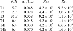
Reference Troldborg, Larsen, Madsen, Hansen, Sørensen and Mikkelsen2011). The effects of the inflow turbulence are negligible on the power and thrust coefficients for the T4l and T4h cases relative to the T4 case. For all other cases, the inflows are generated by precursor simulations with periodic boundary conditions in the horizontal directions. The characteristics of the incoming flow for the different cases are shown in table 2. As seen, the inflow conditions with
 $\unicode[STIX]{x1D6FF}/H$
from 2.7 to 31.7 and
 $u_{\unicode[STIX]{x1D70F}}/U_{hub}$
from 0.028 to 0.058 are significantly different for different cases.
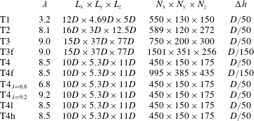
For each simulated turbine, we choose a tip-speed ratio in the optimal wind-power extraction operating regime where power output is maximised. For more description of variable-power wind turbines, see Pao & Johnson (Reference Pao and Johnson2009). The tip-speed ratio, shown in table 3, is chosen according to the wind turbine design and inflow conditions. Two additional cases are created for the T4 turbine, (i)
 $\text{T}4_{\unicode[STIX]{x1D706}=6.8}$
and (ii)
 $\text{T}4_{\unicode[STIX]{x1D706}=9.2}$
, to examine the effects of the tip-speed ratio on the wake meandering characteristics. In these two additional cases, the turbine blade rotational speed is adjusted to maintain a constant tip-speed ratio. The turbine inflow conditions and turbine blade pitch remain the same as in the T4 case.
The characteristics of the incoming wind for the different cases for
 $\unicode[STIX]{x1D6FF}$
, the thickness of the boundary layer,
 $U_{hub}$
, the incoming wind speed at turbine hub height,
 $u_{\unicode[STIX]{x1D70F}}$
, the friction velocity of the incoming turbulent boundary layer,
 $Re_{D}$
, the Reynolds number based on
 $D$
and
 $U_{hub}$
, and
 $Re_{\unicode[STIX]{x1D70F}}$
, the Reynolds number based on
 $\unicode[STIX]{x1D6FF}$
and
 $u_{\unicode[STIX]{x1D70F}}$
.

3.2 Grid resolution study
Using actuator surface models for turbine parametrisation, the grid employed does not have to resolve the boundary layer flow over the blades and nacelle. In the grid resolution study for actuator surface simulations, we do not mean to examine whether the physics near the blade or nacelle is properly resolved or not, but to test whether the mesh is fine enough to capture the wake meandering in turbine far-wake locations. The computational domain, number of grid nodes and grid spacing in the near-turbine region for all cases are listed in table 3. A similar uniform grid spacing (
 $\unicode[STIX]{x0394}h=\unicode[STIX]{x0394}x=\unicode[STIX]{x0394}y=\unicode[STIX]{x0394}z=D/50$
) in the vicinity around the turbine blades is utilised. Outside a
 $2D\times 2D\times 2D$
box around the turbine, stretching is introduced to the grid. Similar grid resolutions have been employed in other studies using actuator-type models (Ivanell et al.
Reference Ivanell, Mikkelsen, Sørensen and Henningson2010; Troldborg et al.
Reference Troldborg, Sorensen and Mikkelsen2010). A grid with resolution similar to the one employed herein has been shown to be sufficient to capture the far-wake dynamics for the T1 turbine in the grid resolution study carried out by Foti et al. (Reference Foti, Yang, Guala and Sotiropoulos2016). However, to ensure that the employed grid resolution is fine enough for utility-scale turbines, several grid resolutions are employed for the T3 and T4 turbine designs to quantify any effects of the grid resolution.
The computational parameters including the tip-speed ratio
 $\unicode[STIX]{x1D706}=\unicode[STIX]{x1D6FA}R/U_{hub}$
(where
 $\unicode[STIX]{x1D6FA}$
is the rotational speed of the rotor,
 $R$
is the radius of the rotor and
 $U_{hub}$
is the incoming wind speed at hub height), the dimensions of the computational domain
 $L_{x}\times L_{y}\times L_{z}$
(where
 $x$
,
 $y$
and
 $z$
denote the downwind, vertical and spanwise directions respectively), the number of grid nodes
 $N_{x}\times N_{y}\times N_{z}$
and the grid spacing
 $\unicode[STIX]{x0394}h=\unicode[STIX]{x0394}x=\unicode[STIX]{x0394}y=\unicode[STIX]{x0394}z$
in the near-turbine region.

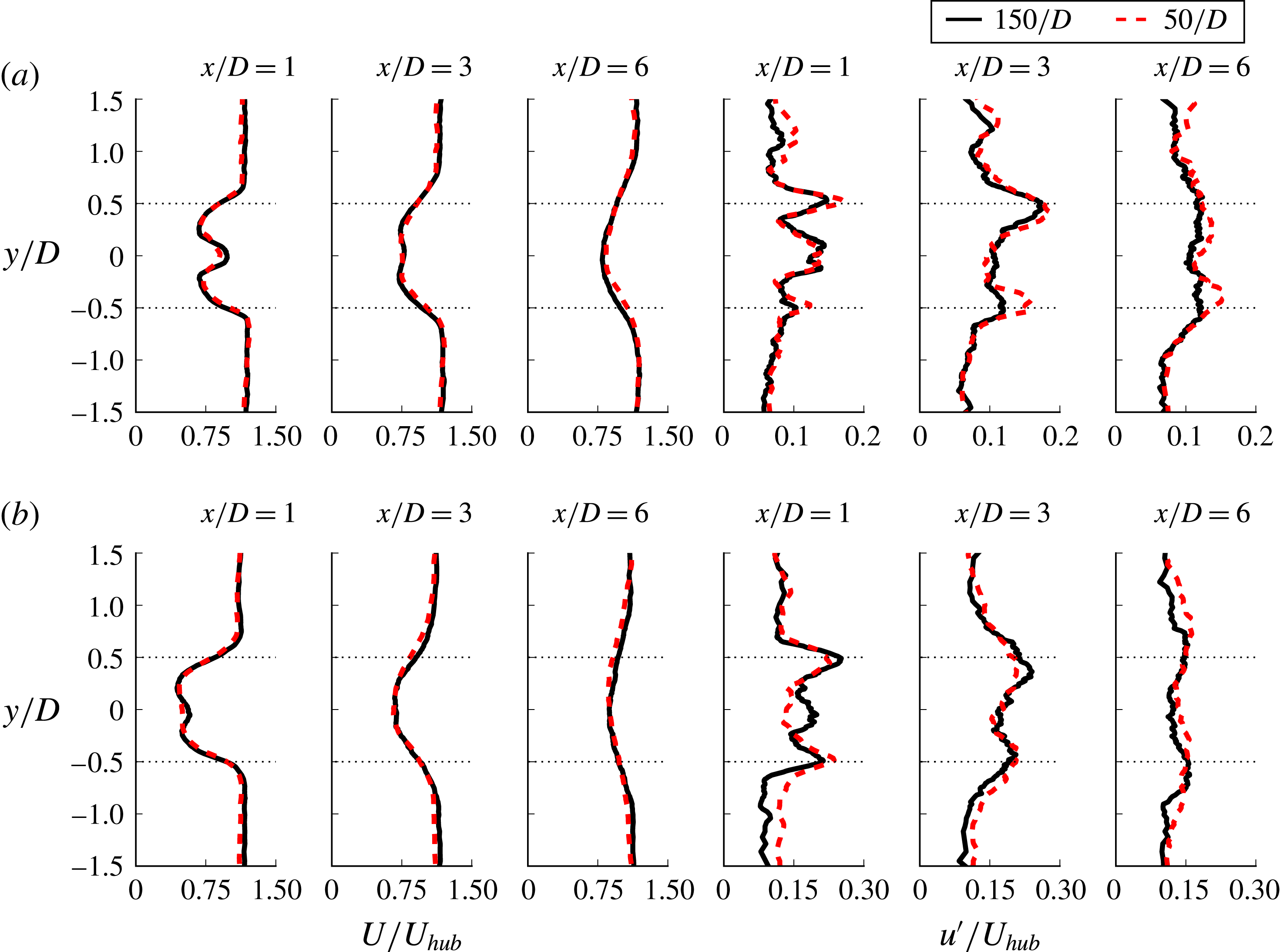
Figure 1 shows a comparison of the mean streamwise velocity
 $U/U_{hub}$
and the streamwise RMS (root-mean-squared) velocity
 $u^{\prime }/U_{hub}$
for the T3 and T4 turbine cases with a near-turbine grid spacing of
 $\unicode[STIX]{x0394}h=D/50$
, and the T3f and T4f turbine cases with a near-turbine grid spacing of
 $\unicode[STIX]{x0394}h=D/150$
. The spanwise profiles of the mean streamwise velocity shown at the
 $x/D=1,3$
and 6 turbine downwind locations compare well between the fine and coarse grid resolutions for each respective turbine design. There is less than a 5 % difference at any location, ensuring that the actuator surface model with nacelle is able to accurately predict the mean velocity using a coarse grid resolution. The streamwise RMS velocity also has a favourable comparison between the respective coarse and fine resolutions. A slightly higher difference throughout the profiles occurs due to the different grid resolutions; however, the overall shapes of the profiles with the peaks near the turbine blade tip locations are consistent.
Comparison of the grid resolutions of (a) T4, T4f and (b) T3, T3f with the spanwise profiles of the mean streamwise velocity
 $U$
and streamwise RMS velocity
 $u^{\prime }$
non-dimensionalised by the incoming hub height velocity
 $U_{hub}$
. The horizontal dotted lines at
 $z/D=\pm 0.5$
are the tip positions.

3.3 Method validation
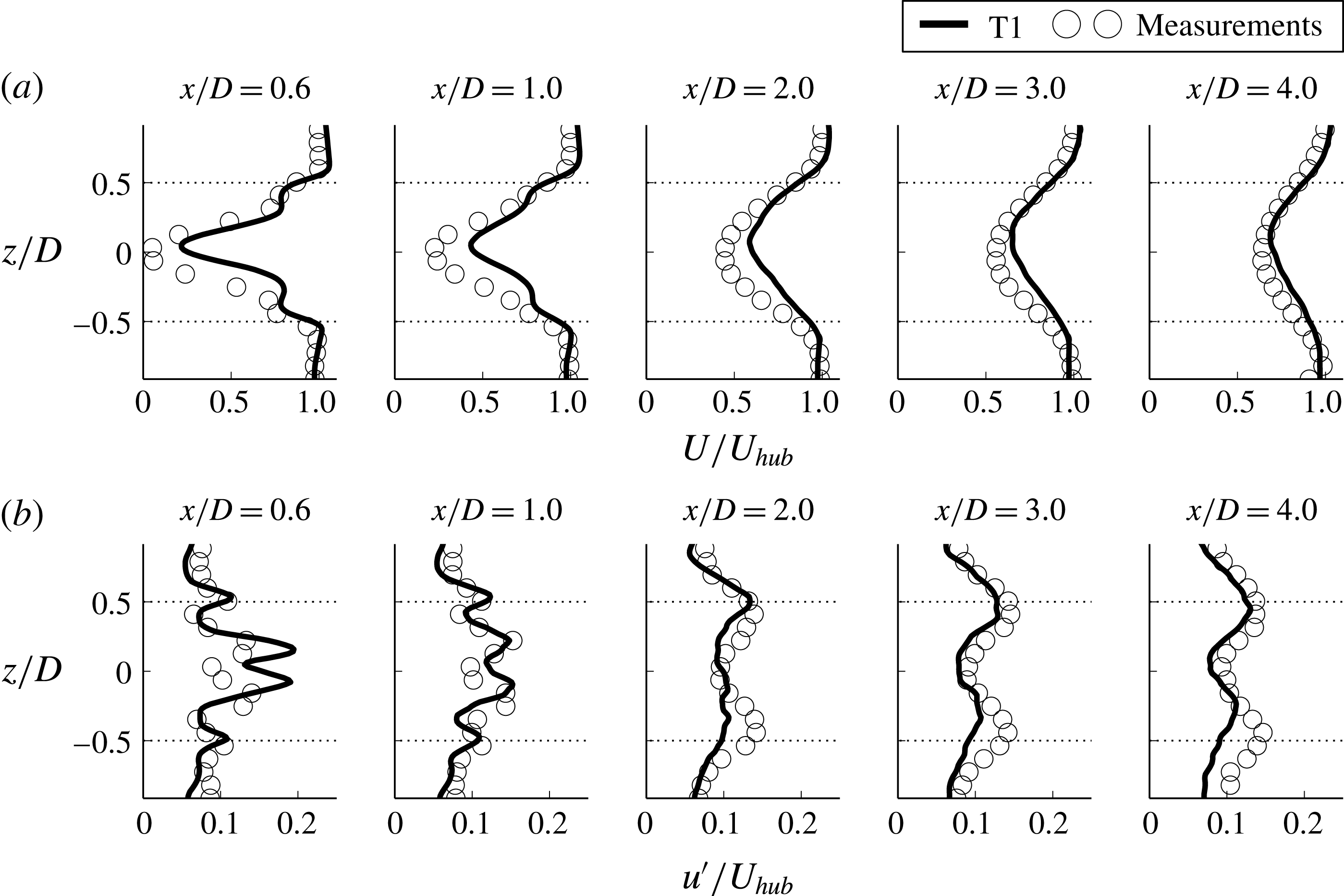
Experimental measurements from the T1 and T2 turbines are available to validate the numerical methods used for the simulations. First, the computed results for the T1 turbine case are compared with measurements. Several spanwise profiles of the mean streamwise velocity
 $U$
, non-dimensionalised by the hub velocity
 $U_{hub}$
, of the simulation and the experimental particle image velocimetry (PIV) measurements (Howard et al.
Reference Howard, Singh, Sotiropoulos and Guala2015b
) are shown in figure 2(a). The simulation is able to accurately capture the mean wake recovery from
 $x/D=0.6$
to far downwind. At
 $x/D=0.6$
downwind of the turbine, the simulation, capturing 90 % of the velocity deficit at the centreline, reproduces the large wake deficit caused by the nacelle and the separate wake structure caused by the blades. The former wake structure is referred to as the inner wake while the latter is the outer wake. The nacelle model creates the necessary deficit at the centreline, and the actuator surface model for the blades is able to capture the outer wake with good agreement despite the coarse grid resolution used in comparison to the immersed boundary simulation described by Foti et al. (Reference Foti, Yang, Guala and Sotiropoulos2016). The centreline behaviour converges to the mean velocity measurements by
 $x/D=3$
. As discussed by Foti et al. (Reference Foti, Yang, Guala and Sotiropoulos2016), there is a flow reversal region directly behind the turbine with a stagnation point along the centreline at
 $x/D=0.4$
where the inner wake starts to rapidly recover. As we progress to
 $x/D=1$
, the inner wake recovers quickly, while the separate structures near
 $z/D\pm 0.5$
merge into the wake. By
 $x/D=2$
, there is no distinction between the inner and outer wake. The wake slowly recovers as the distance from the turbine increases. The comparisons of the measurements and the simulations of the streamwise RMS velocity
 $u^{\prime }$
non-dimensionalised by the hub velocity
 $U_{hub}$
are shown in figure 2(b). At
 $x/D=0.6$
, the
 $u^{\prime }$
of the simulation results clearly shows the peaks representing the two shear layers in the wake: the outer shear layer at
 $z/D\pm 0.5$
between the ambient flow and the outer wake, and the inner shear layer
 $z/D=\pm 0.1$
between the wake behind the nacelle and the outer wake. The RMS velocity compares well with the measurements.
Comparisons of the spanwise profiles of the T1 simulation and measurements from Howard et al. (Reference Howard, Singh, Sotiropoulos and Guala2015b
) (symbols) of mean flow quantities non-dimensionalised by the incoming hub height velocity
 $U_{hub}$
. (a) Streamwise velocity
 $U$
; (b) streamwise velocity fluctuation
 $u^{\prime }$
. The horizontal dotted lines at
 $z/D=\pm 0.5$
are the tip positions.

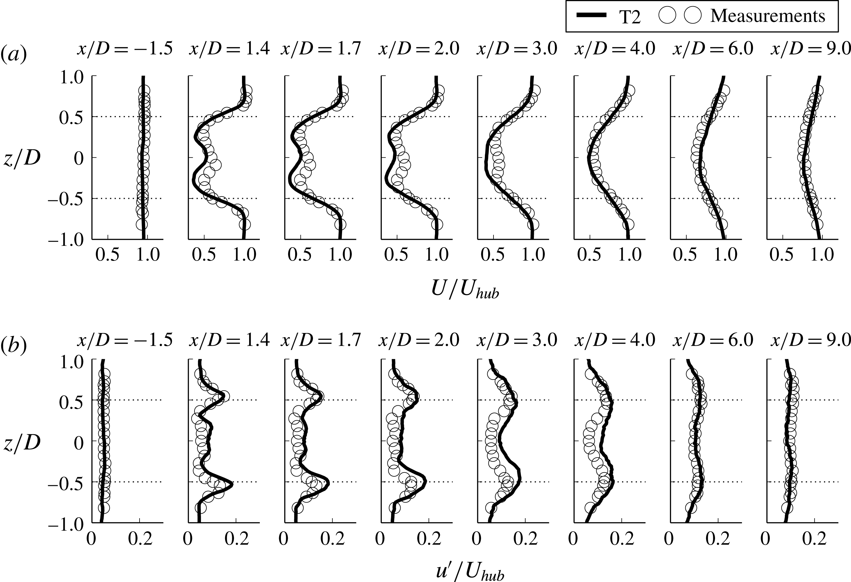
Further validation is shown for the T2 turbine in figure 3. We compare the experimental measurements taken through a hot wire probe for the G1 model turbine (Foti et al.
Reference Foti, Yang, Campagnolo, Maniaci and Sotiropolos2018) with the present T2 simulation. Figure 3(a) shows the mean streamwise velocity profiles of both the measurements and the simulation. In the first profile behind the turbine,
 $x/D=1.4$
, the fine details of the separate inner and outer wake have already been smeared out by the turbulence. The effect of the nacelle on the wake is the creation of a large flat region that appears in the centreline which is captured by all simulations. Farther downwind, the wake recovery is accurately captured and the profiles converge to the measurements. The simulation is able to readily reproduce the turbulence, the streamwise RMS velocity
 $u^{\prime }$
and the inner wake shear layer near the turbine, as shown in figure 3(b). Farther downwind, the profiles converge to the measurements. From both validation studies, we conclude that the simulations are able to predict the wake characteristics of wind turbines well.
Comparisons of the spanwise profiles of the T2 simulation and measurements from Foti et al. (Reference Foti, Yang, Campagnolo, Maniaci and Sotiropolos2018) (symbols) of mean flow quantities non-dimensionalised by the incoming velocity at the turbine hub height
 $U_{hub}$
. (a) Streamwise velocity
 $U$
; (b) streamwise velocity fluctuation
 $u^{\prime }$
. The horizontal dotted lines at
 $z/D=\pm 0.5$
are the tip positions.

4 Results
In what follows, we present and analyse the computed results for the four turbines. We show the time-averaged wake characteristics in § 4.1 and the analysis of wake meandering in § 4.2.
4.1 Time-averaged wake characteristics
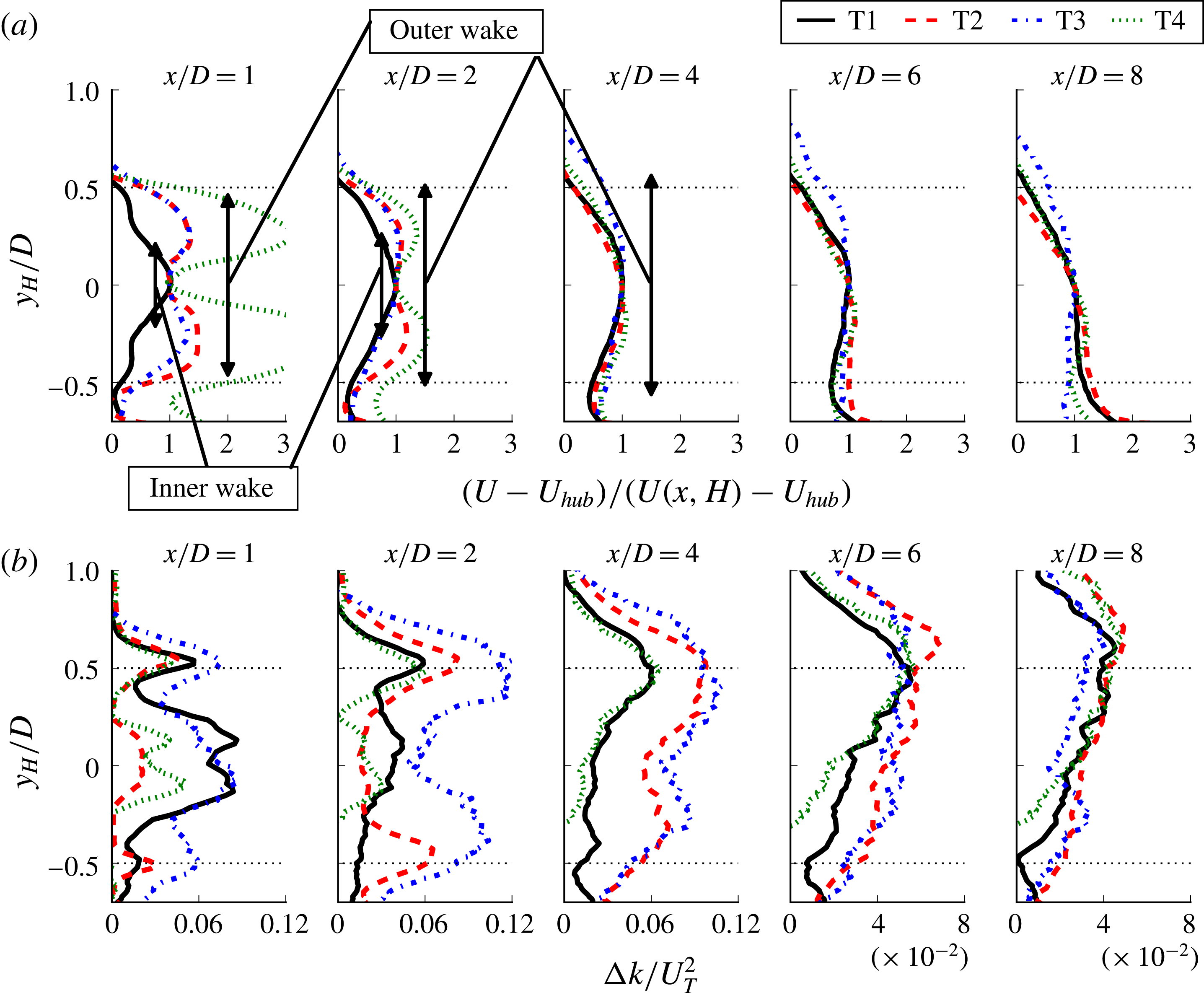
In this section, we study the effects of turbine rotor scale on the time-averaged flow field behind the turbines. First, we show the mean downwind velocity deficit profiles in figure 4(a). In order to show the profiles of different sized turbines clearly, the origin of the vertical coordinate normalised by the rotor diameter is translated to the turbine hub height,
 $H$
, such that
 $y_{H}=y-H$
. As can be seen, all of the turbine wakes at
 $x/D=1$
close to the turbine exhibit two distinct wake regions: the inner wake mainly formed by the nacelle and the outer wake created by the blades. However, the relative strength of the inner wake to the outer wake is significantly different for different turbines. The velocity deficit in the inner wake of turbine T1 is significantly higher than that in the outer wake. The velocity deficits in the inner wakes of the other three turbines, on the other hand, are smaller than those in the outer wakes formed by the blades. At downwind locations
 $x/D=2$
and
 $4$
, as shown in figure 4(a), the inner wakes for all turbines begin to merge with the respective outer wakes, with substantial decreases in the velocity deficits. By locations
 $x/D=6$
and
 $8$
, the profiles of each turbine begin to collapse together, showing that the mean velocity deficit at hub height is a proper scale for the mean velocity deficit profiles in the far wake for the present turbine designs and operating conditions. We expect that velocity profiles will continue to approach a similar profile at further downstream locations.
The turbine-added turbulence kinetic energy (TKE),
 $\unicode[STIX]{x0394}k/U_{T}^{2}$
, is shown in figure 4(b), where
 $U_{T}$
is the characteristic velocity, defined as follows:
 $$\begin{eqnarray}U_{T}=\left(T/\unicode[STIX]{x1D70C}\unicode[STIX]{x03C0}R^{2}\right)^{1/2},\end{eqnarray}$$
where
 $T$
is the thrust on the turbine,
 $\unicode[STIX]{x1D70C}$
is the air density and
 $R$
is the rotor radius. The turbine-added TKE is calculated by subtracting the inflow TKE from the TKE in the wake. It was shown by Yang et al. (Reference Yang, Howard, Guala and Sotiropoulos2015a
) that
 $U_{T}$
can properly scale the turbine-added TKE at far-wake locations for different inflow conditions. The characteristic velocity scale provides an association with the turbine-added TKE and the initial velocity deficit imposed on the wake by the thrust. Close to the turbine at
 $x/D=1$
, the effects of the nacelle and the blades on the flow field are evident by the existence of peaks of turbine-added TKE along the tip positions and the inner wake shear layer. All simulations show similar features. At locations
 $x/D=2$
and
 $4$
, the peak TKE along the top-tip position increases compared with the near-turbine position
 $x/D=1$
. The levels of the turbine-added TKE in the inner wake diminish rapidly as the shear layer of the inner wake spreads and merges with the outer wake. This behaviour has also been observed in several other studies, including Kang et al. (Reference Kang, Yang and Sotiropoulos2014) and Foti et al. (Reference Foti, Yang, Guala and Sotiropoulos2016), and is linked to the onset of wake meandering. At
 $x/D=6$
and
 $8$
, the characteristic velocity
 $U_{T}$
begins to properly scale and collapse the profiles of the turbine-added TKE, suggesting that turbine thrust and TKE caused by wake meandering are strongly correlated. The turbine-added TKE in the wake is primarily due to the process of mean energy extraction from the incoming flow which increases the production of TKE. This mean energy extraction and turbulence energy addition is represented in the characteristic velocity defined. The scaling begins mainly near the turbine top-tip location (
 $y/y_{H}=0.5$
) where the maximum amount of energy is injected into the wake. By
 $x/D=8$
, the region of profile convergence grows to encompass the majority of the wake.
Comparisons of vertical profiles of the (a) mean downwind velocity
 $(U-U_{hub})/(U(x,H)-U_{hub})$
and (b) turbine-added TKE
 $\unicode[STIX]{x0394}k/U_{T}^{2}$
for each turbine design simulation at several turbine downwind locations where the vertical coordinate is
 $y_{H}=y-H$
. The inner wake and outer wake regions are delineated in (a).

4.2 Wake meandering statistics
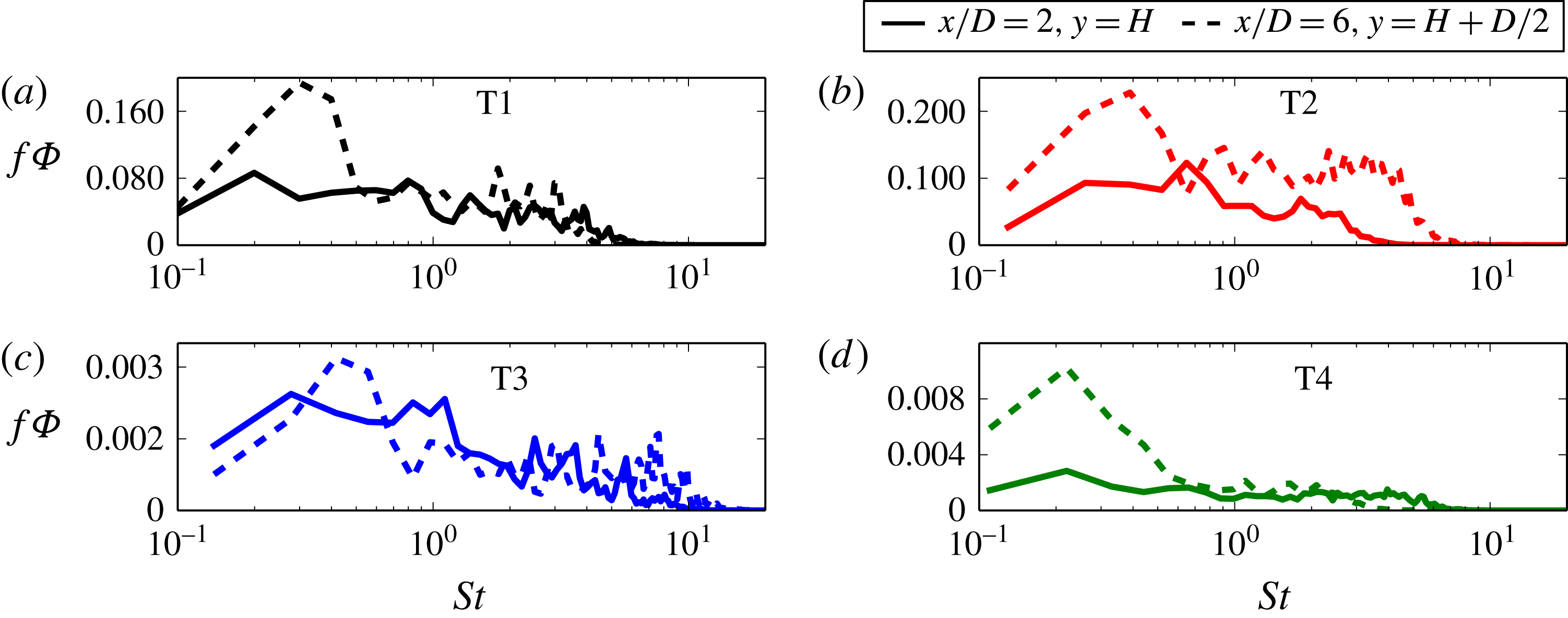
We begin our discussion of wake meandering dynamics by considering the spectral signature of wake meandering for each turbine to investigate the occurrence of common Strouhal numbers for different turbine designs, as shown in figure 5. The Fourier power spectral density
 $\unicode[STIX]{x1D6F7}$
of the streamwise component of the velocity fluctuations premultiplied by the frequency
 $f$
at
 $x/D=2$
reveals a range of common frequencies around
 $St=0.7{-}0.8$
, which is consistent with the hub vortex frequency (Iungo et al.
Reference Iungo, Viola, Camarri, Porté-Agel and Gallaire2013; Howard et al.
Reference Howard, Singh, Sotiropoulos and Guala2015b
; Foti et al.
Reference Foti, Yang, Guala and Sotiropoulos2016). The power spectral densities for all turbines at
 $x/D=6$
reveal the existence of a lower frequency of
 $St=0.25$
–
 $0.3$
which occurs only in the far wake. Corroborating observations of a low-frequency mode have been reported in a variety of wind turbine studies:
 $St=0.23$
(Okulov & Sørensen Reference Okulov and Sørensen2007),
 $St=0.28$
(Chamorro et al.
Reference Chamorro, Hill, Morton, Ellis, Arndt and Sotiropoulos2013),
 $St=0.15$
(Foti et al.
Reference Foti, Yang, Guala and Sotiropoulos2016) and
 $St=0.15{-}0.25$
(Medici & Alfredsson Reference Medici and Alfredsson2008). Okulov et al. (Reference Okulov, Naumov, Mikkelsen, Kabardin and Sørensen2014) reported a similar Strouhal number for turbines at different operating conditions. A major contribution of our work is to conclusively show that a similar near- and far-wake meandering Strouhal number for different turbine designs exists across a broad range of turbine rotor sizes, which suggests that a regular frequency of the hub vortex and wake meandering dominate turbine wakes regardless of the turbine size and turbine design.
The Fourier power spectral density of the streamwise component of the velocity fluctuations premultiplied by the frequency,
 $f\unicode[STIX]{x1D6F7}$
, for each turbine design simulation.

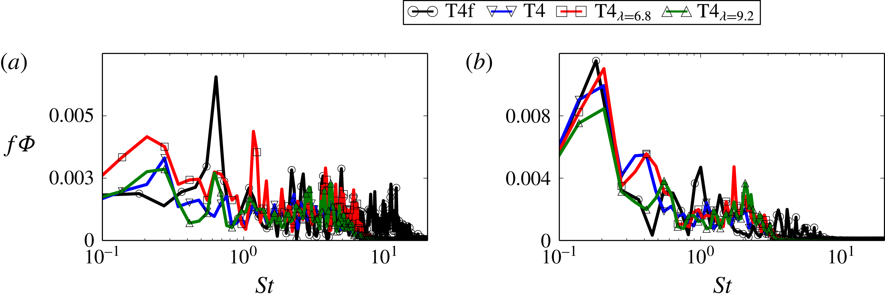
Further evidence of common Strouhal numbers for the hub vortex and wake meandering is shown in figure 6 for several T4 turbine design cases with three different tip-speed ratios, as shown in table 3. At
 $x/D=2,y=H$
, the hub vortex frequency mode is not well distinguished except in the fine grid resolution case, T4f, where a large spectral signature is prominent around
 $St=0.7$
. The other three cases with the coarser grid resolution of
 $\unicode[STIX]{x0394}h=D/50$
do not have an energy mode with similar magnitude. The differences can be attributed to the grid resolution in the near wake. On the other hand, the wake meander frequency mode is readily seen for each case in figure 6(b) at
 $x/D=6$
,
 $y=H+D/2$
, with a similar energy density regardless of tip-speed ratio or grid resolution. This provides the evidence that the wake meandering Strouhal number is invariant across this range of tip-speed ratios.
The Fourier power spectral density of the streamwise component of the velocity fluctuations premultiplied by frequency,
 $f\unicode[STIX]{x1D6F7}$
, for T4, T4f,
 $\text{T}4_{\unicode[STIX]{x1D706}=6.8}$
and
 $\text{T}4_{\unicode[STIX]{x1D706}=9.2}$
at (a)
 $x/D=2,y=H$
and (b)
 $x/D=6,y=H+D/2$
.

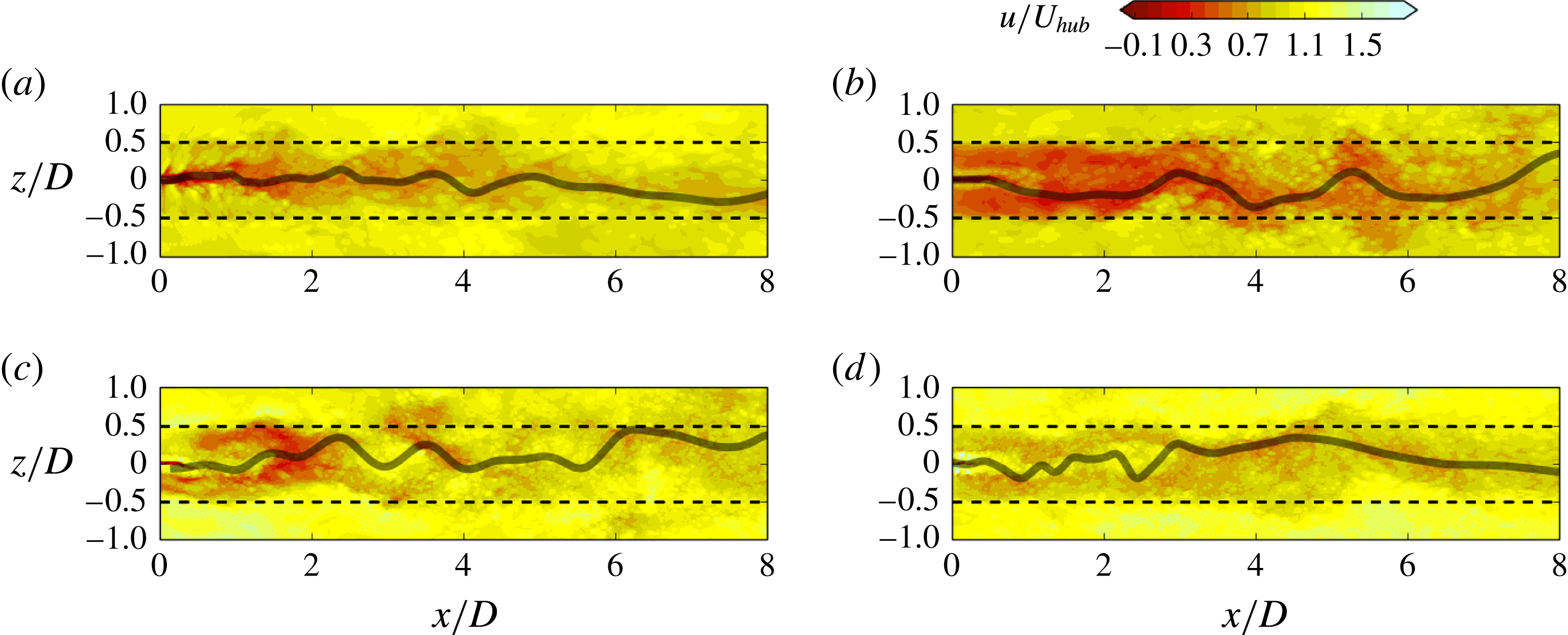
Instantaneous downwind velocity contours with a meander profile (line) at the hub height plane for simulations of (a) T1, (b) T2, (c) T3 and (d) T4.

We now focus on the dynamics and statistics of wake meandering using the filtering technique developed by Foti et al. (Reference Foti, Yang, Guala and Sotiropoulos2016) for tracking the velocity minimum at each downwind location. This technique was developed based on the work of Howard et al. (Reference Howard, Singh, Sotiropoulos and Guala2015b
). A temporally and spatially evolving flow field
 $\boldsymbol{u}(\boldsymbol{x},t)$
(bold indicates a vector quantity) can be decomposed into three parts as follows:
 $$\begin{eqnarray}\boldsymbol{u}(\boldsymbol{x},t)=\boldsymbol{U}(\boldsymbol{x})+\tilde{\boldsymbol{u}}(\boldsymbol{x},t)+\boldsymbol{u}_{i}(\boldsymbol{x},t),\end{eqnarray}$$
where
 $\boldsymbol{U}(\boldsymbol{x})$
is the mean strictly spatial term,
 $\tilde{\boldsymbol{u}}(\boldsymbol{x},t)$
is the coherent term and
 $\boldsymbol{u}_{i}(\boldsymbol{x},t)$
is the incoherent term. In the technique of Foti et al. (Reference Foti, Yang, Guala and Sotiropoulos2016), a temporal filtering process proposed by Chrisohoides & Sotiropoulos (Reference Chrisohoides and Sotiropoulos2003) is applied to filter out the incoherent term in (4.2). The coherent time scale
 $\unicode[STIX]{x1D70F}_{c}$
employed in the temporal filtering process is related to the turbine rotational period
 $T$
and equals
 $0.6T$
, which is found using fluctuation analysis and the central limit theorem (Chrisohoides & Sotiropoulos Reference Chrisohoides and Sotiropoulos2003). The velocity minimum is then found from the temporally filtered velocity field
 $U(x)+\tilde{u} (x,t)$
. The meander profile is constructed using a low-pass spatial filter with a length scale
 $l_{c}=D/2$
on the velocity minima. The amplitude
 $A$
and wavelength
 $\unicode[STIX]{x1D706}$
characterising the wake meandering are finally extracted from the wave-like velocity minimum profiles.
Figure 7(a–d) shows the meander profile overlaid on the contours of instantaneous downwind velocity
 $u/U_{hub}$
for each simulation. As already shown in figure 4, the flow fields at near-wake locations are significantly different for each turbine: the inner wake of the T1 turbine has a single recirculation zone while the inner wakes of the other three turbines, on the other hand, consist of a slow positive-velocity region behind the nacelle surrounded by high-velocity root vortices. For all of the turbines, the meander profiles successfully track the slow inner wake at near-wake locations. As the inner wake recovers and merges with the outer wake at around
 $2D$
downwind of the turbine location, large-scale wake meandering starts for all of the four turbines. At further downwind locations, the amplitude and wavelength increase for all four turbines. At downwind locations starting around
 $x/D=4$
, the wavelength and amplitude of the meander profiles seem to be qualitatively similar for each turbine.
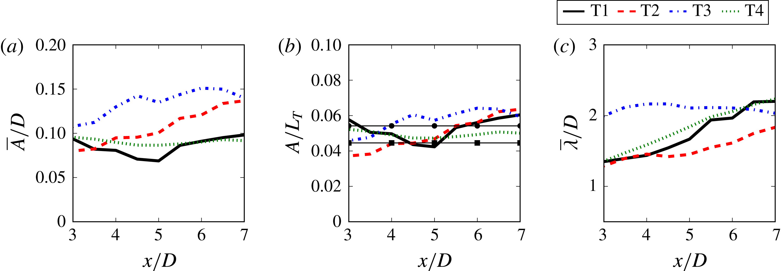
Mean amplitudes and wavelengths of meander profiles for different turbine designs. (a) Amplitude scaled by rotor diameter,
 $\overline{A}/D$
; (b) amplitude scaled by the characteristic length
 $L_{T}$
,
 $\overline{A}/L_{T}$
, with squares for results by Davies (Reference Davies1976) and circles for results by Bisset, Antonia & Browne (Reference Bisset, Antonia and Browne1990) for the meandering amplitudes of bluff bodies (the length scale
 $L_{T}$
for the stationary bluff bodies is based on the drag rather than the thrust); (c) wavelength scaled by diameter,
 $\overline{\unicode[STIX]{x1D706}}/D$
.

In order to quantitatively determine the amplitudes and wavelengths of the wake meanders for each turbine simulation, the three-dimensional meander profiles are projected onto the two-dimensional hub height plane to obtain a wave-like profile (e.g. the profiles shown in figure 7) with deterministic amplitudes and wavelengths. The amplitudes of a meander profile are determined by the distance from the centre of the wave-like meander profile to the spanwise extremum. Similarly, the wavelengths of the meander profile are captured by calculating the distance between successive maxima or minima. The examples of the meander profiles for each simulation provided in figure 7 readily show that each meander profile contains a distribution of amplitudes and wavelengths with respect to the downwind distance. The means of the quantities characterising the wave-like meandering motion with respect to the downwind distance are calculated by collecting all of the amplitudes and wavelengths of all meandering profiles for each simulation into half-diameter bins. Figure 8(a) shows the mean amplitude
 $\overline{A}$
scaled by the rotor diameter
 $D$
for each simulation, which indicates that generally the amplitude increases with the downwind distance and is proportional to the diameter of the turbine. However, the values of
 $\overline{A}/D$
are quite different for each turbine, especially at far-wake locations. We propose a new reference length to scale meandering amplitudes, which is defined as follows:
 $$\begin{eqnarray}L_{T}=U_{T}/f_{m},\end{eqnarray}$$
where
 $f_{m}$
is the frequency derived from the dominant Strouhal number
 $St_{m}$
of wake meandering in the spectral analysis presented in figure 5. As shown in figure 8(b), the amplitude is properly scaled when normalised by the length scale
 $L_{T}$
. The near collapse of the amplitude profiles suggests that the wake meandering amplitude is strongly correlated with the velocity scale of the turbine-added TKE and the time scale of the wake meandering. Since the thrust force on the rotor
 $T=(1/2)\unicode[STIX]{x1D70C}C_{T}\unicode[STIX]{x03C0}R^{2}U_{hub}^{2}$
depends on the thrust coefficient
 $C_{T}$
, the collapse in figure 8(b) indicates the possibility of controlling the meandering amplitude through different rotor designs and turbine control algorithms. The wake meandering amplitudes of different turbine designs are compared with the computed spanwise displacements of the centres of vortices in the wake of a circular cylinder (Bisset et al.
Reference Bisset, Antonia and Browne1990) and a D-shaped cylinder (Davies Reference Davies1976). In Davies (Reference Davies1976) and Bisset et al. (Reference Bisset, Antonia and Browne1990), the vortex spanwise displacements are obtained using conditional averaging techniques similar to the interval averaging technique we employ herein to calculate the meander profiles. A single displacement far downstream from the bluff body was reported in each reference. This single value is used across the domain in figure 8(b). Our implicit assumption that the spanwise displacement of vortices shed in the wake of bluff bodies is analogous to the meander amplitude in wind turbines is supported by Howard et al. (Reference Howard, Singh, Sotiropoulos and Guala2015b
), who showed that vortices in the wake of wind turbines modulate the meander profile. The length scale
 $L_{T}$
for the stationary bluff bodies is based on the drag rather than the thrust. The fact that the meandering amplitudes of wind turbine wakes are similar to these more simplistic bluff bodies suggests that the effect of the turbine rotor on the wake meandering dynamics at far-wake locations can be well represented by a bluff body with a single parameter,
 $L_{T}$
. On the other hand, the mean wavelength of the meander profiles is directly related to the turbine size and, in fact, is properly scaled by the diameter. As shown in figure 8(c), the mean wavelength grows from nearly the size of the diameter to twice the diameter in the downwind distance range of
 $3\leqslant x/D\leqslant 7$
. Contrary to the relationship of the amplitudes to the turbine-added turbulence, the wavelengths are related to the velocity deficit, which stretches the wake meanders as the velocity recovers.
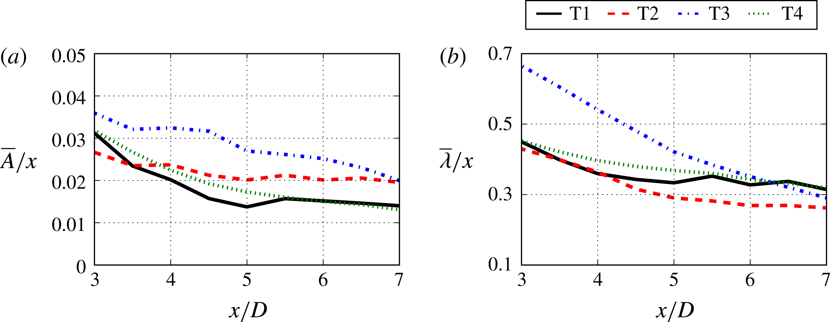
Mean amplitudes and wavelengths of meander profiles for different turbine designs. (a) Amplitude scaled by downwind distance and (b) wavelength scaled by downwind distance.

Use of
 $L_{T}$
as a characteristic length scale does not take into account the streamwise variations of the meandering amplitude and wavelength. The wake radius is usually assumed to grow linearly in low-fidelity kinematic models (Jensen Reference Jensen1983; Frandsen Reference Frandsen1992; Yang et al.
Reference Yang, Kang and Sotiropoulos2012). To test this linear growth assumption in wake meandering, we show in figure 9 the variations in the meandering amplitude and wavelength normalised by the downwind distance from the turbine
 $x$
for the four turbine designs. First, we see that at
 $x/D>5.5$
, the profiles are fairly constant for the T1, T2 and T4 cases, which suggests that linear growth of the meandering amplitude and wavelength is a reasonable assumption. However, this scaling does not perform as well for the T3 turbine design. It is also seen that the variances of
 $A$
and
 $\unicode[STIX]{x1D706}$
when normalised by the downwind distance without taking into account different growth rates are similar to those normalised by
 $D$
, as expected. Reduction of these variances requires case-specific growth rates, which depend on many factors, such as turbine operational conditions and incoming turbulence, and can hardly be simply formulated. The
 $L_{T}$
scale, on the other hand, only requires the thrust coefficient and the incoming wind speed at turbine hub height, which are usually available for turbines in wind farms. In terms of developing low-fidelity models for utility-scale wind farms, we believe that
 $L_{T}$
is a more effective scaling for
 $A$
compared with the complexities that might appear in a downwind-dependent scaling. Furthermore, if we substitute (4.1) into (4.3), an interesting expression for the characteristic length scale
 $L_{T}$
can be obtained, which relates the thrust coefficient, rotor diameter and dominant wake meandering Strouhal number
 $St_{m}$
as follows:
 $L_{T}=(\sqrt{2}/2)(\sqrt{C_{T}}/St_{m})D$
. The quantities on the right-hand side of this expression can all be determined a priori without having to obtain the velocity fields in the wake. This observation is consistent with that in the wind tunnel experiment of Medici & Alfredsson (Reference Medici and Alfredsson2008), who reported a similar wake meandering
 $St$
and showed the influence of thrust on wake meandering.
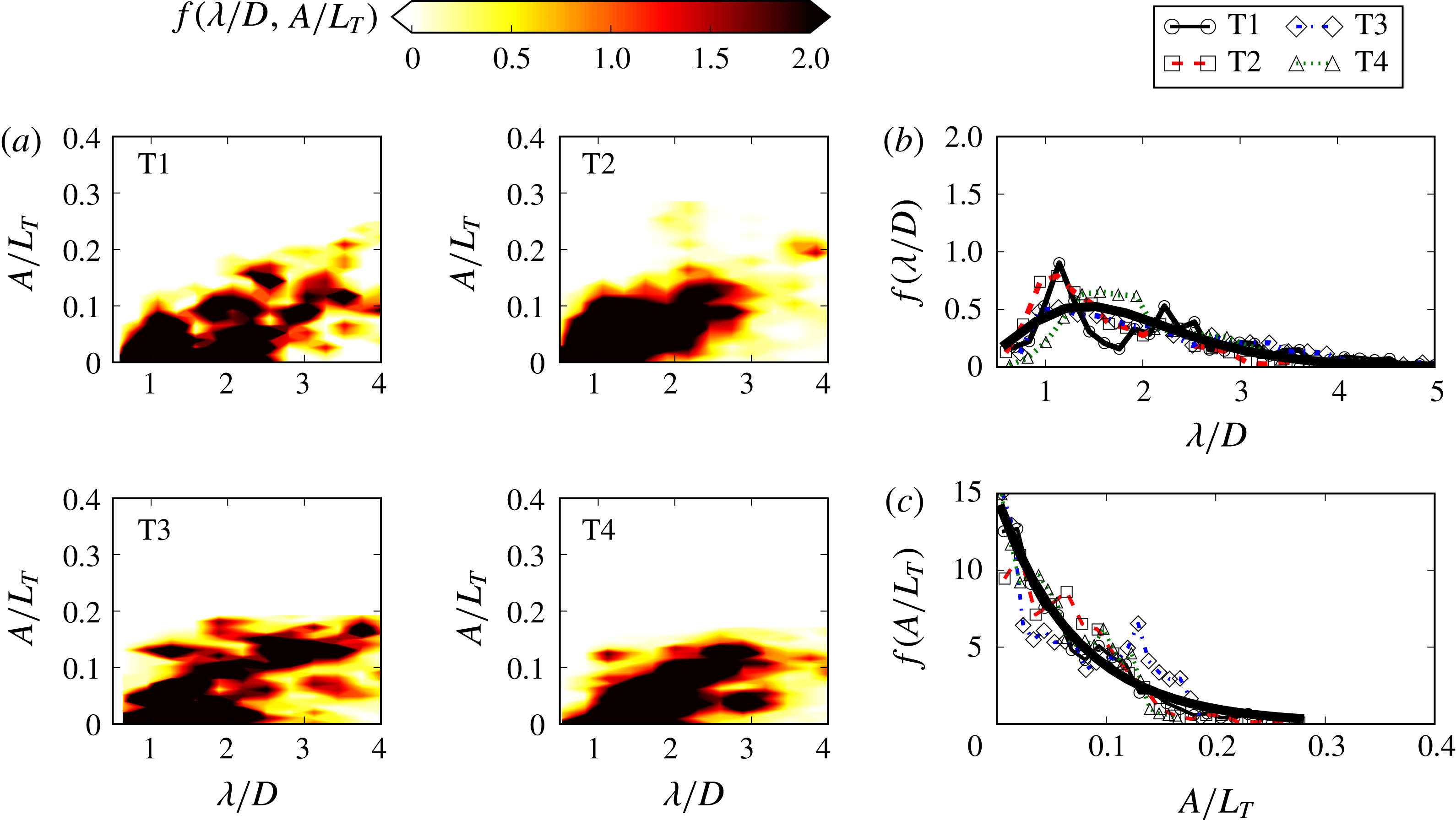
Meander profile statistics: (a) contours of JPDF
 $f(A/L_{T},\unicode[STIX]{x1D706}/D)$
for the simulations; (b) PDF of wavelength
 $f(\unicode[STIX]{x1D706}/D)$
with curve-fitted gamma distribution
 $\unicode[STIX]{x1D6E4}(\unicode[STIX]{x1D6FC}=4.0,\unicode[STIX]{x1D6FD}=2.2)$
(solid line); (c) PDF of amplitude
 $f(A/L_{T})$
with curve-fitted gamma distribution
 $\unicode[STIX]{x1D6E4}(\unicode[STIX]{x1D6FC}=1.0,\unicode[STIX]{x1D6FD}=2.62)$
(solid line) for the simulations at
 $x/D=6$
. The gamma distribution
 $\unicode[STIX]{x1D6E4}(\unicode[STIX]{x1D6FC},\unicode[STIX]{x1D6FD})$
is given by
 $\unicode[STIX]{x1D6E4}(\unicode[STIX]{x1D6FC},\unicode[STIX]{x1D6FD})=f(x;\unicode[STIX]{x1D6FC},\unicode[STIX]{x1D6FD})=(\unicode[STIX]{x1D6FD}^{\unicode[STIX]{x1D6FC}}/\unicode[STIX]{x1D6E4}(\unicode[STIX]{x1D6FC}))x^{\unicode[STIX]{x1D6FC}-1}\,\text{e}^{\unicode[STIX]{x1D6FD}x}$
, where
 $\unicode[STIX]{x1D6FC}$
is the shape parameter and
 $\unicode[STIX]{x1D6FD}$
is the rate parameter.

The statistics of wake meandering amplitudes and wavelengths are further investigated by the joint probability density function (JPDF) for each simulation in figure 10(a). The JPDFs are created by binning corresponding scaled amplitudes
 $A/L_{T}$
and wavelengths
 $\unicode[STIX]{x1D706}/D$
over a one-diameter-long interval centred at
 $x/D=6$
. The JPDF of the T1 turbine is maximum around
 $A/L_{T}=0.05$
and
 $\unicode[STIX]{x1D706}/D=1$
, with regions of high probability extending to
 $A/L_{T}=0.1$
and
 $\unicode[STIX]{x1D706}/D=1$
and
 $A/L_{T}=0.15$
and
 $\unicode[STIX]{x1D706}/D=2$
. The region of
 $A/L_{T}>2$
and
 $\unicode[STIX]{x1D706}/D>3$
is marked by relatively high probability, indicating that wavelengths much longer than the diameter exist, but only in conjunction with larger amplitudes. The JPDF of the larger T2 turbine exhibits regions of high probability similar to the T1 turbine. Both turbines have high probability extending to regions with
 $\unicode[STIX]{x1D706}/D=1$
and
 $2$
with amplitude
 $A/L_{T}=0.1$
. The JPDF includes the high-probability regions of large amplitude and wavelength. The JPDF of the T3 turbine also shows a region of high probability like the two previous smaller turbines. However, there are also regions of higher amplitude and low wavelength and low amplitude and high wavelength that are not found in the other turbines. The T4 turbine shows a JPDF that is similar to the other three, with a similar shape of the region of highest probability between
 $A/L_{T}\leqslant 0.15$
and
 $1\leqslant \unicode[STIX]{x1D706}/D\leqslant 2$
. There is a slight shift towards higher wavelengths, which corresponds with the slightly higher shifted
 $f(St^{m})$
in figure 5(d). Interestingly, the observations of the amplitude–wavelength JPDFs for each turbine simulation are remarkably similar, and the rotor diameter has little influence on the probability when the amplitude and wavelength are properly scaled. A final assessment of the amplitude and wavelength probability density functions (PDFs) is shown in figure 10(b,c). A univariate PDF is created for each turbine simulation at
 $x/D=6$
. The PDFs are similar for each turbine, and the PDFs can be modelled using a gamma distribution
 $\unicode[STIX]{x1D6E4}(\unicode[STIX]{x1D6FC},\unicode[STIX]{x1D6FD})$
.
Mean amplitudes and wavelengths of meander profiles for different T4 turbine cases. (a) Amplitude scaled by characteristic length
 $L_{T}$
,
 $\overline{A}/L_{T}$
; (b) wavelength scaled by diameter,
 $\overline{\unicode[STIX]{x1D706}}/D$
, at
 $x/D=6$
; (c) PDF of amplitude
 $f(A/L_{T})$
; (d) PDF of wavelength
 $f(\unicode[STIX]{x1D706}/D)$
, at
 $x/D=6$
.

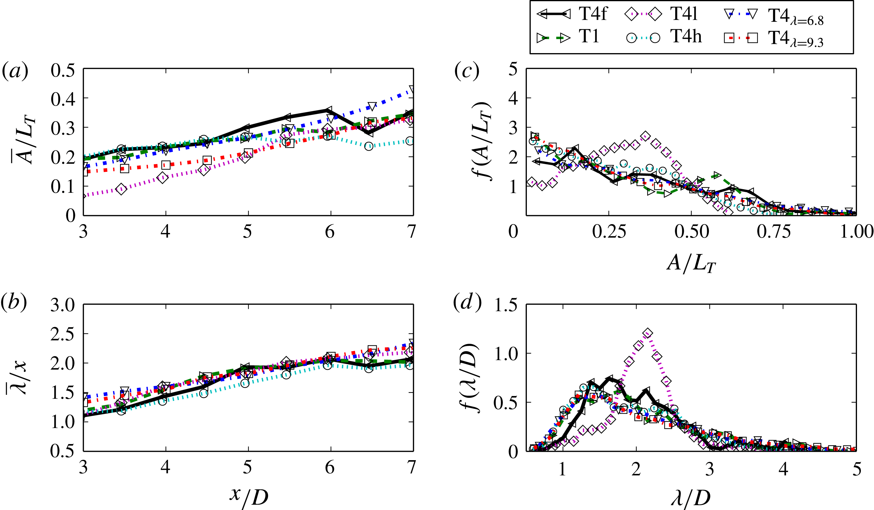
Further observations on the scaling behaviour of the meander profile statistics are evident by focusing on the different operating conditions of the T4 turbine. Figure 11(a) shows the average amplitude scaled by
 $L_{T}$
for each T4 operating case. First, both the finer grid T4f and coarser T4 cases have a similar average amplitude, indicating that the grid resolution of
 $\unicode[STIX]{x0394}h=50$
is sufficient for resolving the meander statistics. Another behaviour of wake meandering demonstrated with the different tip-speed ratio cases is that the blade rotational speed has little effect on the meandering amplitude. This result shows that
 $L_{T}$
properly scales the meander amplitude regardless of the tip-speed ratio. Finally, the incoming turbulence intensity has an effect on the wake meandering amplitude in such a way that lower incoming turbulence induces wake meandering further downwind. However, at
 $x/D=5.5$
for T4l, the meandering amplitude increases to the same magnitude as the other cases. The average scaled wavelength
 $\unicode[STIX]{x1D706}/D$
is shown in figure 11(b). All T4 cases maintain the same wavelength throughout the wake. This further indicates that the wavelength is decoupled from the operating conditions. Profiles of the PDF of the amplitude
 $f(A/L_{T})$
and the wavelength
 $f(\unicode[STIX]{x1D706}/D)$
at
 $x/D=6$
are shown in figure 11(c) and figure 11(d) respectively. Except for the low-turbulence-intensity inflow case T4l, the PDFs of the wavelengths and amplitudes have similar profiles for different cases. The low-turbulence-intensity inflow has an effect on the variance of both the scaled wavelength and to a lesser effect the scaled amplitude. While the average scaled wavelength and amplitude are similar for all cases, the variances of both quantities are reduced by a lower turbulence. Interestingly, the inverse does not occur with a higher turbulence level. This suggests that the turbulence level has an effect on the uncertainty of wake meandering up to a critical turbulence level where the instability and formation of wake meandering plateau. Moreover, further evidence can be found in the discrepancies and lower variance in the PDFs of the scaled wavelengths of T1 and T2 in figure 10(b) where the turbulence Reynolds number
 $Re_{\unicode[STIX]{x1D70F}}$
is relatively low compared with T3 and T4.
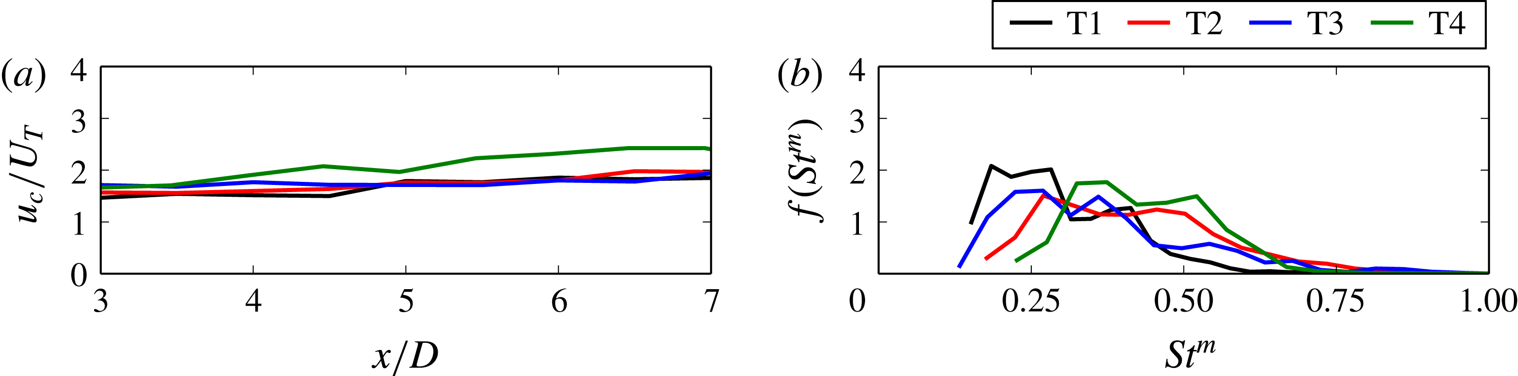
Another quantity characterising the wake meandering is the convection velocity of the meander profiles. The average convection velocity of wake meanders,
 $u_{c}$
, is calculated directly from the temporal movement of meandering profiles by obtaining the distance that the meander profile extrema travel between each time instance, as in Foti et al. (Reference Foti, Yang, Guala and Sotiropoulos2016). Figure 12(a) shows the averaged convection velocity scaled by the characteristic velocity
 $U_{T}$
, which almost collapses all profiles onto one line, indicating that the convection velocity is also related to the turbine thrust coefficient.
With the convection velocity and the wavelength of the meander profiles, we define another Strouhal number,
 $St^{m}=(u_{c}/\unicode[STIX]{x1D706})D/U_{hub}$
. Figure 12(b) shows the PDF
 $f(St^{m})$
at
 $x/D=6$
for each simulation. The PDFs are qualitatively similar and share a maximum probability around
 $St^{m}\sim 0.25$
for each turbine, which is consistent with those from spectral analysis.
(a) Meander profile average convection velocity
 $u_{c}$
. (b) Probability density function of the meander profile Strouhal number
 $f(St^{m})$
at
 $x/D=6$
.

5 Conclusions
We employed LES to investigate the wake meandering of four different wind turbines with rotor diameters spanning nearly three orders of magnitude. In our simulations, the turbine blades and nacelle were parametrised using a new actuator surface model. Similar wake meandering characteristics were observed for different turbine designs at different scales. It was found that the incoming velocity at the turbine hub height and the rotor diameter
 $D$
are the proper velocity and length scales for the mean downwind velocity deficit, the dominant frequency and the wavelength of wake meandering at far-wake locations. The turbine-added TKE, meandering amplitude and convection velocity, on the other hand, can be properly scaled by a velocity scale defined by the thrust on the rotor and the dominant frequency of the wake meandering. Furthermore, by relating the characteristic length scale
 $L_{T}$
with other known quantities as
 $L_{T}=(\sqrt{2}/2)(\sqrt{C_{T}}/St_{m})D$
, the expression shows that the meandering amplitude when normalised by
 $D$
is proportional to the thrust coefficient
 $C_{T}$
, but inversely proportional to the wake meandering frequency. For the turbine simulation cases presented, the tip-speed ratio and incoming turbulence intensity have a secondary effect on the wake meandering dynamics compared with the turbine thrust. Evidence suggests that different tip-speed ratios within the optimal power extraction turbine operating regime do not significantly affect the statistics of wake meandering, while the incoming turbulence intensity has some influence on the onset and uncertainty of wake meandering. Finally, the similarity across the turbine scales and the good agreement between model PDFs and simulations suggests that it could be possible to develop reduced-order models of wake meandering for turbines of different sizes and designs. Such an undertaking will be pursued as part of our future work.
Acknowledgements
This work was supported by the Department of Energy (DOE) (DE-EE0002980, DE-EE0005482 and DE-AC04-94AL85000) and Sandia National Laboratories. Computational resources were provided by Sandia National Laboratories and the University of Minnesota Supercomputing Institute.