2. RESEARCH OBJECTIVES AND CHALLENGES

The research objectives for a pulsar ship-based navigation system are: (i) to develop alternative algorithms for using radio pulsars based on celestial navigation methodology rather than a comparative process that matches pulse arrival times with expected ones as used by X-ray pulsar satellite navigation systems (Becker et al., Reference Becker, Kramer and Sesana2018), and (ii) to determine the accuracy of a radio pulsar ship navigation system and show that computed longitude and latitude (θ _s, φ _s) values match or exceed sextant readings and calculations.

Key challenges include: (i) radio telescope integration times required to produce a stable pulse profile, (ii) the practicality of using a timekeeping Earth-based reference system for pulsar ship-based navigation rather than the more complicated process of transferring pulsar timing measurements to a solar system barycentre (SSB) inertial reference frame as used for spacecraft navigation, (iii) identifying random number criteria for initiating Monte Carlo simulations, and (iv) providing credibility in the calculated (θ _s, φ _s) position using Monte Carlo simulations.

Pulsars are an end product of dying/exploding stars; the Crab Nebula pulsar (PSR B0531 + 21) is a classic example (Condon and Ransom, Reference Condon and Ransom2010). Pulsars are rapidly rotating and highly magnetised neutron stars that emit pulses of radiation across the whole electromagnetic spectrum (from radio to optical, X-ray and gamma ray) at their spin frequency in much the same manner as a lighthouse (Ray et al., Reference Ray, Wood and Phlips2006). Pulsars broadcast highly regular timing signals (Bernhardt et al., Reference Bernhardt, Becker, Prinz, Breithuth and Walter2011), and can be regarded as a ‘natural GPS’ (Chen, Reference Chen2018).

Many research papers, PhD theses and studies have been published addressing X-ray-based pulsar spacecraft navigation systems and pulsar timings, for example: Downs (Reference Downs1974), Sheikh et al. (Reference Sheikh, Pines, Ray, Wood, Lovellette and Wolff2006), Hecht et al. (Reference Hecht, Cahoy and Fish2016), Chen (Reference Chen2018) and Dong (Reference Dong2018). However only two studies have been identified that address radio pulsar navigation systems inside the Earth's atmosphere (Buist et al., Reference Buist, Hesselink, Gibbs, Keuning, Gaubitch, Noroozi, Bentum, Verhoeven, Heusdens, Fernandes, Kabakchiev and Kestilä2014, Reference Buist, Hesselink, Oving, Zelle, Verbeek, Noroozi, Verhoeven, Heusdens, Gaubitch, Engelen, Kestilä, Fernandes, Brito, Tavares, Kabakchiev, Kabakchiev, Vasilev, Behar and Bentum2015) and (Brito et al., Reference Brito, Fernandes and Tavares2015), and one conference presentation on using radio pulsars for ship navigation (Adamson, Reference Adamson2019).

Recent studies into pulsar navigation include NASA's X-ray experiments with a phased-array of 56 X-ray sensors on board the International Space Station (ISS). This array has an effective area of 1 m², and depending on the number of X-ray sensors used it can position the ISS to between 2 km and 19 km of its true position (Getchius et al., Reference Getchius, Long, Farahmand, Winternitz, Hassouneh and Mitchell2019; Mitchell et al., Reference Mitchell, Luke, Winternitz, Hassouneh, Price, Semper, Yu, Ray, Wolff, Kerr, Wood, Arzoumanian, Gendreau, Guillemot and Cognard2018). Studies by the European Space Agency (ESA) have shown that X-ray sensors can position interplanetary spacecraft to between 1 km and 30 km of the spacecraft's calculated position (Becker et al., Reference Becker, Kramer and Sesana2018). China's XPNAV-1 experimental satellite for X-ray pulsar observation is a forerunner for testing pulsar navigation algorithms (Zhang et al., Reference Zhang, Shuai, Huang, Chen and Xu2017).

As the Earth's atmosphere is opaque to X-rays, X-ray telescopes and sensor arrays cannot be used for ship navigation. Pulsar navigation systems for terrestrial applications and in particular pulsar ship-based navigation will have to rely on radio telescopes using frequencies ranging from 10 MHz to 40 GHz (Radio Astronomy Frequencies, 2008), with preferred frequency bands of 1400–1427, 2690–2700 and 4990–5000 MHz (ITU-R, 2013).

Most radio pulsars are very faint and can only be studied with a large radio telescope such as the 64 m diameter Parkes radio telescope which has a phased-array feed receiver system (Deng et al., Reference Deng, Chippendale, Hobbs, Johnston, Dai, George, Kramer, Karuppusamy, Malenta, Spitler, Tzioumis and Wieching2018). The Parkes telescope or a comparable telescope with a phased-array antenna (Becker et al., Reference Becker, Bernhardt and Jessner2013) is impractical for a pulsar ship navigation system due to its size, weight and cost.

Two or more radio telescopes will be required to track pulsars in different regions of the sky and produce stable pulse profiles for a 24 × 7 Pulsar ship based navigation service. An inexpensive radio telescope with a small dish or phased-array antenna is proposed, but will require a longer signal integration/observation time (Becker et al., Reference Becker, Kramer and Sesana2018). For example, a radio telescope with a 4 m dish antenna can produce a stable pulse profile with 1 h integration time (Dell'Immagine, Reference Dell'Immagine2015), while a 2 m phased-array antenna can generate a stable pulse profile within 36 min (Dong, Reference Dong2018). Although every single pulse is different, stable pulse profiles are very important for accurate pulsar timing measurements (Lorimer, Reference Lorimer2008), as they are key to providing the time difference measurement (t _ps − t _po) and hence the ship's position. The phased-array antenna option is preferred as it can track several radio sources simultaneously while the cheaper dish (e.g., parabolic) antenna can only track a single radio source (Jessner, Reference Jessner1974).

In general, the longer a pulsar is observed, the more accurately its position can be determined (Vidal, Reference Vidal2017). A position accuracy of about 2⋅5 km can be achieved by a 100 m² antenna within 10 min of integration time (Buist et al., Reference Buist, Hesselink, Gibbs, Keuning, Gaubitch, Noroozi, Bentum, Verhoeven, Heusdens, Fernandes, Kabakchiev and Kestilä2014), while a 10 km position accuracy can be achieved by a 10 m² antenna in ≈1 h integration time (Brito et al., Reference Brito, Fernandes and Tavares2015).

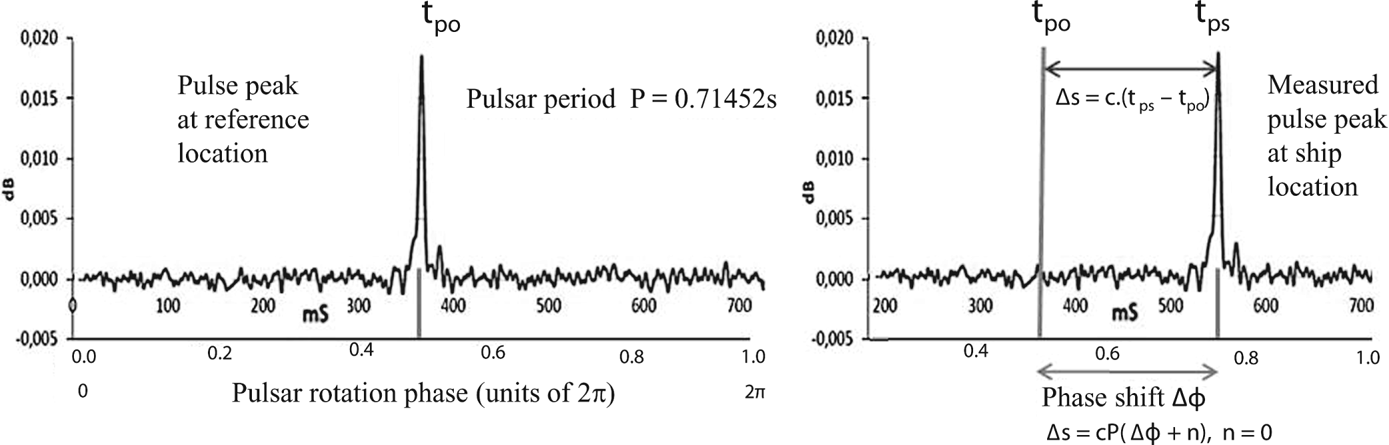
The preferred inertial frame for determining spacecraft positions is the Solar System Barycentre (SSB) frame with its origin at the centre of mass of the solar system. This reference frame is also used by the astronomical community for transferring pulsar ephemerides and precise timing information (Chen, Reference Chen2018). The position of a spacecraft can be determined with high accuracy by comparing the arrival time of the measured pulse at the spacecraft and translating it to the SSB (using the assumed position and velocity of the spacecraft), with the reference observatory's predicted pulse arrival time at the SSB. If the spacecraft position and velocity assumption is incorrect, a phase shift is observed. The pulse phase shift scheme determines a range difference Δs = c⋅P⋅(Δϕ + n) along the line of sight towards the observed pulsar, where P is the pulse period, Δϕ the phase shift, and n = 0, ±1, ±2, … is an integer that takes into account the periodicity of the observed pulses (Becker et al., Reference Becker, Bernhardt and Jessner2013).

The SSB inertial frame is inappropriate for a pulsar ship-based navigation system because additional computing resources would be required for translating pulsar ephemerides and timing information together with terrestrial position data between an Earth-based frame and the SSB frame. In this study the selected reference frame uses a stellar timekeeping system called Sidereal Time based on the Earth's rotation (Roy, Reference Roy1965), which is the preferred reference frame for celestial navigation (Nautical Almanac, 2022).

3. ASSUMPTIONS AND INITIAL CONDITIONS

For the chosen simulation, the ship's last known position was selected in the Bay of Biscay as this area is noted for its severe storms and formidable sea currents, wind and waves. Its location was geodetic longitude θ = 5⋅61°W, geodetic latitude φ = 45⋅53°N, on 8 May 2018, at 12:30 Universal Time (UT). Using drift prediction data (Météo-France, 2019), the ship's average drift velocity was 0⋅93 knots, bearing 91°, and its new (geodetic) location (S) was θ_s = 4⋅738°W, φ_s = 45⋅515°N, on 10 May 2018, UT 20:50.

Jodrell Bank Observatory (GPS location 2⋅2943808°W, 53⋅243273°N) is a key reference location for pulsar ephemerides including accurate pulse peak timing observations (Hobbs et al., Reference Hobbs, Lyne, Kramer, Martin and Jordan2004). For ease of computation, the Royal Observatory Greenwich (GPS location θ _o = 0⋅0005°W, φ _o = 51⋅476852°N), was selected as the reference location/observatory (O) instead of Jodrell Bank. The Parkes Observatory in Australia (GPS location 148⋅257383°E, −32⋅993297°S) is another reference location (Hobbs et al., Reference Hobbs, Miller, Manchester, Dempsey, Chapman, Khoo, Applegate, Bailes, Bhat, Bridle, Borg, Brown, Burnett, Camilo, Cattalini, Chaudhary, Chen, D'Amico, Kedziora-Chudczer, Cornwell, George, Hampson, Hepburn, Jameson, Keith, Kelly, Kosmynin, Lenc, Lorimer, Love, Lyne, McIntyre, Morrissey, Pienaar, J. Reynolds, Ryder, Sarkissian, Stevenson, Treloar, van Straten, Whiting and Wilson2011).

Reference locations, such as the Jodrell Bank and Parkes observatories, have pre-SSB transfer pulsar ephemerides and timing information (Chen, Reference Chen2018) which is used to determine Δs, where Δs = c⋅(t _ps − t _po). When using either observatory as the reference location, Δs will always be in the range 0 km < │Δs│ < 3,178 km (half Earth's semi-minor axis). Consider the Crab Nebula pulsar which has a pulse period of 0⋅033 s. Multiplying this pulse period by c gives a value of 9,000 km, illustrating that a phase shift scheme is not required when using the Crab pulsar or similar pulsars. Likewise, Figure 1 shows n = 0 and the time difference measurement (t _ps − t _po) is less than the pulsar period.

Figure 1.

PSR B0329 + 54 – pulse profile at 422 MHz, obtained using radio telescope with 4 m dish antenna and 1 h integration time (Dell'Immagine, Reference Dell'Immagine2015), modified by author to illustrate phase shift Δφ and timing difference (t _ps − t _po) between expected and measured pulse peak

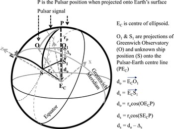
The Earth can be represented by a geoid, whose size and shape serves as a reference surface from which topographic heights and ocean depths can be measured. This geoid is not a suitable reference surface for a geometric figure of the Earth, and it is also difficult to define mathematically (Deakin and Hunter, Reference Deakin and Hunter2013). A better reference surface is an ellipsoid which is created by rotating an ellipse about its minor axis. The coordinates are geodetic longitudes and latitudes (θ, φ) and distances are geodesic arc lengths. There are an infinite number of planes that cut the surface of the ellipsoid and contain an arc between two points P and S (see Figure 2). Only one of these planes will contain the Earth's centre, and this unique plane containing the arc between points P and S is the great elliptic arc (Deakin, Reference Deakin2012).

Figure 2.

Distance Δs for calculating a ship's position

In many cases a sphere will suffice as a geometric representation of the Earth where coordinates are geocentric longitudes and latitudes (θ, $\varphi^{\prime}$). The geometric relationship between geocentric latitude ($\varphi^{\prime}$) and geodetic latitude (φ) is given by Deakin (Reference Deakin2012)

(1)\begin{equation}\tan ({\varphi^{\prime}} )= ({1-{e^2}} )\cdot \tan (\varphi )\; \; = \; \; {{b^2}/a^2} \cdot \tan (\varphi )\end{equation}

where

e = 0⋅081819191 (eccentricity)

a = 6378⋅137 km (semi-major axis)

b = 6356⋅752 km (semi-minor axis)

Applying Equation (1), the ship's new location on 10 May 2018 UT 20:50 is (θ _s = 4⋅738°W, $\varphi^{\prime}$_s = 45⋅3226°N), and the reference observatory geocentric coordinates are (θ _o = 0⋅0005°W, $\varphi^{\prime}$_o = 51⋅2892°N).

This geometric relationship is required for the simulation as celestial navigation calculations use geocentric coordinates. At the end of the simulation, the ship's calculated geocentric coordinates are translated back to geodetic coordinates as the navigator requires GNSS/GPS position data.

A sphere obeys spherical trigonometric properties, so great circle arcs SP and OP are equal to angles SE_cP and OE_cP respectively (Smart, Reference Smart1965). These are the angles subtended at the Earth's centre E_C between points S and P, and O and P. The cosine formula is a fundamental formula of spherical trigonometry which connects sides of a spherical triangle with their respective angles (Roy, Reference Roy1965). Applying the cosine formula for arc SP in spherical triangle SP_oleP (see Figure 2),

(2)\begin{equation}\begin{aligned} \cos ({\textrm{SP}} )& =\cos ({\textrm{S}{\textrm{P}_{\textrm{ole}}}} )\cos ({\textrm{P}{\textrm{P}_{\textrm{ole}}}} )\textrm{ } + \textrm{ }\sin ({\textrm{S}{\textrm{P}_{\textrm{ole}}}} )\sin ({\textrm{P}{\textrm{P}_{\textrm{ole}}}} )\cos ({\textrm{angle S}{\textrm{P}_{\textrm{ole}}}\textrm{P}} )\\ & =\cos ({\textrm{angle S}{\textrm{E}_\textrm{c}}\textrm{P}} ). \end{aligned}\end{equation}

Similarly

(3)\begin{equation}\begin{aligned} \cos ({\textrm{OP}} )& =\cos ({\textrm{O}{\textrm{P}_{\textrm{ole}}}} )\cos ({\textrm{P}{\textrm{P}_{\textrm{ole}}}} )\textrm{ } + \textrm{ }\sin ({\textrm{O}{\textrm{P}_{\textrm{ole}}}} )\sin ({\textrm{P}{\textrm{P}_{\textrm{ole}}}} )\cos ({\textrm{angle}\;\textrm{O}{\textrm{P}_{\textrm{ole}}}\textrm{P}} )\\ & =\cos ({\textrm{angle}\;\textrm{O}{\textrm{E}_\textrm{c}}\textrm{P}} ). \end{aligned}\end{equation}

Once the angles SE_cP and OE_cP are known, the value Δs (where Δs = d _o − d _s), can be calculated using right angle trigonometric functions (see Figure 2).

Determining distance Δs requires knowledge of angles subtended at the Earth's centre (see Figure 2), which is obtained by means of vector algebra or spherical trigonometry.

In vector algebra, the scalar (or dot) product of two non-zero vectors is defined as the product of the magnitudes of the two vectors and the cosine of the angle between them. If r_s r_o and r_p are non-zero vectors (see Figure 2), then the angle between these vectors can be calculated (Macbeath, Reference Macbeath1966) using

(4)\begin{equation}\cos ({\textrm{S}{\textrm{E}_\textrm{c}}\textrm{P}} )= \frac{{{\textbf{r}_\textrm{s}}.\textrm{ }{\textbf{r}_\textrm{p}}}}{{|{{\textbf{r}_\textrm{s}}} ||{{\textbf{r}_\textrm{p}}} |}} = \frac{{{d_\textrm{s}}}}{{{r_\textrm{s}}}}\quad (\textrm{see}\;\textrm{Figure}\;\textrm{2})\end{equation}

and

(5)\begin{equation}\cos ({\textrm{O}{\textrm{E}_\textrm{c}}\textrm{P}} )= \frac{{{\textbf{r}_\textrm{o}}.\textrm{ }{\textbf{r}_\textrm{p}}}}{{|{{\textbf{r}_\textrm{o}}} ||{{\textbf{r}_\textrm{p}}} |}} = \frac{{{d_\textrm{o}}}}{{{r_\textrm{o}}}}\quad (\textrm{see}\;\textrm{Figure}\;\textrm{2})\end{equation}

where

(6)\begin{equation}{\textbf{r}_\textrm{s}} \cdot {\textbf{r}_\textrm{p}} = {x_\textrm{s}} \cdot {x_\textrm{p}} + {y_\textrm{s}} \cdot {y_\textrm{p}} + {z_\textrm{s}} \cdot {z_\textrm{p}},\end{equation}

(7)\begin{equation}{\textbf{r}_\textrm{o}} \cdot {\textbf{r}_\textrm{p}} = {x_\textrm{o}} \cdot {x_\textrm{p}} + {y_\textrm{o}} \cdot {y_\textrm{p}} + {z_\textrm{o}} \cdot {z_\textrm{p}},\end{equation}

and

(x _s, y _s, z _s), (x _o, y _o, z _o) and (x _p, y _p, z _p) are the Cartesian coordinates of the ship (S), the reference observatory (O), and the pulsar position (P) when projected onto the Earth's surface.

r_s, r_o, and r_p, are radius (position) vectors of magnitude $\left|\mathbf{r}_{\mathbf{s}}\right|, \left|\mathbf{r}_{\mathbf{o}}\right|$ and $\left|\mathbf{r}_{\mathbf{p}}\right|$.

The radius (r) can be calculated for any given geocentric latitude ($\varphi^{\prime}$) using (WGS 84 GEOID-NGA)

(8)\begin{equation}r = \frac{{a{{(1{-}{e^2})}^{1/2}}}}{{{{({1{-}{e^2}\;\textrm{co}{\textrm{s}^2}\varphi^{\prime}} )}^{1/2}}}},\quad \textrm{where}\;r = |\textbf{r} |.\end{equation}

Values of a and e are given with Equation (1), above.

Many position problems in geodesy, navigation and astronomy are computed in rectangular coordinates. A number of systems are available. If an equatorial system is chosen for specifying positions on Earth, then the x,y,z geocentric Cartesian coordinate system has an origin at E _c, the centre of the ellipsoid (Deakin, Reference Deakin2012). The xE _cz plane is the Greenwich meridian plane and the xE _cy plane is the equatorial plane. The positive x-axis passes through the intersection of the Greenwich meridian and the equator, the positive y-axis is advanced 90° east along the equator, and the positive z-axis passes through the north pole of the ellipsoid (see Figure 2).

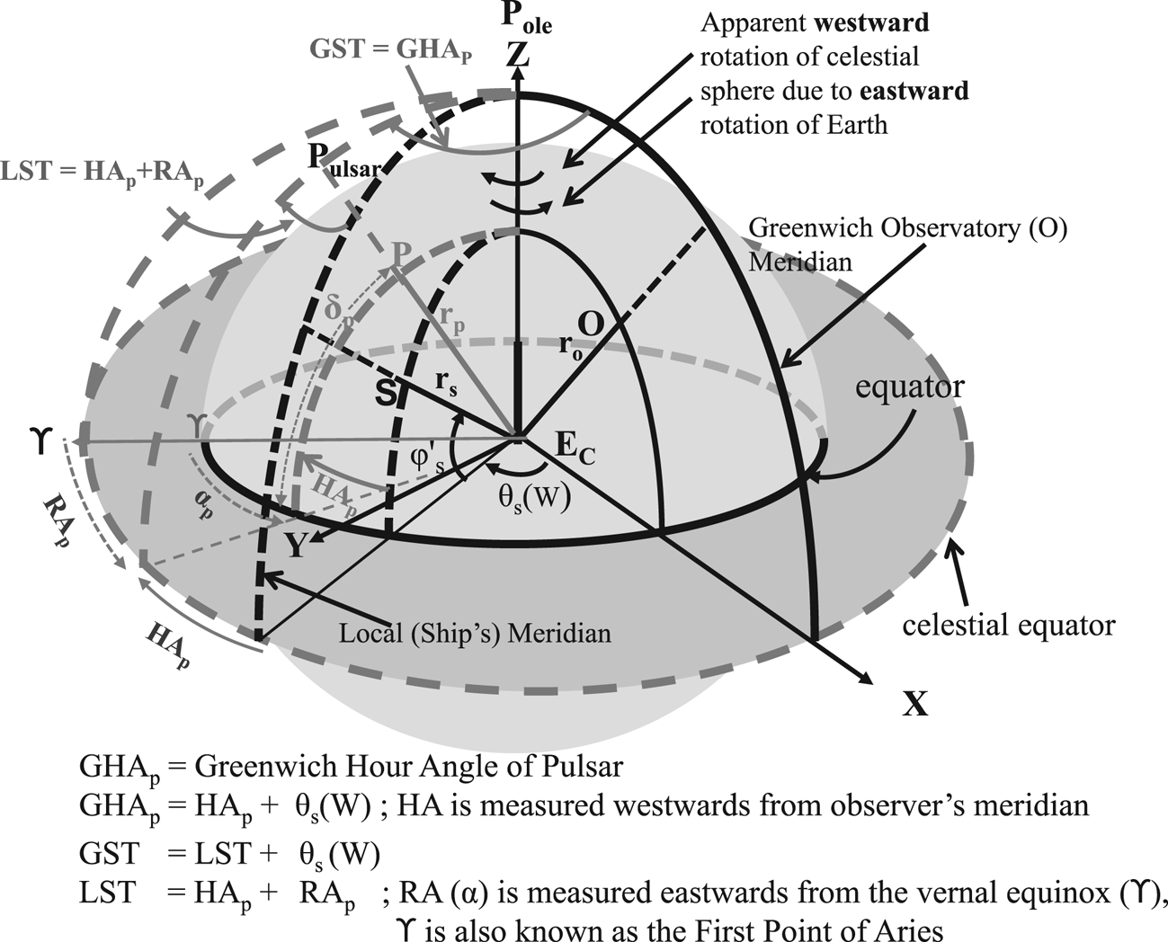
A similar equatorial system can be chosen for specifying stellar positions; the only difference being the positive y-axis is advanced 90° west along the equator (see Figure 3). All celestial bodies can be projected onto a celestial sphere with fixed right ascenion (RA, also denoted by α) and declination (δ) coordinates; these are analogous to the terrestrial longitude (θ) and geocentric latitude ($\varphi^{\prime}$).

Figure 3.

Equatorial system for specifying stellar positions

To an observer, the celestial sphere appears to rotate around the polar axis. This apparent diurnal motion introduces another coordinate system, the star's hour angle (HA) and declination (δ) which is used to determine the star's position relative to the observer's meridian (an imaginary line between north and south poles and through the local/observer's overhead position). It introduces a system of timekeeping called Sidereal Time based on the Earth's rotation where Local Sidereal Time (LST) is given by Roy (Reference Roy1965)

(9)\begin{equation}\textrm{LST} = \textrm{HA}\;\textrm{of}\;\textrm{star}\;(\textrm{e}\textrm{.g}\textrm{.}\;\textrm{Pulsar}) + \textrm{RA}\;\textrm{of}\;\textrm{star}\;(\textrm{e}\textrm{.g}\textrm{.}\;\textrm{Pulsar}).\end{equation}

Using the Greenwich prime meridian as the timekeeping reference, the relationship between Greenwich Sidereal Time (GST) and Local Sidereal Time (LST) is

(10)\begin{equation}\begin{aligned} \textrm{GST} & =\textrm{LST} + {\theta _\textrm{s}}(W);\quad 0^\circ \le \theta \le 180^\circ \;\; (\textrm{see}\;\textrm{Figure 3})\\ & =\textrm{H}{\textrm{A}_\textrm{p}} + \textrm{R}{\textrm{A}_\textrm{p}}\; + \; {\theta _\textrm{s}}(W). \end{aligned}\end{equation}

Conversely, if the longitude is east, the angle θ is subtracted.

When HA measurements are made with respect to the Greenwich meridian, timekeeping is referred to as either Greenwich Mean Sidereal Time (GMST) when the position of ϒ (Aries, see Figure 3) is affected by precession, or Greenwich Apparent Sidereal Time (GAST) when the position of ϒ is affected by precession and nutation.

Prior to the IAU2000 resolutions, GMST and GAST were defined as (Kaplan, Reference Kaplan2005)

(11)\begin{equation}\begin{aligned} \textrm{GMST} & =86400 \cdot \omega \; + (0 {\cdot} 014506 + 4612 {\cdot} 156534T + 1{\cdot}3915817{T^2}\\ & \quad - 0 {\cdot} 00000044{T^3} - 0 {\cdot} 000029956{T^4} - 0 {\cdot} 0000000368{T^5})/15\;\textrm{s} \end{aligned}\end{equation}

where

ω = 0⋅7790572732640 + 1⋅00273781191135448⋅D_U

D_U = (JD − 2,451,545) days

T = (JD − 2,451,545)/36,525

JD = Julian Date measured from fundamental epoch J2000 (January 1⋅5, 2000)

and

(12)\begin{equation}\textrm{GAST} = \textrm{GMST} + \cos (\varepsilon )\cdot \Delta \psi /15\;\textrm{s}\quad (\textrm{equation}\;\textrm{of}\;\textrm{the}\;\textrm{equinoxes})\end{equation}

where

(13)\begin{equation}\varepsilon = \textrm{mean}\;\textrm{obliquity}\;\textrm{of}\;\textrm{the}\;\textrm{ecliptic}\;({{\varepsilon_0}} )+ \textrm{nutation}\;\textrm{in}\;\textrm{obliquity}({\Delta \varepsilon } )\end{equation}

\[{\varepsilon _0} = 84381{\cdot}406\;\textrm{arc}\;\textrm{seconds}\]

\[\begin{aligned} \Delta \varepsilon & =- 46{\cdot}836769T - 0{\cdot}0001831{T^2} + 0{\cdot}00200340{T^3}\\ & \quad - 0{\cdot}000000576{T^4} - 0{\cdot}0000000434{T^5}\;\textrm{arc}\;\textrm{seconds}\textrm{.} \end{aligned}\]

A simplified expression for Δψ is given by Meeus (Reference Meeus1998) and Seeber (Reference Seeber2003)

(14)\begin{equation}\Delta \psi ={-} 17{\cdot}20\;\textrm{sin}\;\Omega - 1{\cdot}32\;\textrm{sin}\;2L - 0{\cdot}23\;\textrm{sin}\;2L^{\prime} + 0{\cdot}21\;\textrm{sin}2\Omega \quad \textrm{arc}\;\textrm{seconds}\end{equation}

while Ω, L and $L^{\prime}$ are defined by

\[\begin{array}{l} \Omega = 125^\circ{\cdot} 04452 - 1934 {\cdot} 136261T + 0{\cdot}0020708{T^2} + {T^3}/450,000\;\textrm{degrees}\\ L = 280^\circ{\cdot} 4665 + 36,000^\circ{\cdot} 76983T + 0{\cdot}0003032{T^2}\;\textrm{degrees}\\ L^{\prime} = 218^\circ{\cdot} 3165 + 481,267^\circ{\cdot} 8813T\;\textrm{degrees}\textrm{.} \end{array}\]

The computed value for Δψ is accurate to 0⋅5 arc seconds.

For UT 20:50 on 10 May 2018, GMST and GAST were calculated to be

\[\textrm{GMST} = 181{\cdot}1033\;\textrm{degrees}\]

\[\textrm{GAST} = 181{\cdot}0996\;\textrm{degrees}\textrm{.}\]

The pulsar's HA_p can be calculated using Equation (10). As GST = GAST (Capitaine and Wallace, Reference Capitaine and Wallace2009), and GLST = GST, re-arranging Equation (10) gives

(15)\begin{equation}\textrm{H}{\textrm{A}_\textrm{p}} = \textrm{GAST} - \{{\textrm{R}{\textrm{A}_\textrm{p}} + {\theta_\textrm{o}}(W )} \};\quad \textrm{where}\;{\theta _\textrm{o}}(W )\approx 0^\circ .\end{equation}

Alternatively, the IAU2000 (Capitaine and Wallace, Reference Capitaine and Wallace2009) and IAU2006 (Wallace and Capitaine, Reference Wallace and Capitaine2006) resolutions provide a highly accurate expression for GST in terms of the Earth's rotation angle (ERA ≡ GMST) and equation of the origins (EO).

Several Pulsars were selected for illustrative purposes (see Table 1) from a catalogue of 374 pulsars obtained from archival data stored at Jodrell Bank Observatory (Hobbs et al., Reference Hobbs, Lyne, Kramer, Martin and Jordan2004), as they could be observed from the ship's location (S) on 30 May 2018, UT 20:50.

Table 1.

Selected pulsar coordinates for the simulation, epoch 2000 and 2018

In practice, millisecond pulsars (MSPs) such as the Crab Nebula pulsar are preferred for spacecraft navigation simulations/experiments because of their stable pulse profile obtained over a period of integration time, and their signal strength (Bernhardt et al., Reference Bernhardt, Becker, Prinz, Breithuth and Walter2011). However, ≈7% of known pulsars are MSPs; some MSPs will be within the ship's observable horizon, while others may not be suitable. The Crab Nebula pulsar was not chosen as its position was below the ship's observable horizon.

Table 1 shows the Pulsar J2000 notation followed by the right ascension (RA_p) and declination (δ _p) coordinates for standard epoch 2000. The pulsar coordinates were then corrected (coordinate reduction) to obtain their apparent position on 10 May 2018, UT 20:50. Coordinate reduction between the two epochs requires proper motion, precession, nutation, annual aberration, annual parallax and gravitational deflection of light (Meeus, Reference Meeus1998).

Table 2 provides true data values for the ship's location on 10 May 2018, UT 20:50. Pulsar hour angles (HA_p) are calculated using Equation (15) and pulsar RA_p coordinates are provided in Table 1.

Table 2.

True data values at ship's new location (θ _s = 5⋅738°W, $\varphi^{\prime}$_s = 45⋅323°N) for UT 20:50 10 May 2018

Equation (8) was used to calculate the true radius values r _s, r _o and r _p on 10 May 2018, UT 20:50 using geocentric latitudes ($\varphi^{\prime}$_s, $\varphi^{\prime}$_o) for the ship's new location and Greenwich Observatory, and the pulsar's projected position on the Earth's surface using its declination δ _p (see Table 1). Radius values for r _s and r _o are 6,367⋅297 km, and 6,365⋅090 km, values for r _p are provided in Table 2.

Angles (SE_cP) and (OE_cP) were obtained using Equations (2) and (3). Distances d_o and d_s could then be calculated using Equations (4) and (5), followed by Δs (see Figure 2 and Table 2), where Δs = d _o − d _s. Finally the true pulse peak time difference values (t _ps − t _po) observed at the ship's location were obtained by dividing Δs by c.

Having calculated the initial conditions/data values (see Table 2), the ship's longitude and latitude coordinates could be calculated by reverse engineering. The following assumptions were made to obtain simulated data values prior to calculating (θ _s, $\varphi^{\prime}$_s).

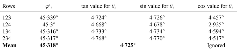
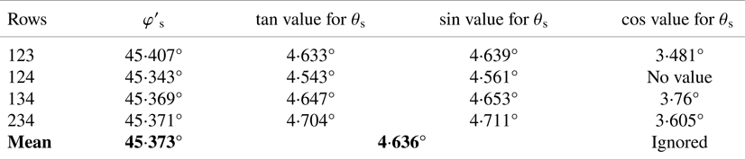
Pulsars J1321 + 8323 and J1115 + 5030 were used with caution. First, their declinations were either too close to 90° or too similar to the ship's latitude (see Table 2). For example, pulsar stellar coordinates, namely hour angle (analogous to longitude) and declination (analogous to latitude) whose values are too close to 90° or too similar to the ship's coordinates, may produce trigonometric values close to zero, or numerical values that are multiplied by or divisible by values close to zero. Second, the value of Δs may be an order of magnitude less than the other Δs values (see Table 2). In both instances this could lead to a loss of significant figures or anomalies, thus giving unreliable values (e.g., see cos value for θ _s in Tables 5 and 6).

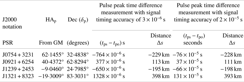
Pulse peak time difference measurements were assumed to be within 3 × 10⁻⁶ s and 2 × 10⁻⁵ s for a four-pulsar ship-based navigation system, and 3 × 10⁻⁶ s for a single-pulsar ship-based navigation system.

A random number generator supplied a pulse peak time difference measurement between upper and lower timings. Consider a time difference measurement of −7.6558 × 10⁻⁴ s for Pulsar J0754 + 3231 (see Table 2). Assuming a timing accuracy of 3 × 10⁻⁶ s, the upper and lower timings will be −7.6258 × 10⁻⁴ s and −7.6858 × 10⁻⁴ s. A random number within this range is −7.64 × 10⁻⁴ s, which provides a unique starting value/seed for an Excel calculation or a Monte Carlo simulation cycle, and when multiplied by c provides Δs = −229 km (see Table 3).

Table 3.

Random number generated (i.e., simulated) data values to calculate ship's position for UT 20:50 10 May 2018

For statistical purposes, a credible ship's velocity was set at ≤25 knots. Bearing values between 180° and 360° were discarded as the ship is drifting eastwards.

Distances r _o, r _p, d _o, and d _s were rounded to the nearest kilometre as the simulated ship's location (θ _s, $\varphi^{\prime}$_s) was expected to be ≤10 km (Brito et al., Reference Brito, Fernandes and Tavares2015) of its true location. The target accuracy for the experiments was to match or exceed sextant readings and calculations by positioning the ship to within 2 km of its new location.

The ship's distance r _s was taken to equal the ship's last known distance from the Earth's centre, giving r _s = 6367 km when rounded to the nearest kilometre. This is a valid assumption as the expected change in r _s is minimal; it also reduces the computational problem to solving two equations for the unknowns (θ _s, $\varphi^{\prime}$_s).

Finally it is assumed that: (i) relevant technology exists to detect radio signals from at least three simultaneous distinct pulsars visible from the ship's observable horizon (see Table 1), (ii) the ship's clock keeps UT to the required accuracy, (iii) stable pulse profiles are obtainable using a radio telescope with a 4 m dish antenna or a 2 m phased array antenna requiring ≤1 h integration period, (iv) pulse peak time difference measurements can be resolved within the required accuracy for ship velocities ≤25 knots.

4. FOUR-PULSAR SHIP-BASED NAVIGATION

A four-pulsar ship-based navigation system will produce an over-determined solution providing at least four solutions for the two unknowns (θ _s, $\varphi^{\prime}$_s). This is based on the assumption that the ship's distance r_s is equal to the ship's last known value on 8 May 2018, UT 12:30.

The following steps were undertaken to simulate the ship's most likely position based on four time difference measurements of (t _ps − t _po) seconds on 10 May 2018, UT 20:50. Multiplying (t _ps − t _po) by c provides four distance values for Δs which are fundamental in calculating a ship's position.

• Step 1 A random number generator supplied pulse peak time difference measurements (t _ps − t _po) between the ship and the selected reference location. These simulated measurements provided a unique starting value/seed for an Excel calculation or a Monte Carlo simulation cycle (see Table 3).

The distance value Δs was obtained using Δs = c⋅(t _ps − t _po).

• Step 2 Pulsar coordinates (α _p, δ _p) were updated for epoch 10 May, UT 20⋅50, 2018 (see Tables 1 and 2) using coordinate reduction. HA_p and the magnitude of the pulsar's position vector when projected onto the Earth's surface $\left|\mathbf{r}_{p}\right|$ were calculated using Equations (8) and (11)–(15). Both HA_p and r _p values are provided in Table 2.

• Step 3 d _o was calculated using

  \[{d_\textrm{o}} = {r_\textrm{o}}\;\textrm{cos}({\textrm{O}{\textrm{E}_\textrm{c}}\textrm{P}} )\quad ({\textrm{see}\;\textrm{Figure 2}} )\]
  where
  \[{r_\textrm{o}} = 6365\;\textrm{km}\;({\textrm{radius}\;\textrm{rounded}\;\textrm{to}\;\textrm{nearest}\;\textrm{kilometre}} )\]
  and
  \[\textrm{cos}({\textrm{O}{\textrm{E}_\textrm{c}}\textrm{P}} )= \frac{{{\textbf{r}_\textrm{o}}.{\textbf{r}_\textrm{p}}}}{{|{{\textbf{r}_\textrm{o}}} ||{{\textbf{r}_\textrm{p}}} |}} = \frac{{{d_o}}}{{{r_\textrm{o}}}}\quad (see\;\textrm{Equations}\;(5)\;\textrm{and}\;(7)).\]

Values for d _o (see Table 2), were rounded to the nearest kilometre.

• Step 4 A set of four equations were now generated for the unknown (θ _s, $\varphi^{\prime}$_s). Starting with the expression for d _s (see Figure 2)

  \[{d_\textrm{s}} = {d_\textrm{o}} - \Delta s = {r_\textrm{s}}\;\textrm{cos}({\textrm{S}{\textrm{E}_\textrm{c}}\textrm{P}} )\quad (\textrm{see}\;\textrm{Equation}\;\textrm{(}4))\]
  where
  \[{r_\textrm{s}} = 6367\;\textrm{km}\textrm{.}\]

Replacing cos(SE_cP) with Equation (2) provides

(16)\begin{equation}{d_\textrm{s}} = {d_\textrm{o}} - \Delta s = 6367[{\textrm{sin}({{{\varphi^{\prime}}_\textrm{s}}} )\textrm{sin}({{\delta_\textrm{p}}} )+ \textrm{cos}({{{\varphi^{\prime}}_\textrm{s}}} )\textrm{cos}({{\delta_\textrm{p}}} )\;\textrm{cos}({\textrm{H}{\textrm{A}_\textrm{p}} - {\theta_\textrm{s}}} )} ].\end{equation}

Noting that the sign of HA_p is determined by Equation (10), where

\[\cos ({\textrm{H}{\textrm{A}_\textrm{p}} - {\theta_s}} )= \cos ({\textrm{H}{\textrm{A}_\textrm{p}}} )\cos ({{\theta_\textrm{s}}} )+ \sin ({\textrm{H}{\textrm{A}_\textrm{p}}} )\sin ({{\theta_\textrm{s}}} ),\]

and writing a = sin($\varphi^{\prime}$_s), b = cos($\varphi^{\prime}$_s), f = cos(θ _s), g = sin(θ _s), Equation (16) becomes

(17)\begin{equation}{d_\textrm{s}} = {d_\textrm{o}} - \Delta s = 6367[{a \cdot \sin ({{\delta_\textrm{p}}} )+ b \cdot \cos ({{\delta_\textrm{p}}} )\cdot \{{f \cdot \cos ({\textrm{H}{\textrm{A}_\textrm{p}}} )+ g \cdot \sin ({\textrm{H}{\textrm{A}_\textrm{p}}} )} \}} ].\end{equation}

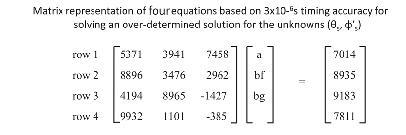
Substituting values for Δs, δ _p, HA_p (see Table 3) and d _o (see Table 2) into Equation (17), we obtain four equations for (θ _s, $\varphi^{\prime}$_s) which can be written in matrix form as in Table 4.

Table 4.

Matrix representation of four equations based on 3 × 10⁻⁶ s timing accuracy for solving an over-determined solution for the unknowns (θ _s, $\varphi^{\prime}$_s)

The simplest approach is to create four determinant solutions with row combinations 123, 124, 134, and 234.

Solving for a provides $\varphi^{\prime}$_s = 45⋅339°N. Dividing ‘bg’ by ‘bf’ provides a tan(θ _s) expression, giving a unique value θ _s = 4⋅724°W. Alternatively, substituting $\varphi^{\prime}$_s = 45⋅339° into ‘b’ provides solutions for ‘bf’ and ‘bg’ giving values θ _s = 4⋅457°W and 4⋅726°W. The correct value for θ _s is obtained by comparing with the tan solution (see Table 5).

Table 5.

Calculated position for UT 20:50, 10 May 2018 using over-determined solution based on 3 × 10⁻⁶ s timing accuracy

A third approach, which is not explored in this paper, makes use of the relationship sin² + cos² = 1, enabling ‘bg’ to be replaced by bg = b⋅√(1 − f ²). This will require the solution of second-order (quadratic) equations providing four solutions for $\varphi^{\prime}$_s, and eight solutions for θ _s.

For comparison, the usual GNSS approach in the satellite navigation domain is to express positions in Cartesian (X, Y, Z) coordinates. Solving an over-determined solution requires linearisation and an iteration process using least squares adjustments to estimate the unknowns (Langley, Reference Langley1991).

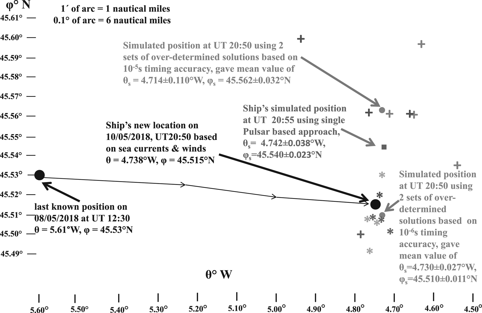
The process using 2 × 10⁻⁵ s timing accuracy was repeated using Steps 1–4 to obtain four equations for the unknowns (θ _s, $\varphi^{\prime}$_s). Results are summarised in Table 6. Steps 1–4 were repeated with different starting values/seeds for the two timing accuracies to provide additional sets of data and confidence in the simulated (θ _s, $\varphi^{\prime}$_s) results (see Figure 4).

Figure 4.

Ship's simulated geodetic positions on 10 May 2018

Table 6.

Calculated position for UT 20:50, 10 May 2018 using over-determined solution based on 2 × 10⁻⁵ s timing accuracy

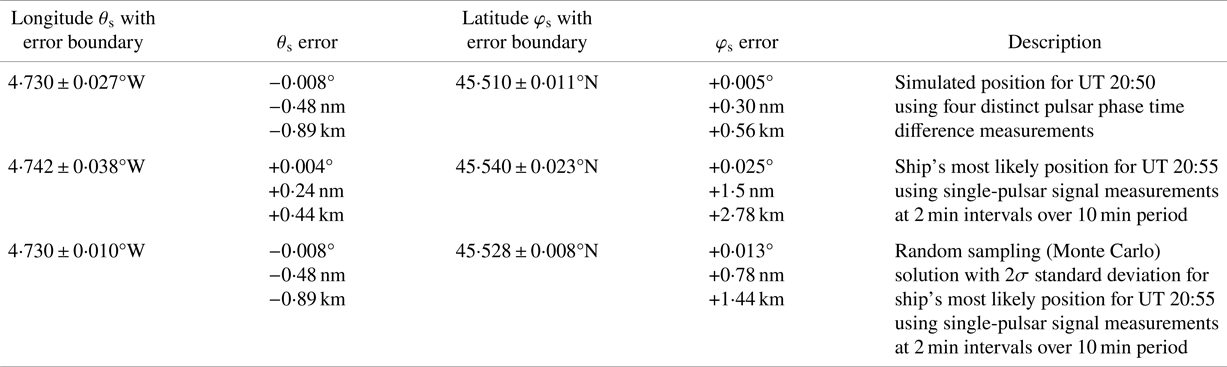
Using a least squares approach, the ship's position based on 3 × 10⁻⁶ s timing accuracy produced a mean value with σ standard deviation of (θ _s = 4⋅730 ± 0⋅027°W, $\varphi^{\prime}$_s = 45⋅318 ± 0⋅011°N). The lower timing resolution of 2 × 10⁻⁵ s provided a mean value with σ standard deviation of (θ _s = 4⋅714 ± 0⋅110°W, $\varphi^{\prime}$_s = 45⋅370 ± 0⋅032°N). Converting these positions to geodetic coordinates using Equation (1) provided (θ _s = 4⋅730 ± 0⋅027°W, φ _s = 45⋅510 ± 0⋅011°N) and (θ _s = 4⋅714 ± 0⋅110°W, φ _s = 45⋅562 ± 0⋅032°N) respectively (see Figure 4). Comparing these positions with the ship's new location (θ _s = 4⋅738°W, φ _s = 45⋅515°N) gave position errors of ≈1⋅1 km and ≈4 km.

5. SINGLE-PULSAR SHIP-BASED NAVIGATION SYSTEM

A single-pulsar-based approach was also considered because: (i) a radio telescope with a 4 m dish or a 2 m phased-array antenna is more affordable, (ii) there is limited space on a ship's superstructure for positioning a radio telescope, (iii) there may be insufficient MSPs within the ship's observable horizon for a four-pulsar system and (iv) NASA and ESA are conducting space-based X-ray navigation experiments using single pulsars.

Pulsar J0754 + 3231 was selected for illustrative purposes. It was assumed that a single-pulsar ship-based navigation system requires a pulse peak time difference measurement every 2 min over a 10 min period providing six equations/solutions for (θ _s, $\varphi^{\prime}$_s). The simulated pulse peak time difference measurements took into account a slow moving ship (in our scenario, the ship is assumed to be stationary as 0⋅93 knot drift velocity equates to 0⋅3 km distance in 10 min, which is negligible when compared with the target accuracy of ≈2 km) and the pulsar's diurnal motion, while a least squares best fit linear equation optimised (θ _s, $\varphi^{\prime}$_s) for UT 20:55.

The following steps were undertaken to calculate the ship's most likely position for UT 20:55, 10 May 2018, based on a pulsar peak timing accuracy of 3 × 10⁻⁶ s.

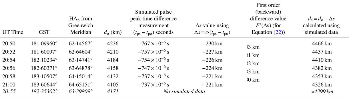
Steps 1–3 were reused to calculate (i) time differences (t _ps − t _po) and Δs, (ii) GST, updated pulsar coordinates (α _p, δ _p) using coordinate reduction, and HA_p using Equations (11)–(15), and (iii) d _o at 2 min intervals from UT 20⋅50 to 21:00, 10 May 2018 (see Table 7). The value r _p (see Table 2) remained unchanged over the 10 min period.

Table 7.

Random number generated (simulated) data to calculate ship's position at 2 min time intervals using pulsar J0754 + 3231 (α _p = 118⋅95493°, δ _p = 32⋅48383°), for UT 20:55, 10 May 2018 with signal timing accuracy of 3 × 10⁻⁶ s

Step 4 Angle (SE_cP) was calculated using

\[{d_\textrm{s}} = {r_\textrm{s}}\;\cos ({\textrm{S}{\textrm{E}_\textrm{c}}\textrm{P}} )= {d_\textrm{o}} - \Delta s\quad (\textrm{see}\;\textrm{Equation}\;\textrm{(4)}\;\textrm{\& }\;\textrm{Figure}\;\textrm{2)}\]

where

\[{r_\textrm{s}} = 6367\;\textrm{km}.\]

Step 5 Replacing cos (SE_cP) with Equation (2),

\[{d_\textrm{s}}/{r_\textrm{s}} = \cos ({\textrm{S}{\textrm{E}_\textrm{c}}\textrm{P}} )= \sin ({{{\varphi^{\prime}}_\textrm{s}}} )\sin ({{\delta_\textrm{p}}} )+ \cos ({{{\varphi^{\prime}}_\textrm{s}}} )\cos ({{\delta_\textrm{p}}} )\cos ({\textrm{H}{\textrm{A}_\textrm{p}} - {\theta_s}} ).\quad (\textrm{see}\;\textrm{Equation}\;\textrm{(16)})\]

Re-arranging

(18)\begin{equation}\cos ({\textrm{H}{\textrm{A}_\textrm{p}} - {\theta_s}} )= [{\cos ({\textrm{S}{\textrm{E}_\textrm{c}}\textrm{P}} )- \sin ({{{\varphi^{\prime}}_\textrm{s}}} )\sin ({{\delta_\textrm{p}}} )} ]/\cos ({{{\varphi^{\prime}}_\textrm{s}}} )\cos ({{\delta_\textrm{p}}} ).\end{equation}

Step 6 Equation (18) was used as a predictor-corrector algorithm for solving (θ _s, $\varphi^{\prime}$_s); this is analogous to predictor-corrector algorithms for numerical computations (Adamson, Reference Adamson1976).

The starting point (‘predictor’ component) is calculating angle (HA_p − θ _s); obtained by substituting $\varphi^{\prime}$_s = 45⋅3376° (the ship's last known geocentric latitude) together with angle (SE_cP) and δ _p = 32⋅4838° (see Table 7) into Equation (18).

θ _s is obtained by subtracting (HA_p − θ _s) from the pulsar's hour angle provided in Table 7.

Step 7 Equation (19) is a re-arranged Equation (18). Substituting angle (HA_p − θ _s), δ _p and angle (SE_cP) into Equation (19) provides a solution for $\varphi^{\prime}$_s (‘corrector’ component) as follows

(19)\begin{equation}0 = \sin ({{{\varphi^{\prime}}_\textrm{s}}} )\sin ({{\delta_\textrm{p}}} )+ \cos ({{{\varphi^{\prime}}_\textrm{s}}} )\cos ({{\delta_\textrm{p}}} )\cos ({\textrm{H}{\textrm{A}_\textrm{p}} - {\theta_\textrm{s}}} )- \cos ({\textrm{S}{\textrm{E}_\textrm{c}}\textrm{P}} ).\end{equation}

Writing f = sin(δ _p), g = cos(δ _p)cos(HA_p − θ _s), h = cos(SE_cP), and noting that

\[{\sin ^2}({{{\varphi^{\prime}}_\textrm{s}}} )\textrm{ } + \textrm{ }{\cos ^2}({{{\varphi^{\prime}}_\textrm{s}}} )= 1,\quad \textrm{Eq}\textrm{.}\;\textrm{(19)}\;\textrm{reduces}\;\textrm{to}\;\textrm{a}\;\textrm{quadratic}\;\textrm{equation}\;\textrm{of}\;\textrm{form}\]

\[0 = f \cdot \sin ({{{\varphi^{\prime}}_\textrm{s}}} )\textrm{ } + \textrm{ }g \cdot \surd [1\textrm{ }{-}\textrm{ }{\sin ^2}({{{\varphi^{\prime}}_\textrm{s}}} )] - h.\]

Re-arranging,

\[0 = ({{f^2} + {g^2}} )\cdot {\sin ^2}({\varphi ^{\prime}_\textrm{s}}) - 2fh \cdot \sin ({\varphi ^{\prime}_\textrm{s}}) + ({{h^2} - {g^2}} ).\]

Writing

\[a = ({{f^2} + {g^2}} ),\;b ={-} 2fh,\;c = ({{h^2} - {g^2}} ),\]

Equation (19) becomes

\[0 = a \cdot {\sin ^2}({\varphi ^{\prime}_s}) + b \cdot \sin ({\varphi ^{\prime}_s}) + c,\]

whose solution is

\[\sin ({\varphi ^{\prime}_\textrm{s}}) = [{ - b \pm \surd ({{b^2} - 4ac} )} ]/2a.\]

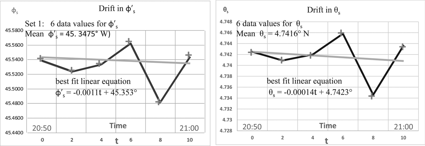
Step 8 Steps 1–7 were repeated every 2 min over a period of 10 min, providing six solutions for θ _s and two sets of six solutions for $\varphi^{\prime}$_s. Only one set of solutions for $\varphi^{\prime}$_s provided plausible drift velocity and bearing (see Figure 5).

Figure 5.

Drift in ship's longitude and latitude at 2 min intervals for a period of 10 min from UT 20:50 to 21:00, 10 May 2018 using pulsar J0754 + 3231

Step 9 Steps 1–7 were now repeated six times using θ _s = 5⋅61° (the last known longitude value of the ship) as the starting point in Step 7 to obtain $\varphi^{\prime}$_s. The value of $\varphi^{\prime}$_s was then used in Step 6 to obtain θ _s. This provided unconvincing mean longitude and latitude values of (θ _s = 4⋅9157°W, $\varphi^{\prime}$_s = 44⋅1017°N). The least squares best fit linear equations for (θ _s, $\varphi^{\prime}$_s) also provided implausible drift velocity and bearing. Of the two solutions, the first provided the ship's most likely position as (θ _s = 4⋅7416°W, $\varphi^{\prime}$_s = 45⋅3475°N).

A differential correction method was used to calculate the incremental values δ(θ _s) and δ($\varphi^{\prime}$_s) which defined the position error for (θ _s, $\varphi^{\prime}$_s) as θ _s = 4⋅742 ± δ(θ _s)°, $\varphi^{\prime}$_s = 45⋅348 ± δ($\varphi^{\prime}$_s)° for UT 20:55.

Starting with d _s (see Figure 2), in functional format d _s is expressed as

\[{d_\textrm{s}} = F({{x_\textrm{p}},\textrm{ }{y_\textrm{p}},\textrm{ }{z_\textrm{p}},\textrm{ }{x_\textrm{s}},\textrm{ }{y_\textrm{s}},\textrm{ }{z_\textrm{s}}} ).\]

There is no dependency on ($\dot{x}_{s}$, $\dot{y}_{s}$, $\dot{z}_{s}$) as the dimension of d _s is [L], and ($\dot{x}_{s}$, $\dot{y}_{s}$, $\dot{z}_{s}$) is [LT⁻¹].

Converting (x _s, y _s, z _s) to spherical coordinates and noting that the dependency on r _s can be ignored (the incremental change in r _s is in the order of centimetres), d _s can be re-written in functional format as

\[{d_\textrm{s}} = F({{\theta_\textrm{s}},{{\varphi^{\prime}}_\textrm{s}}} ).\]

Using Taylor's theorem for two variables, the first approximation for the incremental change in (θ _s, $\varphi^{\prime}$_s) can be written as

(20)\begin{equation}F^{\prime}({{d_\textrm{s}}} )= F^{\prime}({{d_\textrm{o}} - \Delta s} )={-} F^{\prime}({\Delta s} )= \frac{{\partial ({{d_\textrm{s}}} )}}{{\partial ({{\theta_\textrm{s}}} )}} \cdot F^{\prime}({{\theta_\textrm{s}}} )\textrm{ } + \textrm{ }\frac{{\partial ({{d_\textrm{s}}} )}}{{\partial ({{\varphi ^{\prime}}_\textrm{s}})}} \cdot F^{\prime}({\varphi ^{\prime}_\textrm{s}})\end{equation}

where

(21)\begin{equation}\begin{aligned} {d_\textrm{s}} & =\{{{x_\textrm{p}} \cdot {x_\textrm{s}} + {y_\textrm{p}}.{y_\textrm{s}} + {z_\textrm{p}} \cdot {z_\textrm{s}}} \}/|{{\textbf{r}_\textrm{p}}} |\\ & =\{{{x_\textrm{p}}.[{r_\textrm{s}}\cos ({{\varphi^{\prime}}_\textrm{s}})\cos ({\theta_\textrm{s}})] + {y_\textrm{p}}.[{r_\textrm{s}}\cos ({{\varphi^{\prime}}_\textrm{s}})\sin ({\theta_\textrm{s}})] + {z_\textrm{p}}.[{r_\textrm{s}}\sin ({{\varphi^{\prime}}_\textrm{s}})]} \}/|{{\textbf{r}_\textrm{p}}} |\end{aligned}\end{equation}

and $F^{\prime}$(d _o) = 0, as there is no incremental change in d _o

Hence

(22)\begin{equation}\begin{aligned} - F^{\prime}({\Delta s} )& =F^{\prime}({{\theta_\textrm{s}}} )\cdot \{ - \textrm{ }{x_\textrm{p}} \cdot [{r_\textrm{s}}\;\cos ({{\varphi ^{\prime}}_s})\sin ({\theta _s})] + {y_p} \cdot [{r_\textrm{s}}\;\cos ({{\varphi ^{\prime}}_s})\cos ({\theta _\textrm{s}})]\} /|{{{\bf r}_\textrm{p}}} |\\ & \quad + \textrm{ }F^{\prime}({{\varphi ^{\prime}}_\textrm{s}}).\{ - \textrm{ }{x_\textrm{p}}.[{r_\textrm{s}}\sin ({{\varphi ^{\prime}}_\textrm{s}})\cos ({\theta _\textrm{s}})] - {y_\textrm{p}} \cdot [{r_s}\sin ({{\varphi ^{\prime}}_\textrm{s}})\sin ({\theta _\textrm{s}})]\\ & \quad + \textrm{ }{z_\textrm{p}} \cdot [{r_\textrm{s}}\;\textrm{cos}({{\varphi ^{\prime}}_\textrm{s}})]\} /|{{{\bf r}_\textrm{p}}} |. \end{aligned}\end{equation}

Since ${\rm F}^{\prime}$(θ _s) ≡ δ(θ _s) and ${\rm F}^{\prime}$($\varphi^{\prime}$_s) ≡ δ($\varphi^{\prime}$_s), and using the values of $F^{\prime}$(Δs) provided in Table 7, the incremental change (i.e., position error) gave the ship's most likely position as (θ _s = 4⋅742 ± 0⋅038°W, $\varphi^{\prime}$_s = 45⋅348 ± 0⋅023° N) for UT 20:55. There was confidence in these results as the ship's new location lay within the calculated position error.

Monte Carlo simulations using Pulsar J0754 + 3231 added further confidence (see Table 8). A random number generator supplied pulse peak time difference measurements as the input seed for each program cycle. The resultant mean position (with 2σ standard deviation) for UT 20:55 was (θ _s = 4⋅730 ± 0⋅010°W, $\varphi^{\prime}$_s = 45⋅336 ± 0⋅008°N). Analysing each cycle showed that 15% to 25% of the overall cycles provided potentially credible velocity and bearing values of ≈15 knots and ≈165° respectively. The remaining cycles provided non-credible velocities of >25 knots and incorrect bearings of ≈350°.

Table 8.

Ship's simulated geodetic position compared with ship's new location for 10 May 2018 using a pulsar signal timing resolution of 3 × 10⁻⁶ s

Geodetic positions are provided in Figure 4 and Table 8.

Additional Monte Carlo simulations with Pulsars J0921 + 6254 and J1115 + 5030 gave the ship's position as (θ _s = 4⋅741 ± 0⋅027°W, $\varphi^{\prime}$_s = 45⋅338 ± 0⋅0002°N) and (θ _s = 4⋅709 ± 0⋅076°W, $\varphi^{\prime}$_s = 45⋅337 ± 0⋅005°N) respectively, thus supporting the Pulsar J0754 + 3231 results.