


1 Introduction
Example (1a) exemplifies a positive construction: a construction containing an unmodified gradable adjective. Example (1b) exemplifies a comparative.

There is an important difference between the two constructions, one that has been central to a longstanding debate about the semantics of gradable adjectives: while (1a) entails that John counts as significantly tall in the context of interpretation, (1b) does not. In other words, (1b) but not (1a) is acceptable in a context in which John does not qualify as tall.
Intuitively, it is the adjective tall in (1a) that contributes this ‘taller than average’ or ‘significantly tall’ meaning, which we will refer to as ‘evaluativity’.Footnote [2] However, as Klein (Reference Klein1980) has pointed out, the difference between (1a) and (1b) poses a problem for a compositional semantics of adjectival constructions: if evaluativity is lexically encoded in the adjective tall, what suppresses it in the comparative in (1b)? Or, if it is not, what introduces it in the positive construction in (1a)?
Since Klein’s discussion (and preceding work in Bartsch & Vennemann Reference Bartsch and Vennemann1972, Kamp Reference Kamp and Keenan1975, Cresswell Reference Cresswell and Partee1976), evaluativity remains a central issue for the semantics of adjectival constructions (and, consequently, degree semantics generally), and it remains a central member of the class of context-sensitive phenomena. Evaluativity has been argued to vary across adjectival classes (Rotstein & Winter Reference Rotstein and Winter2004, Kennedy & McNally Reference Kennedy and McNally2005), across adjectival constructions (Bierwisch Reference Bierwisch, Bierwisch and Lang1989, Rett Reference Rett2008b) and in how it contributes semantically to a context of utterance (Barker Reference Barker2002, Rett Reference Rett2015).
As it stands, the discussion of the distribution and contribution of evaluativity has been largely relegated to the theoretical literature.Footnote [3] The goal of this paper is to present some initial forays into an experimental investigation of the distribution and contribution of evaluativity. We take for granted Bierwisch’s (Reference Bierwisch, Bierwisch and Lang1989) claim that evaluativity is not distributionally restricted to the positive construction, and we focus on two other questions. First, how, if at all, do relative and absolute adjectives behave differently across constructions with respect to evaluativity? Second, how, if at all, does context play a role in the distribution of evaluativity across adjectival constructions?
We begin in Section 2 by reviewing evaluativity generally, as well as the various adjectival classes and constructions included in the experiment. In Section 3, we present a series of experiments intended to address the first question, about the effect of adjective class on evaluativity. After discussing a particularly surprising result of these experiments (and the history of this result in the psychology literature, in Section 3.2.4), we present in Section 4 a third experiment designed to follow up on the first two by further probing the role of context in the distribution of evaluativity (the second question). While our results are in general consistent with previous claims about evaluativity, they suggest that the phenomenon is idealized in the theoretical literature: evaluativity arises in some circumstances as a pragmatic inference, and it seems to be more gradable than categorical.
2 Evaluativity: Relevant data and current accounts
A gradable adjectival construction is evaluative if and only if it conveys that the property associated with the adjective is instantiated to a degree above a particular standard or threshold. In the case of relative adjectives, this amounts to conveying that the degree is significantly high (see Section 2.2 for a discussion of evaluativity in other types of gradable adjectives). The positive construction in (2a) – characterized by its lack of any overt measure phrase (e.g. 5 ft), degree modifier (e.g. very), or degree quantifier (e.g. more) – is evaluative, while the measure phrase (MP) construction in (2b) and the comparative in (2c) are not (Cresswell Reference Cresswell and Partee1976, Klein Reference Klein1980, Seuren Reference Seuren1984, von Stechow Reference von Stechow1984, Bierwisch Reference Bierwisch, Bierwisch and Lang1989).

In particular, (2a) entails that John’s height exceeds a salient standard of tallness; the sentence is, for instance, incompatible with the claim that John is short. This is such an intrinsic property of positive constructions that the observation seems trivial, until the positive construction is considered alongside other adjectival constructions like the ones in (2b) and (2c). These are not evaluative; they do not entail that John (or Sue) is tall. Both are in principle (depending on the context) compatible with the claim that John (and Sue) is/are not tall, as (3) demonstrates.

Historically, this contrast in evaluativity has been the central worry for compositional semantic accounts of adjectives (Cresswell Reference Cresswell and Partee1976; Klein Reference Klein1980, Reference Klein1982; von Stechow Reference von Stechow1984; van Rooij Reference van Rooij, Bonami and Cabredo Hofherr2008; Rett Reference Rett2015). It is extremely tempting to tie the evaluativity of (2a) to the adjective tall, but this move seems at odds with the fact that (2b), which is formed by adding a measure phrase to this same string of morphemes, is not evaluative.
Roughly two distinct treatments of evaluativity have arisen as a consequence: (i) those that encode evaluativity in gradable adjectives and argue that this meaning is compositionally ‘suppressed’ in MP constructions and comparatives (Klein Reference Klein1980, Reference Klein1982; Neeleman et al. Reference Neeleman, van de Koot and Doetjes2004; Doetjes et al. Reference Doetjes, Constantinescu, Součková, Satoshi Ito and Lutz2009; Burnett Reference Burnett2012; Cobreros et al. Reference Cobreros, Égré, Ripley and van Rooij2012) and (ii) those that do not encode evaluativity in gradable adjectives and argue that it is contributed, where available, by a null morpheme like POS (Bartsch & Vennemann Reference Bartsch and Vennemann1972, Cresswell Reference Cresswell and Partee1976, Kennedy Reference Kennedy1999; see Rett Reference Rett, Gibson and Friedman2008a,Reference Rettb for the proposal of a distinct null morpheme EVAL).Footnote [4] Footnote [5]
These two different approaches to evaluativity reflect very different perspectives on larger issues: whether a semantic theory that includes null morphemes is strictly speaking a compositional one; whether the semantics of gradable adjectives and the constructions they occur in warrant adding an additional primitive – degrees – to the ontology, etc. However, a direct comparison of these theories is complicated, as they rely on the picture of evaluativity illustrated in (2), which is not in fact representative of the phenomenon. In the rest of this section, we discuss two additional considerations in the distribution of evaluativity: (i) its relatively wider distribution across adjectival constructions and (ii) its relatively complicated distribution across adjective classes.
2.1 Evaluativity across adjectival constructions
As (2a) and (3a) indicate, evaluativity is an intrinsic property of positive constructions. As a result, we can test for the presence of evaluativity in more complex adjectival constructions by testing whether that construction entails its corresponding positive construction.Footnote [6] This has been labeled ‘the Bierwisch Test’ in Rett (Reference Rett2008b), based on its use in Bierwisch (Reference Bierwisch, Bierwisch and Lang1989). This test is illustrated in (4).

The positive construction John is tall – the only evaluative construction of the three – is entailed, of course, by itself in (4a). However, it is not entailed by either the MP construction in (4b) or the comparative in (4c): we cannot infer from a report of John’s height that he is tall because whether or not 5 ft counts as tall is context-dependent. We can similarly not infer from John and Sue’s relative heights that John is tall because it is possible for John to be taller than Sue in a context in which they both count as short.
A second test, the Negative Antonym Entailment Test, is illustrated in (3). It mimics the Bierwisch Test while avoiding the issue of self-entailment in (4a): non-evaluative constructions are compatible with negated versions of their positive-construction counterparts, while evaluative constructions are not. We will adopt this family of tests for evaluativity: a construction is evaluative if and only if it entails its positive-construction counterpart (or, alternatively, if and only if it is incompatible with the negation of its positive-construction counterpart).Footnote [7]
The two most influential theories of evaluativity – the POS account proposed in Bartsch & Vennemann (Reference Bartsch and Vennemann1972) and the degree-free semantic account proposed in Klein (Reference Klein1980, Reference Klein1982) – take for granted that the data in (3) and (4) are representative of the distribution of evaluativity. In particular, their accounts of evaluativity are based on the assumption that evaluativity is in complementary distribution with overt degree morphology, which we use as an umbrella term for MPs like 5 ft (usually taken to be degree-denoting referential terms) and comparative morphemes like more/-er (usually taken to denote degree quantifiers). These theories and their recent adaptations were therefore built to make the following prediction: evaluativity arises only when the gradable adjective’s degree argument is not valued by an MP or bound by a degree quantifier. The POS account detailed in footnote 4 does this by encoding evaluativity in a degree quantifier: POS can only apply when the adjective’s degree argument has not been valued by an MP or bound by another, overt degree quantifier. If it has been, POS cannot apply to contribute evaluativity.
There is, however, reason to doubt that evaluativity occurs only in the absence of overt degree morphology. Bierwisch (Reference Bierwisch, Bierwisch and Lang1989) and Rett (Reference Rett, Gibson and Friedman2008a,Reference Rettb) argue that evaluativity is a property of some (but not all) degree constructions with negative antonyms. These are shown in (5), in contrast to the non-evaluative positive-antonym constructions in (6).

The sentences in (5) all involve the negative antonym short:Footnote [8] (5a) is an equative, assumed to encode a non-strict ordering on degrees (Horn Reference Horn1972, Klein Reference Klein1980, Bierwisch Reference Bierwisch, Bierwisch and Lang1989, Bale Reference Bale2008, Rett Reference Rett2014); (5b) is a degree relative (the evaluativity of this clause also carries over to the question How short is John?); and (5c) is a degree demonstrative. The constructions in (5) are evaluative, while their positive-antonym counterparts are not. This is not the case for MP constructions, which cannot be formed with negative antonyms (cf. *John is 5 ft short, although see Doetjes Reference Doetjes, Guevara, Chernilovskaya and Nouwen2012). It is also not the case for the comparative construction, which seems to be non-evaluative regardless of the antonym involved, as (7) shows.

Thus, the distribution of evaluativity is more complicated than traditionally assumed: it is not simply restricted to constructions without overt degree morphology. The positive construction is evaluative as a rule, but some constructions with overt degree morphology are also evaluative when they contain negative antonyms.
There are two properties of the evaluative constructions in (5) that will be relevant here. First, while the evaluativity associated with positive constructions seems to be part of the at-issue content of the sentence, the evaluativity associated with the constructions in (5) seems to be presupposed, or at least not-at-issue (Potts Reference Potts, Maienborn, von Heusinger and Portner2012, Tonhauser et al. Reference Tonhauser, Beaver, Roberts and Simons2013); the negation in (8) targets the equative relation, not the evaluativity.

Because the Bierwisch Test treats evaluativity as an entailment of a construction, however, it does not distinguish between at-issue and not-at-issue evaluativity. See Rett (Reference Rett2015) for a more extensive discussion and derivation of at-issue and not-at-issue evaluativity.
Second, in evaluative comparison constructions like the equative in (5a), evaluativity is asymmetrically associated with the ‘object’ (Rett Reference Rett2008b, Reference Rett2015). We use the terms ‘subject’ and ‘object’ to refer to the subject of the external clause and the subject of the internal clause in comparison constructions, respectively; for example, in (9), John is the subject and Sue the object. This is demonstrated by the standard projection tests in (9) and (10): the negative-antonym equative presupposes that the object, Sue, is short, but not that the subject, John, is short. Rett (Reference Rett2015) analyzes this asymmetry in terms of at-issueness.

In sum, the characterization of the distribution of evaluativity presented in (2) and, as a result, semantic accounts of evaluativity are challenged by claims that evaluativity is present in degree constructions that contain overt degree morphology. While some have interpreted this as a motivation to alter the traditional approaches to evaluativity (Rett Reference Rett, Gibson and Friedman2008a,Reference Rettb; Breakstone Reference Breakstone, Aguilar, Chernilovskaya and Nouwen2012; Grano Reference Grano2012; Rett Reference Rett2015), it is also possible to interpret the difference in how evaluativity is instantiated in positive constructions and equatives to indicate that there are two types of evaluativity, warranting distinct treatments. Moreover, while the intuitions discussed here have been taken to be cross-linguistically universal, relatively little work has been done to test this hypothesis (although Grano Reference Grano2012, Schwarzschild Reference Schwarzschild and Chereches2012, Bogal-Allbritten Reference Bogal-Allbritten2013, Bochnak & Bogal-Allbritten Reference Bochnak, Bogal-Allbritten, Bochnak and Matthewson2014 and Bogal-Allbritten Reference Bogal-Allbritten2015 are notable exceptions).
2.2 The relative/absolute distinction
Another complication in the traditional picture of evaluativity is that the pattern depicted in (2) seems to hold only for relative adjectives, a subclass of gradable adjectives. Other classes of adjectives have been reported to display other evaluativity patterns (Cruse Reference Cruse1976, Yoon Reference Yoon1996, Rotstein & Winter Reference Rotstein and Winter2004, Kennedy & McNally Reference Kennedy and McNally2005).
2.2.1 Empirical diagnostics
Adjectives may or may not be gradable. A good test for gradability is whether the adjective can be intensified (11) or can occur in a comparative construction (12) based on its intrinsic scale, i.e. without being coerced onto a scale of temporality or prototypicality, as in (13).

Within the category of gradable adjectives, antonym pairs can fall into two distinct categories: relative and absolute.Footnote [9] This distinction is based on several diagnostics, discussed in Cruse (Reference Cruse1976, Reference Cruse1986), Yoon (Reference Yoon1996), Rotstein & Winter (Reference Rotstein and Winter2004), Kennedy & McNally (Reference Kennedy and McNally2005), Kennedy (Reference Kennedy2007) and Burnett (Reference Burnett2012); we review only a few of them here.
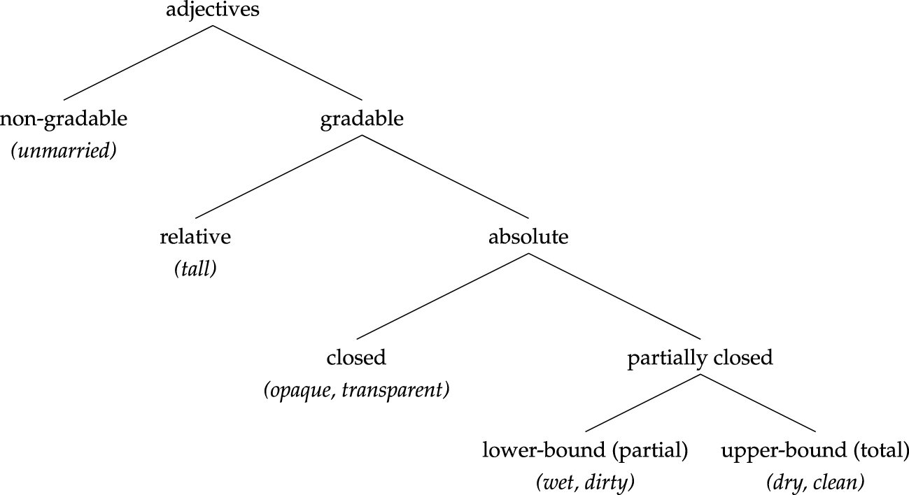
Following Kennedy (Reference Kennedy2007) and Syrett, Kennedy & Lidz (Reference Syrett, Kennedy and Lidz2010), we take the ‘definite description test’ to diagnose the difference between relative and absolute adjectives (see Figure 1 for a schema of these subclasses). In a context in which there are several glasses, all differing in height, a definite description formed with a relative adjective, as in (14a), picks out the individual that instantiates the gradable predicate to the highest degree (i.e. the tallest one), regardless of whether or not the individual counts as tall in the context. In contrast, a definite description formed with an absolute adjective, as in (14b), has a referent only in a context in which a glass actually counts as empty. In a context in which there are several glasses, all containing different levels of liquid (but none empty), (14b) fails to have a referent.

Kennedy’s explanation for this contrast is that relative adjectives, but not absolute adjectives, invoke context-dependent standards.
Within the category of absolute adjectives, there are several subtypes, depicted in Figure 1. These subtypes are differentiated in part by their distribution with a certain class of adjectival modifiers. We will focus on almost and slightly (Rotstein & Winter Reference Rotstein and Winter2004). In a relative antonym pair, neither antonym can be modified by either of these modifiers:Footnote [10]

Adjective classification.

In contrast, in closed absolute antonym pairs, both antonyms can occur with both modifiers:

The partially closed subclass of absolute adjectives differ with respect to which modifier they are compatible with. Total adjectives can be modified by almost but not by slightly and partial adjectives can be modified by slightly but not by almost. (The total/partial distinction is called ‘universal/existential’ in Kamp & Rossdeutscher Reference Kamp and Rossdeutscher1994, Yoon Reference Yoon1996 and Rotstein & Winter Reference Rotstein and Winter2004.)

Beginning with work in Kennedy & McNally (Reference Kennedy and McNally2005), the differences between these classes have been attributed to differences in the structure of the scales with which these adjectives are associated. They propose that absolute adjectives lexicalize bounds on their associated scales, while relative adjectives do not. The difference between total and partial adjectives is thus claimed to be that the former lexicalize an upper bound on the scale (a maximum endpoint) while the latter lexicalize a lower bound on the scale (a minimum endpoint). This claim is bolstered in part by independent evidence that almost selects for scales with upper bounds while slightly selects for scales with lower bounds.
The closed absolute adjectives in (16) are thought to lexicalize both an upper and a lower bound, hence their compatibility with both modifiers. In contrast, because relative adjectives do not encode any bound, they cannot occur with these modifiers, as demonstrated in (15).
2.2.2 Evaluativity and the absolute/relative distinction
Kennedy (Reference Kennedy2007) argues that these lexicalized bounded scales have specific consequences for the phenomenon of evaluativity. In particular, he proposes that if an adjective lexicalizes a scale with a bound, that bound is co-opted as an evaluative standard. If it does not, context values the standard. His Principle of Interpretive Economy (Kennedy Reference Kennedy2007: 36) is reproduced in (19).

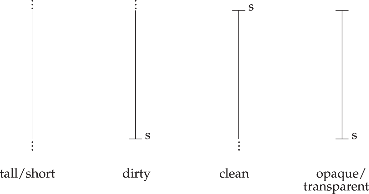
Because relative adjectives contain no conventional meaning that could correspond to a standard, the standards invoked by relative adjectives (but not absolute adjectives) vary from context to context. This is illustrated in Figure 2.
If this is right, there are clear consequences for the study of evaluativity. The distribution of evaluativity reported in Section 2.1 characterizes the behavior of relative adjectives, while the Kennedy/McNally theory predicts that absolute adjectives have a different relationship to the standards by which evaluativity is calculated. In the case of relative adjectives, an individual can be on the scale (say, of tallness) without being above the standard (which could be, say, 6 ft tall). However, the Kennedy/McNally theory predicts that partial adjectives lexicalize a scale with a lower bound, and that this lower bound is co-opted as a standard for the purposes of evaluativity. The result is the prediction that any construction containing a partial adjective will count as evaluative for at least one argument, because any individual that falls on the scale of a partial adjective (e.g. dirty) will necessarily be an individual that exceeds the standard of dirtiness (i.e. the scale’s lower bound). In a comparative formed from a partial adjective, x is Adj-er than y, the subject argument is predicted to be evaluative.
Adjective classes and scale bounds.

In contrast, total adjectives lexicalize a scale with an upper bound, and this bound (given the Principle of Interpretive Economy) is co-opted as a standard for the calculation of evaluativity. As a consequence, any individual on a scale associated with a total adjective is located at or below the standard. The result is that any construction containing a total adjective that differentiates between more than one point on the scale will be non-evaluative for at least one argument.
Closed absolute adjectives like opaque and transparent lexicalize a scale with both an upper and a lower bound. Kennedy’s Principle of Interpretive Economy is silent on which of two bounds should be co-opted for the purpose of evaluativity, and it seems as though the class of closed adjectives is not uniform in this respect. Some closed adjectives (e.g. opaque/transparent) have been characterized as having variable interpretations, in which either bound can function as a standard, while others (e.g. full/empty) seem to only use the maximum standard (Kennedy Reference Kennedy1999).
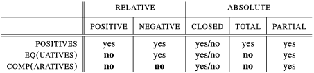
These predictions are largely substantiated by experimental work; see Kennedy & Levin (Reference Kennedy, Levin, McNally and Kennedy2008), Morzycki (Reference Morzycki2009), Syrett et al. (Reference Syrett, Kennedy and Lidz2010), McNally (Reference McNally2011) and Toledo & Sassoon (Reference Toledo and Sassoon2011) for more evidence in support of the Kennedy/McNally theory generally. In particular, while relative adjectives display the evaluativity pattern presented in Section 2.1, partial absolute adjectives are evaluative across constructions and total absolute adjectives are only evaluative in the positive construction, as illustrated in (20)–(23)Footnote [11] and summarized in Table 1. Moreover, there is additional experimental evidence that either bound can function as a standard in degree constructions formed from some closed absolute adjectives (Sassoon Reference Sassoon and Cohen2012a).
Distribution of evaluativity.

However, these judgments, in contrast to the relative adjective judgments, have been reported to be weaker and more controversial; see, in particular, Toledo & Sassoon (Reference Toledo and Sassoon2011), but also Sassoon (Reference Sassoon2012b), for claims that the relative adjective data are more variable than reported here.Footnote [12]

2.3 Theoretical summary
The first goal of the present study is to provide an experimental test for the predictions of the Kennedy/McNally theory, which characterizes different adjective classes in terms of their scale structure, and in particular in terms of which (if any) scalar bounds they lexicalize. If the difference between relative and absolute adjectives is really a difference in scale structure – and, in turn, a difference in the availability of a contextually stable standard of comparison – then we predict that the two classes of adjectives will behave differently in the distribution of evaluativity across degree constructions and across contexts.
The pattern of evaluativity predicted by the Kennedy/McNally theory is generally supported by the introspective judgments provided in the theoretical literature (e.g. Rett Reference Rett, Gibson and Friedman2008a,Reference Rettb; Morzycki Reference Morzycki2009; Syrett et al. Reference Syrett, Kennedy and Lidz2010; McNally Reference McNally2011), but the judgments are regularly reported as relatively weak or variable (see Rett Reference Rett2015 Section 5.4 for an in-depth discussion of this variation).
There are several possible explanations for the variation in these judgments. First, as discussed in Section 2.1, the standard tests for evaluativity are somewhat flawed. The Bierwisch Test and the Negative Antonym Entailment Test only detect evaluativity in clauses that are not embedded under truth-conditional operators. The Bierwisch Test has an additional flaw in that it cannot be applied equally across degree constructions: for positive constructions, the Bierwisch Test amounts to a tautology, a test of whether, e.g., the sentence John is tall entails the sentence John is tall. In other words, the reported judgments of evaluativity could be variable because we are not testing them properly (or consistently, etc.).
Second, speaker intuitions about evaluativity could be variable because evaluativity is context-sensitive. This is certainly true for the evaluativity associated with relative adjectives, but also arguably true for absolute adjectives. Kennedy’s Principle of Interpretive Economy exhorts the speaker to maximize the conventional meanings of a sentence, but an absolute adjective’s lexicalized standard will no doubt vary across comparison classes: as Whorf pointed out (Reference Whorf1956: 135), standards of emptiness seem to vary between bottles of beer and drums of gasoline. Depending on the formal status of Kennedy’s principle, it might be overruled by other considerations in some contexts of utterance but not others.
Third, speaker intuitions about evaluativity could be variable because they are by nature variable; Rett (Reference Rett2015) proposes that evaluativity arises as a conversational implicature, and suggests that variation in evaluativity across antonym pairs could be attributed to the different extents to which evaluativity as an implicature is conventionalized for those antonym pairs based on potential differences in frequency, breadth of meaning, and in the relationship between antonyms in a pair (Lehrer Reference Lehrer1985).
From this perspective, the phenomenon of evaluativity is a compelling area for experimental investigation. Controlled experiments have the potential to contribute consistency and subtlety to the debates outlined above. However, because evaluativity is relatively uncontroversial as a general phenomenon, it is also tempting grounds on which to explore experimental methods of context-sensitive phenomena.
We begin our experimental tests of evaluativity in Section 3 by addressing the extent to which relative and absolute adjectives differ in their evaluativity across degree constructions. The results we report largely confirm the predictions made by the Kennedy/McNally theory, with the exception of one particularly surprising observation: contrary to reports in the linguistic literature, the data suggest that comparatives are evaluative. We further investigate this result in a third experiment, reported in Section 4, which we argue illuminates an important difference in context sensitivity between informal introspective judgments and at least some experimental methodologies.
3 Evaluativity and adjective class
The goal of these experiments is to test the distribution of evaluativity across degree constructions and adjective classes. The experiments share a common methodology: a Bierwisch Test couched in what we call a ‘justifiable entailment task’. Participants were presented with a series of deductions that a Police Chief made based on one-sentence reports from his Detective. The participants were asked to evaluate how justified the Chief’s conclusions were on a five-point Likert scale:
 $-2$
(not justified at all),
 $-1$
(somewhat unjustified),
 $0$
(neither justified nor unjustified),
 $1$
(somewhat justified),
 $2$
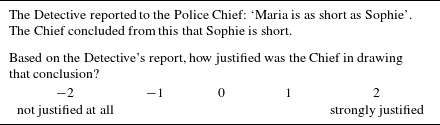
(strongly justified). An example stimulus is provided in Table 2.
All of the stimuli (items or fillers) had the same format; the only parts that changed were the Detective’s quoted report The Detective reported to the Police Chief: ‘…’ and the Chief’s conclusion in the subordinate clause The Chief concluded from this that …. As we will discuss in detail below, the target sentence (in the Detective’s report) changed according to degree construction and adjective class.
Example stimulus.

This methodology uses speakers’ judgments about whether a conclusion is justified as a proxy for entailment in a context of evaluation, which is a discourse variant of the Bierwisch Test.Footnote [13] Because it tests inference from speaker to hearer, the judgments from this design are more context-sensitive than the results of the Bierwisch Test. Presenting the data in a conversation might mean that subjects are more likely to interpret the utterance with some conversational implicature; incorporating a second agent might signal to subjects that two different standards could be at play. In Section 3.2, we will argue that our results suggest that subjects do indeed enrich these sentences with context in a way that the Bierwisch Test does not predict.
A pilot study allowed us to test this methodological approach and confirm that it was a reliable indication of evaluativity. The results of this pilot were replicated by our first main experiment, discussed next, so we will not present the pilot here. See Appendix A for those data and results.
3.1 Method and results
Before turning to the discussion of the experimental method and the results, we briefly recapitulate the predictions made in previous linguistic literature in terms of our expectations for the experiment at hand: (i) we expect the positive construction to be evaluative tout court – in particular, we expect no difference in evaluativity across adjective classes; (ii) we expect to see a difference in evaluativity between positive and negative polarity adjectives in equatives, but not in positive constructions or in comparatives (in either subject or object position); and (iii) we expect to see some differences in evaluativity between relative and some absolute adjectives in comparatives, as detailed in Table 1.
3.1.1 Method
The main goal of Experiments 1 and 2 was to test the difference in evaluativity across the relative and absolute adjectival classes, and with respect to different construction types and adjective polarities. Adjective class was a between-subject variable, i.e. Experiment 1 tested relative adjectives exclusively, while Experiment 2 tested only absolute adjectives. We will continue to distinguish between these two experiments in the discussion of the method, participants and data summaries. When we turn to the statistical analysis, however, we will pool together the data from both experiments and analyze it as one data set. As already indicated, we distinguish between the data collected in Experiment 1 versus Experiment 2 in the statistical analysis by adding an additional factor for adjective class (relative versus absolute adjectives).
Construction type and adjectival polarity were within-subject variables: all combinations were tested in each of the two experiments. The reason for a between-subject design for adjective class is that the experiment (including practice items and a reasonable number of fillers) would have been unfeasibly long.
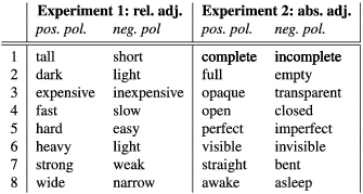
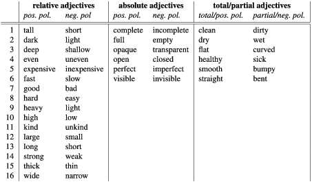
Experiment 1 focused on eight adjective pairs from the relative adjective class, while Experiment 2 focused on eight adjective pairs from the absolute adjective class. These are listed in Table 3 according to their adjectival class.
Experiments 1 and 2: antonym pairs.

The absolute adjective class contains both closed absolute adjectives and total/partial antonym pairs. The first within-subject condition was adjectival polarity. In both adjectival classes, polarity was determined based on the markedness tests developed in Cruse (Reference Cruse1976), Lehrer (Reference Lehrer1985) and Cruse (Reference Cruse1986): the negative antonym in a pair is the more morphologically complex member, and the member with the least natural nominalized form, etc. (cf. openness versus *closedness). For the two total/partial antonym pairs in the absolute condition, the partial antonym was also the negative antonym (cf. straightness versus *bentness, and awakeness versus *asleepness).
The already large number of cells in the present experiments prevented us from investigating the specific predictions made in the Kennedy/McNally theory with respect to the difference in evaluativity between total and partial adjectives. However, we investigated this issue in the pilot experiment discussed in Appendix A. In the pilot, there was no significant difference generally (i.e. across all constructions) between positive and negative antonyms in the relative and closed absolute classes, but there was a significant difference between total and partial antonyms. This difference is still monitored in the present experiment using polarity. In general, in terms of evaluativity across constructions, total adjectives behaved in the pilot like relative adjectives while partial adjectives behaved in the pilot like closed absolute adjectives.
The second within-subjects condition was construction type. We tested for evaluativity in three different constructions: the positive construction, the comparative, and the equative, exemplified in (24).

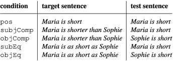
However, for reasons discussed in Section 2.1, we are interested in testing for evaluativity in both clauses of the equative and comparison constructions, so the construction condition has five sub-conditions, illustrated in Table 4.
Sub-conditions of construction type.

Eight items were constructed for each of the posPol-negpol adjective pairs listed in Table 3. That is, Experiment 1 involved a set of 64 items and Experiment 2 involved a distinct set of 64 items. Every item was passed through 10 conditions (2 adjective polarities
 $\times$
5 construction types). Every participant saw each of these items exactly once, with either the posPol or the negPol adjective, and in one of the five construction types, for a total of 64 stimuli (excluding fillers). The adjective polarity & construction type combination was randomly selected for every one of the 64 items and rotated for every participant (Latin square design).
The participants were presented with a series of deductions that a Police Chief made based on one-sentence reports from his Detective. They were asked to evaluate how justified the Chief’s conclusions were on the same five-point Likert scale:
 $-2$
(not justified at all),
 $-1$
(somewhat unjustified),
 $0$
(neither justified nor unjustified),
 $1$
(somewhat justified),
 $2$
(strongly justified) (see Table 2 above). Examples (25) and (26) contain example stimuli in the subjComp condition, (25) from the relative adjective experiment (Experiment 1) and (26) from the absolute adjective experiment (Experiment 2).

In addition to the 64 experimental stimuli, there were 67 fillers involving modal expressions: the modal verb must; the modal verb might; the modal adverb certainly; the modal adverb possibly; the modal/evidential adverb apparently; and the modal/evidential adverb supposedly. The fillers were meant to elicit ratings across the entire range: possibility modal expressions were meant to elicit low ratings, while the ones with necessity modal expressions were meant to elicit higher ratings.Footnote [14] Thus, every participant responded to 131 stimuli (64 experimental stimuli + 67 fillers), the order of which was randomized for every participant.
The sets of participants in the relative and absolute conditions (i.e. in Experiments 1 and 2) were disjoint. Forty-five participants (undergraduate students from UCLA) completed the relative adjective study online on a UCSC-hosted installation of the IBEX platform (http://code.google.com/p/webspr/) for course credit or extra-credit. Sixty-four measurements were collected per participant, for a total of
 $2880$
observations. Fifty different participants (undergraduate students from UCLA) completed the absolute adjective study online on a UCSC-hosted installation of the IBEX platform for course credit or extra-credit. Sixty-four measurements were collected per participant, for a total of
 $3200$
observations.
We examined the pattern of responses that the participants gave for the pos (positive) construction to determine whether participants properly completed the experiment. This construction is the control, as the Bierwisch Test for evaluativity in positive constructions is a test for whether a sentence entails itself, and we expect an overwhelming number of
 $2$
or
 $1$
responses for it from any given participant. If a participant has a consistent pattern of very low responses for the pos construction, e.g.
 $-2$
,
 $-1$
or
 $0$
, relative to the majority of the other participants, it is likely that s/he did not complete the experiment properly and we should drop the data for that participant. We also examined the participants for repeated patterns of behavior that could not be detected by examining consistently low ratings for the pos construction. That is, we checked to see whether any participants selected, e.g., only
 $2$
or
 $1$
throughout the experiment, which would strongly indicate that they did not complete the experiment properly.
As a result, we dropped the data obtained from three participants in Experiment 1 and two participants in Experiment 2. The final number of participants in Experiment 1 was
 $42$
, for a total of
 $2688$
observations, and the final number of participants in Experiment 2 was
 $48$
, for a total of
 $3072$
observations. Aggregating over both the relative and the absolute condition (i.e. over both Experiment 1 and Experiment 2), the final number of participants was
 $90$
and the total number of observations was
 $5760$
.
3.1.2 Results
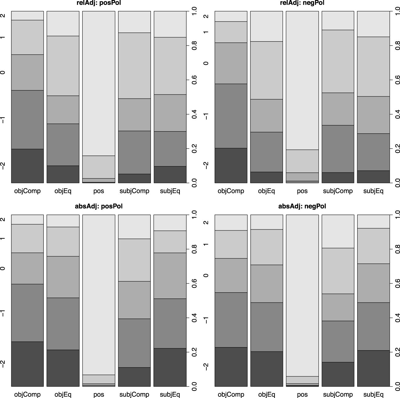
Experiments 1 and 2 – graphical summaries.

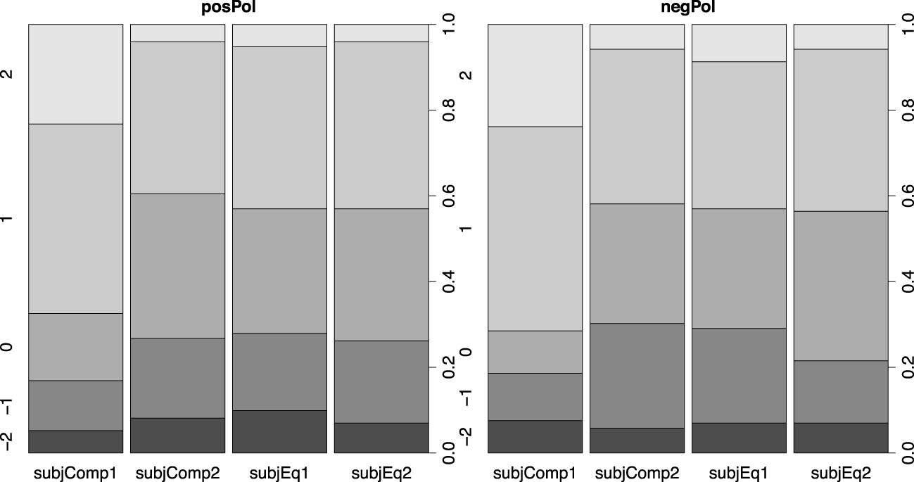
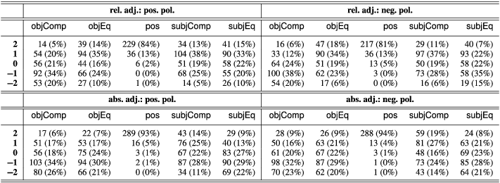
Graphical summaries of the data collected in Experiments 1 and 2 are provided in Figure 3.Footnote [15] There are four plots in this figure. In the first row, we plotted the results for the relative adjective pairs: the plot in the first column from the left corresponds to the positive polarity (posPol) adjectives while the plot in the second column corresponds to the negative polarity (negPol) adjectives. The corresponding plots for the absolute adjective pairs are in the second row; once again, posPol adjectives are in the first column and negPol adjectives in the second. For completeness, the data summaries plotted in Figure 3 are provided in Appendix B.3.
Each plot consists of five equal-width, equal-height bars, i.e. bars whose areas are the same. Each bar corresponds to one of the five constructions under study, listed in alphabetical order on the
 $x$
-axis: objComp, objEq, pos, subjComp, subjEq. Within each bar, we plot the proportion of
 $2$
,
 $1$
,
 $0$
,
 $-1$
, and
 $-2$
answers in increasingly darker shades of gray. Thus,
 $2$
is nearly white and
 $-2$
is nearly black; these values are specified on the
 $y$
-axis on the left side of the plot. Within each bar, the area occupied by a particular shade of gray corresponds to the proportion of times the corresponding number has been selected by participants.
For example, if we focus on the top left plot (relAdj:
posPol), we see that the pos construction has received an overwhelming number of
 $2$
(strongly justified) answers. This is indicated by the very large area that is in the lightest shade of gray. The
 $y$
-axis labels on the right side of each plot help us to infer the actual proportion of
 $2$
answers out of the total number of answers given for the relAdj & posPol & pos condition: we see that this proportion is more than
 $0.8$
, i.e. more than
 $80\%$
. We also see that about
 $0.15$
of the answers were
 $1$
, as indicated by the portion of the bar colored in a slightly darker shade of gray. Finally, there are very few
 $0$
,
 $-1$
or
 $-2$
answers. In contrast, the objComp bar of the same plot indicates that very few
 $2$
or
 $1$
answers have been selected for this construction, since most of the bar is occupied by the areas corresponding to
 $0$
,
 $-1$
, and
 $-2$
.
These plots suggest a set of high-level but richly structured generalizations, taking ‘evaluativity’ as a proxy for ‘acceptability of entailment to the positive construction’.

These generalizations are all underpinned by significant effects, as the data analysis in the following subsection shows. We return to a discussion of these generalizations and their theoretical relevance in Section 3.2.
3.1.3 Statistical analysis: Ordinal probit regression models
The data are not continuous but ordered categorical, i.e. the possible answers
 $-2$
,
 $-1$
,
 $0$
,
 $1$
, and
 $2$
are merely ordered labels rather than actual numbers – in much the same way that the grades
 $A$
,
 $B$
,
 $C$
,
 $D$
, and
 $F$
in the US grading system, or the different levels on a pain or happiness scale, are merely ordered labels.
Our task is to find out whether different adjective classes, different adjective polarities, and different constructions are associated with different levels of evaluativity, while taking seriously the ordered categorical nature of our evaluativity data. To develop a better intuitive understanding of the question we are asking and the way in which we will quantify it, let us restrict our attention to relative adjectives (relAdj) in the positive construction (pos), and simply compare the posPol and negPol conditions, i.e. the positive polarity and the negative polarity adjectives. This is like trying to find out whether the level of scholarly ability of a group of Ohio students, for instance, is ‘significantly’ different from the corresponding level of scholarly ability of a group of Michigan students, as measured by their letter grades on the same standardized test.
One of the standard ways of quantifying the difference between these hypothetical Michigan and Ohio students while being faithful to the categorical nature of the letter grades is to say that the grades give us an imperfect image of the underlying, unobserved continuous scholarly ability of the two groups of students. This scholarly ability, just like weight and height, is assumed to have a normal (Gaussian) distribution. To answer the question of whether Ohio and Michigan students differ in ability, then, we would use their respective grades to estimate the mean/center of the normal distributions underlying their respective scholarly abilities. If the estimated means of the normal distributions are very close to each other, we will conclude that the two groups of students are most likely identical in scholarly ability. If the estimated means are clearly apart, we will conclude that the two groups have different scholarly ability. This type of statistical model is called an ordinal probit model: ‘ordinal’ because we deal with ordered categorical data and ‘probit’ because we assume that the underlying continuous ability has a normal (Gaussian) distribution.
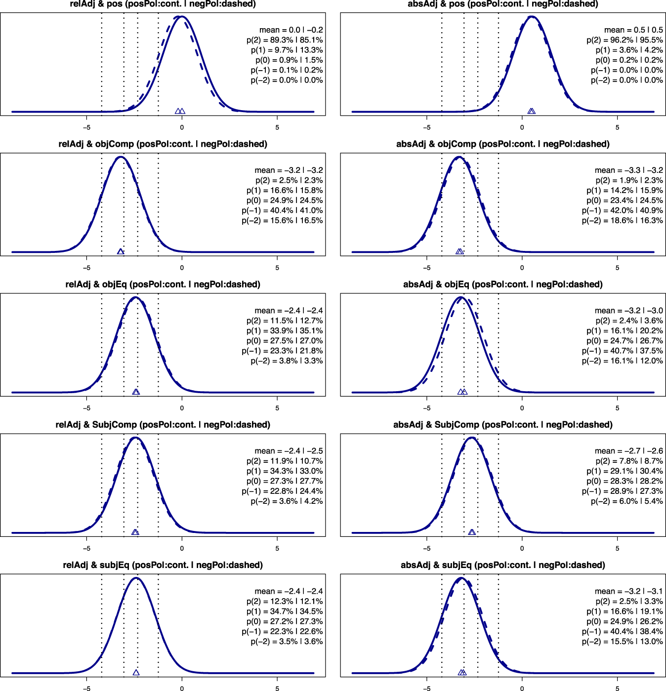
Experiments 1 and 2 – plot of MLEs of the best mixed-effects ordinal probit model. The
 $x$
-axis is the abstract continuous (
 $-\infty$
,
 $+\infty$
) evaluativity scale (only the
 $(-10,10)$
range is plotted). The probability density curve corresponding to posPol is plotted as a continuous line; the density curve corresponding to negPol is plotted as a dashed line. The four vertical dotted lines are thresholds separating the areas under a density curve into five regions: (i) the
 $-2$
region, i.e. the area under the curve that is to the left of the leftmost dotted line; (ii) the
 $-1$
region, i.e. the area between the first and second thresholds; (iii) the
 $0$
region, i.e. the area between the second and third thresholds; (iv) the
 $1$
region, i.e. the area between the third and fourth thresholds; (v) the
 $2$
region, i.e. the area to the right of the fourth (rightmost) threshold. These areas give the probabilities of the five possible outcomes
 $-2$
,
 $-1$
,
 $0$
,
 $1$
, and
 $2$
; they are listed in each plot for both posPol (on the left) and negPol (on the right).

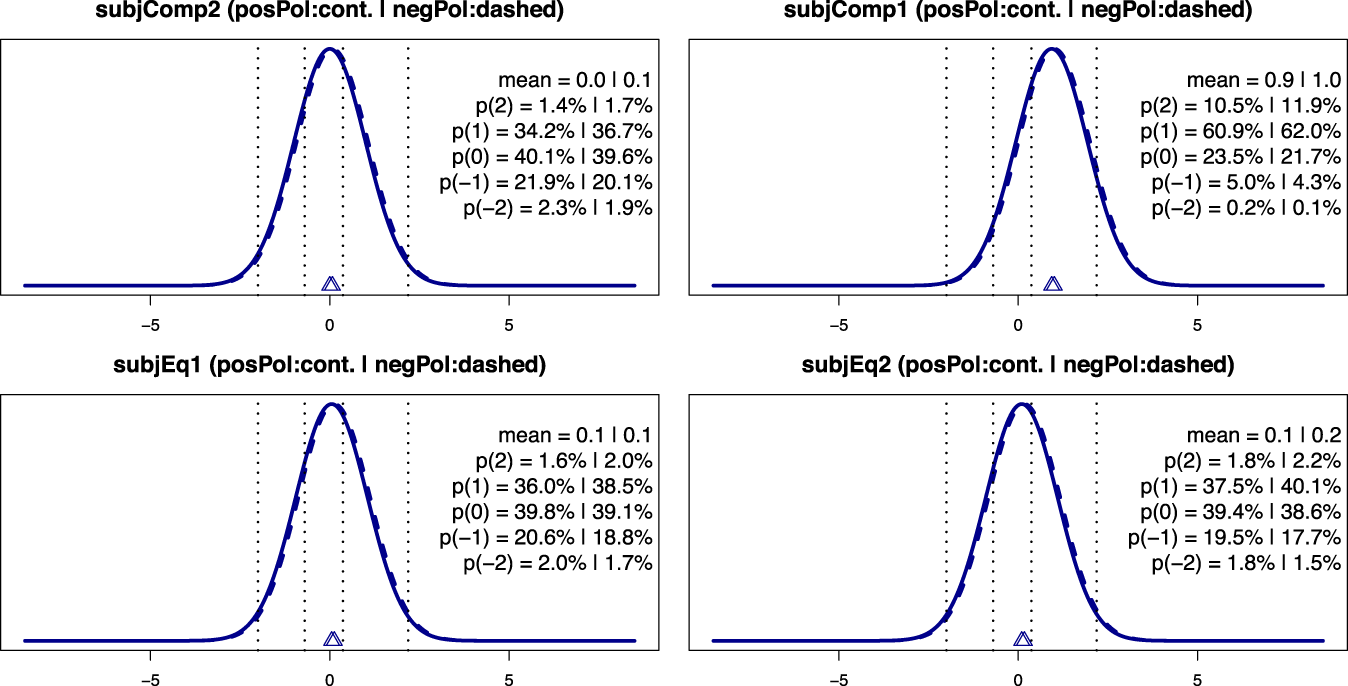
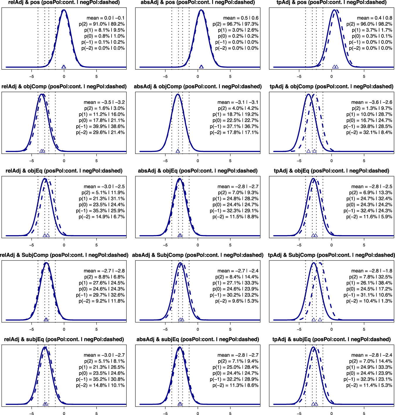
We apply the same statistical model to the results of Experiments 1 and 2, for the same reasons. The estimates are listed in Appendix B.4 and plotted below in Figure 4. Each plot compares two curves corresponding to the probability densities of two different factors. The comparison between the posPol and negPol conditions for relative adjectives (relAdj) in the positive construction (pos) is plotted in the top leftmost plot of Figure 4. The comparison between the posPol and negPol conditions is similar to the hypothetical comparison between Michigan and Ohio students outlined above. On the
 $x$
-axis, we plot the abstract continuous (
 $-\infty$
,
 $+\infty$
) evaluativity scale. The probability density curve corresponding to the posPol condition is plotted as a continuous line while the density curve corresponding to the negPol condition is plotted as a dashed line. The means of the two distributions are
 $0$
and
 $-0.2$
, as listed in the plot. The two triangles on the
 $x$
-axis indicate where these means are located: we see that the two triangles are basically on top of each other, indicating that the posPol and negPol conditions are not really distinct. This means that, in Experiment 1, subjects did not treat sentences like John is short and sentences like John is tall as different with respect to their evaluativity.
The four vertical dotted lines in the plot are the thresholds separating the area under a density curve into five regions: (i) a
 $-2$
region, which is the area under the curve that is to the left of the first threshold, i.e. to the left of the leftmost dotted line; (ii) the
 $-1$
region, which is the area under the curve between the first threshold and the second threshold; (iii) the
 $0$
region, which is the area under the curve between the second and the third thresholds; (iv) the
 $1$
region, which is the area under the curve between the third and the fourth thresholds; and finally (v) the
 $2$
region, which is the area under the curve to the right of the fourth (rightmost) threshold.
Figure 4 provides plots for both adjective classes – relAdj in the first column, absAdj in the second column – and for all five construction types – pos in the first row, objComp in the second row, objEq in the third row, subjComp in the fourth row, and finally subjEq in the fifth row. It should be noted that the thresholds (the dotted vertical lines) are in the exact same places in all of the plots: their placement is estimated based on the whole data set and their positions are the ones that fit/account for the data the best.
Once estimated, the thresholds are fixed, so probabilities, i.e. the areas of the five regions under a curve, can vary only if the mean/center of the curve (represented as a triangle in Figure 4) moves to the left or to the right. The further to the right a density curve is, the more evaluative the corresponding condition is. This is because moving a curve to the right increases the area of the rightmost regions, i.e. the probability of getting a
 $2$
or a
 $1$
answer. The further to the left a density curve is, the less evaluative the corresponding condition is. This is because moving a curve to the left increases the area of the leftmost regions, i.e. the probability of getting a
 $-2$
or a
 $-1$
.
As listed in the top leftmost plot in Figure 4, the probability of getting an answer of
 $2$
for a positive construction with a positive antonym in the relative adjective condition is very high, namely
 $89.3\%$
; this is because region
 $2$
(the region to the right of the rightmost threshold) covers most of the area under the continuous (posPol) curve. The dashed (negPol) curve is slightly displaced to the left because its mean is
 $-0.2$
, so its corresponding region
 $2$
covers slightly less of the full area – only
 $85.1\%$
. Thus, the probability of getting an answer of
 $2$
for the negPol condition is
 $85.1\%$
, which is slightly less than the corresponding probability of
 $89.3\%$
for the posPol condition.
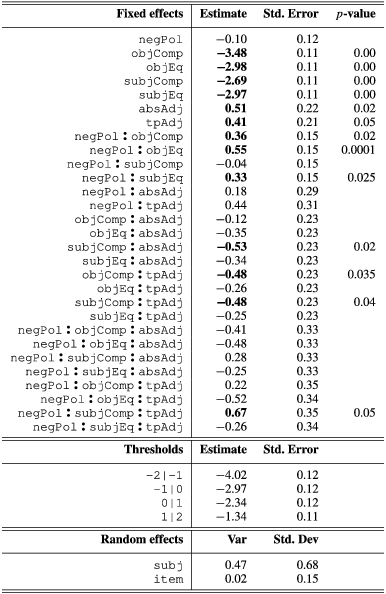
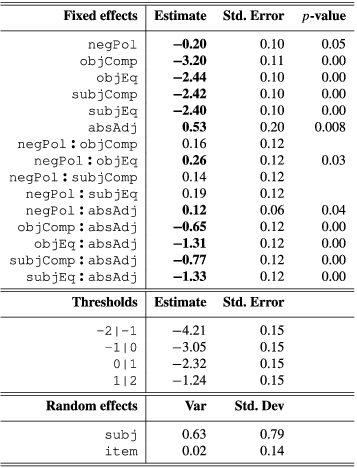
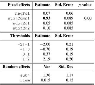
Technically speaking, the model whose maximum likelihood estimates (MLEs) are plotted in Figure 4 is a mixed-effects ordinal probit regression model, with fixed effects for adjective class, construction type, adjective polarity, and all of their two-way interactions (but not the three-way interaction between adjective polarity, adjective class, and construction type), and intercept random effects for subjects and items. Likelihood ratio tests (LRTs) determined this to be the best model, i.e. the model that strikes the best balance between complexity (number of estimated parameters) and data fit. As we have already indicated, the MLEs, their standard errors and corresponding
 $p$
-values (if less than
 $0.05$
) are provided in Appendix B.4; these estimates provide support for the generalizations we listed in (27). The same appendix also provides more details about the LRTs we conducted. Finally, to intuitively see how closely the model fits the data, we encourage the reader to compare the estimated (model-based) probabilities provided in Figure 4 and the corresponding empirical probabilities listed in Appendix B.3.
Analyzing evaluativity in terms of ordinal probit models assumes that the ordered categorical responses provide an imperfect image of an underlying continuous evaluativity dimension in the same way that grades provide an imperfect image of an underlying continuous scholarly ability. If this seems undesirable, the reader is encouraged to think of the underlying continuous probability distribution as a mathematical tool that enables us to statistically analyze our data while respecting its ordered categorical nature – in much the same way that we can think of possible-world semantics as a tool to analyze intensional phenomena in natural language without necessarily attributing psychological reality to possible worlds.
3.2 Discussion
The generalizations presented in Section 3.1.2 (see (27)) are supported by the ordinal probit model above. In what follows, we discuss these results and their theoretical consequences. We begin in Section 3.2.1 by discussing the (perhaps surprising) lack of a polarity effect. In Section 3.2.2, we discuss the unsurprising strong evaluativity of the positive construction, and in Section 3.2.3, we discuss the relative/absolute distinction that was the focus of this study. We end by discussing the comparison construction effects, which form the basis for Experiment 3.
3.2.1 The lack of a polarity effect
It should be recalled that relative antonyms are reported to differ in their evaluativity in a complicated way (see Table 1 in Section 2.2.2). An adjective and its antonym are reported to pattern together with respect to evaluativity in two out of three tested degree constructions: the positive construction (where both antonyms are evaluative) and the comparative construction (where neither antonym is evaluative). An antonym and its adjective are expected to contrast in evaluativity only in the equative construction.
The first generalization reported above for Experiments 1 and 2 is that there is no main effect of adjectival polarity, for either the relative or absolute adjective pairs. We see a borderline significant main effect of polarity for relative adjectives in the positive construction (i.e. in the Experiment 1 data), but it goes in the unexpected direction: negative polarity antonyms seem to be less evaluative than their positive polarity counterparts. However, because this effect is only borderline significant (the
 $p$
-value is close to but slightly larger than
 $0.05$
; see Appendix B.4), and no such effect was observed in the pilot experiment (see Appendix A), we will conservatively take this effect to be noise and will not discuss it further.
The lack of a polarity effect is consistent with the across-the-board intuitions reported in Table 1 (with equative constructions being the sole exception). Numerically, we see that this contrast is reflected in our Experiment 2 data (i.e. for absolute adjectives) – see the slight displacement to the right of the dashed density curves in the absAdj & objEq and absAdj & subjEq plots in Figure 4. However, this provides almost no evidence for or against the contrast reported in the theoretical literature. Follow-up experiments focused on polarity contrasts in equative and (possibly separately) positive constructions are needed before we can decide whether our experimental task was not discriminating enough to detect the effect or whether there is actually no effect.
3.2.2 The strength of evaluativity across constructions
For both relative and absolute adjectives, the positive construction tested as significantly more evaluative than the other constructions. One way to quantify this is to look at how probable it is to receive a rating of
 $2$
or
 $1$
. For the positive construction, if we sum over
 $p(2)$
and
 $p(1)$
, we get very close to
 $100\%$
probability, i.e. the positive construction is basically certain to receive a rating of
 $2$
or
 $1$
.Footnote
[16]
For all of the other constructions, this probability is much lower: it never exceeds
 $20\%$
for objComp and it is at most in the high
 $40\%$
s for the other three constructions. The overwhelming strength of the effect for the positive construction makes it more difficult to compare the potential evaluativity of the more complex comparison constructions.
There are a few plausible explanations for the strength of this effect. It is possible, as is traditionally assumed, that only the positive construction is evaluative (Bartsch & Vennemann Reference Bartsch and Vennemann1972, Cresswell Reference Cresswell and Partee1976, Kennedy Reference Kennedy1999), and the perceived evaluativity of any other construction is insignificant or mistaken. Our statistical analysis does not present strong evidence against this claim but suggests that other adjectival constructions are somewhat evaluative and subjects are sensitive to differences in evaluativity exhibited by these other constructions.
However, if we take seriously the hypothesis that non-positive constructions are to some extent evaluative, how can we explain the large asymmetry in evaluativity between these constructions and the positive one? In particular, in view of the previous linguistic literature, we expected equative constructions (at least with negative polarity adjectives) to be basically as evaluative as the positive construction.
One possible explanation for the much stronger evaluativity of the positive construction is that its evaluativity is at-issue/truth-conditional while the evaluativity for the other constructions is presupposed/not at-issue. It is possible that the Bierwisch Test primarily targets at-issue evaluativity, and cooperative experimental subjects – who are sensitive to the distinction between asserted and presupposed content – respond accordingly.
An alternative explanation is that the strength of evaluativity for positive constructions is the result of the particular methodology employed here: positive constructions trivially pass the Bierwisch Test (the Bierwisch Test amounts to a test of whether
 $p\Rightarrow p$
) while other constructions can only pass the test non-trivially. Thus, it is possible that the strength of the effect of evaluativity in the positive construction is an artifact of this methodological asymmetry.
However, we see a significant difference between relative and absolute adjectives in the positive construction: absolute positive constructions are more evaluative than relative positive constructions – see Figure 4 above, where the absAdj means for the pos construction are about
 $0.5$
while the means for relAdj & pos are
 $0$
or thereabouts. This makes the methodological asymmetry explanation (on its own) unlikely: the fact that there is a significant difference between absAdj and relAdj indicates that subjects were not treating the Bierwisch Test as a trivial inference in the case of the positive construction; instead, the contrast between absolute and relative adjectives reflects independently observed differences between the types of standards employed by the two types of adjectives (Rotstein & Winter Reference Rotstein and Winter2004, Kennedy & McNally Reference Kennedy and McNally2005).
3.2.3 The relative/absolute distinction
The Kennedy/McNally theory is that relative and absolute adjectives differ with respect to the structure of the scale they are associated with. In particular, that the scales associated with relative adjectives (tallness, heaviness) are unbounded while the scales associated with absolute adjectives (opacity, transparency) are bounded, intrinsically, at one or more ends of the scale.
In part based on these observations, and in part based on an investigation of the interaction between these adjectival classes and vagueness, Kennedy (Reference Kennedy2007) argues that relative adjectives invoke contextually valued standards, while the standards invoked by absolute adjectives are their lexicalized bounds. This is his Principle of Interpretive Economy (19). Because relative adjectives have no conventional meaning that could correspond to a standard, the standards invoked by relative adjectives (but not absolute adjectives) vary from context to context. If this is right, then an account of the experimental results that emphasizes the role of context (or a lack of context) predicts that relative and absolute adjectives will behave differently. This is in fact what we see.
In the positive construction condition, in which subjects were asked whether
 $p\Rightarrow p$
, the entailment pattern between positive constructions with absolute adjectives was judged to be more acceptable than the entailment pattern between positive constructions with relative adjectives (
 $\unicode[STIX]{x1D6FD}=0.53,\text{SE}=0.20,p=0.008$
– see the main effect for absAdj in the model estimates reported in Appendix B.4). That is, subjects were more likely to assent to (28a) than (28b).

The raw data are as follows: for relAdj&posPol,
 $84\%$
of the ratings were
 $2$
and
 $13\%$
of the ratings were
 $1$
, while for absAdj&posPol,
 $93\%$
of the ratings were
 $2$
and
 $5\%$
of the ratings were
 $1$
(for more information, including the actual counts, see the table in Appendix B.3). This is a remarkable result if subjects are treating the positive construction only as an instance of trivial entailment.Footnote
[17]
The putative difference between relative and absolute adjectives in terms of their context sensitivity can help to explain the difference, though: because the standards invoked by absolute adjectives are just their bounds, absolute positive constructions are not context-sensitive in the way that relative ones are. That is, if it is the case that Bert’s book is complete in one context, it is complete in all contexts. However, this is not necessarily the case if Helen’s book is good.
This strongly suggests that subjects are aware of contextual sensitivity in these constructions, and that they are less likely to accept the Bierwisch Test in the case of a contextually sensitive positive construction than they are in the case of a contextually insensitive construction. Importantly, it also suggests that subjects are considering contextual variability when they are asked about the reliability of a sentence’s entailment, even when their judgments are elicited with respect to a specific context.
Other constructions also show evidence of a difference between relative and absolute adjectives. While subjects did not treat relative and absolute adjectives differently in comparatives, they did treat them differently in equatives: equatives with relative adjectives were judged to be more evaluative than equatives with absolute adjectives. This means that the entailment pattern exemplified in (29a) was judged as significantly more acceptable than the entailment pattern exemplified in (29b), for both subjects and objects of equatives.

One should recall from Section 2.1 a reported asymmetry between the subjects and objects of equatives: projection tests determined that the evaluativity presupposed by equative constructions seemed to be associated with the objects, but not the subjects, of equatives. Despite this asymmetry, the truth conditions of an equative equate one height with another, which effectively transfers the evaluativity of one individual to the other individual. This is confirmed by the near equality of the subjEq and objEq conditions.
In sum, subjects clearly differentiated between relative and absolute adjectives, but they did so in a complicated way. They treated absolute adjectives as significantly more evaluative in positive constructions, but relative adjectives as significantly more evaluative in equatives. And they did not differentiate between relative and absolute adjectives in comparatives. It seems plausible that this result evaded prior notice because, unlike reports of speaker’s intuitions about evaluativity, the current experimental task was both fine-grained and precise enough to determine whether two evaluative constructions differ in their degree of evaluativity (or the degree to which speakers feel comfortable characterizing evaluativity as a reliable entailment of a construction across contexts).
It is not clear how to reconcile these two differences between relative and absolute adjectives. One prominent difference between positive constructions and equatives is that the former involve one individual and its measure, while the latter involve two individuals and their measures. The Kennedy/McNally theory predicts a positive construction formed with an absolute adjective to be evaluative because the standard of comparison invoked is the adjective’s maximum. However, it is possible that the introduction of two relevant individuals makes the interpretation of an absolute-adjective equative more vulnerable to contextual considerations, thereby weakening the relationship between the absolute adjective’s maximum and evaluativity in the context of evaluation.
In particular, it might be that in the case of absolute adjectives, there is a (pragmatic) competition between two different equative strategies, the coordination strategy in (30a) (Haspelmath & Buchholz Reference Haspelmath, Buchholz and van der Auwera1998) and the familiar degree-quantifier strategy in (30b).

While (30a) equates individuals with respect to an absolute property, the degree-quantifier strategy in (30b) equates degrees of emptiness. In the case of absolute properties (and thereby maximal standards), the choice between these two constructions might bear on the evaluativity of the sentence: an utterance of (30b) might be taken to implicate that the maximum standard is not met in the context of interpretation.
In conclusion, it is clear that subjects calculate evaluativity differently for relative and absolute adjectives. In the case of positive constructions, which are overwhelmingly judged to be evaluative, they seem to do so in a way that is predicted by the Kennedy/McNally approach: positive constructions formed with absolute adjectives are even more likely than those formed with relative adjectives to be judged as evaluative. This is presumably because the evaluativity of these constructions is conventionalized or lexicalized in a way that it is not for relative adjectives. However, the (less evaluative) equative constructions displayed the opposite trend. While we have only speculated about this potential difference between positive constructions and equatives, these curiosities about the role of context in this experiment and in the calculation of evaluativity generally – as well as the result about comparative constructions discussed immediately below in Section 3.2.4 – form the basis for Experiment 3, discussed in Section 4.
3.2.4 Evaluativity in comparison constructions
This section discusses one final major result of Experiments 1 and 2. Despite the dwarfing effect of the positive construction, there is still reason to think that subjects treated the two comparison constructions – comparatives and equatives – as evaluative, at least to some extent.
Across adjective types, participants judged the subject position of a comparative to be more evaluative than the object position (or the subject/object positions in equatives). Specifically, the subject position of comparatives entails the corresponding positive construction to a significantly larger extent than the object position of comparatives:
 $p(2)+p(1)$
is around
 $40\%$
for subjComp and less than
 $20\%$
for objComp. This means that subjects were significantly more likely to accept the entailment in (31a) than the one in (31b) (or the entailments for either argument of the equative).

This result is in direct conflict with intuitions reported in the theoretical literature, illustrated in (32) (and discussed in Section 2.1).

However, interestingly, this result is consistent with some preliminary experimental investigations of evaluativity in the psychology and experimental linguistics literature. Psychologists interested in deductive reasoning as a cognitive process in children and adults have tested the processing and interpretation of comparatives (Piaget Reference Piaget1928; Donaldson Reference Donaldson1963; Clark Reference Clark1969a,Reference Clarkb; Flores D’Arcais Reference Flores D’Arcais, Flores D’Arcais and Levelt1970; Clark Reference Clark1972; Higgins Reference Higgins1977). For example, although Clark’s focus was on the speed at which the subjects correctly deduced transitive relationships encoded in multiple comparative constructions, he also tested for evaluativity (which he referred to as ‘contrastiveness’), focusing almost exclusively on better and worse comparatives.Footnote [18]
Clark observed that for a comparative of the form ‘
 $A$
is
 $P$
-er than
 $B$
’, subjects are likely to conclude that
 $A$
is
 $P$
, but not that
 $B$
is
 $P$
(p. 397). In other words, subjects are more likely to interpret a comparative as characterizing the external argument as evaluative. This claim is strengthened by work in Flores D’Arcais (Reference Flores D’Arcais, Flores D’Arcais and Levelt1970) (who argues that this ‘positional asymmetry’ is restricted to comparatives formed with positive antonyms). The result seems to be especially clear in the testing of children. Clark reports an earlier study conducted by Piaget, in which children were presented with the following problem:

Piaget’s description of their responses is as follows.

Even more striking, the evaluativity in comparatives is so compelling that when the children were presented with a series of comparatives that differed in polarity, they were forced to contradictory conclusions.

This sort of error is apparently very frequent: it accounts for about 70% of errors in Donaldson’s study.
In contrast, Higgins (Reference Higgins1977) observed no difference in evaluativity between the subject and object position. (Like the others, he did not test for evaluativity in any other adjectival construction, although he did expand his stimuli to include relative and extreme adjectives, like obese.) However, his method departs from the Bierwisch Test: instead of asking about the meaning of a sentence, he asks about its acceptability (whether it ‘sounds right’) in contexts in which the evaluativity is implausible, e.g. for sentences like A feather is heavier than a snowflake. In every case, judgments of acceptability relied on the subjects’ world knowledge in addition to their linguistic knowledge. It therefore seems reasonable to attribute the contrast between his results and those of the others to the fact that the others used some version of the Bierwisch Test, while Higgins tested for evaluativity by seeing which constructions were (in)compatible with contextually insensitive real world knowledge of evaluative properties.
Getting back to the present study: the results of Experiments 1 and 2 suggest that participants consider the subjects of comparatives to be evaluative, in contrast to the objects of comparatives and even to (either argument of) equative constructions. These results directly contradict intuitions reported in the linguistics literature and run up against theories designed to predict those intuitions.Footnote [19] They do, however, seem to replicate some limited previous experiments in the psychology literature – in particular those in Piaget (Reference Piaget1928), Clark (Reference Clark1969a,Reference Clarkb), Flores D’Arcais (Reference Flores D’Arcais, Flores D’Arcais and Levelt1970), and Clark (Reference Clark1972) – but arguably only those running some experimental variant of the Bierwisch Test.
What accounts for this surprising result? On one hand, it is possible that the reported intuitions – although widespread – are mistaken. On the other hand, it is possible that the Bierwisch Test, at least in the context of the comparative construction, does not appropriately target evaluativity. In what follows, we present a hypothesis along the lines of this second possibility; in particular, that participants in Experiments 1 and 2 judged the subjects of comparatives to be evaluative because they interpreted comparatives – but not equatives – as creating a context in which the most salient contextual standard is the measure of the individual denoted by the object. Subjects necessarily exceed this measure in comparatives (which encode the
 ${>}$
relation), but not in equatives (which encode the
 ${\geqslant}$
relation). Accordingly, the subject positions of comparatives are judged to be evaluative, but with respect to the object argument, not some other contextual standard. Experiment 3 was designed to directly test this hypothesis, which we expand upon below.
Our hypothesis is in a way expected given the analysis of adjectival vagueness in Barker (Reference Barker2002) as a set of contextual restrictions on degree variables, which is incrementally updated in discourse. He argues that in addition to having presuppositional and assertive content, these ‘vague’ constructions carry a third type of entailment – sharpening – which he defines as ‘what happens to the status of vague predicates as discourse constrains possible ways of resolving that vagueness’ (p. 4; see also Kamp Reference Kamp and Keenan1975, Klein Reference Klein1980, Pinkal Reference Pinkal, Bartsch, van Benthem and van Emde Boas1989). The sharpening components of a construction can also be thought of as metalinguistic meaning.
For example, in a context in which it is clear what the relevant standards of tallness are, the positive construction John is tall carries descriptive meaning; it counts as contributing information about John’s height. In contrast, Barker describes a context in which Feynman’s height is clear, but an interlocutor is interested in knowing what counts as tall in the U.S. In such a context, the positive construction – by virtue of being evaluative – has a metalinguistic contribution; it carries information about the relevant standard of tallness, rather than Feynman’s height. As Barker says:

As Barker presents it, an evaluative construction (or, more generally, a context-sensitive construction) is descriptive in a context in which the contextual standard is known, but metalinguistic or sharpening in a context in which the contextual standard is unknown.Footnote [20]
This dichotomy seems to be relevant for reconciling the intuitions reported in the theoretical literature – that the comparative is not evaluative while the equative is – with the experimental results presented here and in the prior psychology literature that the subject of the comparative is evaluative.
In the theoretical literature, evaluativity judgments are often reported in a particular context; in Section 2.1, we presented them in a context in which John is either extremely tall or extremely short. In experimental studies, on the other hand, evaluativity judgments are extracted in the absence of any contextual information that could inform the speaker about the relevant standard of, e.g., tallness. In the absence of any other information about the context of evaluation, the subject can only infer from the comparative in (31) that (i) the context of evaluation contains two individuals, John and Bill; (ii) those individuals are strictly ordered with respect to their height; and (iii) John’s height exceeds Bill’s height. The Bierwisch Test relies on the participants’ ability to reason about the meaning of sentences across contexts, but it is possible that subjects instead treated this minimal context as the only relevant context of evaluation. Moreover, it seems plausible that in a world in which there are only two individuals, and those individuals are strictly ordered with respect to height, one individual will count as tall, and the other one as not tall (see van Rooij Reference van Rooij, Egré and Klinedinst2011).
In contrast, equatives do not strictly order individuals with respect to a dimension of measurement. Therefore, if the above ‘sharpening’ hypothesis is correct – that is, if subjects are treating the object of comparatives as the relevant standard in the context of interpretation – we also expect that equatives should not exhibit a positional asymmetry with respect to evaluativity since equatives do not strictly order their two individuals. This is in fact what we see: within each of the two relAdj and absAdj classes, subjEq and objEq constructions are very similar.
It is then possible that a comparative uttered in a context with a clear standard is not evaluative (its descriptive use), while a comparative uttered in a context with no clear ‘prevailing standard’ is (its metalinguistic use). In the latter context, implicit comparatives like the degree comparatives studied here would function more like explicit comparatives ((34a), discussed in Kennedy Reference Kennedy2009, Sawada Reference Sawada2009, Kubota & Matsui Reference Kubota, Matsui, Li and Lutz2010) or conjoined comparatives ((34b), discussed in Stassen Reference Stassen1985).

In fact, as a reviewer points out, there is independent experimental evidence that subjects are willing to partition ad hoc comparison classes for the purpose of interpreting evaluative constructions in the absence of explicit information about the standard. Syrett et al. (Reference Syrett, Kennedy and Lidz2010) demonstrates this for children’s and adults’ interpretation of positive constructions; Tribushinina (Reference Tribushinina2011) and Tribushinina & Gillis (Reference Tribushinina and Gillis2012) demonstrate the same for children’s use of degree modifiers. The present study can be taken as evidence that this process is at work outside of evaluative constructions: a variety of degree constructions are interpreted as informing subjects about the nature of the comparison class and, in so doing, the nature of the relevant standard of comparison.
It is important to note that Barker (Reference Barker2002) expressly assumes that degree comparatives are not evaluative, even in the sense we are suggesting, and Kennedy (Reference Kennedy2009), Sawada (Reference Sawada2009), and Kubota & Matsui (Reference Kubota, Matsui, Li and Lutz2010) all consider evaluativity to be a characteristic difference between explicit (degree) comparatives (which allegedly lack it) and implicit comparatives like (34a) (which are evaluative for the subject, John in this case).
Experiment 3, to which we turn in the next section, is designed to test the extent to which the ‘sharpening’ hypothesis is a plausible explanation of the discrepancy between the traditional description of evaluativity in the theoretical literature and our experimental results (or the experimental results in the psycholinguistic literature). If Experiment 3 supports our sharpening hypothesis, it seems that the traditional description of evaluativity is not exactly right/is lacking in nuance. In particular, evaluativity might be detectable in contexts of evaluation with no clearly defined standard (like comparatives) if our measurement procedure is sensitive enough, i.e. not exclusively based on introspective judgments.
3.3 Interim summary
Experiments 1 and 2 comprise a comprehensive study of evaluativity across representative degree constructions and adjective classes. The experimental method employed here is an adaptation of the Bierwisch Test: a Detective utters a degree construction (e.g. Martha is as strong as Bertha) and asks participants to rank on a five-point Likert scale how justified his interlocutor is in concluding that a corresponding positive construction (e.g. Bertha is strong) is true.
While this test amounted to something that looked like a trivial entailment in the case of the positive construction – i.e. a judgment about whether
 $p$
entails
 $p$
– our results in this condition varied significantly across adjective class, suggesting that participants may have relied heavily on contextual cues to differentiate between different uses of the same construction within a single context. This is one of several ways in which Experiments 1 and 2 revealed significant considerations of context in participants’ judgments of the entailments of an utterance.
In addition to illuminating the role of context in judgments of evaluativity, the experimental design added a level of nuance to the study of evaluativity not present in theoretical reports of speaker intuition: its introduction of a Likert scale into the Bierwisch Test allowed for participants to report graded notions of evaluativity. The result is a study of evaluativity that is not categorical (although this does not entail that we need a notion of evaluativity that is not categorical; Hansen & Chemla Reference Hansen and Chemla2013). These gradable responses are particularly useful in comparing the behavior of different adjectival classes within a particular construction – like the positive construction – that has been claimed to be evaluative regardless of adjective type. It also has the potential to better reflect different types or sources of evaluativity. In particular, we were additionally interested in examining the distribution of evaluativity across degree constructions (in particular, comparatives and equatives) and across adjective classes (in particular, relative and absolute adjectives).
With respect to the relative/absolute distinction, the experiment produced two interesting results: first, that participants judged absolute-adjective positive constructions to be significantly more evaluative than relative-adjective positive constructions; and second, that they judged relative-adjective equatives to be significantly more evaluative than absolute-adjective equatives. While the proposal in Kennedy & McNally (Reference Kennedy and McNally2005) predicts these classes of adjectives to behave differently with respect to evaluativity, we know of no theory that predicts a construction-specific difference.
Perhaps the most striking result of Experiments 1 and 2 is the relative evaluativity of the subject position of comparative constructions. In the linguistics literature, both positions of the equative are reported to be evaluative, in contrast to the comparative where neither position is claimed to be evaluative. However, in our experiments, the subject of the comparative was judged to be more evaluative than either argument of the equative, which in turn were judged to be more evaluative than the object of the comparative.
While this result does not seem to be compatible with the intuitions reported in the theoretical literature, it is consistent with some early experiments in the psycholinguistic literature (in particular, those that employ some version of the Bierwisch Test). In Section 3.2.4, we hypothesized that this unexpected result is the consequence of an unforeseen interference of the null context in which the stimulus was presented. In particular, that participants used the comparative (but not the equative) to determine the relevant standard of evaluation. A context consisting only of two strictly ordered individuals is quite naturally divided into a positive and negative extension (the subject and object, respectively), while a context consisting of only two non-strictly ordered individuals is not so naturally divided.
If this is right, it seems as though we have reason to differentiate between two types of evaluativity that can be associated with a given construction: evaluativity that is intrinsic to the construction (part of its descriptive content, either at-issue or not-at-issue) and evaluativity that arises in particular contexts as the result of the construction’s descriptive content plus contextual considerations. The former is the traditional notion of evaluativity while the latter looks somewhat like what Barker (Reference Barker2002) referred to as the metalinguistic use of evaluative constructions. The evaluativity conferred on the subject of a comparative is like Barker’s metalinguistic use of positive constructions in that it serves to value the standard of comparison. It is, however, unlike metalinguistic uses of positive constructions in that comparatives, in contrast to positive constructions, are generally not considered to be evaluative in other contexts.
This is therefore an interesting result in a number of respects. If our explanation is correct, the apparent evaluativity of the subject position of comparatives has the potential to shed light on how context-sensitive expressions are valued and restricted (in Barker’s words, sharpened) from context to context. In addition to informing the study of evaluativity, a better understanding of the interpretation of context-sensitive expressions could be extended to other context-sensitive phenomena as well as models of discourse and context update.
4 Evaluativity and context sensitivity
In this section, we report the results of an experiment explicitly designed to test the hypothesis presented above, namely that the reported evaluativity of the subject of comparatives is the result of the effect the comparative has on shaping/sharpening the relevant context of evaluation (rather than the evaluativity intrinsic to this construction). Experiment 3 is a version of Experiments 1 and 2 in which three rather than two individuals are introduced, and there is a strict ordering between these three individuals. We conclude in Section 5 by discussing the broader implications of this entire series of experiments and directions for future work.
4.1 Method
The main goal of Experiment 3 was to test whether the evaluativity of comparative constructions is sensitive to the context implicitly set up by the comparative in a way that equative constructions are not. In particular, we wanted to test two competing hypotheses about the evaluativity associated with the subject of the comparative in Experiments 1 and 2: (i) subjects of comparatives were considered evaluative because the subject position of comparatives is intrinsically evaluative, like the positive construction; or (ii) subjects of comparatives were considered evaluative because of a contextual effect of the comparison class implicitly set up by the comparative, namely two entities strictly ordered with respect to the scale contributed by the adjective, the higher of which must per force count as exceeding the contextual standard. To test these competing hypotheses, we added a second comparison construction to the stimuli, as in (35).

While Experiments 1 and 2 tested evaluativity in the subject and object positions of a single comparison construction, Experiment 3 tested evaluativity in the subject positions of each of the two conjoined comparison constructions: (35a) shows an example that tests the subject of the first comparative, while (35b) shows an example that tests the subject of the second comparative (which in every case was also the object of the first comparative).
The first hypothesis (evaluativity is intrinsic to the subject position of comparatives) predicts that there should be no difference between the evaluativity of (35a) and the evaluativity of (35b) above, modulo the discourse effects (if any) associated with the fact that the subject in (35a) linearly precedes the subject in (35b). In contrast, the second hypothesis (evaluativity due to the implicitly constructed comparison class) predicts that only (35a), but not (35b), should exhibit clear evaluativity effects.
To factor out the presumed effects of linear precedence, and to have a general baseline against which to assess the evaluativity of subjects in comparatives, we also presented participants with equatives in the same kind of three-entity contexts.

We expect to see no difference between (36a) and (36b) under either of our two hypotheses since the presence of a strict ordering of the kind induced by comparatives but not equatives is a necessary precondition for both hypotheses.
Since the effect of subjComp relative to objComp was most clearly visible for relative adjectives, Experiment 3 focuses only on this adjectival class. Experiment 3 stimuli were formed with basically the same relative adjectives and types of entities as the Experiment 1 stimuli.
Each of the 32 items was passed through eight conditions: two adjective polarities (posPol, negPol)
 $\times$
four construction types (subjComp1 (35a), subjComp2 (36b), subjEq1 (36a), subjEq2 (36b)). Every participant saw each of these items exactly once, with either the posPol or the negPol adjective, and in one of the four construction types, for a total of 32 stimuli (excluding fillers). The adjective polarity & construction type combination was randomly selected for every one of the 32 items and rotated for every participant (Latin square design). Except for the fact that the Detective’s reports involve a conjunction of comparison constructions, the method for Experiment 3 was identical to the method for Experiments 1 and 2.
In addition to the 32 experimental stimuli, there were 64 fillers that involved similarly ‘transitive’ scenarios involving three entities. The fillers came in pairs: the first member of the pair was expected to yield a high rating (justified conclusion) and the second member was expected to yield a low rating (unjustified conclusion). An example is given below.

Thus, every participant responded to 96 stimuli (32 experimental stimuli + 64 fillers), the order of which was randomized for every participant. Forty-five participants (undergraduate students from UCSC) completed the study online on a UCSC-hosted installation of the IBEX platform. Since Experiment 3 did not use the (uncontroversial) positive construction as baseline/control, we used the fillers to filter out two participants who did not properly complete the experiment. The final number of participants was
 $43$
, for a total of
 $43\times 32=1376$
observations.
4.2 Results
Graphical summaries of the data collected in Experiment 3 are provided in Figure 5. There are two plots in this figure. The leftmost plot corresponds to the positive polarity (posPol) adjectives while the rightmost plot corresponds to the negative polarity (negPol) adjectives. For completeness, the data summaries plotted in Figure 5 are provided in Appendix C.2.
Experiment 3 – graphical summaries.

These plots suggest that the prediction made by our second hypothesis (evaluativity due to the implicitly constructed comparison class) is correct – see (38a) below.

These generalizations are confirmed by the statistical analysis presented in the next section.
4.3 Statistical analysis and brief discussion
We estimate the same kind of models as before: mixed-effects ordinal probit regression models with intercept-only random effects for subjects and items. An LRT test shows that the full-fixed-effect structure model (main effects plus all two-way interactions) does not significantly reduce deviance relative to the main-effects only model (
 $\unicode[STIX]{x1D712}^{2}=0.3,\mathit{df}=3,p=0.96$
). We will therefore discuss the main-effects model from now on.
The estimates are listed in Appendix C.3 and plotted in Figure 6. We can clearly see that there really is no difference between posPol and negPol adjectives for any construction type, and that the means for subjComp1 (around
 $0.9$
–
 $1$
) are higher than all of the other means (which are all around
 $0$
–
 $0.2$
). In particular, there is a statistically significant difference between subjComp2 and subjComp1 (
 $\unicode[STIX]{x1D6FD}=0.93,\text{SE}=0.089,p<2\times 10^{-16}$
).
Thus, our hypothesis that subjects are more evaluative than objects in comparatives because participants implicitly construct a comparison class as they interpret comparatives uttered out-of-the-blue is supported by our follow-up Experiment 3.
Experiment 3 – plot of MLEs of the best mixed-effects ordinal probit model.

5 General discussion and conclusions
The goal of the present project was to quantify the distribution of evaluativity across adjectival constructions and classes. The results of Experiments 1 and 2 confirmed that positive constructions (e.g. John is tall) are overwhelmingly evaluative. They also confirmed that there is a fundamental difference between relative and absolute adjectives in terms of evaluativity, although the difference is not consistent across constructions: relative adjectives are significantly more evaluative in equative constructions while absolute adjectives are significantly more evaluative in positive constructions. There is, as far as we know, no current theory of the relative/absolute distinction or of evaluativity that provides a clear and straightforward explanation of this difference.
Due to the fairly wide-ranging nature of the experimental investigation, we have been unable to draw more specific conclusions about, for instance, differences in evaluativity within the class of absolute adjectives, or the effect of adjectival polarity on the evaluativity of equative constructions. Since Experiments 1 and 2 have laid the groundwork for these more detailed investigations, we hope to follow up soon with more targeted studies addressing these issues.
The second half of this paper focused on the subject position of comparatives. Traditionally, neither argument of the comparative is characterized as evaluative: John is taller than Mary is intuitively true and felicitous in contexts in which John or Mary fails to count as tall. In direct opposition to this reported intuition, the results of Experiments 1 and 2 showed that participants consistently endorsed an inference from comparatives (e.g. (39a)), leading to the conclusion that the subject of the comparison qualifies as significantly Adj (39b). They did not do so for the objects of comparatives, and they did so only to a lesser extent for the subjects and objects of equatives.

We pointed out that this particular result is not entirely unfamiliar: several experimental studies in the psychology literature also report (in some form or another) that the subject of comparatives is evaluative (Clark Reference Clark1969a,Reference Clarkb; Flores D’Arcais Reference Flores D’Arcais, Flores D’Arcais and Levelt1970; Clark Reference Clark1972). In contrast to at least one other study (Higgins Reference Higgins1977), it seems to be the case that experiments reporting evaluativity for the subjects of comparatives (including our own Experiments 1 and 2) have in common a particular methodology: some variant of the Bierwisch Test.
To explain this result, particularly in light of our own intuitions and reports in the theoretical literature, we entertained two competing hypotheses. First, that the theoretical literature and the intuitions it reports have been mistaken: the subject position of comparatives really is associated with evaluativity, similarly to the positive construction. Second, our ‘sharpening’ hypothesis, which contends that the evaluativity of subjects in comparatives is a consequence of the interaction between the descriptive content of the comparatives and the null context in which we presented our stimuli. In other words, the sharpening hypothesis contends that subjects assent to the inference from (39a) to (39b) because they are using the content of the premise – the truth conditions of the comparative – to help to determine (or sharpen) the contextual standard relevant for the calculation of evaluativity.
The second (sharpening) hypothesis is more explanatory than the first: it explains the asymmetry between the two arguments of the comparative (recall that the object of a comparative is the least evaluative of all of the constructions and positions we tested), and it also explains why participants are more willing to assent to the inference in (39) than they are for the subjects of equatives (e.g. John is as tall as Mary... John is tall). Equatives encode a non-strict ordering between individuals, so participants cannot use the truth conditions of equatives as a potential source of information about who or what counts as tall in the context of interpretation.
To test these two hypotheses, we ran an experiment which differed from the first two in that its premise was a conjunction of two comparatives (and two equatives), as in (35) and (36). Instead of testing the subject and object of a single comparative, we tested the evaluativity of the subjects of the first and second comparison construction. If the subjects of comparatives were intrinsically evaluative (the first hypothesis), we would expect these two subjects to be equally evaluative. If, instead, the results from Experiments 1 and 2 reflected participants’ reasoning about the significance of the comparative for the purposes of calculating evaluativity, we would expect the subject of the first comparative to be more evaluative than the subject of the second comparative. This is because the former is clearly tall in a context of three individuals, while the latter is potentially in the ‘extension gap’ between the extension of tall and not tall in that context.
This is, in fact, what we found. The subjComp1 condition was significantly more evaluative than the subjComp2 , subjEq1 , and subjEq2 conditions. Specifically, the evaluativity effect associated with the subjects of comparatives in Experiments 1 and 2 was neutralized when the context of interpretation included three strictly ordered individuals instead of two, at least for the individual that fell in the middle of the ordering. We thereby conclude that the ‘evaluativity’ associated with the subject position of comparatives in Experiments 1 and 2 reflected what participants were inferring about the context of evaluation, rather than that the subject position of comparatives is intrinsically evaluative (like it seems to be for the positive construction).
We will close by discussing three interesting consequences of this result. As discussed in Section 3.2.4, the observation that evaluative constructions can be used to inform about the nature of the contextual standard in addition to about how individuals measure up to the contextual standard has been made in the previous literature. Barker (Reference Barker2002) referred to this use of evaluative constructions as ‘metalinguistic’, as opposed to their standard, descriptive use. At first glance, it seems as though the work in Barker (Reference Barker2002) gives us a good way of describing participants’ treatment of subjects of comparatives in Experiments 1 and 2.
However, Barker’s observations are subtly and interestingly different from the results highlighted here. His theory characterizes an adjectival construction (he focused on the positive construction) as receiving either a descriptive or metalinguistic interpretation in a particular context. If we are right, it seems as though the descriptive interpretation of an expression can in principle be used to affect the metalinguistic content of that expression, contrary to Barker’s predictions. In effect, this suggests that a sentence can simultaneously receive a descriptive and a metalinguistic interpretation. We hope to explore this further; a better understanding of the interaction of a sentence’s compositional and contextual meaning will clearly serve to inform semantic theories of context sensitivity.
A second interesting consequence of this study is the possibility that evaluativity is a gradable property rather than a categorical one. This is not a necessary interpretation of our results (see Hansen & Chemla Reference Hansen and Chemla2013 for discussion of this issue with respect to other categorical semantic notions)Footnote [21] , but pending a careful investigation of this versus alternative hypotheses, we want to outline some of its consequences. The positive construction was overwhelmingly more likely to pass the Bierwisch Test than any other construction or position; however, even within the positive construction, there was a significant difference between those formed with absolute adjectives (more evaluative) and relative adjectives (less evaluative). This runs contrary to standard intuitions reported in the theoretical literature, in which adjectival constructions are classified as either evaluative or non-evaluative (Bierwisch Reference Bierwisch, Bierwisch and Lang1989, Rett Reference Rett2008b, Reference Rett2015).
However, the gradient nature of evaluativity also seems to be incompatible with many accounts of context-sensitive phenomena generally. Broadly speaking, accounts of context sensitivity in linguistic semantics and philosophy of language fall into two categories: semantic accounts, in which context-sensitive constructions contain an ‘unarticulated constituent’ that corresponds, in the construction’s denotation, to a free variable that is valued by context (Stanley & Szabo Reference Stanley and Szabo2002, among others), and pragmatic accounts, which argue that contextual information is instead filled in by rational interlocutors trying to comprehend the speaker’s meaning (Sperber & Wilson Reference Sperber and Wilson1986, Cappelen & Lepore Reference Cappelen and Lepore2005, among others).
Semantic accounts of context sensitivity have received particular attention for at least two reasons. First, they are closely related to ‘contextualist’ accounts of vagueness (Kamp Reference Kamp and Mönnich1981), which have been proposed to account for problems related to vagueness (e.g. the Sorites Paradox). Second, unlike pragmatic accounts, they predict that words/constructions are sharply divided into two categories: those that are context-sensitive (and whose denotations include a contextually valued variable), and those that are not. If there is in fact experimental evidence that context-sensitive phenomena like evaluativity vary in the degree to which they are context-sensitive, this evidence seems to be prima facie incompatible with semantic theories of context sensitivity.
Finally, the results reported here highlight the need for a careful, theoretically informed interpretation of experimental results that pays attention to the initial context of interpretation as well as to how the experimental stimuli themselves update this context. When we adopted the Bierwisch Test as the core of methodology in Experiments 1 and 2, we intended to avoid complications of context by presenting each stimulus in a null and thereby (presumably) neutral context. However, our results show that even if the discourse-initial null context was neutral, the actual context of interpretation for the stimuli ended up not being neutral because the descriptive content of the stimuli themselves is able to simultaneously draw from and affect/update the context. Paying attention to the incremental dynamics of interpretation crucially enabled us to understand the fine-grained effects provided by our experimental studies, which were at first glance contradicting the coarser generalizations reported in the previous literature which were based on informally collected introspective judgments.
APPENDIX A
Pilot experiment
The pilot experiment was designed as a broad initial foray into three dimensions of contrast: (i) construction type (positive, comparative, equative), (ii) adjective polarity (positive versus negative polarity), and (iii) adjectival class (relative, absolute, total/partial). The main focus was on construction type and adjective polarity. Adjectival class was treated as a covariate, and not as an experimental manipulation. In contrast, when we pool together the data from Experiments 1 and 2 discussed in the main text, adjectival class is an explicit (between subjects) experimental manipulation. The pilot examined 28 adjective pairs from all three adjective classes, listed in Table A1 according to their adjectival class.
Pilot experiment – adjective pairs.

For each of these adjective pairs, five distinct constructions were examined: positive pos (the control/reference condition), comparatives with subject-targeted evaluativity subjComp, comparatives with object-targeted evaluativity objComp, equatives with subject-targeted evaluativity subjEq, and finally equatives with object-targeted evaluativity objEq. These are exemplified below with the negPol adjective short (from the relAdj class).

One item was constructed for each of the 28 posPol–negpol pairs above. Every participant saw each of these items twice, once with the posPol adjective and once with the negPol adjective, for a total of 56 stimuli (excluding fillers). Every stimulus item was in one of the five construction types listed above; the construction type was randomly selected for every one of the 56 stimuli and rotated for every participant (Latin square design). Thus, the two adjectives in a pair occurred in random order and with different constructions for every participant. Moreover, each participant was guaranteed to have (at least) five measurements with a posPol adjective and five with a negPol adjective for each of the five construction types. In addition to the 56 experimental stimuli, there were 58 fillers involving modal expressions. Thus, every participant responded to 114 stimuli (56 experimental stimuli
 $+$
58 fillers), the order of which was randomized for every participant. One-hundred-and-seventeen participants (95 undergraduate students from UCSC and 22 undergraduate students from UCLA) completed the experiment online on a UCSC-hosted installation of the IBEX platform for course credit or extra-credit.
We examined the pattern of responses that the participants gave for the pos (positive) construction. This construction is the control and we expect an overwhelming amount of
 $2$
or
 $1$
responses for it from any given participant. If a participant has a consistent pattern of very low responses for the pos construction (relative to the majority of the other participants), it is likely that s/he did not complete the experiment properly and we should drop the data for that participant. Sixty-six participants had mean responses of
 $2$
(the absolute maximum), which is the normative, expected response behavior assuming absolutely no error on the part of the participants. The remaining 51 participants had mean responses of less than
 $2$
for the pos construction type, but only 11 of them had mean responses of less than
 $1.25$
. Out of these 11 participants, four seemed to have particularly conservative/cautious response patterns but they seemed to have completed the experiment properly. We therefore only dropped the data of the seven other participants.
Pilot experiment – plot of MLEs of the best mixed-effects ordinal probit model.

We then examined the remaining
 $110$
participants for repeated patterns of behavior that could not be detected by examining the low means for the pos construction. That is, we checked to see whether any participants selected only
 $2$
or
 $1$
pretty much all of the time throughout the experiment, which would strongly indicate that they did not complete the experiment properly. One participant had a clear extreme pattern of responses:
 $48$
responses of
 $2$
out of a total of
 $56$
. We dropped the data from this participant too. The final number of participants was
 $109$
, with
 $56$
measurements per participant, for a total number of
 $6104$
observations.
Pilot experiment – MLEs for the best mixed-effects ordinal probit model (the reference level for adjective polarity is posPol, for adjective class it is relAdj, and for construction type it is pos).

Figure A1 provides plots for all three adjective classes – relAdj in the first column from the left, absAdj in the second column, and tpAdj in the third column – and for all five construction types – pos in the first row, objComp in the second row, objEq in the third row, subjComp in the fourth row, and finally subjEq in the fifth row.
Several generalizations emerge. First, entailment to the positive construction is clearly the most acceptable for the pos construction, while all of the other constructions much less acceptably entail the positive construction. The differences between these constructions are fairly small, with objComp clearly the least acceptable entailment pattern. Second, there is no significant difference between posPol and negPol adjectives except for tpAdj, where the posPol–negPol constrast is confounded with the total–partial contrast. In general, total/posPol adjectives of the tpAdj class seem to behave more like relAdj, while partial/negPol adjectives seem to behave more like absAdj.
There were some issues with the pilot experiment addressed in Experiments 1 and 2.
-
∙ Adjective class was a covariate, i.e. it was not experimentally manipulated, so it is not clear how much we should conclude from the difference between relAdj and absAdj.
-
∙ Every participant saw every one of the 28 items twice, once with the posPol adjective in an adjective pair and once with the corresponding negPol adjective. While the two occurrences of the same item were always in different construction types (given our Latin square design), this might have dampened the effect of adjective polarity and might be the reason for the null effect of polarity in the pilot experiment.
-
∙ Every adjective (pair) occurred in only one item, increasing the chance that the null adjective polarity effect or the observed difference between relative and absolute adjectives might be due to the items themselves rather than the adjectives under study. This issue is mitigated by the fact that we have item random effects in our ordinal probit model but is not eliminated.
APPENDIX B
Experiments 1 and 2
B.1 Items, Experiment 1
For Experiments 1 and 2, we fully list the first item set and provide only the first two conditions for the remaining items.

B.2 Items, Experiment 2

B.3 Data summaries, Experiments 1 & 2
Table B1 provides the numerical data summaries for Experiments 1 & 2.
Experiments 1 and 2 – data summaries.

B.4 Statistical modeling, Experiments 1 & 2
In the following model, the reference level for adjective polarity is posPol, for adjective class is relAdj, and for construction type is pos.
Experiments 1 and 2 – MLEs of the best mixed-effects ordinal probit model.

The model with all two-way interactions has been identified as the best one via a series of likelihood ratio tests (LRTs); the random-effect structure for all models that we considered included intercept random effects for subjects and items.
-
∙ Comparison with the main-effects only model:
 $p\approx 0,\unicode[STIX]{x1D712}^{2}=188.9,\mathit{df}=9$
-
∙ comparison with the model that included the main effects and only the interaction between adjective polarity and construction type:
$p\approx 0$
,
$\unicode[STIX]{x1D712}^{2}=182.6$
,
$\mathit{df}=5$
. -
∙ Comparison with the model that included the main effects and only the interaction between adjective polarity and construction type on one hand and adjective polarity and adjective class on the other hand:
$p\approx 0,\unicode[STIX]{x1D712}^{2}=177.9,\mathit{df}=4$
. -
∙ Comparison with the model that included the main effects and only the interaction between adjective polarity and construction type on one hand and adjective class and construction type on the other hand:
$p=0.04,\unicode[STIX]{x1D712}^{2}=4.14,\mathit{df}=1$
. -
∙ Comparison with the model that included the full effect structure, i.e. the main effects, all two-way interactions as well as all of the three-way interactions between adjective polarity, construction type, and adjective class:
$p=0.21,\unicode[STIX]{x1D712}^{2}=5.83,\mathit{df}=4$
.





APPENDIX C
Experiment 3
C.1 Items, Experiment 3
For Experiment 3, we fully list the first item set and provide only the first condition for the remaining items.


C.2 Data summaries, Experiment 3
Table C1 provides the numerical data summaries for Experiment 3.
Experiment 3 – data summaries.

C.3 Statistical modeling, Experiment 3
In the following model, the reference level for adjective polarity is posPol and for construction type is subjComp2.
Experiment 3 – MLEs of the best mixed-effects ordinal probit model.

The LRT compares the main-effects only model (reported above) and the model with the full mixed-effect structure (i.e. including the two-way interaction between adjective polarity and construction type); both models include intercept random effects for subjects and items:
 $p=0.96,\unicode[STIX]{x1D712}^{2}=0.3,\mathit{df}=3$
.