1. Introduction
Detonation is a supersonic combustion wave consisting of complex shock wave interaction and an intense chemical reaction zone. The nonlinear coupling between the shock dynamics and heat release process results in the intrinsic instability of detonation. In one dimension, the instability manifests itself as the longitudinal instability, and the detonation, referred to as a pulsating detonation, features periodic or even chaotic oscillations of the shock strength. The oscillation frequency of pulsating detonation was found to agree well with the experimental results observed in exothermic hypersonic flows around blunt projectiles, demonstrating that similar physics are involved in the coupling between the gas dynamics and chemical kinetics in these two different combustion processes (Alpert & Toong Reference Alpert and Toong1972; Lehr Reference Lehr1972). In multiple dimensions, the detonation instability is governed by both longitudinal and transverse instabilities. The detonation front consists of a number of triple-shock structures with the shock intersection being referred to as triple points in two dimensions or triple lines in three dimensions. This work focus on one- and two-dimensional detonation, so the triple point is used rather than the triple line. Following the triple point collision, the leading shock front is initially a Mach stem. It progressively transforms into an incident shock, while the transverse shock sweeps along the detonation front. The triple point trajectories form the cellular structure of detonation (Lee Reference Lee2008).
Rational analysis of detonation stability was pioneered by Erpenbeck (Reference Erpenbeck1962, Reference Erpenbeck1964), who performed linear stability analysis (LSA) on the reactive Euler equations with a one-step reaction model in one or two dimensions. The linearised model was solved with a Laplace transform. These analyses enabled the author to determine the stability of a given mixture and interpolate the locations of neutral stability boundaries. Lee & Stewart (Reference Lee and Stewart1990) improved Erpenbeck’s approach by adopting a normal mode approach for the LSA of pulsating detonation. Instead of using a Laplace transform, the stability boundary was accurately determined via normal mode analysis and a shooting numerical method. In addition, the growth rate, frequency and perturbation eigenfunction could also be obtained in their analysis. Lee & Stewart’s (Reference Lee and Stewart1990) approach was extended to two-dimensional (2-D) cellular detonation (Sharpe Reference Sharpe1997; Short & Stewart Reference Short and Stewart1998) and to multi-step reactions (Short & Dold Reference Short and Dold1996). Although LSA assumes a small perturbation on the steady solution, it has shown good agreement with numerical simulation and experimental results. For pulsating detonation, Fickett & Wood (Reference Fickett and Wood1966) compared their simulations with Erpenbeck’s theoretical results. They found good agreement for the stability of the mixture as well as the oscillation frequency and growth rate of unstable modes. Weng & Mével (Reference Weng and Mével2024b ) showed that the difference between the critical overdrive factor obtained via LSA and numerical simulation was within 0.01. Bourlioux (Reference Bourlioux1991) revealed that the eigenfunction and period of oscillation of unstable modes determined via LSA are consistent with the results of numerical simulation when the mixture properties are close to the neutral stability boundary. For cellular detonation, Bourlioux & Majda (Reference Bourlioux and Majda1992) demonstrated that the width of the regular cellular cell in simulation agrees well with the most unstable wavelength in LSA when there is a finite band of unstable modes at long wavelengths. Sharpe & Sharpe (Reference Sharpe and Sharpe2000) and Sharpe & Quirk (Reference Sharpe and Quirk2008) extended Bourlioux & Majda’s (Reference Bourlioux and Majda1992) work by using higher resolution, a larger domain and a longer simulation time. Two groups of mixture properties different from Bourlioux & Majda’s (Reference Bourlioux and Majda1992) were considered. The LSA only predicts the cell size when the cellular structure is initially formed. As detonation propagates forward, the cellular structure grows and its size deviates from the LSA prediction. Nevertheless, LSA is still capable of predicting the cell length to width ratio and minimum tube width. Similar conclusions were also obtained by Barkhordari & Farshchi (Reference Barkhordari and Farshchi2013) and Borisov & Kudryavtsev (Reference Borisov and Kudryavtsev2016). In recent works, Weng & Mével (Reference Weng and Mével2024a ) proposed an approach to clarify the levels of detonation instability, summarising previous findings. They separated the parameter space in the Mach number – reduced activation energy plane into four regimes, i.e. the stable, linearly unstable, weakly nonlinearly unstable and nonlinearly unstable regimes, using the 1-D and 2-D neutral stability boundaries. In the linearly unstable regime, detonation has a regular cell whose width can be predicted with LSA. In the weakly nonlinearly unstable regime, the cell width can be predicted only during the initial stage before it grows during detonation propagation. In the nonlinearly unstable regime, rapid transition from planar to cellular detonation is observed due to the interaction between longitudinal and transverse instabilities, hot spot explosion and the dominance of high-frequency unstable modes. In addition, Taylor, Kasimov & Stewart (Reference Taylor, Kasimov and Stewart2009) used a shock-fitting-based simulation and found that the dispersion relation and eigenfunction in LSA can be captured. The transition from linear to nonlinear instability was analysed with spectral analysis of the unstable modes.
Despite many achievements in previous studies, these works were limited to low-pressure conditions where the ideal gas (IG) or perfect gas (PG) models are valid. At elevated pressure, the real gas (RG) effects, including the finite molecular volume and inter-molecular attraction, become non-negligible. It is noted that ‘RG’ may also refer to the thermal non-equilibrium effect in the literature. However, Vargas et al. (Reference Vargas, Chatelain, Lacoste, Huang and Mevel2023) showed using a state-to-state formulation that significant non-equilibrium effects are limited to initial pressures up to 1 MPa. Therefore, in this study, ‘RG’ exclusively refers to the modification related to the finite molecular volume and inter-molecular attraction forces. The RG effects change the Chapman–Jouguet (CJ) detonation speed and length scale of the reaction zone for initial pressure as low as 1 MPa (Schmitt & Butler Reference Schmitt and Butler1995a , Reference Schmitt and Butlerb ; Weng & Mével Reference Weng and Mével2022). In the condensed explosive regime, Short, Bdzil & Anguelova (Reference Short, Bdzil and Anguelova2006) and Gorchkov et al. (Reference Gorchkov, Kiyanda, Short and Quirk2007) extended the LSA for detonation to arbitrary equation of state (EoS) and multi-step, multi-species chemical kinetics. Similar derivations were also achieved by Kasimov (Reference Kasimov2004). Short et al. (Reference Short, Bdzil and Anguelova2006) specialised the theory for a stiffened-gas EoS and one-step reaction. The EoS considers the inter-molecular attraction force but neglects the finite molecular volume. The inter-molecular attraction tends to stabilise detonation. Kasimov (Reference Kasimov2004) examined the stability in nitromethane and PBX-9502 with a Mie–Gruneisen form of EoS. Gorchkov et al. (Reference Gorchkov, Kiyanda, Short and Quirk2007), however, only specialised their theory to a PG model and focused on more complex reaction schemes. Much less attention has been devoted to high-pressure gaseous detonations, which are related to two main practical aspects: (i) super-knock in internal combustion engines (Wang et al. Reference Wang, Qi, Xiang, Mével and Wang2018), and (ii) hydrogen safety (Wen, Hecht & Mevel Reference Wen, Hecht and Mevel2025). Taileb, Melguizo-Gavilanes & Chinnayya (Reference Taileb, Melguizo-Gavilanes and Chinnayya2021) performed the first cellular structure simulation considering the effect of finite molecular volume on CJ detonation. By using the Noble–Abel (NA) EoS, they found that the cellular structure is more regular compared with that in the PG-based simulation. They explained it qualitatively by the increase of the isentropic coefficient when including the finite molecular volume. Weng & Mével (Reference Weng and Mével2024b ) applied LSA to detonation in NA gas to explain Taileb et al.’s (Reference Taileb, Melguizo-Gavilanes and Chinnayya2021) findings. They have related the change of cellular structure regularity to the distance between the simulation conditions and the stability boundary. However, their analysis was limited to one dimension. Theoretical analysis of the stabilising effect of the finite molecular volume on the cellular structure remains unavailable. In addition, neither Taileb et al. (Reference Taileb, Melguizo-Gavilanes and Chinnayya2021) nor Weng & Mével (Reference Weng and Mével2024b ) studied the effect of the inter-molecular attraction force. Taileb et al. (Reference Taileb, Melguizo-Gavilanes and Chinnayya2021) mentioned that the inter-molecular attraction force is minor due to the high temperature behind the shock. However, this effect could be non-negligible in the fresh mixture. Schmitt & Butler (Reference Schmitt and Butler1995a ) have shown that neglecting the attraction force leads to over-prediction of the CJ speed.
The above review indicates that much remains unknown about the stability of gaseous detonation at elevated pressure. In this work, we aim to fill this research gap via LSA and numerical simulation for detonation performed at elevated pressure, including both the finite molecular volume and inter-molecular attraction forces. Section 2 presents the governing equations and the RG models we used. Then, the LSA is presented in § 3. The set-up of the numerical simulation is introduced in § 4. Sections 5 and 6 summarise the results for pulsating and cellular detonations, respectively. Section 7 presents in-depth discussions, while concluding remarks are in the last section.
2. Governing equations
2.1. Conservation equations
The reaction zone structure of the detonation is described by the reactive Euler equations
 $$\begin{align}\frac {{\rm D} v}{ {\rm D}t} - v \boldsymbol{\nabla} ^{l} \boldsymbol{\cdot }\boldsymbol{u}^{l}& = 0, \end{align}$$
 $$\begin{align}\frac { {\rm D}\boldsymbol{u}^{l}}{ {\rm D}t} + v \boldsymbol{\nabla} ^{l} P &= 0,\end{align}$$
 $$\begin{align}\frac {{\rm D} P}{{\rm D}t} + \frac {c^{2}}{v}\boldsymbol{\nabla} ^{l}\boldsymbol{\cdot }\boldsymbol{u}^{l}& = \frac {c^{2}}{v}\dot {\sigma },\end{align}$$
 $$\begin{align}\frac { {\rm D}\lambda _{i}}{ {\rm D}t}& = \dot {r}_{i}.\end{align}$$
The superscript
 $l$
denotes a variable in the laboratory coordinate. Here,
 $t$
is time,
 $v$
is the specific volume and
 $\boldsymbol{u}^{l}$
is the velocity. The energy equation has been replaced with the adiabatic change equation, i.e. (2.1c
), in order to use pressure (
 $P$
) instead of the internal energy (
 $e$
) as a primitive variable. In (2.1c
),
 $c$
and
 $\dot {\sigma }$
are the sound speed and thermicity, respectively, and
 $\lambda _{i}$
and
 $\dot {r}_{i}$
are the mass fraction and net production rate of the
 $i\textrm{th}$
species. For the ease of theoretical study, a one-step irreversible reaction,
 $\mathcal{R}\rightarrow \mathcal{P}$
was considered. The composition of reactive mixture can simply be described using the mass fraction of the product, and thus the subscript in
 $\lambda _{i}$
is neglected in the remainder of the paper. This approach, as a first step toward a general description of the RG effects on detonation stability, neglects the detailed reaction pathways. This limitation is further discussed in § 7.3. The net production rate for the simplified reaction model is
 \begin{equation} \dot {r} = K\phi Z (1-\lambda )\exp \left (-\frac {E}{T}\right ), \end{equation}
where
 $K$
is the pre-exponential factor;
 $\phi$
is the fugacity coefficient of the product;
 $Z$
is the compressibility factor of the mixture;
 $E$
is the activation energy.
Parameters used in this work have been non-dimensionalised with their corresponding values at the initial state, e.g.
 $\tilde {T}_{1}$
,
 $\tilde {P}_{1}$
. Dimensional parameters were indicated with an over-tilde. The reference volume is
 $\tilde {R}\tilde {T}_{1}/\tilde {P}_{1}$
; the reference length scale is the half-reaction length of a steady detonation,
 $\tilde {l}^*_{1/2}$
; the reference velocity is
 $(\tilde {R}\tilde {T}_{1})^{0.5}$
; the reference time scale is
 $\tilde {l}^*_{1/2}/(\tilde {R}\tilde {T}_{1})^{0.5}$
; the reference energy is
 $\tilde {R}\tilde {T}_{1}$
. Here,
 $\tilde {R}$
is the universal gas constant divided by the mean molecular weight of the mixture. An alternative scaling for activation energy is using the postshock temperature instead of the initial temperature, which corresponds to the reduced activation energy (
 $\theta$
). Considering that the chemical reaction starts at the postshock temperature,
 $\theta$
better represents the sensitivity of chemical reaction to temperature than
 $E$
.
2.2. Real gas models
The non-ideality at elevated pressure requires RG closure for the EoS, thermodynamic functions and reaction rates. In this work, three EoSs were considered and the RG models are named after the corresponding EoS,
-
(i) Redlich–Kwong (RK) EoS (Redlich & Kwong Reference Redlich and Kwong1949): the effects of inter-molecular attraction and finite molecular volume are accounted for with the attraction parameter (
 $A$
) and the covolume parameter (
$B$
), respectively,(2.3)where
\begin{equation} \begin{aligned} P=\frac {T}{v-B}-\frac {A(T)}{{v}^{2}+Bv},\quad A(T) = 0.42748\frac {T_{c}^{2.5}}{{{P}_{c}}{{T}^{0.5}}}, \quad B = 0.08664\frac {{{T}_{c}}}{{{P}_{c}}},\\ \end{aligned} \end{equation}
$T_{c}$
and
$P_{c}$
are the critical temperature and pressure.
-
(ii) Noble–Abel EoS (Wang, Butler & Krier Reference Wang, Butler and Krier1985)
(2.4)Only the effect of the finite molecular volume is considered using the
\begin{equation} P=\frac {T}{v-B}. \end{equation}
$B$
parameter. It enables us to compare the influence of
$A$
and
$B$
on detonation studies and discuss Taileb et al.’s (Reference Taileb, Melguizo-Gavilanes and Chinnayya2021) work based on the NA EoS.
-
(iii) Perfect gas EoS
(2.5)It is also known as a calorically PG and has constant heat capacities compared with the IG EoS. It serves as a reference for studying the RG effects.
\begin{equation} P=\frac {T}{v}. \end{equation}


At a fixed temperature, the ratio of
 $A(T)/B$
(
 $=4.93T_{c}^{1.5}/T^{0.5}$
) is constant and depends only on the critical temperature of the species considered. We assumed a one-step irreversible reaction and the reactant and product have the same
 $A$
and
 $B$
. Although a number of EoSs are available in the literature, the RK EoS has been shown to have good accuracy in predicting species properties over wide ranges of thermodynamic conditions (Soave Reference Soave1993), as well as CJ speeds (Schmitt & Butler Reference Schmitt and Butler1995a
), while its complexity appears acceptable. The methods of LSA and numerical simulations in this work are not restricted to the NA and RK EoSs and can be generalised for arbitrary RG models. Since the RK EoS reduces to NA and PG EoSs by setting
 $A$
and
 $B$
as zero, the following formulas are given for the RK EoS for simplicity.
The internal energy corresponds to the sum of its IG value (
 $e^{0}$
) and the departure function, which reads
 \begin{equation} e = e^{0}\left ( T,\lambda \right )-\frac {3A}{2B}\ln \left ( \frac {v+B}{v} \right ). \end{equation}
The IG part is equal to
 ${T}/(\gamma ^{0}-1) - \lambda Q$
, in which
 $\gamma ^{0}$
is the heat capacity ratio for PG and
 $Q$
is the heat content. The sound speed and thermicity for the RK EoS are
 \begin{equation} {{c}^{2}}=\frac {\gamma Tv^{2}}{{{\left ( v- B \right )}^{2}}}-\frac {\gamma A\left ( 2v+B \right )}{{{\left (v + B \right )}^{2}}}, \end{equation}
 \begin{equation} \dot {\sigma } = \frac { Q}{v{c_P}} \left (\frac {\partial v }{ \partial T}\right )_{P} \dot {r}. \end{equation}
Here,
 $\gamma$
is the heat capacity ratio for a RG. It should be noted that
 $\gamma ^{0}$
is constant but
 $\gamma$
is not. This is clear in the expression of the constant pressure heat capacity (
 $c_{P}$
) given in (2.9) and further illustrated in the supplementary materials. The fugacity coefficient of the RK EoS is shown in (2.10)
 $$\begin{align}c_{P}& = \frac {1}{\gamma ^{0}-1} - \frac {3A}{4BT}\ln \left (\frac {v}{v+B}\right ) -T\left ( \frac {\partial P}{\partial T} \right )_{v}^{2}/{{\left ( \frac {\partial P}{\partial v} \right )}_{T}},\end{align}$$
 $$\begin{align}{\phi }&=\frac {T}{P(v-B)}{{\left ( 1+\frac {B}{v} \right )}^{-{A}/{BT}}}\exp \left (Z-1 \right )\!.\end{align}$$
The RG model based on the RK EoS acts as a complete description of the RG properties, while the use of the NA model enables us to compare with Taileb et al.’s (Reference Taileb, Melguizo-Gavilanes and Chinnayya2021) work, as well as to separately study the roles of the inter-molecular attraction force and finite molecular volume. The PG model is a reference case.
3. Linear stability analysis
The linear stability theory essentially consists of studying how a small perturbation imposed on the steady detonation solution grows or decays with time. This section only outlines key steps of the theory, as more details are available in the supplementary materials and in previous works by Short et al. (Reference Short, Bdzil and Anguelova2006) and Gorchkov et al. (Reference Gorchkov, Kiyanda, Short and Quirk2007) considering arbitrary EoSs.
The unperturbed solution for LSA corresponds to steady, planar detonation. The detonation is assumed to travel in the negative
 $x^{l}$
direction with a constant speed
 $D^{*}$
. In the shock-attached coordinate, the reaction zone structure is governed by the Zel’dovich–von Neumann–Döring (ZND) theory. The ZND theory for an arbitrary EoS reads (Schmitt Reference Schmitt1994; Weng & Mével Reference Weng and Mével2022)
 \begin{equation} \begin{aligned} \eta ^{*} \frac {\text{d}P^{*}}{\text{d}x}=-\rho {{u}^{*}}\dot {\sigma }^{*}, \quad \eta ^{*} \frac {\text{d}u^{*}}{\text{d}x}=\dot {\sigma }^{*},\quad w^{*} = 0,\quad \eta ^{*} \frac {d v^{*} }{\text{d}x}=\frac {v^{*}}{u^{*}} \dot {\sigma }^{*}, \quad \frac {\text{d}\lambda ^{*}}{\text{d}x}=\frac {\dot {r}^{*}}{u^*} . \end{aligned} \end{equation}
The superscript * denotes parameters obtained for steady, planar detonation. Here,
 $\eta ^{*}$
is the sonic parameter defined as
 $1-M^{*,2}$
where
 $M^{*}$
is the Mach number.
In order to study the response of the detonation to a small perturbation, (2.1) are rewritten in the shock-attached coordinate. The new spatial coordinate is given as
 \begin{equation} x = x^{l} + D^{*}t - \psi (y,t), \quad y = y^{l}, \end{equation}
where
 $\psi$
is the deviation of the shock wave position from the steady detonation. Then, the normal mode expansion based on the steady, planar detonation structure is considered
 \begin{equation} \boldsymbol{z} = \boldsymbol{z}^{*} + \boldsymbol{z}^{\prime }(x)\exp (\alpha t + \textrm{i}ky),\quad \psi = \exp (\alpha t + \textrm{i}ky), \end{equation}
where
 $\boldsymbol{z}$
is the vector of the primitive variables, i.e.
 $\boldsymbol{z} = (v,u,w,P,\lambda )^{T}$
;
 $\alpha$
and
 $z^{\prime }$
are all complex;
 $k$
is the wavenumber. Here,
 $\alpha$
is given as
 $\alpha _{r} + \alpha _{i}\textrm{i}$
, with
 $\alpha _{r}$
being the growth rate and
 $\alpha _{i}$
being the frequency. The reactive Euler equations are then linearised as
 \begin{equation} \boldsymbol{A}^{*} \boldsymbol{z}_x^{\prime }+(\alpha +\textrm{i} k \boldsymbol{B}^{*}+\boldsymbol{C}^{*}) \boldsymbol{z}^{\prime }-\alpha \boldsymbol{z}^{*}_{x}+\textrm{i} k \boldsymbol{e}^{*}=0. \end{equation}
The matrices
 $\boldsymbol{A}$
,
 $\boldsymbol{B}$
and
 $\boldsymbol{C}$
as well as the vector
 $\boldsymbol{e}$
are detailed in the supplementary materials.
The linearised equations, i.e. (3.4), should be closed with proper boundary conditions. There are two boundaries to be considered, one is at the postshock location (
 $x=0$
) and the other is at the end of the reaction zone (
 $x=+\infty$
or
 $ \lambda =1$
). At the postshock state, the shock-jump relations are linearised, which gives
 $$\begin{align}v^{\prime }(0) &= \left .\alpha \frac {D (v-v_{1}) (2 e_{P} +v-v_{1})}{D^2 e_{P}-v_{1}^2 (e_{v}+P)} \right |^{*}_{x=0},\end{align}$$
 $$\begin{align}u^{\prime }(0) &= \frac {D^*}{v_{1}} v^{\prime }(0) - \alpha \left (\frac {v^*(0)}{v_1} - 1\right )\!,\end{align}$$
 $$\begin{align}w^{\prime }(0) &= - i k \left (u^*(0) - D^*\right )\!,\end{align}$$
 $$\begin{align}P^{\prime }(0) &= \frac {2\alpha (u^*(0)-D)}{v_{1}} - \left (\frac {D^{*}}{v_{1}}\right )^{2}v^{\prime }(0),\end{align}$$
 $$\begin{align}\lambda ^{\prime }(0) & = 0.\end{align}$$
At the end of the reaction zone, it is assumed that there is no perturbation in the rear of the flow propagating toward the detonation front. As derived by Kasimov (Reference Kasimov2004), Stewart & Kasimov (Reference Stewart and Kasimov2006) and Gorchkov et al. (Reference Gorchkov, Kiyanda, Short and Quirk2007) and in the supplementary materials, this so-call radiation condition reads
 \begin{equation} \begin{aligned} \frac {\sqrt {\alpha ^2+c^2 k^2-k^2 u^2}}{c u}P^{\prime } + \frac {i k}{v}w^\prime -\frac {\alpha }{vu} u^\prime = 0. \end{aligned} \end{equation}
Short et al. (Reference Short, Anguelova, Aslam, Bdzil, Henrick and Sharpe2008) have discussed additional conditions for reaction orders between 0.5 and 1.0, as well as over-driven detonation. In this work, the reaction order is 1.0 and only CJ detonation is considered, so (3.6) is sufficient for the rear boundary conditions.
To summarise, the present LSA introduces linear perturbations to the steady, planar detonation (3.1). The reactive Euler equations were thus reduced to the equations of the perturbation, which constitute the set of ordinary differential equations given by (3.4). It satisfies both the postshock (3.5) and radiation boundary conditions (3.6). A shooting algorithm proposed by Lee & Stewart (Reference Lee and Stewart1990) was used to solve the perturbation equation. The above derivations are valid for arbitrary EoS and a one-step reaction model. When specialising the linear stability to a given EoS, the partial derivatives should be obtained based on the RG models used. In this work, the PG, NA and RK models given in § 2.2 were adopted.
4. Methods of numerical simulation
To validate the LSA and study the nonlinear dynamics of detonation, numerical simulations were performed with the in-house solver RSDFoam. It was developed by Weng & Mével (Reference Weng and Mével2023) in the framework of OpenFOAM and Cantera, targeted for RG shock and detonation simulations based on Euler equations, (2.1). It has been thoroughly validated (Weng & Mével Reference Weng and Mével2023) and successfully applied for the simulations of pulsating detonation (Weng & Mével Reference Weng and Mével2024b ) and cellular detonation (Weng & Mével Reference Weng and Mével2024a ). The discretisation is based on the finite volume method, and the hydrodynamics and chemical reactions are handled with the operator splitting approach. In this work, quadratic Monotonic Upstream-centered Scheme for Conservation Laws and an approximate Harten-Lax-van Leer-Contact Riemann solver were utilised for the reconstruction and flux calculation at the grid interface. The time integration is conducted with a third-order, strong-stability-preserving Runge–Kutta method. The Courant–Friedrichs–Lewy number was 0.2. The RG models were implemented in Cantera, which also handles the chemistry with the C-language variable-coefficients ordinary differential equation integrator.
Neutral stability boundary of pulsating detonation in the
 $E$
–
 $Q$
and
 $M$
–
 $\theta$
planes. Three EoSs, PG, NA and RK, were considered. The PG results were also obtained by Lee & Stewart (Reference Lee and Stewart1990).

The set-up for pulsating detonation simulation is similar to the one employed in Weng & Mével’s (Reference Weng and Mével2024b
) work. The computational domain is a channel of 2000 in length. The solution of steady planar detonation, i.e. (3.1), was filled in the left 50 of the channel to initiate the detonation wave. The remaining part of the channel was filled with quiescent fresh gas. No prescribed perturbation was applied to the initial fields. The instability was allowed to develop spontaneously as the detonation propagated forward. The mesh size was measured as the number of points in the half-reaction length. The base mesh size was
 $\tilde {l}^*_{\text{1/2}}$
/20 with 3 levels of mesh refinement, which ensured 160 points in the half-reaction length for the finest mesh. The refinement was activated based on the gradients of density and species mass fraction. Such a resolution is expected to be sufficient for pulsating detonation according to the resolution study by Sharpe & Falle (Reference Sharpe and Falle2000). The cellular detonation simulation follows the set-up in Weng & Mével’s (Reference Weng and Mével2024a
) work. A square domain of 150
 $\times$
150 was used. The steady solution was filled in the left 50 of the domain without prescribed perturbation. At the left boundary, outflow conditions were applied, while at the right boundary, an inflow with constant velocity equal to
 $0.95D^*$
was imposed. The top and bottom boundaries were adiabatic slip walls. The size of the base mesh was
 $\tilde {l}^*_{\text{1/2}}$
/6, and three levels of mesh refinement were applied based on the density gradient, which resulted in a finest mesh of
 $\tilde {l}^*_{\text{1/2}}$
/48. The detonation was allowed to run for more than 1000
 $\tilde {l}^*_{\text{1/2}}$
. The properties of the mixtures were designed based on the LSA results and will be provided in §§ 5.2 and 6.2.
5. Results for pulsating detonation
5.1. Neutral stability boundary of pulsating detonation
The stability boundary for pulsating detonation was obtained by solving the linearised equation, i.e. (3.4), with
 $k$
and
 $\alpha _{r}$
equal to zero. Figure 1 presents the neutral stability boundary in the activation energy–heat content (
 $E$
–
 $Q$
) plane and the Mach number –reduced activation energy (
 $M$
–
 $\theta$
) plane. Both NA and RK EoSs were considered. The covolume parameter was fixed at 0.2. For the RK EoS, the ratio of
 $A(T_{1})$
over
 $B$
was 1–3. The result for the PG EoS was used as a reference. In the
 $E$
–
 $Q$
plane, the neutral stability boundary has a C-shape. The mixture is stable if it falls to the left of the boundary. The LSA would give the number of unstable modes ordered with increasing frequency. The neutral stability boundaries in figure 1 correspond to the envelope of all unstable modes. Lee & Stewart’s (Reference Lee and Stewart1990) study has shown that the fundamental mode is the left-most one in the
 $E$
–
 $Q$
plane and is thus equivalent to the neutral stability boundary. By comparing the boundaries for PG and RG, three outcomes due to the RG effects can be identified based on the range of heat content.
-
(i) Large
$Q$
: for
$Q \gt 25$
, the stability boundary moves rightward as
$B$
is included and as
$A(T_{1})/B$
increases, indicating that both finite molecular volume and the inter-molecular attraction force have a stabilising effect on the pulsating detonation. -
(ii) Medium
$Q$
: for
$ Q \approx 10$
, the stability boundary shifts leftward compared with the result of PG. It denotes that both finite molecular volume and the inter-molecular attraction force have a destabilising effect for the pulsating detonation. -
(iii) Small
$Q$
: for
$Q \lt 1$
, the stability boundary for the NA EoS is located to the left of the PG one. As
$A(T_{1})$
increases, the stability boundary for the RK EoS moves rightward relative to that for the NA EoS. These behaviours demonstrate that the finite molecular volume has a destabilising effect but the inter-molecular attraction force has a stabilising effect.


In the
 $M$
–
 $\theta$
plane, the stability boundary is hyperbola-like. With the PG assumption, the critical reduced activation energy decreases with Mach number and approaches an asymptotic limit of 4.74 in the large Mach number limit, as established by Eckett, Quirk & Shepherd (Reference Eckett, Quirk and Shepherd2000). Considering only the finite molecular volume via the NA EoS, a stabilising effect is observed for large Mach number, corresponding to the large heat content part in the
 $E$
–
 $Q$
plane, and a destabilising effect is seen for Mach number smaller than 3.28, which corresponds to the medium and small heat content parts in the
 $E$
–
 $Q$
plane. As the inter-molecular attraction force was also considered, all the stability boundaries obtained with the RK EoS fall on the right-hand side of the PG boundary. In other words, for a detonation with fixed Mach number and reduced activation energy, the inter-molecular attraction tends to stabilise the pulsating instability, and the stabilising effect is enhanced as
 $A(T_{1})/B$
increases. In addition, the asymptotic behaviour observed in the PG and NA EoSs no longer exists for RK EoS. The critical activation energy first decreases and then increases as the Mach number increases.
In both the NA and RK EoSs, the values of the
 $A(T_{1})$
and
 $B$
parameters represent the strength of the RG effects. With larger
 $A(T_{1})$
and
 $B$
, the RG effects are more significant. To study the variation of the stabilisation and destabilisation effects with
 $A(T_{1})$
and
 $B$
, figure 2 presents the critical activation energy versus covolume for three heat contents, representative of the three ranges that have completely different RG impacts, as outlined in figure 1. The covolume parameter was varied from 0 to 1 and the ratio
 $A(T_{1})/B$
from 0 to 3. The limit of
 $B\rightarrow 0$
corresponds to the PG assumption and all curves collapse to the results for the PG EoS when approaching this limit. The RG effects are obvious when the covolume and attraction parameters are above approximately
 $10^{-2}$
. In the large heat content range, the stabilising effect is consistent in the whole parameter space of
 $A(T_{1})$
and
 $B$
. It is more significant as either
 $A(T_{1})$
or
 $B$
increases. In the ranges of medium and small heat contents, the RG effects induce complex variation of the stability boundaries. With
 $Q = 10$
, the critical
 $E$
for the NA EoS first decreases with
 $B$
, i.e. destabilising effect, and then increases with the covolume and surpasses the critical
 $E$
of PG, i.e. decrease of the destabilising effect and transition to stabilising effect. When the inter-molecular attraction was included via the RK EoS, its effect on the stability varies from stabilisation, to destabilisation and again to stabilisation as
 $B$
increases. In the small Q range, e.g.
 $Q=1$
, the finite molecular volume consistently has a destabilising effect, whose strength increases with
 $B$
. The impact of inter-molecular attraction force varies from destabilisation, to stabilisation and to destabilisation again as
 $B$
increases.
5.2. Dynamics of pulsating detonation in numerical simulation
To validate the LSA results and study the nonlinear dynamics of pulsating detonation with RG effects, numerical simulations were performed. Their conditions were selected based on the neutral stability boundary, see figure 2. The PG, NA and RK EoSs with
 $A(T_{1})/B = 1, 3$
were used considering three pairs of
 $(Q, E)$
: (50, 30.5), (10, 13.3) and (1, 29.3), respectively representing the large, medium and small
 $Q$
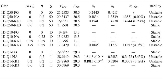
ranges. Table 1 summarises the simulation conditions and the corresponding LSA results, i.e. the stability, growth rate and frequency.
Properties of mixtures for the pulsating detonation simulation and simulation results of
 $\alpha _{i}$
, i.e.
 $\alpha _{i,\textit{sim}}$
. The percentage is the relative difference between
 $\alpha _{i,\textit{sim}}$
and
 $\alpha _i$
. The first column numbers the simulation cases using the spatial dimension of simulation (one dimension), the heat content and the EoS.

Figure 3 presents the postshock pressure history (
 $P_{s}$
), determined as in Hwang et al. (Reference Hwang, Fedkiw, Merriman, Aslam, Karagozian and Osher2000), for the simulations in the large
 $Q$
range. The simulation results were normalised with the steady value
 $P_{s}(t=0)$
. For the PG, the activation energy in the simulation
 $E_{\textit{sim}}$
is 5.24, higher than the critical one
 $E_{\textit{crit}}$
, which should lead to an unstable dynamics according to LSA. In the simulation, the postshock pressure demonstrates strong oscillations around the steady value. Shortly after initiation, the reaction zone decouples from the shock and the postshock pressure decreases to
 $0.54P_{s}(t=0)$
. The detonation reaches a quasi-steady state and is then abruptly re-initiated. As the detonation relaxes from this event, the strength of the detonation oscillates around the steady value. The LSA only predicts one unstable mode for the PG case, with a growth rate of 0.2443 and frequency of 0.4217. As discussed in § 5.1, the LSA would give a number of unstable modes with increasing frequencies. The higher-frequency mode subsequent to the fundamental one has a higher critical activation energy, i.e. 31.0547, which is not triggered in this simulation. However, neither the oscillation amplitude nor frequency was constant in the postshock pressure profile, demonstrating a nonlinear dynamics. When the effect of finite molecular volume was included, the difference between
 $E_{\textit{sim}}$
and
 $E_{\textit{crit}}$
reduces to 1.16 due to the variation of the neutral stability boundary. The simulation shows that the detonation instability is significantly weakened. The amplitude of pressure oscillation increases after initiation and rapidly reaches a constant level. Compared with the PG simulation, the postshock pressure changes from nonlinear to harmonic oscillation. The oscillation frequency is 1.3551, which agrees well with 1.3539 predicted by the LSA. When the effect of inter-molecular attraction force was also included, the postshock pressure still shows harmonic oscillation for
 $A(T_{1})=B$
. Again, the frequency of oscillation agrees well with the LSA prediction with a relative difference of only 0.23 %. In addition, the amplitude of pressure oscillation is slightly lower than that in the NA case, which is
 $0.29P_{s}(t=0)$
in the RK case and
 $0.33P_{s}(t=0)$
in the NA case. The change of pressure amplitude is consistent with the difference in growth rate obtained from LSA, 0.1541 (RK) vs. 0.1834 (NA). As the effect of the inter-molecular attraction force becomes more important for
 $A(T_{1})=3B$
,
 $E_{\textit{crit}}$
surpasses
 $E_{\textit{sim}}$
by 1.25 due to the enhanced stabilising effect of RG. Accordingly, the detonation becomes completely stable as the postshock pressure becomes equal to the steady value. Overall, the neutral stability boundary determined by LSA agrees well with the simulation results, and the stabilising effects of RG were demonstrated in the simulations. When the simulation conditions are close to the stability boundary, the LSA can predict the oscillation frequency, and the growth rate correlates well with the oscillation amplitude.
Postshock pressure of pulsating detonation when
 $Q = 50$
. The steady values
 $P_{s}(t=0)$
of the four cases are respectively 42.06, 42.06, 48.07 and 78.0 for the four models considered. The dashed line represents extrapolation from simulation results.

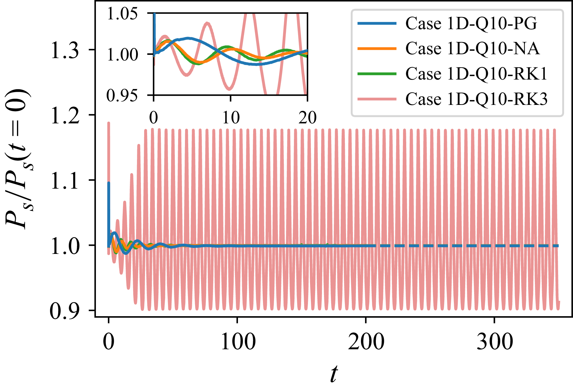
Figure 4 shows the simulation results in the intermediate
 $Q$
range with
 $Q=10$
. According to the LSA,
 $E_{\textit{crit}}$
is lower than
 $E_{\textit{sim}}$
when using PG, NA and RK with
 $A(T_{1})=B$
. The differences are 0.88, 0.69 and 0.46, respectively. In the simulation, the postshock pressures in these cases oscillate after the initiation, but decay quickly as the detonation propagates. Eventually, the postshock pressure approaches the steady value, indicating that stable detonations were established. In the case of RK with
 $A(T_{1})=3B$
,
 $E_{\textit{crit}}$
was 0.46 smaller than
 $E_{\textit{sim}}$
due to the destabilising effect of RG. As predicted by the LSA, the postshock pressure oscillates with increasing amplitude after initiation. Similar to the NA and RK cases with
 $A(T_{1})=B$
in the large Q range, the instability then saturates and undergoes harmonic oscillation. The frequency of the oscillation is 1.1857, which is also close to the prediction of LSA, i.e. 1.1319. The destabilising effects of RG is again validated by simulations.
Postshock pressure of pulsating detonation when
 $Q = 10$
. The steady values
 $P_{s}(t=0)$
of the four cases are respectively 9.97 (PG), 9.97 (NA), 11.39 (RK1) and 18.42 (RK3) for the four models considered. The dashed line represents extrapolation from simulation results.

Postshock pressure of pulsating detonation when
 $Q = 1$
. The steady values
 $P_{s}(t=0)$
are respectively 2.42 (PG), 2.42 (NA), 2.57 (RK1) and 3.29 (RK3) for the four models considered. The dashed line represents extrapolation from simulation results.

Figure 5 presents simulation results for the small
 $Q$
range with
 $Q=1$
. The destabilising effect of the finite molecular volume decreases
 $E_{\textit{crit}}$
from 29.6622 to 28.6149. Since
 $E_{\textit{sim}}$
is 29.3, the detonation is stable for the PG and unstable for the NA model. In the simulation, harmonic oscillation was obtained for the NA model. The frequency is 0.3422, slightly higher than 0.3185, the LSA solution. As the inter-molecular attraction force was included, its stabilising effect increases
 $E_{\textit{crit}}$
to 28.9860 (
 $A(T_{1})=B$
) and 30.6969 (
 $A(T_{1})=3B$
). In the former case, the destabilising effect of the finite molecular volume remains dominant. The detonation is still unstable and exhibits harmonic oscillation. The frequency is 0.3307, close to the LSA prediction of 0.3204. The oscillation amplitude decreases from
 $0.18P_{s}(t=0)$
to
 $0.096P_{s}(t=0)$
, consistent with the growth rate decreasing from 1.8148
 $\times 10^{-2}$
to 8.1815
 $\times 10^{-3}$
in the LSA. In the latter case, the stabilising effect of the inter-molecular attraction force overcomes the destabilising effect of the finite molecular volume, and therefore, the detonation changes from unstable to completely stable. Overall, the pulsating detonation simulation demonstrates the destabilising effect of the finite molecular volume as well as the stabilising effect of the inter-molecular attraction force, as predicted by the LSA.
5.3. Statistical analysis of the reaction zone structure of pulsating detonation
The PDF, ZND solution and linear stability solution of the reaction zone structures, as well as the PDF of detonation speed obtained in case 1D-Q50-PG.

The PDF, ZND solution and linear stability solution of the reaction zone structures, as well as the PDF of detonation speed obtained in cases 1D-Q50-NA (top row) and 1D-Q50-RK1 (bottom row).


In pulsating detonation, the reaction zone structure behind the detonation front is significantly affected by the shock dynamics. To further investigate the variation of the reaction zone structure, figures 6 and 7 present the probability density function (PDF) of pressure, temperature, reaction progress and detonation speed. The three unstable cases with large
 $Q$
were taken as examples. The PDF was calculated with the simulation results after
 $t = 150$
. The steady ZND solution, as well as the real part of the linear stability solution, i.e.
 $z^{*}+\textit{Re}(z^\prime )$
, are also included in these plots as references. In the present theoretical analysis, the steady ZND solution represents the unperturbed result, while the real part of the LSA actually represents the initial perturbation applied to the steady solution. In the PG case presented in figure 6, the detonation speed has two most probable values, one around the CJ speed and the other at approximately 0.88 D
 $_{\textit{CJ}}$
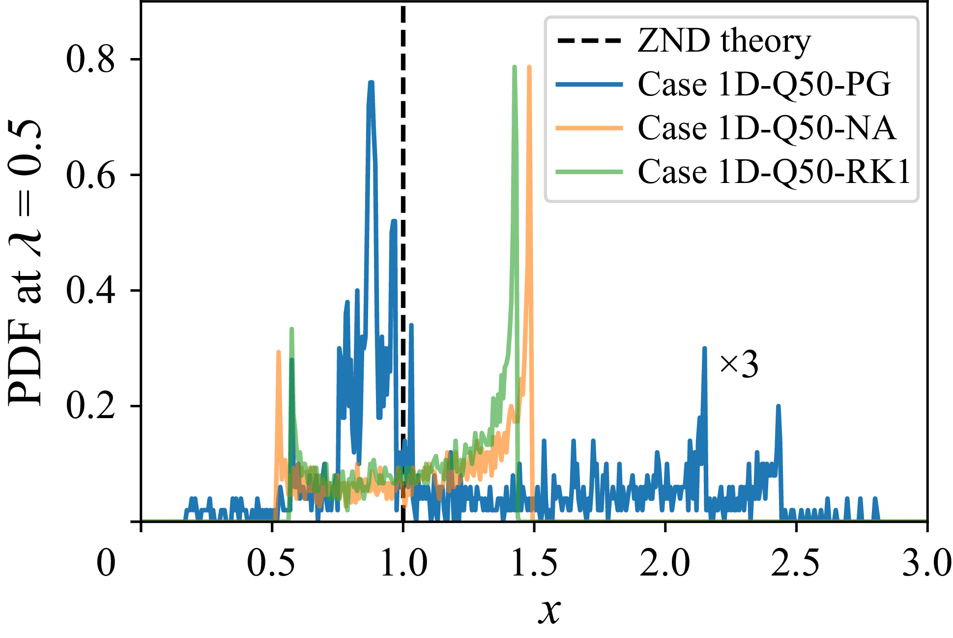
. The detonation can be significantly over-driven despite the low probability density in the high-velocity range. Accordingly, significant variations in the reaction zone structure are observed. During the acceleration stage of the pulsating detonation, larger pressures and temperatures, i.e. more than one fold of increase, and shorter half-reaction length, i.e. up to a five times decrease, are achieved compared with the ZND solution. In contrast, during the deceleration stage, lower pressure and temperature are achieved, and the reaction zone is extended to a wider range. These variations observed in the simulation extend far beyond the profiles of the LSA. Such differences indicate the nonlinear dynamics of this detonation, which cannot be captured with LSA. Despite the significant variations in the reaction zone structure, the PDF plots with the highest probability are close to the ZND solution, indicating that the ZND theory can be a reasonable approximation of the average reaction zone structure for such a nonlinear pulsating detonation. Due to the nonlinear nature of this case, the PDF shows a complex distribution. There are several streaks with relatively high probability density on both the left and right-hand sides of the ZND solution. Figure 8 presents a slice of the PDF of
 $\lambda$
at
 $\lambda = 0.5$
, namely the PDF of the half-reaction length. Two peaks of probability density are found at
 $x\gt 2$
, and one peak is found at around 0.48. These streaks might be related to the multi-frequency oscillation that was observed in the postshock pressure profile, see figure 6.
In figure 7, the PDF for the NA and RK cases are presented. The variations of the reaction zone structure and the detonation speed are less important compared with the PG case. The range of distribution of the reaction zone structures is similar to the initial LSA perturbation. Since the initial perturbation weakens the detonation, its profiles are close to the right edges of the PDF. Such a similarity demonstrates that the pulsating detonation falls in the linear instability regime. The unperturbed profiles, i.e. ZND solutions, are located around the centre of the PDF. Different from figure 6, the probability is quite uniform around the ZND profiles in figure 7, as well as around the CJ speed. This is clearer in the PDF slice plot presented in figure 8. The uniformity is related to the harmonic oscillation of the detonation strength shown in figure 3. The high probability areas are located at the edges of the PDF plot. The two edges correspond to the envelopes of the profiles of
 $P$
,
 $T$
and
 $\lambda$
. The transient profiles are partly located at the two edges, contributing to the higher probability density at these locations.
6. Results for cellular detonation
6.1. Neutral stability boundary of 2-D cellular detonation
In addition to the 1-D LSA, we studied the linear stability in the 2-D scenario, where the transverse instability and cellular structure exist, and the wavenumber
 $k$
is above zero. Figure 9 presents the neutral stability boundary in the activation energy –wavenumber plane for
 $Q=10$
and 50. As
 $k$
increases,
 $E$
first decreases and then increases, indicating the detonation is more sensitive to the transverse than to the longitudinal instability, indicating that a detonation can be stable in the longitudinal direction but unstable within a finite band of wavenumber in the transverse direction. The minimum in each curve thus corresponds to
 $E_{\textit{crit}}$
for 2-D cellular detonation. For PG,
 $E_{\textit{crit}}$
is much smaller for 2-D cellular detonation than for 1-D pulsating detonation, 1.09 vs. 14.18 for
 $Q = 10$
. For
 $Q = 50$
,
 $E$
decreases to below zero as the wavenumber increases, indicating the detonation is always unstable for large wavenumber. Weng & Mével (Reference Weng and Mével2024a
) found that the critical
 $Q$
at which the
 $E$
–
 $k$
curve crosses the
 $x$
-axis is 11.52.
The variation of critical activation energy with wavenumber for (a)
 $Q = 10$
, and (b)
 $Q = 50$
. Here,
 $\gamma ^{0} = 1.2$
. The squares denote the minima of the curves and corresponding values are also provided. For the RK EoS,
 $B$
was fixed at 0.2.

When considering RG,
 $E_{\textit{crit}}$
of 2-D detonation increases, demonstrating the stabilising effects. Specifically, in the intermediate
 $Q$
( = 10) range, both the finite molecular volume and inter-molecular attraction force effects destabilise a pulsating detonation (
 $k=0$
), but tend to stabilise the transverse instability (
 $k\gt 0$
). In the large
 $Q$
( = 50) range, the stabilisation was consistently observed in both longitudinal and transverse directions. In figure 9, it seems that the effect of finite molecular volume has a stronger impact on the
 $E_{\textit{crit}}$
of 2-D detonation. For
 $B=0.01$
, the
 $E_{\textit{crit}}$
–
 $k$
curve is close to the PG-based results. As
 $B$
increases to 0.05,
 $E_{\textit{crit}}$
stops dropping to a negative value for
 $Q=50$
. By further doubling
 $B$
(from 0.05 to 0.1, 0.2),
 $E_{\textit{crit}}$
increases by tens of per cent (
 $Q=10$
) or several folds (
 $Q=50$
). In contrast, fixing
 $B = 0.2$
and increasing
 $A(T_{1})$
from 0.2 to 0.6 leads to a relatively small change of
 $E_{\textit{crit}}$
. Nevertheless, the combined impact of the two RG effects still has a more significant stabilising effect than the finite molecular volume alone. When
 $A(T_{1})=0.6$
and
 $B=0.2$
,
 $E_{\textit{crit}}$
of 2-D detonation was found to be even larger than the critical value of a PG detonation in the longitudinal direction, 25.61 vs. 25.26. Therefore, a cellular detonation in RG can be more stable than a pulsating detonation in PG. In other words, the PG-based analysis might largely over-predict the instability of cellular detonation under certain conditions.
By computing the minima of
 $E$
with respect to
 $k$
, the complete neutral stability boundary for 2-D cellular detonation in RG was obtained, see figure 10. The 1-D and 2-D stability boundaries of PG are also presented for reference. In the
 $E$
–
 $Q$
plane, the transverse instability changes the neutral stability boundary from C-shape in the 1-D case to hyperbola-like in the 2-D case, significantly reducing the parameter space for stable detonation. There is a maximum
 $Q = 11.52$
in the 2-D boundary which corresponds to a maximum Mach number in the
 $M$
–
 $\theta$
plane (Weng & Mével Reference Weng and Mével2024a
), denoted
 $M_{\textit{2D,max}} (= 3.22)$
in this work. With the RG effects, the neutral stability boundary for 2-D cellular detonation recovers a C-shape in the
 $E$
–
 $Q$
plane, and covers a much wider range of Mach number in the
 $M$
–
 $\theta$
plane. In the small
 $Q$
range, the 2-D stability boundary of RG is close to the PG one. As
 $Q$
increases, the stabilising effect of RG becomes more significant. As observed in figure 9, the finite molecular volume has a dominant impact on the variation of the stability boundary. Nonetheless, when the inter-molecular attraction force is included, it shifts the neutral stability boundary to the stable side, and thus further stabilises the detonation in the whole parameter space considered herein. In the
 $M$
–
 $\theta$
plane, the critical reduced activation energy of RG does not decrease monotonically with
 $M$
as for the PG. Instead, it firstly decreases and then increases with the Mach number; see results of 1-D stability boundary in figure 1.
Neutral stability boundary in
 $E$
–
 $Q$
and
 $M$
–
 $\theta$
planes for 2-D detonation obtained with RG models. The PG results by Short & Stewart (Reference Short and Stewart1998) and Weng & Mével (Reference Weng and Mével2024a
) are also shown. Here,
 $B$
was fixed as 0.2 for the RK model and
 $\gamma ^{0} = 1.2$
.

The neutral stability boundary in LSA has been related to the cellular dynamics. Weng & Mével (Reference Weng and Mével2024a
) identified four regimes using the 1-D and 2-D stability boundaries in the
 $M$
–
 $\theta$
plane for PG, as show in figure 11. The definitions and characteristics of these regions are:
-
(i) stable region: on the left of the 2-D stability boundary. Detonation is steady and planar;
-
(ii) linearly instability region: between the 1-D and 2-D stability boundaries, with Mach number smaller than
$M_{\textit{2D,max}}$
. The detonation is characterised by a regular cellular structure. The cell size can be well predicted with the most unstable wavelength in LSA; -
(iii) weakly nonlinearly instability region: between the 1-D and 2-D stability boundary, with Mach number larger than
$M_{\textit{2D,max}}$
. The detonation has a regular cellular structure, but the cell size increases during propagation. The LSA prediction is limited to the initial cell size; -
(iv) nonlinearly instability region: beyond the 1-D stability boundary. There is a rapid transition from steady planar detonation to cellular detonation due to (i) interaction between longitudinal and transverse instabilities; (ii) large perturbation introduced by local explosions; (iii) appearance and dominance of high-frequency modes of transverse instability.


The 1-D and 2-D neutral stability boundaries for PG and RG. The stability map was defined for PG; NA:
 $B = 0.2$
. RK:
 $A(T_{1}) = 3B$
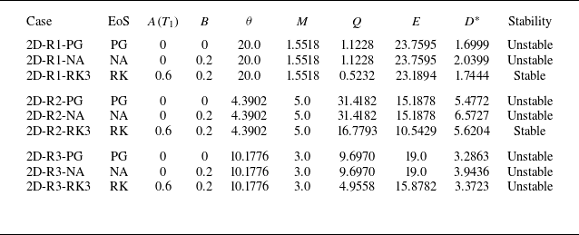
. Symbols denote the simulation conditions in the following section and their coordinates are given in table 2. Here,
 $\gamma ^{0} = 1.2$
.

To better characterise the impact of the RG effects on the cellular structure, both the 1-D and 2-D stability boundaries are plotted in the stability map, see figure 11. Considering only the finite molecular volume, the stability boundaries at large
 $\theta$
are close to the PG ones. Due to the disappearance of
 $M_{\textit{2D,max}}$
in the 2-D stability boundary, the stable region (0) extends to much higher Mach number, and regimes (1) and (2) cannot be clearly separated. The 1-D boundary of NA enters region (3) of PG at large
 $M$
, decreasing the area of region (3) for NA. A nonlinearly unstable detonation for PG can thus be weakly nonlinear in the NA case. Further including the effect of the inter-molecular attraction force, the 1-D and 2-D boundaries of the RK EoS are even more significantly shifted towards the PG region (3). At large
 $\theta$
, the linear instability region (1) of RK falls in the nonlinear PG instability region (3). Similarly, at large
 $M$
, the weakly nonlinear instability region (2) of RK also overlaps with the PG nonlinear instability region (3). As in the NA case, regions (1) and (2) are difficult to differentiate. The dynamics of the RG detonation in these two regions is further studied in the next section via numerical simulation. One more feature is that the 1-D and 2-D boundaries of RK become much closer than in the PG and NA cases. This means the prediction of LSA for cell size would be limited to a narrower parameter space. Regardless of the variation of the stability regions due to RG effects, the nonlinear unstable region remains dominant in the
 $M$
–
 $\theta$
plane.
Properties of mixtures for the cellular detonation simulations;
 $\gamma ^{0} = 1.2$
. The first column numbers the simulation cases using the spatial dimension of simulation (two dimensions), the regime in the PG stability map (R1-R3) and the EoS.

6.2. Detonation flow fields in numerical simulation
Numerical simulations for 2-D cellular detonation were performed using both the PG and RG models. The simulation conditions were selected based on the results of LSA, as shown in figure 11 and summarised in table 2. These cases are numbered using the spatial dimension of simulation (i.e. 2-D), the regime in the PG stability map of figure 11, i.e. R1–R3 and the EoS. The first group falls in the linearly stable region (1) for PG. We fixed the Mach number at 1.5518 and the reduced activation energy as 20.0, and repeated the simulation with the PG, NA and RK models. Due to the variation of neutral stability boundaries, the detonation was expected to be unstable for the NA EoS but stable for the RK EoS according to LSA. Similarly, the second group was placed in the weakly nonlinearly instability region (2) of PG. The detonation was expected to be unstable for the PG and NA EoSs but stable for the RK EoS. The third group is located in the nonlinearly instability region (3). Therefore, the detonation should be unstable for all models. When
 $M$
and
 $\theta$
are fixed, it is noted that the heat content and activation energy are smaller for the RK model and the same for the NA and PG models, because the effect of the inter-molecular volume leads to a much higher detonation speed and frozen sound speed.
The temperature, pressure and schlieren fields of cases 2D-R1-PG, 2D-R1-NA and 2D-R1-RK3 at
 $t = 440$
.

Figure 12 presents the transient temperature, pressure and schlieren fields for cases 2D-R1-PG, 2D-R1-NA and 2D-R1-RK3. The simulation time is 440, but the locations of the detonation front are different due to the different detonation speeds. When using the PG and NA models, the detonation front is quite close to a planar one, but typical triple-wave structures still exist. The incident shock, Mach stem and transverse shock, which are marked in figure 12, are connected via the triple point. Due to the difference in shock strength of different shock waves, the reaction zone field demonstrates a typical keystones structure, as shown in the temperature field. In the NA case, the triple points are distributed more uniformly on the detonation front than in the PG case, indicating a more regular cellular structure. However, in the RK case, a completely planar detonation without a triple-wave structure was obtained after a long simulation time. This is consistent with the prediction of the LSA, which indicates that this simulated case falls in the stable regime. The perturbation from numerical error did not grow, and the distortion of the detonation front during its propagation did not occur.
The temperature, pressure and schlieren fields of cases 2D-R2-PG, 2D-R2-NA and 2D-R2-RK3 at
 $t = 160$
.

The temperature, pressure and schlieren fields of cases 2D-R3-PG, 2D-R3-NA and 2D-R3-RK3 at
 $t = 240$
.

The simulation results for cases 2D-R2-PG, 2D-R2-NA and 2D-R2-RK3 at
 $t = 160$
are presented in figure 13. Compared with cases in regime (1), the detonation becomes more unstable when using the PG model. There is a larger difference in the strength of the incident shock and the Mach stem. A double-Mach reflection structure is observed. Along the slip line, vortex pairs are formed behind the Mach stem. While a one-step chemistry was used, these structures are qualitatively consistent with experimental results for weakly unstable detonation, like in hydrogen–oxygen–argon mixtures (see figures 2 and 3 in Pintgen et al. (Reference Pintgen, Eckett, Austin and Shepherd2003), chapter 4 in Austin (Reference Austin2003)). The vortex pair induces a forward jet toward the Mach stem, which may interact with the leading shock front. Such an interaction can lead to shock wave bifurcation, which is one of the mechanisms for the birth of a new triple point, and generally leads to more irregular cellular structures (Mach & Radulescu Reference Mach and Radulescu2011; Lau-Chapdelaine, Xiao & Radulescu Reference Lau-Chapdelaine, Xiao and Radulescu2021; Sow, Lau-Chapdelaine & Radulescu Reference Sow, Lau-Chapdelaine and Radulescu2021). Considering the finite molecular volume, the detonation was significantly stabilised. The detonation front is less distorted compared with the PG case. Mach reflection structures are formed with weak transverse shocks, which are not as visible in the schlieren field. Around the slip line, no obvious vortex can be observed. In the temperature or schlieren fields, the vortical flow behind the PG detonation is replaced by a number of cellular patterns in the NA case. Overall, the structure of the detonation front is closer to those obtained in cases 2D-R1-PG and 2D-R1-NA. In previous studies, the formation of vortex pair and forward jet have been related to the Mach number, isentropic coefficient and the Reynolds number (Lau-Chapdelaine et al. Reference Lau-Chapdelaine, Xiao and Radulescu2021). In this work, the Mach number of the steady detonation is fixed for a series of cases. The Reynolds number can be defined with the numerical viscosity, which is a function of the numerical scheme and mesh size. The Reynolds number is expected to be at the limit of large value due to the small numerical viscosity compared with the physical viscosity (Lau-Chapdelaine et al. Reference Lau-Chapdelaine, Xiao and Radulescu2021). Therefore, the isentropic coefficient becomes a major factor governing the appearance of the vortex pair and the forward jet. The isentropic coefficient is constant at 1.2 in the PG simulations, whereas it is equal to 1.44 (NA) and 1.73 (RK) at the initial state, and to 3.09 (NA) and 4.57 (RK) at the von Neumann state. The significantly higher isentropic coefficient in RG helps in explaining the difference in the simulation results. In the RK case, a completely planar detonation was again obtained, which agrees with the LSA prediction.
Simulation results at
 $t=240$
for cases 2D-R3-PG, 2D-R3-NA and 2D-R3-RK3 are shown in figure 14. For PG, the detonation becomes more unstable than in cases 2D-R1-PG and 2D-R2-PG. The detonation front is distorted and very irregular due to more frequent bifurcations. As seen in the temperature field, the reaction zone exhibits a saw-tooth-like structure. In addition, the shocked mixture cannot be consumed within a short period upon shock compression, resulting in unreacted pockets. These structures show similarity with the OH fluorescence images for highly unstable detonation, such as in hydrogen–oxygen(–nitrogen) mixtures at an initial pressure of 20 kPa, see figure 4 of Pintgen et al. (Reference Pintgen, Eckett, Austin and Shepherd2003) and chapter 5 or figure 5.11 of Austin (Reference Austin2003). Considering the finite molecular volume, the detonation front remains quite irregular but is less unstable than in the PG case. There are fewer bifurcations in the detonation front. For the RK gas, the stabilising effect of RG is much stronger, and the simulation results are similar to those in case 2D-R2-NA. The detonation front is highly regular, with the triple points distributed uniformly along the detonation front.
6.3. Numerical cellular structure characterisation
The stability of the cellular detonation was also characterised through numerical soot foils, which were recorded using the maximum pressure history. The complete soot foils for all cases from table 2 are presented in Appendix. The soot foil region between 850 and 1050 is magnified in figure 15 for cases 2D-R1-PG and 2D-R1-NA. Since the instability develops spontaneously without prescribed perturbation, the cellular structure becomes visible around
 $x = 200$
in both PG and NA cases. At an early stage, the cell size is not uniform, but as the detonation propagates, the trajectories of weak triple points disappear gradually, indicating smaller cells merging with larger cells. After
 $x=800$
, the cellular structure becomes highly regular without an obvious change in the cell size. To perform a statistical analysis, the cell size (
 $S_{\textit{cell}}$
) was measured between
 $x=950$
and
 $x=1050$
. The distribution of the cell size in this range is presented in figure 15. In the PG case, the cell size ranges from 9.65 to 11.50, and the average cell size is 10.73
 $\pm$
0.44. In the NA case, a narrower distribution of the cell size was obtained compared with the results for the PG case, which indicates a more regular cellular pattern and demonstrates the stabilising effect of the finite molecular volume. Specifically, the cell size is between 11.10 and 12.02, while the average value is 11.54
 $\pm$
0.20.
Numerical soot foils and PDF of cell size of cases 2D-R1-PG (a) and 2D-R1-NA (b). The cell size was measured for
 $x\in (950, 1050)$
. The dashed lines denote the average values, which are 10.73 (PG) and 11.54 (NA). The orange curve and circle denote the growth rate and predicted cell size obtained in LSA, respectively.

In our previous work (Weng & Mével Reference Weng and Mével2024a
), it has been shown the cell size can be reasonably predicted with LSA when the mixture falls in the first regime of figure 10. The prediction is achieved by searching the wavelength with the maximum growth rate, i.e.
 $S_{\textit{cell}} = 2\pi /k$
, and at the same time allowing an integer number of half-cell to be present in the channel. The growth rate and cell size prediction through LSA are also plotted in figure 15. In both cases, there is only one unstable mode. The growth rate first increases, then decreases as the cell size increases. The LSA under-predicts the cell size in both cases. For PG, the prediction is 10.0, which is approximately 9.9 % lower than the average cell size. In the NA case, the prediction is 10.71 and is approximately 7.1 % lower than the average cell size. The cell size in the numerical simulation tends to be distributed in the right branch of the growth rate curve. This observation is consistent with Barkhordari & Farshchi’s (Reference Barkhordari and Farshchi2013) work. They claimed that the cell size should be determined based on the rate of change of the
 $\alpha _{r}$
–
 $S_{\textit{cell}}$
curve instead of the amplitude of the growth rate. However, no specific method using such a rate of change is available in the literature. Despite the error in cell size prediction, the LSA effectively captures the impact of RG effects on the cell size variation. In the simulations, the average cell size for the NA case was 7.5 % larger than that of the PG case, while the LSA predicted an increase of 7.1 %. These findings indicate that our extension of the LSA from PG to RG successfully retains the essential physics of the RG effects. The discrepancy of the theoretical prediction primarily stems from differences between the assumption in the LSA and the nonlinear nature of the actual reactive Euler equations.
Numerical soot foils and PDF of cell size of cases 2D-R2-PG (a) and 2D-R2-NA (b). The cell size was measured for
 $x\in (950, 1050)$
. The dashed lines denote the average values which are 17.95 (PG) and 9.57 (NA). The orange curve and circle denote the growth rate and predicted cell size obtained in LSA, respectively.

Figure 16 shows the numerical soot foils for cases 2D-R2-PG and 2D-R2-NA. In the PG case, the cellular structure can be observed around
 $x=100$
. The cell size is quite small at the birth of the cellular structure. As the detonation propagates, the cell size grows and stabilises at a larger value. The cell size was also measured in the range of 950–1050. The average cell size is 17.95
 $\pm$
3.51, which is 163 % larger than the prediction with LSA, i.e. 6.82. The cell shows irregular distribution with a maximum size of 23.58 and a minimum size of 8.48. According to Weng & Mével’s (Reference Weng and Mével2024a
) findings, the LSA predicts better the cell size formed at the early stage around
 $x=100$
. During the detonation propagation, the nonlinear dynamics of the detonation gets progressively activated and leads to larger cellular structures. In the NA case, the appearance of the cellular structure is significantly delayed due to the stabilising effect of RG. Moreover, no obvious growth of the cell size is observed in the simulation. The cellular structure is very regular, with cell size ranging from 8.19 to 11.48. The average cell size is 9.57
 $\pm$
0.51, which agrees well with the prediction of LSA, i.e. 9.09. These characteristics are actually more similar to those in regime (1), such as cases 2D-R1-PG and 2D-R1-NA. Recalling the definition of regimes (1) and (2) in the stability map (figure 11), they were separated by
 $M_{\textit{2D,max}}$
in the PG case. Since
 $M_{\textit{2D,max}}$
disappears in the LSA of the NA case, it should be expected that regime (2) would be partly or completely replaced by regime (1). The variation of the stability map thus explains the change of cellular dynamics in the NA case as compared with the PG case. It also indicates that the use of
 $M_{\textit{2D,max}}$
to separate regimes (1) and (2) is a rational choice for both PG and NA.
Numerical soot foils and PDF of cell size of cases 2D-R3-PG (a), 2D-R3-NA (b) and 2D-R3-RK3 (c). The cell size was measured for
 $x\in (950, 1050)$
. The dashed lines denote the average values, i.e. 12.84 (PG), 10.28 (NA) and 12.49 (RK). The orange solid and dashed curves denote the growth rate of the fundamental mode and the higher-frequency mode, respectively. The orange circle is the predicted cell size.

Figure 17 presents the numerical soot foils for cases 2D-R3-PG, 2D-R3-NA and 2D-R3-RK3. The PG case has been presented in Weng & Mével (Reference Weng and Mével2024a
), but the simulation was repeated here with higher resolution, i.e. from 1/32 to 1/48. In the PG and NA cases, a much finer cellular structure was formed at the initial stage, see the supplementary materials. The size of these fine cells is comparable to the half-reaction length of the ZND model. As the detonation propagates, the cellular structure grows rapidly. However, compared with the cellular structure of case 2D-R2-PG, a highly irregular cellular structure was obtained. The diamond shape of the cellular structure was hardly seen in these two cases. Instead, due to the frequent bifurcations in the detonation front as shown in figure 14, triple point trajectories penetrate into a diamond-like cell, cutting it into several cells with large aspect ratios. This process is further illustrated in figure 18 using case 2D-R3-PG as an example. The trajectories resulting from the bifurcations of the detonation front were denoted with a blue arrow. The start of the bifurcation seems quite random, with some of them located inside a cell and others located at the edge of the cell. When one cell cycle terminates, these trajectories either disappear or penetrate into the next cell cycle, as denoted with the black arrow. The irregularity was also reflected in the distribution of the cell size. In the PG case, the cell size ranges from 3.51 to 24.64 with the nominal value of 12.84
 $\pm$
4.70, while in the NA case, the cell size varies from 2.63 to 20.84 with the nominal value of 10.28
 $\pm$
3.99. In LSA, a notable feature is that a higher-frequency unstable mode appears in the PG and NA EoS cases, which is plotted as dashed lines in figure 17. For PG, the growth rate of the higher-frequency mode is even higher than the fundamental mode, which results in a much smaller cell structure in the prediction, i.e. 2.91. Again, this prediction is closer to the size when the cellular structure is initially formed. In the NA case, the higher-frequency mode still exists and corresponds to a smaller cell size. However, due to the stabilising effect of RG, the growth rate of the fundamental mode remains dominant. In this case, the LSA actually gives a good approximation of the average cell size, i.e. 10.0. In the RK case, including the inter-molecular attraction force further stabilises the detonation. A regular cellular structure was obtained in the simulation. The higher-frequency mode changes from unstable to stable. Quantitatively, the cell size is limited to a narrow range, i.e. from 11.96 to 12.96. The average cell size is 12.49
 $\pm$
0.18, which agrees well with the LSA prediction of 11.11.
The variation of the detonation front in case 2D-R3-PG. The arrows denote the occurrence of front bifurcation and its penetration into the following cells.

7. Discussion
7.1. On the coupling of the shock dynamics and chemical reaction
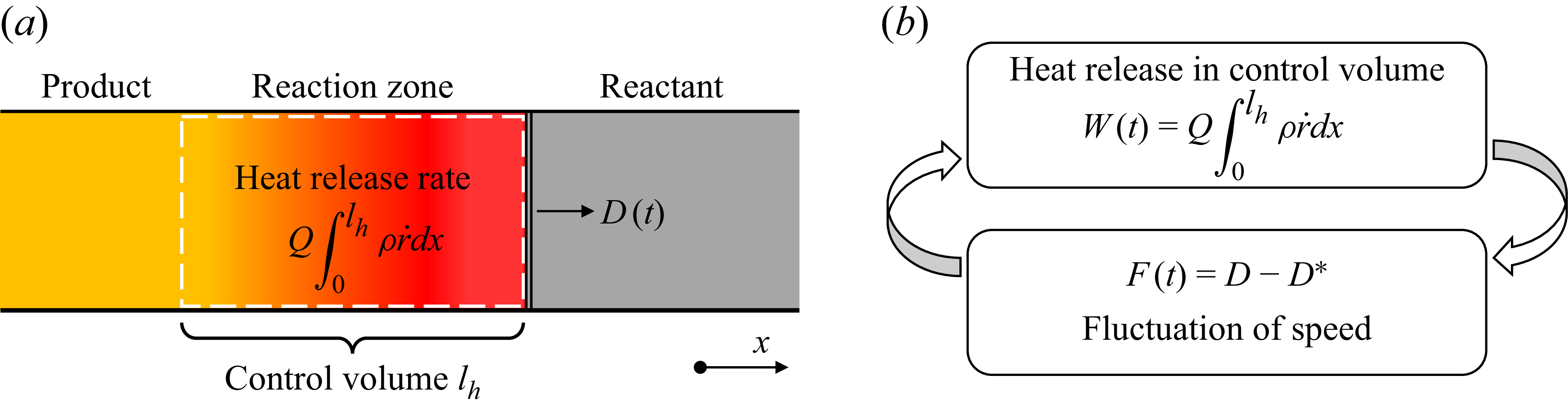
Illustration of (a) the control volume for the oscillator model, as well as (b) the interaction between heat release and detonation propagation.

Considering that detonation propagation is essentially governed by shock compression and auto-ignition, the detonation instability originates from the interaction between the heat release and shock dynamics. These two aspects and their interactions should be further investigated to explain the RG effects on detonation stability. To measure these interactions, we utilise the concept of the oscillator model in mechanics. The idea was first proposed by Zhang et al. (Reference Zhang, Chue, Lee and Klein1998) for 1-D pulsating detonation and is illustrated in figure 19. The heat release from a control volume behind the shock wave is considered as the driver for the change of the detonation dynamics. By deriving the integral form of the conservation equation for the control volume, they obtained a second-order differential equation for the fluctuation of detonation speed analogous to the governing equation for the nonlinear oscillator in mechanics. The driving force for the oscillator is the heat release (
 $W(t)$
), while the displacement of the oscillator corresponds to the fluctuation of the detonation speed (
 $F(t)$
). The definitions are
 $$\begin{align}W(t) &= Q\int _{0}^{l_{h}} \rho (t)\dot {r}(t) \text{d}x,\end{align}$$
 $$\begin{align}F(t) &= D(t) - D^*,\end{align}$$
where
 $l_{h}$
is the width of the control volume, which should be large enough to cover the whole reaction zone. In this work, it was fixed as 20. The resonant coupling of the heat release and shock dynamics can thus be described with
 \begin{equation} J=\frac {1}{\tau D_{\textit{CJ}}} \int _0^\tau W \dot {F} \text{d}t, \end{equation}
where
 $\tau$
is the time range for the integration, typically several folds of the oscillation period. A positive
 $J$
refers to an unstable detonation, and the increase of
 $J$
was related to the variation of instability patterns from a harmonic to an irregular chaotic dynamics (Zhang et al. Reference Zhang, Chue, Lee and Klein1998).
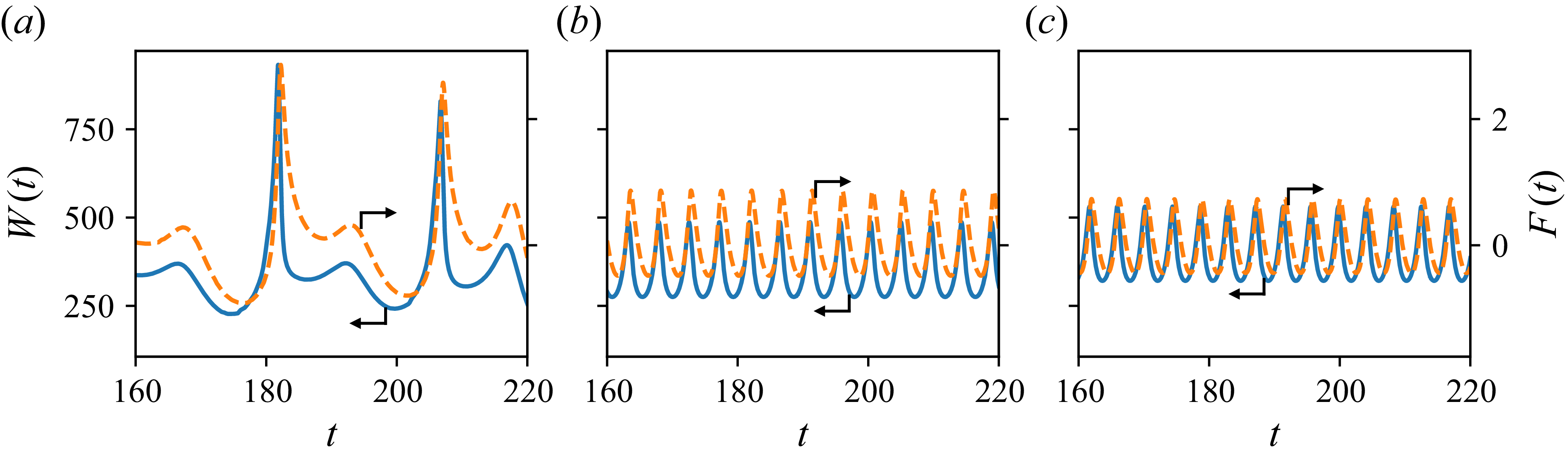
The heat release and fluctuations of detonation speed in cases 1D-Q50-PG, 1D-Q50-NA and 1D-Q50-RK1. The values of the
 $J$
parameter were respectively 9.542, 2.617 and 2.073 for the three cases. (a) Case 1D-Q50-PG, (b) Case 1D-Q50-NA and (c) Case 1D-Q50-RK1.

Figure 20 presents the fluctuation of heat release and detonation speed in the large
 $Q$
range for the cases 1D-Q50-PG, 1D-Q50-NA and 1D-Q50-RK1. Consistent with the postshock pressure profiles, the results for PG are characterised by large-amplitude and low-frequency fluctuations, while the results of the NA and RK cases show high-frequency, harmonic oscillations. In all cases, a phase difference, defined as the time difference between the peaks of
 $W$
and
 $F$
over the oscillation period, was observed between heat release and the detonation speed. The heat release, being the driving force, has a leading phase over the displacement, i.e. the detonation speed. During acceleration, the phase lag is small, indicating a prompt response of the detonation speed to the increase of heat release rate. During deceleration, the heat release rate drops very quickly, which has a damping effect on the detonation propagation. The response of the detonation front to this damping is relatively slow. Compared with the PG simulation, the RG effects tend to decrease the amplitude of the detonation speed oscillation. The average heat release rate for NA is similar to that of the PG (345.5 vs. 340.5), whereas the RK model gives a much higher average heat release rate (390.1). In addition to the value of
 $W$
and
 $F$
, the phase difference between them is also increased for the RG, indicating a weaker heat release–shock dynamics coupling. For PG, heat release and velocity variations are almost in phase, with only 1.61 % phase difference relative to the oscillation period. However, in the NA and RK cases, the phase differences respectively increase to 7.06 % and 7.62 % of their respective periods. To consider the overall impacts, the
 $J$
parameter was calculated as 9.542, 2.617 and 2.073, respectively, for PG, NA and RK. The decrease of
 $J$
indicates the weakening of the pulsating detonation instability as observed by Zhang et al. (Reference Zhang, Chue, Lee and Klein1998), further demonstrating the stabilising RG effects in the large
 $Q$
range.
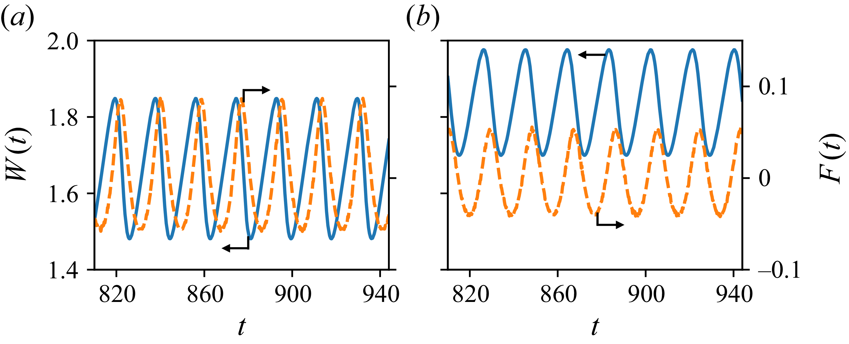
A similar analysis was performed for two unstable cases, 1D-Q1-NA and 1D-Q1-RK1, in the small
 $Q$
range with
 $Q=1$
. The
 $W(t)$
and
 $F(t)$
results are presented in figure 21. The detonation is stable when considering for PG, resulting in constant
 $W=1.66$
and
 $F=0$
. At small
 $Q$
, both
 $W$
and
 $F$
are more than one order of magnitude smaller than for large
 $Q$
. The average heat release rate for NA is similar to that for PG, i.e. 1.66, and is higher in the RK case, i.e. 1.83. From 1D-Q1-PG to 1D-Q1-NA, the finite molecular volume is destabilising, consistent with the results in § 5.2, which results in a positive amplitude of the velocity oscillation. From 1D-Q1-NA to 1D-Q1-RK1, the inter-molecular attraction forces have a stabilising effect. Accordingly, the amplitude of the speed oscillation decreases, and the phase lag between
 $W$
and
 $F$
increases from 15.84 % to 18.21 % relative to the oscillation period. The
 $J$
parameters are 0 in 1D-Q1-PG,
 $1.23\times 10^{-3}$
in 1D-Q1-NA and
 $5.69\times 10^{-4}$
in 1D-Q50-RK1. The stabilising/destabilising RG effects are again well captured by the
 $J$
parameter.
The heat release rate and fluctuations of detonation speed in cases 1D-Q1-NA and 1D-Q1-RK1. The values of the
 $J$
parameter were respectively
 $1.23\times 10^{-3}$
and
 $5.69\times 10^{-4}$
for the two cases. (a) Case 1D-Q1-NA, (b) Case 1D-Q1-RK1.

While the oscillator model was originally developed for 1-D pulsating detonation, it was also applied to the 2-D cellular detonation using the data in the centreline of a cell cycle. It should be noted that the centreline might be tilted or curved relative to the
 $x$
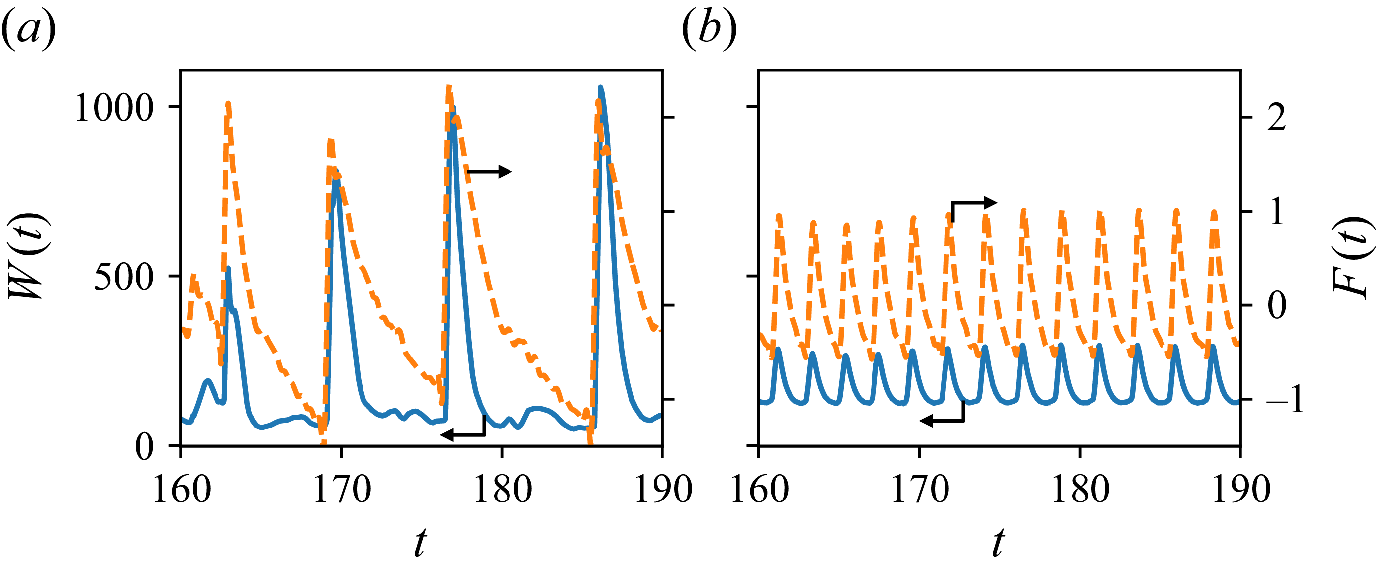
axis, especially for irregular cellular structures. For simplicity, the data at the top and bottom walls were used, which well represent the detonation dynamics at the centreline of a cell cycle. The following discussions are based on the data at the top wall, while a similar analysis for data at the bottom wall is provided in the supplementary materials. Figure 22 presents the variation of
 $W$
and
 $F$
in cases 2D-R2-PG and 2D-R2-NA. Again, since the detonation in case 2D-R2-RK3 is stable, constant
 $W=128.8$
and
 $F=0$
were obtained. The average heat release of the PG and NA cases was again close, i.e. 172.2 vs. 170.3, which was higher than that for the RK simulation. Section 6.2 has shown that the effect of finite molecular volume results in a more stable detonation compared with the PG simulation. Such a stabilising effect was again correlated with the decreasing amplitude of detonation speed oscillation and the increase of phase difference between
 $W$
and
 $F$
. In the NA case, the heat release rate has a leading phase of 2.14 % relative to the oscillation period over the detonation speed. However, in the PG case, the heat release rate has the same or deferred phase compared with the speed oscillation. The average phase difference is –2.23 % relative to the oscillation period. The reason is that the detonation propagation is not only driven by the heat release as in 1-D pulsating detonation, but also affected by the successive convergence and divergence of the 2-D detonation front. At the beginning of the cell cycle, the reflection of the detonation front or triple point at the bottom wall was not included in the oscillator model, which can contribute to the acceleration of the detonation front in addition to the heat release.
The heat release rate and fluctuations of detonation speed measured at the top wall in cases 2D-R2-PG and 2D-R2-NA. The values of the
 $J$
parameter were respectively 23.75 and 3.44. (a) Case 2D-R2-PG, (b) Case 2D-R2-NA.

Figure 23 shows the variation of
 $W$
and
 $F$
at the top wall in cases 2D-R3-PG, 2D-R3-NA and 2D-R3-RK3. The highly irregular cellular structures in case 2D-R3-PG, as shown in figure 16, result in complex variations of the heat release rate and detonation speed. Notably, the heat release rate covers several orders of magnitude, and the periods of the cell cycle also demonstrate large variations. The average heat release rate is 47.9 in case 2D-R3-PG, and decreases to 38.9 in case 2D-R3-NA and 24.3 in case 2D-R3-RK3. Since the finite molecular volume and inter-molecular attraction forces stabilise the detonation, the amplitude of speed oscillation becomes smaller in NA and RK cases. In addition, the phase difference between
 $W$
and
 $F$
increases from 2.90 % (PG) to 4.58 % (NA) and 13.06 % (RK). Accordingly, a decreasing trend of the
 $J$
parameter is also observed for these three cases, which is consistent with the stabilising effect of RG. Quantitatively, the
 $J$
parameter is 14.18 in the PG case and decreases to 2.69 and 1.53 in the NA and RK cases, respectively.
The heat release rate and fluctuations of detonation speed measured at the top wall in cases 2D-R3-PG, 2D-R3-NA and 2D-R3-RK3. The values of the
 $J$
parameter were respectively 14.18, 2.69 and 1.53. (a) Case 2D-R3-PG, (b) Case 2D-R3-NA and (c) Case 2D-R3-RK3.

Generally, the above results demonstrate that the oscillator model can effectively quantify the heat release and the shock dynamics, as well as their interactions for both 1-D pulsating detonation and 2-D cellular detonation. The stabilising effect of RG on detonation propagation is correlated with the decreasing amplitude of speed oscillation, increasing the phase difference between
 $W$
and
 $F$
, and decreasing the trend of the
 $J$
parameter. The average heat release rate is overall close between the PG and NA cases, while the inter-molecular attraction forces might lead to a higher or lower average heat release rate depending on the mixture properties. Nevertheless, the quantitative difference in heat release rate appears to be a secondary effect compared with the speed oscillation amplitude and phase difference. Last but not least, it should be noted that the oscillator model has been strictly derived from fundamental conservation equations for 1-D pulsating detonation, but not for 2-D cellular detonation. Due to the co-existence of a Mach stem and incident shock in the cellular detonation front, the acceleration of the Mach stem and deceleration of the incident shock take place simultaneously. As a result, the driving and damping effects on the oscillator would be cancelled out in the integral form of the governing equations, and the interaction between the heat release and shock dynamics cannot be well observed in the oscillator model. The improvement of the oscillator model for multi-dimensional cellular detonation is left to future work.
7.2. The effect of initial perturbation on the formation cellular structure
In figures 12 and 13, planar detonations were obtained in the 2-D simulation using the RK model. While the simulation results agree well with the prediction of LSA, it is worth studying whether the planar detonation can still be established as nonlinear instability is triggered when subjected to large-amplitude perturbations. As mentioned in § 4, the simulation results presented in § 6 are initiated using the steady solution without a prescribed perturbation. The instability develops spontaneously during propagation due to the truncation errors of the numerical schemes. In this section, the planar detonation of the RK model is repeated but with a different initiation set-up. A sine wave perturbation is applied at the detonation front. The perturbed shock position is described as
 $x_{s,0} + A_{\textit{pert}}*\sin (2\pi y/10)$
, in which
 $x_{s,0}$
refers to the unperturbed shock location and is equal to 50. The postshock state is again the ZND solution but shifted horizontally based on the position of the detonation front. The wavelength of the perturbation was fixed at 10, which corresponds to an unstable mode in the LSA for both the IG and NA cases, as shown in figures 15 and 16. The amplitudes of the perturbation, i.e.
 $A_{\textit{pert}}$
, were taken as 1, and 10. It should be noted that the first amplitude is comparable to the half-reaction length, while the second amplitude is much larger than the half-reaction length. From the perspective of direct detonation initiation, the area of the driver section is the same regardless of the perturbation amplitude, and therefore, the evolution of the perturbed detonation is related to the stability characteristics of the mixture instead of the initiation energy. To reduce the amount of computation resources, the domain width was reduced to 20, which fits two periods of the sine wave perturbation.
Figure 24 presents the evolution of the temperature fields after applying a sine wave perturbation for case 2D-R1-RK3 with
 $A_{\textit{pert}}=1, 10$
. For
 $A_{\textit{pert}}=1$
, high-temperature spots develop behind the trough areas of the perturbed detonation at
 $t=2$
. The interaction of shock waves at the detonation front was observed at latter times. However, the triple-wave structure and the triple point of cellular detonation cannot be maintained, and eventually the detonation front becomes planar after
 $t=10$
. For
 $A_{\textit{pert}}$
much larger than the half-reaction length, strong blast waves are formed at the crest regions of the detonation front, and decoupling from the reaction zone is observed. The interaction of the blast waves with each other leads to high-temperature spots in the trough areas, from which the reaction front accelerates and re-coupled with the blast wave. The re-coupling of reaction zone and shock wave leads to a marginal detonation at
 $t=25$
, which eventually decays to a planar detonation after
 $t=60$
. It is clear that the perturbation with larger amplitudes takes longer time to decay, but all perturbations stabilise after propagating for approximately 100 times of the half-reaction length.
Figure 25 presents a similar analysis for case 2D-R2-RK3. The evolutions of the temperature field are overall similar to those in case 2D-R1-RK3. When the perturbation amplitude is similar to the reaction length scale, high-temperature spots develop behind the trough areas behind the detonation front. Triple-shock-like structures can be observed but they decay as the detonation propagates. A completely planar detonation is obtained after
 $t=20$
. When applying a larger amplitude of perturbation, strong blast waves are first formed at the crest region of the shock front, behind which instability develops at the reaction front, resulting in small-scale vortices. Then, the reaction zone acceleration is observed in the trough area of the shock front. Either cellular detonation or marginal detonation was created temporarily, due to the re-coupling of the shock wave and reaction zone. These structures are subsequently damped, which leads to planar detonation again. Planar detonation is also achieved after propagating for approximately 100 times the half-reaction length.
The temperature field when the detonation of case 2D-R1-RK3 was subjected to sine wave perturbations;
 $A_{\textit{pert}}=1$
(a) and 10 (b).

The temperature field when the detonation of case 2D-R2-RK3 was subjected to sine wave perturbations;
 $A_{\textit{pert}}=1$
(a) and 10 (b).

In summary, these results demonstrate that the planar detonations in cases 2D-R1-RK3 and 2D-R2-RK3 are not special cases due to the minor perturbation from numerical errors. Instead, the perturbation decays quickly even though its amplitude is beyond the small-amplitude perturbation required in the LSA, and the detonation finally becomes a steady planar one. These results also indicate that the neutral stability boundary can effectively determine the stable and unstable regions in the parameter space.
7.3. Limitations and future works
While some new insights were provided in this work, the stability remains a challenging and fundamental topic for the research and application of detonation. First, a simplified chemical model was adopted in this work for the ease of theoretical study. Previous PG simulations have shown that the simplified chemistry results in more unstable detonation compared with a detailed chemistry (Taileb, Melguizo-Gavilanes & Chinnayya Reference Taileb, Melguizo-Gavilanes and Chinnayya2020). In addition, this approach neglects the variation of RG effects with the mixture composition as the detailed reactions take place. It was assumed that the reactant and product have the same
 $A$
and
 $B$
parameters. This assumption is reasonable for
 $B$
but less accurate for
 $A$
. For instance, considering 2H
 $_2$
+ O
 $_2$
as the fresh mixture and H
 $_2$
O as the product,
 $B$
increases by only 7.40 % as the reaction proceeds to completion. In contrast,
 $A$
of the product is 28.6 times higher than that of the fresh mixture. In future works, it will be interesting to study the RG effects on detonation stability using more complex detailed reaction models. Second, this work studied the stability based on the Mach number and reduced activation energy plane. However, Radulescu et al. (Reference Radulescu, Ng, Lee and Varatharajan2002) found that this approach fails to explain the variation of detonation stability with the amount of argon dilution. The relative sensitivity to temperature fluctuations of the induction time and the exothermic reaction time should be considered and the
 $\chi$
parameter was proposed as an extension to
 $\theta$
(Radulescu Reference Radulescu2003). In this work, the one-step reaction only permits studying the sensitivity to the induction time. Therefore, it is worth also considering the impact of the exothermic reaction time in future works. Third, we have shown that the LSA is effective in separating the parameter space into stable and unstable areas, and in predicting the detonation dynamics as the conditions are close to the stability boundaries. The analysis is based on the reactive Euler equations. In future works, theoretical models for the nonlinear dynamics and based on the Navier–Stokes equations should be explored to enable quantitative prediction in wider parameter ranges. Last, the theoretical results built on non-dimensional parameters open the possibility to tune the mixture properties or operation conditions, and to control the detonation stability in practical applications.
8. Conclusions
The stability of 1-D pulsating detonation and 2-D cellular detonation at elevated pressure was studied using LSA and high-fidelity numerical simulation. The RG models based on NA and RK EoSs enable us to study the effects of inter-molecular attraction forces and finite molecular volume separately. The neutral stability boundaries obtained from LSA reveal that the RG effects on the pulsating detonation instability depend on the range of heat content. They exhibit a stabilising effect in the large heat content range, while demonstrating a destabilising effect in the intermediate heat content range. In the small heat content range, the finite molecular volume has a destabilising effect, unlike the inter-molecular attraction force, which has a stabilising effect. The theoretical results were confirmed via pulsating detonation simulations. The stability is correlated with the sign of the growth rate while the oscillation amplitude of detonation strength is proportional to the value of the growth rate. As the unstable mixture is close to the stability boundary, the detonation exhibits harmonic oscillations and its frequency can be well predicted with a difference below 7.5 %.
For cellular detonation, transverse instability occurs in addition to longitudinal instability. Because transverse instability can be triggered over broader areas of parameter spaces, cellular detonation is more prone to instability than pulsating detonation. Based on the neutral stability boundaries of 1-D and 2-D cases, a stability map was computed on the Mach number–reduced activation energy plane, which separates the parameter space into four areas: stable, linearly unstable, weakly nonlinearly unstable and nonlinearly unstable. It was shown that the RG effects tend to stabilise the detonation instability and result in more regular cellular structures or even fully planar detonation. The theoretical analysis again agrees well with the cellular detonation simulations. For highly regular cells, the wavelength with the maximum growth rate becomes a good approximation of the cell size.
To further elucidate the detonation dynamics and the RG effects, an oscillator model was employed with the heat release rate behind the shock as a driver and the shock velocity as the displacement. The interaction between the heat release and shock dynamics during detonation propagation was measured with a coupling parameter. It shows that the stabilising effect of RG is related to the decreasing amplitude of velocity oscillation, increasing phase difference between the heat release rate and shock speed, as well as the decreasing values of the coupling parameter.
Supplementary material
Supplementary material is available at https://doi.org/10.1017/jfm.2026.11656.
Funding
This work was supported by National Natural Science Foundation of China (Z. R., grant number 52025062).
Declaration of interests
The authors report no conflict of interest.
Appendix. Complete numerical soot foils
The complete numerical soot foils for all the simulation cases are presented in figure 26. In each case, the soot foil displays the transition from planar detonation to cellular detonation, as well as the evolution of the cellular structure during detonation propagation.
Numerical soot foils for all simulation cases.