


1. Introduction
Increasing productivity is a key goal of macroeconomic policies.Footnote 1 Productivity is conventionally defined as output per input unit, in our case per worker, and seminal academic contributions attribute most of the substantial differences in living standards across countries to differences in productivity (e.g., Hsieh and Klenow Reference Hsieh and Klenow2010). The literature has further highlighted various factors that contribute to such productivity differences (see Goldin et al. Reference Goldin, Koutroumpis, Lafond and Winkler2024, and Figure 1).
In this paper, we zoom in on workers’ human capital misallocation as one of the most promising reasons for aggregate productivity differences. This focus is motivated by previous literature and current policy challenges. Prior macroeconomic studies have documented that some countries are considerably more efficient in the allocation of their production factors than others and several scholars consider this to be one of the best candidates to answer the question why some countries are so much richer than others (Banerjee and Duflo Reference Banerjee and Duflo2005; Hsieh and Klenow Reference Hsieh and Klenow2010; Jones Reference Jones2016; Restuccia and Rogerson Reference Restuccia and Rogerson2017). Our explicit focus on the misallocation of labor and their human capital follows earlier studies in this literature (Vollrath Reference Vollrath2014; Herrendorf and Schoellman Reference Herrendorf and Schoellman2018) and reflects the shortage of adequately skilled labor that many economies perceive (Causa et al. Reference Causa, Soldani, Nguyen and Tanaka2025). Against this background, the IMF (2025) highlighted how talent matters for productivity—which does not only require identifying and nurturing talent but also ensuring that the resulting human capital is most efficiently used.Footnote 2
In an efficiently operating economy, laborers and their human capital are allocated to their most productive use. In reality, several frictions or distortions, such as moving costs, entry barriers, or discrimination will prevent such allocative efficiency and weigh on productivity. Growth-promoting macroeconomic policies hence usually aim at removing labor market distortions, particularly through structural reforms. But how much of a difference do those distortions actually make? How important is human capital misallocation quantitatively for productivity (measured as output per worker)? Our paper (re-)addresses this issue for human capital misallocation across sectors and highlights how the answer to this question depends on the assumed macroeconomic production structure.
Development accounting framework.

To quantify the importance of production factor misallocation, one needs to compare the current, actual allocation of production factors (and the associated actual output per worker level) to a hypothetical counterfactual, where production factors are allocated to their most productive use. One therefore needs a measure for factor productivity and, hence, an idea of how output is generated from inputs (see, e.g., Restuccia and Rogerson Reference Restuccia and Rogerson2008; Vollrath Reference Vollrath2009; Hsieh and Klenow Reference Hsieh and Klenow2009). Empirical work on productivity and misallocation relies on a production function for this purpose. For convenience and analytical tractability, the existing literature conventionally assumes a Cobb–Douglas production function, which takes the form:
 \begin{equation} Y=AH^{\alpha }K^{1-\alpha } \quad \alpha {{\in }}(0,1) \end{equation}
where
 $Y$
and
 $K$
are output and physical capital, respectively, and
 $H$
is human capital, which is skill-augmented labor.
 $\alpha$
defines the elasticity of output with respect to human capital
 $H$
, and
 $A$
represents residual total factor productivity (TFP). Allocative efficiency in the neoclassical framework demands that human capital is allocated to sectors (or plants) where it achieves its highest marginal product value. An optimal allocation of human capital hence requires those marginal product values to converge across sectors until no further output improvements are possible through additional reallocation.
The main contribution of our paper is to relax the restrictive Cobb–Douglas production function in this type of misallocation exercise in favor of a more general “constant elasticity of substitution” (CES) production function, which nests Cobb–Douglas as a special case and is empirically more plausible (e.g., León-Ledesma et al. Reference León-Ledesma, McAdam and Willman2015; Knoblach et al. Reference Knoblach, Roessler and Zwerschke2020; Gechert et al. Reference Gechert, Havranek, Irsova and Kolcunova2022; Trenczek and Wacker Reference Trenczek and Wacker2026). An essential finding from the empirical CES literature is that human and physical capital are more complementary than implied by the unitary substitution elasticity that Cobb–Douglas imposes.
Departing from the Cobb–Douglas production structure can have tremendous implications for the assessment of misallocation and estimated gains from factor reallocation towards allocative efficiency. But it also poses considerable methodological challenges. To understand both, first note that the output elasticity of human capital is
 $\alpha$
in the Cobb–Douglas case of equation (1) and hence constant (and independent of
 $H$
). This is no longer the case in a more general production structure like CES because the output elasticity in the latter depends on a sector’s level of
 $H$
(among other factors detailed in section 3). It is hence no longer possible to find an analytical solution for the optimal allocation of human capital across sectors: once labor (with associated
 $H$
) is reallocated to sectors with higher marginal product values, its output elasticity is suddenly different from before the reallocation has taken place. We address this issue through iterative numerical solution techniques.
The consequences of a gross complementarity between human and physical capital in a CES production structure for reallocation gains of human capital are a priori unclear because two opposing factors are at work. First, due to the complementarity (and because we hold physical capital
 $K$
fixed in each sector), initial differences in marginal product values across sectors and, hence, reallocation gains are large. The most intuitive way to see this is the “Leontief” case of a fixed-proportions production function with no factor substitutability. In a labor-abundant sector with low productivity, a marginal unit of labor will be superfluous: it has no physical capital to work with. Reallocating this unit of labor towards capital-abundant sectors will have a large productivity effect: due to spare capital, labor is desperately needed in this other sector. Yet, because the output elasticity of human capital negatively depends on
 $H$
in the CES case under factor complementarity, marginal productivities of sectors quickly converge when labor is reallocated and complements physical capital. Hence, less labor reallocation is needed to achieve allocative efficiency than in the Cobb–Douglas case. Due to these opposing factors it remains an empirical question whether Cobb–Douglas under- or overestimates the importance of misallocation for aggregate productivity: on the one hand, CES with factor complementarity implies large initial productivity gains from reallocation; on the other hand, CES with factor complementarity implies fast convergence of sectors’ marginal labor productivities through reallocation.
Our paper is the first to perform a sectoral misallocation exercise across countries with a CES production function and to thoroughly tackle the associated challenges.Footnote 3 This includes the more subtle contribution of relaxing the assumption of perfect substitutability of workers with different educational achievements (henceforth: skill levels).Footnote 4 Relaxing this assumption allows the relative marginal productivity of each skill type to depend on the overall skill composition of the labor force and for the possibility of wage gaps between different skill types in case of optimal reallocation.
To achieve this, our paper proceed as follows. Our first methodological building block is a state-of-the-art estimation of sector-specific CES parameters. We therefore use data on outputs and production factors for 39 countries from the World-Input–Output Database (WIOD),Footnote 5 in line with other cross-country industry-level productivity studies (e.g., Esfahani et al. Reference Esfahani, Fernald and Hobijn2024). We additionally tackle the problem that this sector-specific data needs to be converted to internationally comparable price levels by combining WIOD with relative industry-level prices from Inklaar and Timmer (Reference Inklaar and Timmer2014).Footnote 6 Our econometric estimation builds on the state of the art of so-called “normalized” CES production functions (Klump and de La Grandville Reference Klump and de La Grandville2000; León-Ledesma et al. Reference León-Ledesma, McAdam and Willman2010; Gechert et al. Reference Gechert, Havranek, Irsova and Kolcunova2022; Jerbashian Reference Jerbashian2026; Trenczek and Wacker Reference Trenczek and Wacker2026). Within this estimation framework, substitution elasticities for the CES nest of skill types are inferred from a grid search.
Our second methodological building block is to address the issue of varying output elasticities in comparative static analysis through iterative numerical solution techniques. This allows us to conduct suitable CES counterfactuals in the context of an otherwise conventional misallocation framework. For this purpose, our third methodological step is the quantitative assessment and comparison. We therefore calculate by how much aggregate output in each country would hypothetically grow if human capital misallocation is eliminated (i.e., marginal product values of
 $H$
across sectors have converged). Given each country’s hypothetical output per worker, we obtain two ratios and compare each across different production function specifications. The first ratio,
 $R_{c,USA}$
, indicates how much of the output per worker gap between each country c and the USA is left to explain after we have eliminated differences in the degree of misallocation. The second ratio,
 $R_{World}$
, extends this exercise to the overall output per worker variation in the sample.
Our results indicate that under a CES production function, cross-country differences in human capital misallocation can account for 15% of the output per worker variation in the sample (in 2007). This is considerably less than the 21% that a Cobb–Douglas production function suggests for our sample. The reason for this difference is the elasticity of substitution between physical and human capital, which we estimate to range between 0.3 and 0.7. As both production factors are found to be gross complements in all sectors, the marginal products respond more strongly to human capital reallocation across sectors. This implies that less human capital needs to be reallocated for marginal products to converge across sectors, leading to lower hypothetical output gains of reallocation. Importantly, however, the extent to which the gains decrease in the CES case differs across countries and is (at least weakly) correlated with the output per worker level. This results in a smaller role of human capital misallocation for explaining the cross-country variation in productivity and output per worker. Moreover, we find that deviating from the assumption of perfect substitutability of skill types (at fixed ratios) affects the estimated hypothetical reallocation only marginally in most countries.
Our paper contributes to the growing literature on misallocation, associated policy challenges, and the broader macroeconomic literature. Specifically, we contribute to continuous efforts to quantify the cost of factor misallocation for aggregate productivity and output, which build on Hsieh and Klenow (Reference Hsieh and Klenow2009) and Restuccia and Rogerson (Reference Restuccia and Rogerson2008, Reference Restuccia and Rogerson2013). Several contributions in this literature have tried to relax particular features of the production function that is necessary to estimate the role of misallocation (Hsieh and Klenow Reference Hsieh and Klenow2009; Oberfield Reference Oberfield2013; Restuccia and Rogerson Reference Restuccia and Rogerson2017; Schelkle Reference Schelkle2016; Wang and Xu Reference Wang and Xu2024). But they remained within the framework of a Cobb–Douglas function, e.g. by allowing for heterogeneous capital intensities in production. The assumption on the substitutability of inputs implied by equation (1) remained unaddressed so far. Our paper highlights the need to take this aspect of the production function more seriously in future research on misallocation – irrespective of whether one works with sectoral macro data, as we do in our paper, or with micro data sets and micro-founded structural models, which are increasingly popular in this literature.
An illuminating way to interpret our finding from a policy perspective is through the “growth diagnostics” framework of Hausmann et al. (Reference Hausmann, Rodrik and Velasco2008): in an economy with severe misallocation of labor and human capital, serious constraints to labor market flexibility can be a binding constraint because the gross complementarity of capital and labor suggests large allocative efficiency gains from human capital reallocation towards sectors where it it most urgently needed to complement physical capital. Yet, our CES framework also suggests that marginal productivity gains from such reallocation quickly decline. Once the most binding bottlenecks are removed, further reallocation hence creates smaller gains for output per worker than conventionally assumed (under Cobb–Douglas). Our empirical results suggest that this is the reality for most sample countries. Policies that remove remaining distortions to sectoral labor allocations may thus not have the anticipated growth effects. Broader-based improvements in education and innovation will be relatively more important than labor market liberalizations.
Finally, our study adds to the broader macroeconomic literature, where CES production functions are increasingly becoming start-of-the-art (Acemoglu Reference Acemoglu2002, Reference Acemoglu2009; León-Ledesma and Satchi Reference León-Ledesma and Satchi2018; Oberfield and Raval Reference Oberfield and Raval2021). We highlight one possibility how this production family can be used in comparative static exercises in this literature. This will be particularly useful for research investigating the importance and dynamics of structural change (e.g., Vollrath Reference Vollrath2009).
The remainder of this paper is structured as follows. Using a development accounting framework, the next section outlines how human capital misallocation translates into aggregate output per worker differences within and across countries. Section 3 presents the theoretical framework and optimization approach applied to calculate efficiency losses from labor and human capital misallocation. Section 4 discusses the data and model calibration. Section 5 presents the results, while section 6 contains robustness tests and extensions. Finally, we conclude.
2. Misallocation and output per worker differences
We start with a recap of how human capital misallocation across sectors relates to cross-country differences in output per worker (i.e., aggregate productivity). The general approach in the development accounting literature is to decompose differences in actual output per worker in country c,
 $y^{actual}_c$
, and a benchmark,
 $y_{Benchmark}^{0}$
, into differences in factor endowments (e.g., physical and human capital) and residual TFP (see Figure 1). This factor productivity captures differences of sector (or firm) productivities and how efficiently production factors are allocated across sectors (firms). If productivity in agriculture is lower than in manufacturing and if proportionately more employees work in agriculture in the UK than in the USA, all else equal (including sector productivities), aggregate output per worker will be lower in the UK than in the USA.
Our paper focuses on such allocative efficiency (AE), in particular on the AE of human capital (highlighted in Figure 1). In particular, we are interested how much of the substantial variation in output per worker across countries (top layer of Figure 1) can be explained by differences in AE of human capital across sectors (highlighted bottom layer of Figure 1). The methodological challenge to address this question is to construct a counterfactual (hypothetical) output per worker level
 $y^{H^{*}}_c$
for each country
 $c$
under the assumption that human capital is efficiently allocated across sectors (so that it maximizes aggregate output; see next section).
A fictitious numerical example helps to illustrate the key objective of our exercise. Therefore, assume that the output per worker level
 $y$
is $130,000 in the USA and aggregate productivity is only 50% in Romania: $65,000. Now suppose that we could construct a hypothetical scenario where all workers in the USA and Romania would suddenly work in the sector where they are most productive and this would lead output per worker to increase to $160,000 in the USA and to $88,000 in Romania. Since
 $y^{actual}_{ROU}/y^{actual}_{USA}$
is actually 65/130 = 0.5 but 0.55 in our hypothetical allocative efficiency scenario (
 $y^{H^{*}}_{ROU}/y^{H^{*}}_{USA} = 88/160$
), we can conclude that 0.5/0.55 = 90% of the gap in output per worker between both countries would remain if there would be no misallocation of human capital in either country. Hence, 10% of the actual productivity difference between both countries are due to labor (i.e., human capital) misallocation in this example.
More generally, we calculate how much of the output per worker gap between a country c and the USA as a benchmark country remains when both countries reach their hypothetical output per worker level
 $y^{H^{*}}_{c}$
, as done in our above example for Romania. For this purpose, we will use the ratio:
 \begin{equation} R_{c,USA}=\frac {y_{c}^{actual}/y_{US}^{actual}}{y^{H^{*}}_{c}/y^{H^{*}}_{US}}. \end{equation}
A more general way of relating variation in
 $y^{H^{*}}_{c}$
across countries to variation in actual output per worker
 $y_{c}^{actual}$
across countries, which will be the focus of our empirical analysis, is to compute the ratio of variances of their logs (following Vollrath Reference Vollrath2009):
 \begin{equation} R_{World}=\frac {var(\!\operatorname {ln}\,y^{H^{*}}_{c})}{var(\!\operatorname {ln}\,y_{c}^{actual})}. \end{equation}
This ratio does not rely on a single benchmark country and tells us how much of the differences in output per worker across countries would remain if all countries domestically allocate human capital efficiently across sectors. In other words,
 $R_{World}$
hence indicates how much of the total variation in output per worker across countries cannot be explained by differences due to the misallocation of human capital across sectors.Footnote
7
It should be stressed that
 $y_{c}^{H^{*}}$
is a hypothetical output per worker level. The estimated gains from reallocating human capital, captured by
 $y_{c}^{H^{*}}-y_{c}^{actual}$
, are hence affected by how one specifies this hypothetical output level
 $y^{H^{*}}_{c}$
. Our paper therefore focuses on the role of misspecification for examining differences in human capital misallocation across economies, rather than the levels per se.
3. Calculating efficiency losses in a CES framework
3.1 Model specifications
To calculate
 $R_{World}$
and
 $R_{c,US}$
, we need to calculate the hypothetical output per worker,
 $y_{c}^{H^{*}}$
, which differs from the actual output per worker,
 $y_{c}^{actual}$
, only in that human capital is reallocated across sectors so that gaps in the marginal product values are eliminated.Footnote
8
In each country, aggregate output per worker,
 $y_{c}$
, is defined as
 \begin{equation} y_{c}=\frac {Y_{c}}{N_{c}} \end{equation}
where
 $N$
is the total number of workers. We assume that there is a single final good
 $Y$
produced by a representative firm in a perfectly competitive and undistorted final output market. This firm combines the value added
 $Y_{i}$
of
 $i=1,\ldots \,,J$
sectors using a Cobb–Douglas production technologyFootnote
9
 \begin{equation} Y_{c}=\prod _{i=1}^{J}Y_{i}^{\upsilon _{i}}, \quad\text{where}\sum _{i=1}^{J}\upsilon _{i}=1 \end{equation}
In each sector, a representative firm produces value added using a constant-returns-to-scale CES production function of the form (the country index is omitted for clarity)
 \begin{equation} Y_{i}=C_{i}\left [\beta _{i}H_{i}^{\rho _{i}}+(1-\beta _{i})K_{i}^{\rho _{i}}\right ]^{\frac {1}{\rho _{i}}} \quad {\beta _{\text{i}}}{{\in }}(0,1), \ \rho _i{{\in }}(\!-\!\infty , 1) \end{equation}
where
 $K$
is physical capital,
 $C$
is a (Hicks-neutral) efficiency parameter,
 $\beta$
is the distribution parameter and the elasticity of substitution between physical and human capital is defined as
 $\sigma =1/(1-\rho )\gt 0.$
Note that the production function (6) becomes Cobb–Douglas as a special case if
 $\sigma \rightarrow 1$
while
 $\sigma \lt 1$
implies that factors are gross complements in production. We assume a Hicks-neutral technology for simplicity but distribution parameters may implicitly capture factor-biased technology.
Furthermore, we define
 $H_{i}$
in each sector as a human capital input aggregator
 \begin{equation} H_{i}=F\left (LH_{i},LM_{i},LL_{i}; \ \gamma _{i}\right ) \end{equation}
that is defined by the hours worked of low-skilled (
 $LL$
), medium-skilled (
 $LM$
), and high-skilled (
 $LH$
) workers and the elasticity of substitution between the skill types defined as
 $\eta =1/(1-\gamma )\gt 0$
. Building on (7), we modify (6) to a two-level nested CES production function of the formFootnote
10
 \begin{multline} Y_{i}=C_{i} {\left [\beta _{i} \underbrace {\left [\alpha _{i}^{LH}\left (LH_{i}\right )^{\gamma _{i}}+\alpha _{i}^{LM}{\left (LM_{i}\right )}^{\gamma _{i}}+(1-\alpha _{i}^{LM}-\alpha _{i}^{LH}){\left (LL_{i}\right )}^{\gamma _{i}}\right ]^{^{\frac {\rho _{i}}{\gamma _{i}}}}}_{human \ capital \ nest \ for \ H_i^{\rho _i} \ in \ eq. \ (6)} + (1-\beta _{i})\left (K_{i}\right )^{\rho _{i}}\right ]}^{\frac {1}{\rho _{i}}} \end{multline}
Here,
 $\alpha ^{LM}$
,
 $\alpha ^{LH}$
and
 $\beta$
are the distribution parameters, while
 $\rho$
and
 $\gamma$
govern the substitutability between inputs. Each function is assumed to be “well-behaved” such that it satisfies standard regularity conditions like continuity, differentiability and is strictly increasing and concave in all factors. Note that in the traditional approach where
 $\gamma \rightarrow 1$
(i.e., perfect substitution at fixed ratios), the human capital input is calculated as low-skilled labor equivalents by weighting the hours worked by each skill type with its relative efficiency, captured by the distribution parameters
 $\alpha ^{LM}$
and
 $\alpha ^{LH}$
. Importantly, this means that the relative marginal productivity of each skill type is independent from the skill composition of the labor force. One contribution of this paper is to relax this assumption and work with the generalized function (8) to allow
 $1\lt \eta \leq \infty$
(i.e., imperfect substitutability). This facilitates a stronger connection of our misallocation results to the literature on human capital in development accounting (see references in footnotes 10 and 23) and provides an additional robustness check of our results.
3.2 Optimization problem
In each country
 $c$
, the optimal allocation of each skill type
 $L_{k}^{*}\,\in \,\left \{ LL,LM,LH\right \}$
across sectors, ceteris paribus, can be determined by solving the problem of a social planner who maximizes aggregate value added.Footnote
11
 \begin{equation} L_{ki}^{*}=\underset {{\scriptscriptstyle L_{ki}}}{\arg \;\max }\;Y_{c} \end{equation}
The first order condition of this maximization problem is that the value of the marginal product (MPV) of each skill type
 $k$
is equated across sectors.Footnote
12
In reality, mobility barriers distort the allocation of workers across sectors. The possible sources of these barriers are numerous, including sector-specific labor regulations, skill requirements, or direct mobility costs (non-monetary and monetary). These distortions cause a wedge between the current MPV in each sector and the hypothetical sector-spanning MPV obtained at an efficient allocation, so that
 \begin{equation} MPV_{i}^{L_{k}}=\big(1+\lambda _{i}^{L_{k}}\big)MPV{}_{hyp}^{L_{k}} \quad\forall i \end{equation}
where
 $\lambda _{i}^{L_{k}}$
displays the wedge. The setup presented in equation (10) is the starting point to find the hypothetical
 $y_{c}^{H^{*}}$
under allocative efficiency of human capital. Following Aoki (Reference Aoki2012), we use equation (10) and
 $L_{kc}=\sum _{i=1}^{J}L_{kci}$
, to write the current sector allocation of human capital within each country (omitting the country index c for clarity) as
 \begin{equation} L_{ki}=\frac {\frac {\left (1+\lambda _{i}^{L_{k}}\right )MPV_{hyp}^{^{L_{k}}}L_{ki}}{\left (1+\lambda _{i}^{L_{k}}\right )MPV_{hyp}^{^{L_{k}}}}}{\sum _{j=1}^{J}\left (\frac {\left (1+\lambda _{j}^{L_{k}}\right )MPV_{hyp}^{^{L_{k}}}L_{kj}}{\left (1+\lambda _{j}^{L_{k}}\right )MPV_{hyp}^{^{L_{k}}}}\right )}L_{k}, \end{equation}
which can be written as
 \begin{equation} L_{ki}=\frac {MPV_{i}^{L_{k}}L_{ki}}{\sum _{j=1}^{J}\left (MPV_{j}^{L_{k}}L_{kj}\right )}\tilde {\lambda }_{i}^{L_{k}}L_{k}, \end{equation}
where
 $\tilde {\lambda }_{i}^{L_{k}}$
does not display the absolute, but relative wedge for each sector. The optimal quantity of each skill type in each sector can be obtained by setting
 $\tilde {\lambda }_{i}^{L_{k}}$
equal to unity. That is, we assume that sector-specific distortions do not bias the allocation of skill types across sectors.
Some additional remarks are in order. A major assumption underlying the reallocation exercise is that human capital (or labor skill type respectively) is perfectly substitutable across sectors within each country. Clearly, this assumption is strong. Note, however, that if workers in each sector are seen as idiosyncratic, this would render an investigation of human capital misallocation obsolete. Further note that equating the MPV of human capital instead of raw hours worked or number of workers allows for the possibility that wages per hour or worker across sectors may vary because of cross-sector differences in actual human capital. In the case of skill types being imperfect substitutes, optimization within skill types allows for wage gaps between different skills types after reallocation.
3.3 Cobb–Douglas vs. CES
The optimal sector allocation of each factor is essentially determined by the sector’s relative value added and factor output elasticity. If one assumes that both consumer preferences and production in each sector are best represented by a Cobb–Douglas function, the optimal sector allocation can be readily obtained from equation (12). This is facilitated by the constant output elasticity of human capital in the Cobb–Douglas production function, derived as
 $\alpha = (\partial Y/\partial H) \cdot H/Y$
from equation (1). Labor’s marginal product value is then given as:
 \begin{equation} MPV^{L_k}_i = \alpha _i \times \frac {Y_i}{L_{ki}}. \end{equation}
Rearranging for labor and noting that the
 $MPV$
needs to be equal for all all sectors in an optimum without complete specialization shows that the optimal labor allocation will be proportional to
 $\alpha _i Y_i$
:
 \begin{equation} L_{ki}^* \propto \alpha _i Y_i. \end{equation}
Note that the right-hand side of the optimality condition (14) does not depend on labor.Footnote
13
This is no longer the case with the more general CES production function (6), where the output elasticity
 $(\partial Y/\partial H) \cdot (H/Y) = \beta \cdot \frac {H^\rho }{\beta H^\rho + (1-\beta )K^\rho }$
leads to:
 \begin{equation} MPV^{L_k}_i = \beta _{i} \frac {L_{ki}^{\rho }}{(1-\beta _i) K_i^{\rho } + \beta _i L_{ki}^{\rho }} \times \frac {Y_i}{L_{ki}}, \end{equation}
in which case labor
 $L$
can no longer be meaningfully isolated and the
 $MPV$
depends in a nontrivial way on
 $L$
, relative to
 $K$
and
 $\beta$
, and the parameter
 $\rho$
(unless
 $\rho \rightarrow 0$
, which is the special Cobb–Douglas case). This problem further complicates in the nested CES case of equation (8).
In our empirically relevant case of
 $\rho \lt 0 \ (\Leftrightarrow \sigma \lt 1)$
, the
 $MPV$
(15) of labor (and its associated output elasticity) declines in
 $L$
for fixed
 $K$
. Intuitively, this means that productivity gains from reallocating labor (and its human capital) decline faster in this CES case than under the Cobb–Douglas benchmark (even though the level of those gains may be initially higher due to factor complementarity).
Keeping capital
 $K$
fixed in each sector and exclusively focusing on human capital mis- and reallocation allows us to isolate the complex interactions implied by equation (15) and aligns with earlier seminal studies in the literature on human capital misallocation (Vollrath Reference Vollrath2014; Herrendorf and Schoellman Reference Herrendorf and Schoellman2018). Such a “short-run capital specificity” approach is also highly informative from a policy perspective if one believes that labor market distortions are the key reason for allocative inefficiency (e.g., ElFayoumi Reference ElFayoumi2022) since it adds to the understanding of adjustment mechanisms (see Neary Reference Neary1978a, Reference Nearyb). We discuss potential implications of capital mobility across sectors in subsection 5.2.
3.4 Optimization in the CES case
The preceding discussion emphasizes the restrictiveness of using the Cobb–Douglas production function as a very special CES case. But it also highlights that the higher flexibility of the CES framework requires some methodological adjustments. One challenge is to find the most plausible CES parameters, which we econometrically obtain through a normalized supply-side system of nonliear equations explained in the next section. The other challenge is that the optimal sector allocation of human capital can no longer be determined analytically if the output elasticity of human capital is not constant (as explained above). We therefore rely on an iterative numerical solution based on equation (12) through an algorithm explained in online appendix D.
To be more specific, we rely on a “normalized” version of the CES production function. This is beneficial in terms of econometric identification and for calibrating the distribution parameters through factor shares (see León-Ledesma et al. Reference León-Ledesma, McAdam and Willman2010). We hence replace the sector production functions in (6) and (8) by the normalized functions:
 \begin{equation} Y_{i}=Y_{0i}\left [\phi _{0i}\left (\frac {H_{i}}{H_{0i}}\right )^{\rho _{i}}+(1-\phi _{0i})\left (\frac {K_{i}}{K_{0i}}\right )^{\rho _{i}}\right ]^{\frac {1}{\rho _{i}}} \end{equation}
and
 \begin{align} Y_{i}=Y_{0i}\left [\phi _{0i}\Omega _{i}^{^{\frac {\rho _{i}}{\gamma _{i}}}}+(1-\phi _{0i})\left (\frac {K_{i}}{K_{0i}}\right )^{\rho _{i}}\right ]^{^{^{\frac {1}{\rho }_{i}}}} \\[-10pt] \nonumber \end{align}
where
 $\Omega _{i}=\left [\theta _{0i}^{LH}\left (\frac {LH_{i}}{LH_{0i}}\right )^{\gamma _{i}}+\theta _{0i}^{LM}\left (\frac {LM_{i}}{LM_{0i}}\right )^{\gamma _{i}}+\left (1-\theta _{0i}^{LH}-\theta _{0i}^{LM}\right )\left (\frac {LL_{i}}{LL_{0i}}\right )^{\gamma _{i}}\right ]$
. The subscript 0 stands for the point of normalization.
Given the production function (16), the optimal allocation of human capital input in each sector is then determined by (see online appendix C for derivation):
 \begin{equation} H_{i}^{\ast }=\frac {Y_{i} \phi _{0i}\left (\frac {H_{i}}{H_{0i}}\right )^{\rho _{i}}\left [\phi _{0i}\left (\frac {H_{i}}{H_{0i}}\right )^{\rho _{i}}+(1-\phi _{0i})\left (\frac {K_{i}}{K_{0i}}\right )^{\rho _{i}}\right ]^{-1}}{\sum _{j=1}^{J}\left (Y_{j} \phi _{0j}\left (\frac {H_{j}}{H_{0j}}\right )^{\rho _{j}}\left [\phi _{0j}\left (\frac {H_{j}}{H_{0j}}\right )^{\rho _{j}}+(1-\phi _{0j})\left (\frac {K_{j}}{K_{0j}}\right )^{\rho _{j}}\right ]^{-1}\right )} \ H. \end{equation}
Note that the numerator in equation (18) is sector output (value added)
 $Y_i$
followed by the output elasticity of human capital (the first derivative of our normalized CES production function (16) w.r.t.
 $H_i$
). Because the output elasticity multiplied with
 $Y/H$
defines the MPV, this is the CES version of the numerator in equation (12). The same logic applies to the denominator (and recall that
 $\tilde {\lambda }\equiv 1$
in the optimum).
Similarly, in the nested CES case of sector production functions with the generalized human capital aggregate, the optimal allocation of each skill type is found by a normalized analog of equation (12):
 \begin{equation} L_{ki}^{\ast }=\frac {Y_{i} \phi _{0i}\theta _{0ki}\left (\frac {L_{ki}}{L_{0ki}}\right )^{\gamma _{i}}\Omega _{i}^{-1}\varGamma _{i}^{\frac {\rho _{i}-\gamma _{i}}{\gamma _{i}}}}{\sum _{j=1}^{J}\left (Y_{j} \phi _{0j}\theta _{0kj}\left (\frac {L_{kj}}{L_{0kj}}\right )^{\gamma _{j}}\Omega _{j}^{-1}\varGamma _{j}^{\frac {\rho _{j}-\gamma _{j}}{\gamma _{j}}}\right )}\ L_{k} \end{equation}
where
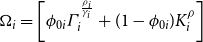 $\Omega _{i}=\left [\phi _{0i}\varGamma _{i}^{^{\frac {\rho _{i}}{\gamma _{i}}}}+(1-\phi _{0i})K_{i}^{\rho }\right ]$
and
 $\varGamma _{i}=\left [\theta _{0i}^{LH}\left (\frac {LHi}{LH_{0i}}\right )^{\gamma i}+\theta _{0i}^{LM}\left (\frac {LMi}{LM_{0i}}\right )^{\gamma i}+\left (1-\theta _{0i}^{LH}-\theta _{0i}^{LM}\right )\left (\frac {LLi}{LL_{0i}}\right )^{\gamma i}\right ].$
We opt for sector-country-specific averages of
 $Y$
,
 $K$
,
 $H$
,
 $LH$
,
 $LM$
, and
 $LL$
as normalization points in our exercise. This rationale follows Klump et al. (Reference Klump, McAdam and Willman2007), who argue that appropriate values for the distribution parameter are best detected from the data and that averages also net out short-term fluctuations.Footnote
14
4. Data and calibration
4.1 Output and input data
All output and input data used in this study come from the Socio-Economic Accounts in the World-Input-Output Database (WIOD-SEA).Footnote 15 The WIOD-SEA database has been constructed on the basis of national accounts data and harmonization procedures were applied in order to ensure international comparability. For the period 1995–2007, WIOD-SEA contains annual data for 35 industries in 40 countries (27 EU countries and 13 other major countries) on gross output and intermediate inputs at current basic prices, capital stock, as well as hours worked and labor compensation by skill type (low-, medium-, and high-skilled) (Timmer et al. Reference Timmer, Dietzenbacher, Los, Stehrer and Vries2015). Since information on the latter is not available at the industry level for a large number of countries, we aggregate the 35 industries into 14 sectors. Moreover, we drop the Mining and Quarrying sector as well as Public Utilities sector because they are unlikely to absorb large quantities of workers in reality, irrespective of their (marginal) labor productivities. The motivation to do so is that both sectors have high labor productivity levels, but are unlikely to absorb large quantities of workers in reality. This would considerably inflate the estimated (hypothetical) reallocation gains. The final sample therefore consists of the 12 sectors listed in Table 1.
Sector overview

Table 1. Long description
Table with columns for abbreviations, sector names, and ISIC Rev 3.1 descriptions. The abbreviations include AtB, D, F, G, H, I, J, K, L, M, N, and OtP. The sectors listed are Agriculture, Manufacturing, Construction, Trade Service, Hotels & Restaurants, Transport & Storage, Finance Services, Business Services, Public & Social Services, Education, Health & Social Work, and Other Services. Each sector has a corresponding description based on ISIC Rev 3.1.
A central issue for cross-country comparison of output and productivity levels is that output is expressed in international purchasing power parities (PPP). To account for the substantial variation in relative prices across industries, we use multilateral industry-level PPPs from Inklaar and Timmer (Reference Inklaar and Timmer2014) (see Table A.2 in the online appendix). As no information on relative prices are available for Taiwan, the sample reduces to 39 countries. Also, relative price data is only available for the year 2005. We therefore proceed as follows. We deflate both gross output and inputs using the industry-level price deflators integrated in WIOD-SEA and obtain growth rates of both series. An advantage of the double-deflated value-added method, compared to a single-deflated value-added measure, is that it can account for changes in the relative prices of intermediate inputs to gross outputs. The real growth rates are then used to extrapolate the gross output and intermediate input series, which are converted into PPPs for the available year 2005.Footnote 16 In a last step, we construct a value-added series in constant 2005 PPPs by subtracting the value of intermediate inputs from gross output, both in constant PPPs. For the physical capital stock, we use growth rates from the real capital stock data measured in national currencies in WIOD-SEA and the exchange rate from PWT 8.1 (Feenstra et al. Reference Feenstra, Inklaar and Timmer2015) to convert the series into constant 1995 US$.
The data on hours worked in WIOD-SEA includes both self-employed and employees.Footnote
17
Worker skill types are classified on the basis of educational attainment levels as defined in the International Standard Classification of Education (ISCED): low-skilled (ISCED categories 1 and 2), medium-skilled (ISCED 3 and 4), and high-skilled (ISCED 5 and 6). We define the general normalized human capital input in country
 $c$
in sector
 $i$
as L
 \begin{equation} \left (\frac {H_{ci}}{H_{0ci}}\right )^{{{\gamma }}_{ci}}=\left [\theta _{0ci}^{LL}\left (\frac {LL_{ci}}{LL_{0ci}}\right )^{{{\gamma }}_{{ci}}}+\theta _{0ci}^{LM}\left (\frac {LM_{ci}}{LM_{0ci}}\right )^{{{\gamma }}_{{{ci}}}}+\theta _{0ci}^{LH}\left (\frac {LH_{ci}}{LH_{0ci}}\right )^{{{\gamma }}_{{{ci}}}}\right ]^{\frac {1}{{\gamma{ci}}}} \end{equation}
where the subscript
 $0$
indicates the normalization point defined as the average over the period 1995–2007. Recall that both the Cobb–Douglas and the standard two-factor CES production function implicitly assume
 $\gamma =1$
(i.e., perfect substitutability of skill types at fixed ratios), in which case equation (20) can be rewritten as
 \begin{equation} \frac {H_{ci}}{H_{0ci}}=\theta _{0ci}^{LL}\times \left [\frac {LL_{ci}}{LL_{0ci}}+\frac {\theta _{0ci}^{LM}}{\theta _{0ci}^{LL}}\frac {LM_{ci}}{LM_{0ci}}+\frac {\theta _{0ci}^{LH}}{\theta _{0ci}^{LL}}\frac {LH_{ci}}{LH_{0ci}}\right ] \end{equation}
Further, note that the general normalized form in (21) includes the implicitly normalized human capital input
 $H_{ci}$
if
 $H_{0ci}=LL_{0ci}=LM_{0ci}=LH_{0ci}=1$
. In this case,
 $\theta _{0ci}^{LL}$
,
 $\theta _{0ci}^{LM}$
, and
 $\theta _{0ci}^{LH}$
collapse to measures of relative wages.Footnote
18
The general normalized human capital input thus incorporates the standard human capital input measured as unskilled worker equivalents with different worker types being weighted by their relative wage. Importantly, however,
 $\frac {H_{ci}}{H_{0ci}}$
also contains
 $\theta _{0ci}^{LL}$
, which measures the contribution of low-skilled workers to human capital services in sector
 $i$
in country
 $c$
.Footnote
19
In growth or development accounting exercises,
 $\theta _{0ci}^{LL}$
is often (implicitly) assumed to be fixed across time or equal across countries and can therefore be ignored (see, e.g., Jones Reference Jones2014).Footnote
20
Conversely, by working with the nested CES function in equation (19) directly, we implicitly assume that
 $\theta _{0ci}^{LL}$
differs across sectors and countries. Considering
 $\theta _{0ci}^{LL}$
in equation (21) is thus important to ensure consistency, and therefore, allow a direct comparison between the obtained cost of misallocation based on the different specifications.
4.2 Distribution parameters
Aside from output and input data, we need values for the distribution parameters. Since WIOD-SEA contains information on labor compensation at the sector level, we calibrate
 $\phi _{0ci}$
as the geometric average labor share in value added (measured in current prices in national currency) in sector
 $i$
in country
 $c$
over all time periods
 $T$
. This approach is common in the context of normalized CES production functions. Notably, WIOD-SEA also provides information on the compensation shares for each skill type. This allows us to further calculate
 $\theta _{0ci}^{LM}$
, and
 $\theta _{0ci}^{LH}$
based on the relative skill-shares in total labor compensation of each skill type working in sector
 $i$
in country
 $c$
at the normalization point. Specifically, we calculate
 \begin{align} \theta _{0ci}^{LH}=\left [\frac {\bar {w}_{ci}^{LH}\bar {LH_{ci}}}{\bar {w}_{ci}^{LL}\bar {LL_{ci}}+\bar {w}_{ci}^{LM}\bar {LM_{ci}}+\bar {w}_{ci}^{LH}\bar {LH_{ci}}}\right ] \\[-8pt] \nonumber \end{align}
 \begin{align} \theta _{0ci}^{LM}=\left [\frac {\bar {w}_{ci}^{LM}\bar {LM_{ci}}}{\bar {w}_{ci}^{LL}\bar {LL_{ci}}+\bar {w}_{ci}^{LM}\bar {LM_{ci}}+\bar {w}_{ci}^{LH}\bar {LH_{ci}}}\right ] \\[-8pt] \nonumber \end{align}
 \begin{align} \theta _{0ci}^{LL} =1-\theta _{0ci}^{LM}-\theta _{0ci}^{LH} \qquad\qquad \qquad \\[12pt] \nonumber \end{align}
where the bars indicate geometric averages over time.
Despite the effort put into the construction of WIOD-SEA, important limitations exist and warrant discussion. It is a well-known problem that hours worked and labor income of self-employed is not registered in the National Accounts in many countries. As discussed in detail in online appendix B, WIOD-SEA addresses this issue through imputation. A drawback of this imputation is that it can result in economically unreasonable labor revenue shares. Indeed, in 16 out of the 486 country-sector observations,
 $\phi _{0ci}$
exceeds the value of 1. We deal with these questionable parameter values in the baseline counterfactual by setting the maximum value of
 $\phi _{0ci}$
to 0.9. Admittedly, this ad hoc adjustment is somewhat arbitrary. We therefore run robustness tests, where we treat
 $\phi _{0ci}$
as a structural parameter that is common across countries.Footnote
21
It is worth noting that the relative efficiency parameters of skill types,
 $\theta _{0ci}^{LM}$
and
 $\theta _{0ci}^{LH}$
, are unaffected by a potential bias in
 $\phi _{0ci}$
as long as there is no systematic relation between compensation shares and self-employment.Footnote
22
4.3 Elasticity of substitution parameters
Lastly, we require values for the unobserved substitution parameters,
 $\sigma$
and
 $\eta$
. While there is now a large set of estimates for the aggregate elasticity of substitution between physical and human capital, evidence for the sector level is scarce. Also, the few available estimates do not directly map to the sectors considered in this paper. A secondary contribution of this paper is thus to estimate elasticities of substitution on the sector level that can then be used in the reallocation exercise. More precisely, we identify the parameters based on a normalized supply-side system of equations (Klump et al. Reference Klump, McAdam and Willman2007; Herrendorf et al. Reference Herrendorf, Herrington and Valentinyi2015; McAdam and Willman Reference McAdam and Willman2018). As shown by León-Ledesma et al. (Reference León-Ledesma, McAdam and Willman2010), this approach is superior to single-equation estimation or factor-demand-equation systems, as it not only increases the degrees of freedom but also considers both technology (via the underlying production function) and optimization behavior (via FOC equations).
Despite the advantages of the normalized system approach, identifying two elasticities simultaneously in a highly nonlinear function remains challenging. The identification is further constrained by the fact that the harmonized sector data in WIOD-SEA only cover a rather short time horizon. Against this background, we focus on the estimation of
 $\sigma$
, which we assume to differ across sectors, but not across countries and time. To consider the impact of
 $\eta$
on
 $\sigma$
, we follow a grid search approach as proposed by Henningsen and Henningsen (Reference Henningsen and Henningsen2012). That is, we impose plausible estimates of
 $\eta$
that are motivated by the literature and obtain corresponding estimates for
 $\sigma$
.Footnote
23
While clearly restrictive, note that these assumptions are implicitly also in use in all misallocation studies based on Cobb–Douglas, as this function implies
 $\sigma =1$
and
 $\eta \rightarrow \infty$
(see, e.g., Vollrath Reference Vollrath2009; Hsieh and Klenow Reference Hsieh and Klenow2009; Inklaar et al. Reference Inklaar, Lashitew and Timmer2017). Nonetheless, as a sensitivity test, we follow a more agnostic approach with regard to the true values of
 $\sigma _{ci}$
and
 $\eta _{ci}$
and compute bootstrap confidence intervals for
 $R_{c,USA}$
and
 $R_{World}$
.Footnote
24
Estimates of
 $\sigma$
.

For matter of space, the estimation specification of the normalized supply-side system and additional results are placed in online appendix E. The approach follows Trenczek and Wacker (Reference Trenczek and Wacker2026). Table 2 presents sector-specific estimates of
 $\sigma _{i}$
and corresponding 90%-confidence intervals (CI) based on bootstrap standard errors. Figure 2 additionally plots these estimates for
 $\eta \rightarrow \infty$
. Three findings stand out. First, in all sectors, and regardless of the imposed value of
 $\eta _{i}$
,
 $\sigma _{i}$
is estimated to be statistically significant below unity. Second,
 $\sigma _{i}$
is lower for lower values of
 $\eta _{i}$
and approximates the estimated value of the 1-level CES specification for
 $\eta \rightarrow \infty$
. Third,
 $\sigma _{i}$
is estimated quite precisely.
Sector elasticities of substitution with 90%-CI in parentheses

Table 2. Long description
A table comparing sector elasticities of substitution with 90%-confidence intervals for different values of eta. The table has 12 rows and 6 columns. Column headers are 2-Level CES with eta values of 1.6, 2, 4, 100, and 1-Level CES (implicit eta of infinity). Row labels are sector names including Agriculture, Manufacturing, Construction, Trade, Hotels & restaurants, Transport & storage, Financial intermediation, Business services, Public & social services, Education, Health & social work, and Other services. Each cell contains a value with a 90%-confidence interval in parentheses. Notable trends include varying elasticities across sectors and eta values, with some sectors showing higher elasticities at higher eta values.
Notes: Estimates of
 $\sigma$
(i.e., the elasticity of substitution between physical capital and the labor input aggregate with three skill types) based on different imposed values of
 $\eta$
. Estimation applies a two-step feasible nonlinear seemingly unrelated regression on a normalized supply-side system. 90%-CI in parentheses. Standard errors are bootstrapped based on 500 iterations.
There is some evidence to which we can compare these estimates, which are exactly in line with Chirinko (Reference Chirinko2008), but most of this evidence is restricted to the USA. For instance, Young (Reference Young2013) finds that the elasticity of substitution between physical and human capital is less than unity for a large majority of US 2-digit SIC level industries. Aggregating industries into sectors based on value-added-share-weights, Young (Reference Young2013) obtains an elasticity of 0.57 in the manufacturing sector and of 0.66 in services. Using capital price series and applying a low-pass filter to better capture the long-run substitution elasticity, Chirinko and Mallick (Reference Chirinko and Mallick2017) find industry-level estimates for USA to be below unity with most estimates being in a range of 0.2–0.7. Similar estimates are also found by Dissou et al. (Reference Dissou, Karnizova and Sun2015) in ten Canadian manufacturing industries for the period 1962–1997 and by Oberfield and Raval (Reference Oberfield and Raval2021), who recover elasticities for two-digit SIC US industries from plant-based estimates. The latter estimate a weighted average plant-level elasticity of 0.52 in manufacturing. Taking substitution across plants and industries into account, they recover an aggregate elasticity of 0.75 for the manufacturing sector in 2007. For broad sectors, Herrendorf et al. (Reference Herrendorf, Herrington and Valentinyi2015) find that capital and labor are gross complements in US manufacturing and services. Conversely, they estimate an elasticity of above one in agriculture. This stands in contrast to Mundlak’s (Reference Mundlak2005) examination of the US agriculture sector, advocating an elasticity of equal or below 1.Footnote 25 ? also finds that labor and traditional capital are gross complements in sector-level EU KLEMS data. Overall, the sector estimates for the elasticity of substitution between physical capital and the human capital aggregate obtained in this paper seem to be fairly consistent with previous findings. Moreover, the estimates strongly suggest substitution elasticities that are inconsistent with Cobb–Douglas and in favor of a more flexible CES specification. It should finally be emphasized that long-run elasticities are usually higher than short-run elasticities (León-Ledesma and Satchi Reference León-Ledesma and Satchi2018; Koh and Santaeulalia-Llopis Reference Koh and Santaeulalia-Llopis2022).
5. Counterfactual results
Equipped with the parameter values, we can now calculate the hypothetical output per worker level for each country,
 $y_{c}^{H^{*}}$
, that would be implied by an optimal allocation of human capital across as defined in (18). Based on
 $y_{c}^{H^{*}}$
, we can then obtain the ratio
 $R_{World}$
. A central result of this paper is depicted in Figure 3, which shows values of
 $R_{World}$
for three different specifications. For now, we will focus on specifications that assume perfect substitutability between different skill types of workers (HC) with associated efficiency weights and the final year 2007.
The benchmark result of
 $R_{World} = 0.79$
obtained under the commonly used Cobb–Douglas setup with human capital as labor input (CD-HC in in Figure 3) suggests that 21% of the cross-country output per worker variation can be explained by differences in the efficiency of human capital allocations across sectors within countries. This share reduces by 6 percentage points to 15 percent if we assume sectors to be characterized by a CES function and impose the estimated sectoral elasticities of substitution (CES-HC). In other words, the share of output per worker differences across countries that can be explained by human capital misallocation is more than one fourth less under the empirically more plausible CES production function than under the Cobb–Douglas function that is commonly used in the literature. To further put this into perspective: the quantitative difference in results between both functional forms (top two points in Figure 3) is similar to the difference in accounting or not accounting for skill levels of workers in the Cobb–Douglas case (bottom two points in Figure 3; 0.74 for CD-EMP assuming raw hours worked as labor input).
To better understand what drives these results, we look at the individual country results (see also subsection 5.2). Table 3 presents summary statistics for the year 2007. The first row presents results for a simple labor input measured in raw hours worked. On average, output per worker increases by about 12.8 % if countries allocate labor efficiently across sectors. The large spreads between the respective percentiles and the large gap between the mean and median indicate, however, that countries record sizable differences in their current misallocation costs. We replace the simple labor input with a measure of human capital in row (2). In line with previous findings, the hypothetical gains decrease (to 10.6 %). This indicates that some of the apparent misallocation of labor across sectors can be explained by cross-sector differences in human capital (Gollin et al. Reference Gollin, Lagakos and Waugh2014; Vollrath Reference Vollrath2014; Herrendorf and Schoellman Reference Herrendorf and Schoellman2018).
Gains from reallocation of human capital (2007)

Table 3. Long description
A table comparing gains from reallocation of human capital in 2007 across different percentiles and specifications. The table has 3 rows and 8 columns. The columns are labeled Percentile, Min, 10th, 25th, Median, Mean, 75th, 90th, and Max. The rows are labeled CD-EMP, CD-HC, and CES-HC. Row 1: CD-EMP, 2.4, 3.5, 4.3, 6.0, 12.8, 9.9, 22.5, 141.2. Row 2: CD-HC, 1.2, 3, 3.5, 5.6, 10.6, 9.8, 17.9, 105.3. Row 3: CES-HC, 0.8, 2.2, 2.8, 4.2, 7.6, 8.5, 16.4, 65.9.
Note: Hypothetical output per worker gains in percentage points. Calculation based on different specifications of normalized sector production functions. Specifications: EMP: Labor input measured in raw hours worked. HC: Labor input measured as quality adjusted hours worked. CD: Cobb–Douglas production function. CES: Constant elasticity substitution function. All calculations based on value added measured in PPPs for 12 sectors.
Baseline results for
 $R_{World}$
.
Note: Own calculation based on WIOD-SEA.
 $R_{World}$
states the remaining fraction of output per worker variation after misallocation across sectors is eliminated. Specifications: CD: Cobb–Douglas production function. CES: Constant elasticity substitution function. EMP: Labor input measured in raw hours worked. HC: Labor input measured as quality adjusted hours worked. All calculations based on value added measured in constant PPPs for 12 sectors.

Most important for this paper is the change in the distribution of the reallocation gains when we depart from the assumption of an unitary elasticity of substitution between physical and human capital. Row (3) shows that the average gains decrease to 7.6% and are smaller than in the Cobb–Douglas case at each percentile. At the mean (median), human capital reallocation gains are 28 (25) % lower under the more plausible CES production structure.
What drives the reduction of reallocation gains in the CES case? Recall that our estimates impose substitution elasticities of below unity, which implies that the physical and human capital are gross complements in all sectors. As a consequence, marginal products respond more strongly to changes in human capital allocation across sectors. A laborer moving from a low-productivity sector A to a high-productivity sector B initially experiences a strong increase in marginal productivity: since human capital is scarce in sector B and physical capital
 $K$
is relatively abundant, the laborer is using this capital in sector B very productively when
 $H$
and
 $K$
are complements. Since we only focus on the reallocation of human capital and consider physical capital fixed in each sector, this effect quickly decays: there is not enough physical capital
 $K$
available in sector B that a large influx of laborers could work with.Footnote
26
This results in faster convergence of the marginal products across sectors, leading to less reallocation, and lower output growth overall.Footnote
27
To what extent these differences affect the ratio
 $R_{World}$
depends on whether the country gains respond differently to the production function specification and whether this variation is correlated with output per worker. Figure 4 sheds light on this issue. The figure shows each country’s value of
 $R_{USA}$
for different specifications in relation to their output per worker. Recall that
 $R_{c,USA}$
states the remaining output per worker gap of a country relative to the USA after differences in labor allocation efficiency across sectors have been removed, effectively normalizing the hypothetical gains across countries. While many countries seem to not differ too much in their degree of misallocation, those countries that do have large efficiency losses tend to be at the poorer end of the output per worker distribution. In fact, two of the three poorest countries, India and China, have, by far, the largest reduction in the output gap to the USA. It is further noticeable that while not all countries are estimated to have a lower efficiency gap relative to the USA in a CES setup, this does seem to be the case for all countries in the lower half of the distribution. For instance, eliminating differences in human capital misallocation across sectors reduces the output gap to the USA in the year 2007 for India (China) by 48% (33%) in the case of Cobb–Douglas, but only by 34% (17%) under the CES specification.
Baseline results for
 $R_{USA}$
.
Note: Own calculation based on WIOD-SEA. CD: Cobb–Douglas production function. CES: Constant elasticity substitution function with sector-specific
 $\sigma _{i}$
. All calculations based on value added measured in constant PPPs for 12 sectors; output per worker is denominated in thousands.

5.1 Imperfect skill substitution
We now relax the implicit assumption that labor skill types are perfect substitutes (at fixed ratios). That is, we now rely on the nested CES production function (8) instead of the simple CES production function (6) and on the associated optimal allocation defined in (19) instead of (18).
Table 4 summarizes the hypothetical gains for the nested CES specifications. Rows (1)–(3) still impose
 $\sigma _{i}$
to be unity, while rows (4)–(6) consider different values of
 $\eta _{i}$
and a simultaneous change in the corresponding
 $\sigma _{i}$
. Some changes in the distributions are visible. However, if we fix
 $\sigma _{i}$
, the reallocation gains change only marginally for different values of
 $\eta _{i}$
, with notable exceptions in the case of India and Romania (see online appendix Figure A.1). Overall, the results suggest that the substitutability of physical capital and the human capital aggregate has larger quantitative implications than relaxing the assumption of perfect substitution (at fixed ratios) across skill types. This aligns with the finding of Hendricks and Schoellman (Reference Hendricks and Schoellman2023) that imperfect substitution of skills has limited consequences for cross-country output differences.
Gains from reallocation (other specifications, 2007)

Table 4. Long description
A table comparing hypothetical output per worker gains in percentage points across different specifications. The table has 6 rows and 8 columns. Column headers are Percentile, Min, 10th, 25th, Median, Mean, 75th, 90th, Max. Row labels are (1) to (6). Row 1: Percentile, Min, 10th, 25th, Median, Mean, 75th, 90th, Max. Row 2: (1), 2.0, 3.2, 3.7, 6.0, 10.5, 9.5, 18.6, 92.6. Row 3: (2), 1.9, 3.1, 3.6, 5.6, 10.0, 9.0, 17.5, 85.0. Row 4: (3), 1.8, 3.1, 3.5, 5.6, 9.8, 8.9, 17.3, 82.0. Row 5: (4), 1.4, 2.4, 3.1, 4.2, 7.3, 7.9, 14.3, 55.6. Row 6: (5), 1.3, 2.3, 2.8, 3.9, 6.9, 7.4, 13.2, 51.8. Row 7: (6), 1.3, 2.3, 2.8, 3.8, 6.8, 7.3, 13.0, 50.5.
Note: Hypothetical output per worker gains in percentage points. Calculation based on different specifications of normalized sector production functions. Note that
 $\eta$
is assumed homogeneous across sectors and determines
 $\sigma$
in the 2-level nested CES function in rows (4)–(6). All calculations based on value added measured in PPPs for 12 sectors.
5.2 Comparison to prior studies and capital mobility
There is limited evidence to which we can compare our estimates, as studies differ in their focus regarding input factors (physical and/or human capital), aggregation level (sector, industry, or firm), or outcome measure (TFP or output). It is thus informative to note that absolute reallocation gains would increase in our CES framework if we also allow for mobility of physical capital across sectors. In this case, capital would follow labor to more productive sectors and thus slows down the decline in labor’s
 $MPV$
.Footnote
28
The seminal study by Hsieh and Klenow (Reference Hsieh and Klenow2009) calculates that improving factor allocation across firms to the extent observed in the United States could raise manufacturing productivity by 30–50% in China and 40–60% in India. Our exercise suggests aggregate gains from human capital reallocation of 58% (27.1%) for China and 105% (66%) for India in the Cobb–Douglas (CES) case. Yet, our study differs by the level of analysis (sector vs. firms), coverage (all sectors vs. within manufacturing; year), and factor mobility (human capital vs. labor and capital). Provided that productivity differences across sectors are large, especially in lower-income countries, and our counterfactual achieves full allocative efficiency of human capital (not just US efficiency), we consider our magnitudes for those two countries highly plausible despite the fact that keeping physical capital fixed provides a short-run lower bound of reallocation gains.
Inklaar et al. (Reference Inklaar, Lashitew and Timmer2017) estimate that the average observed manufacturing productivity level in their sample of 52 medium- and low-income countries would rise from 23% to 37% of the US level if cross-country differences in both capital and labor misallocation would be eliminated. This implies a 61% increase, which seems a bit high compared to our resultsFootnote 29 but not implausible in overall magnitude, considering that our study differs in the sample composition, level of analysis, factor mobility etc.
Closer to our study, Vollrath (Reference Vollrath2009) estimates that variation across countries in the degree of human capital misallocation between the agriculture and non-agriculture sector could account for 30% of the variation in income per capita in his sample of 42 countries. Considering that Vollrath only looks at efficiency losses that occur between agriculture and the remainder of the economy, this estimate appears to be large, but it does not necessarily contradict ours. For one, Vollrath’s sample consists of several economies in which the agriculture sector employs a large share of total human capital and where the marginal product gaps of human capital between agriculture and industry are large (see Table 2 in Vollrath Reference Vollrath2009). This suggests that human capital misallocation can possibly explain a substantial part of output per worker differences in his sample. Moreover, Vollrath is forced to work with an arguably cruder sectoral measure of human capital. These differences considered, Vollrath’s empirical estimates are not inconsistent with our findings.
6. Robustness and extensions
6.1 Robustness
6.1.1 Parameter assumptions
Until now, we have not only assumed that
 $\sigma _{i}$
and
 $\eta$
are homogeneous across countries, but we have also imposed a common
 $\eta$
for all sectors. To test how sensitive our results are to these assumptions, we artificially introduce variation in the substitution parameters. Specifically, we perform 1,000 calculations of
 $R_{World}$
and
 $R_{c,USA}$
based on simulated samples. For each sample, we draw random values for
 $\eta _{ci}$
from the possibility set
 $[1.6,\,2,\,4,\,\infty ]$
. For a given
 $\eta _{ci}$
, we then obtain the corresponding
 $\sigma _{ci}$
from the 90%-CI around
 $\hat {\sigma }_{i}(\eta _{i})$
.Footnote
30
The motivation for this simulation is as follows. Provided that the actual degree of cross-country parameter heterogeneity is moderate, in the sense that the 90%-CI envelops most of the true parameter values in each country and sector, increasing the set of possible production structures also raises the probability of approximating the true production side.
Figure A.5 in the online appendix shows the 10th-to-90th percentile from the resulting distribution of
 $R_{World}$
. Two findings stand out. First,
 $R_{World}$
reacts rather sensitively to variation in
 $\eta _{ci}$
and
 $\sigma _{ci}$
(about 3–4 percentage points). Second, departing from the Cobb–Douglas assumption reduces the fraction of output per worker variation explained by misallocation by at least 6 percentage points. Figures A.6 and A.7 in the online appendix show the 10th-to-90th percentile interval of each country’s hypothetical gains and remaining gap to the USA, respectively. Countries are ordered by their actual output per worker. The figures indicate that for many countries the estimated reallocation gains are robust to the artificial variation in
 $\eta _{ci}$
and
 $\sigma _{ci}$
. Nevertheless, there are several countries, especially in the lower half of the output per worker distribution in the sample, for which the estimated absolute (and relative) gains from reallocation are sensitive to the imposed parameter values.
So far, the results are based on production functions with a distribution parameter
 $\phi _{0ci}$
specific to each country and sector. As a robustness test, we replace
 $\phi _{0ci}$
by a structural parameter that is common across countries. Figure A.8 in the online appendix shows the results for
 $R_{World}$
. Noticeable, the cross-country differences in the estimated efficiency losses increase when we treat the distribution parameter
 $\phi _{0i}$
as structural and are largest if we impose the distribution parameter obtained for the USA,
 $\phi _{0USAi}$
, as the true technology parameter for all countries. In this case, the Cobb–Douglas results suggest that differences in human capital misallocation explain as much as 28% of the output per worker variation in 2007.
The explanation for this is visible in Figure A.9 of online appendix A. With imposed
 $\phi _{0USAi}$
in all countries, countries in the lower half of the income distribution obtain larger hypothetical gains from reallocation relative to the USA. Put differently, countries are estimated to be less inefficient in allocating their human capital across sectors if technology parameters are assumed to be country-specific.Footnote
31
This seems economically plausible and possibly reflects that firms (and countries) opt for technologies that are appropriate for their factor endowments (see, e.g., Caselli Reference Caselli2005).
In terms of sensitivity regarding
 $\eta _{ci}$
and
 $\sigma _{ci}$
, the 10th-to-90th inter-percentile range spans from 0.79 to 0.83. This implies that human capital misallocation explains between 17% and 21% of the output per worker variation, given that
 $\phi _{0USAi}$
resembles the true technology parameter in all countries. Overall, the robustness exercises regarding the assumed parameter values support the previous finding that imposing a Cobb–Douglas production function specification can have sizable implications for the estimated gains from reallocation. It does, however, not necessarily have to. The appropriateness and quantitative implications of the production function specification should therefore be evaluated on a case-by-case basis.
6.1.2 Sample composition and non-market services
We have found that countries differ not only in their degree of human capital misallocation, but also by how much their estimated hypothetical gains differ across production function specifications. This raises the question to what extent the change in
 $R_{World}$
across specifications is robust to the sample composition. To examine this, we create 1,000 simulated samples consisting of 100 countries drawn with replacement from the original set of 39 countries in our sample. For each sample, we calculate
 $R_{World}$
based on the Cobb–Douglas and CES specification. Figure A.10 in the online appendix plots the difference in
 $R_{World}$
between the two specifications. The 10th and 90th percentile lines mark a difference of 4 and 8 percentage points, respectively. If we set this into relation to the 6 percent difference from the baseline, this indicates that the previous result is moderately sensitive to the countries in the sample.
Evidence on how sensitive the absolute value of
 $R_{World}$
is to the sample composition is shown in Figure A.11 of online appendix A, which depicts the respective distributions and means of
 $R_{World}$
for different specifications. Two things are noticeable. On the one hand, there is a considerable degree of variation in
 $R_{World}$
for each specification, and as a consequence, overlap across the different specifications. On the other hand, there is a noticeable differences in the distributions. This indicates that the previous finding that the Cobb–Douglas specification overstates the role of misallocation in explaining output per worker variation is not just an artifact of the sample composition. Section 6.1.3 of the working paper version of our paper additionally provides a robustness check without the non-market services sectors (which may be poorly measured; Trenczek and Wacker Reference Trenczek and Wacker2025).
6.1.3 Small open economy extension with fixed prices
In equation (5) we assumed that the aggregate final good of the economy is produced by a Cobb–Douglas aggregate over all sectors. While this is consistent with the seminal benchmark in Hsieh and Klenow (Reference Hsieh and Klenow2009), it is certainly an assumption one may question. For example, in a small open economy, the prices of tradables are equal to world prices and invariant to domestic factor allocations. We hence also considered a reallocation exercise for the scenario of perfect substitution between sector outputs at fixed proportions (i.e., constant relative prices).
In this scenario, convergence in the value of the marginal product across sectors is achieved more slowly, resulting in more labor being shifted during optimization and larger overall gains from reallocation. The fact that one would expect this result under non-responsive prices adds to the plausibility of our approach. However, the quantitative magnitudes in this scenario are not necessarily realistic because tradeability is limited in reality. For example, in the case of Turkey we find that human capital drops dramatically in education and health, while construction expands to an implausible extent. But neither sector is characterized by high tradeability – complete specialization in construction cannot achieve education or health through imports. While this particular scenario of fixed prices may hence be unrealistic, it shows that the further investigation of alternative final good aggregators is a promising avenue for additional research.Footnote 32
6.2 Country dynamics in misallocation over time
One interesting finding depicted in Figure 3 is the stability in
 $R_{World}$
over the years. Figure A.12 in the online appendix indicates that this hides country dynamics in misallocation over time. The figure plots the hypothetical gains from reallocation for six countries. What we see is a mixed picture. Two countries, namely the Republic of Korea and the Czech Republic, improved the allocation of human capital across sectors over the 12 year period. On the contrary, in countries like Belgium, China, Greece, and India, the aggregate output costs of human capital misallocation in 2007 exceed the 1995 level. In light of the widespread structural change that occurred in China and India, this finding seems puzzling. However, underlying these developments are different records of human capital reallocation across sectors and productivity growth within sectors. While a thorough investigation is beyond the scope of this paper, it is worth noting that an increase in the aggregate costs of misallocation does not imply that there has been no growth-enhancing reallocation of workers across sectors over the period. In fact, in both China and India the reallocation of human capital across sectors contributed positively to growth, albeit just marginally (see online appendix table A.3).Footnote
33
The dominant contribution came from within sector productivity growth. In fact, in both countries, marginal productivity values of human capital in agriculture remained low, despite substantial reallocation. Conversely, marginal productivity values increased further in other sectors. Consequently, gaps in marginal products across sectors increased. Rapid productivity growth within highly productive sectors can thus increase allocative inefficiency.Footnote
34
At the same time, however, it raises the potential for growth-enhancing human capital reallocation.
7. Conclusion
In this paper, we have examined whether the strong functional form assumptions imposed by Cobb–Douglas functions have quantitatively important implications for measuring aggregate costs of human capital misallocation across sectors for a sample of 39 countries. We extend the misallocation framework to the CES and nested CES specification by drawing on a normalization approach. This allows suitable counterfactuals and facilitates estimation of sector-level substitution elasticities. Physical capital and the human capital input are estimated to be gross complements in all sectors. This suggests that counterfactuals based on Cobb–Douglas sector production functions are not appropriate.
We find that relaxing assumptions on the substitutability of input factors affects the hypothetical gains from reallocation considerably in some countries, but not in all. As a consequence, the degree to which human capital misallocation can explain aggregate output per worker variation in the sample drops from 21% (Cobb–Douglas) to 15% (CES). Allowing for imperfect substitution of skill types has by itself only small effects on the estimated reallocation gains. It does, however, imply some changes in the estimated elasticity of substitution between physical capital and the human capital aggregate, which in turn translate into moderate changes in the estimated reallocation gains. Finally, we find that the fraction of output per worker variation in the sample that can be explained by cross-country differences in the degree of human capital misallocation across sectors has been quite stable over the period 1995–2007. This stability, however, hides the fact that countries experienced different developments regarding the extent of cross-sector human capital misallocation.
Our results raise the question whether previous work has overestimated the role of factor misallocation by working with a Cobb–Douglas production function. Future research may scrutinize this issue. First, we have focused on the allocation of one production factor only, keeping the other production factor fixed. In the long run, physical capital may reallocate as well, leading to different quantitative implications (see subsection 5.2). Second, and relatedly, the rate at which marginal products of one production factor are equated across sectors or firms depends on how abundant or scarce the mobile factor is in the economy. Additionally, we want to emphasize that output gains from efficiently allocating human capital across sectors, which we estimate to be 7.6 % on average, are still substantial.
In any case, the results stress that the appropriateness and quantitative implications of the production function specification should be evaluated on a case-by-case basis. Hence, a test for model specification should be a prerequisite for parametric counterfactuals that gauge the aggregate cost of factor misallocation, irrespective of whether they focus on the macro or micro level. For cases in which the CES specification is found more appropriate, this paper presents an approach to extend the misallocation framework beyond Cobb–Douglas.
Supplementary material
The supplementary material for this article can be found at https://doi.org/10.1017/S1365100526101345.
Acknowledgements
We thank Francesco Caselli, Daniel Henderson, Ryo Horii, Maurizio Iacopetta, Beata Javorcik, Rainer Klump, Jakub Muck, and Chris Parmeter for beneficial discussions, two anonymous referees for their extremely thoughtful and useful suggestions, and scholars from Oxford, Osaka, Mainz, Heidelberg, Frankfurt, and Mannheim, as well as participants at the NAPWX Conference in Miami, the INFER Conference in Valencia, the TPI Conference in Manchester, and a Workshop on Dynamic Macroeconomics in Vienna for helpful comments and suggestions. Financial support from the Foundation of German Business (sdw) is gratefully acknowledged. This paper is based on the third chapter of Jan Trenczek’s dissertation “Essays on Structural Transformation”.


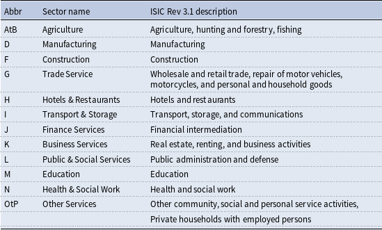
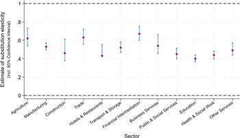
 σ
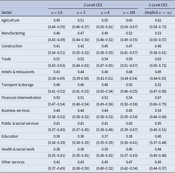
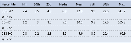
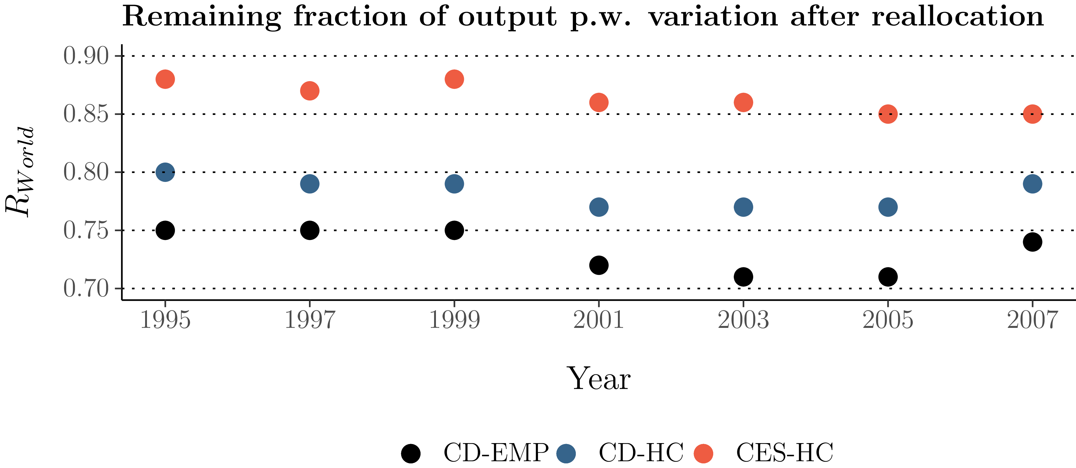
 RWorld
 RWorld

 RUSA
 σi
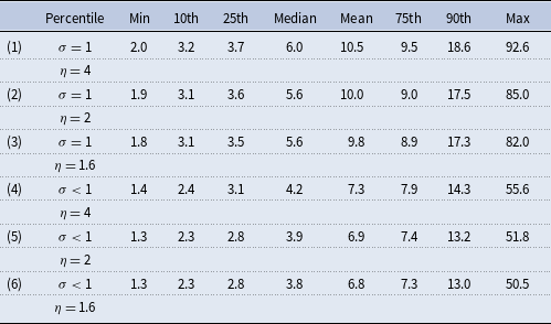


 Open access

