1 Introduction
The funding of pensions is an issue that has acquired particular relevance in recent years, due to the increased longevity of the population. Whatever the system adopted by a country, there will always be risks to mitigate. In the case of defined-benefit systems, the institution sponsoring the plan assumes the investment and longevity risks. Meanwhile, the workers assume the labor risk that may imply, in some cases, having no benefit at all, due to failure to meet the requirements, and in others, receiving very small benefits indeed. At the same time, there is the risk that the sponsor may find itself in a state of insolvency and be unable to fulfill its commitments. On the other hand, in a defined-contribution pension system, the investment and longevity risks are assumed by the members, during their active life at least, and additional to these are the risks associated with the labor market, among others. In the case of Chile, the defined-contribution pillar is the main source of retirement income provided by the pension system for a large number of people, and contribution to it is mandatory. In this context, insofar as the risk associated with investments made to finance the pension is concerned, the actual regulation offers five types of funds that differ in their investment strategy and associated risk. In the event of the member's not choosing a type of fund, a default allocation mechanism is assigned according to his/her age. In any case, the most aggressive option is restricted to people who are at least 10 years away from reaching legal retirement age. The modern financial theory has proposed that a suitable investment strategy for mitigating the risks in an individually funded system is to allocate assets in the portfolio according to the life-cycle profile of the individual, with exposure to risky assets decreasing over time toward a portfolio composed of less volatile assets at the point of retirement (see, e.g., Viceira, Reference Viceira2007). This strategy aims to minimize the risk associated with a sudden fall in the value of the pension at the very moment when the person ‘needs’ or has planned to start drawing a pension. Although the choice of an optimum investment strategy depends on individual characteristics, such as the degree of risk aversion, human capital, expected volatility of wages, work history, family composition and other sources of wealth; in practice the vast majority of the members of a pension system do not have sufficient knowledge to take a sensible decision with regard to the investment of their pension savings. This is true in any system, where there is abundant evidence that the scant level of financial knowledge makes it difficult for basic decisions to be taken, and biases occur such as choosing on the basis of the past performance of funds. Given the lack of financial knowledge and the evidence on inertia on decision making in terms of pension issues the design of default options is critical. This paper is a contribution toward providing a definition of the investment risks for pensions and an assessment of the impact of different investment strategies on expected pension and the pension risk. For this purpose, we analyze the probability density function (PDF) of replacement rates, and how this distribution changes on the basis of different investment strategies during the member's life cycle. The analysis considers potential differences among heterogeneous individuals by replicating the calculations for different representative individual profiles by gender, education and contribution density. Our results suggest that affiliates can expect a gain (loss) of around 0.85 percentage points in terms of average replacement rates in return for an increase (decrease) of 1 percentage point in risk, measured as standard deviation of replacement rates. Using a stochastic dominance analysis, we find that there are no dominated strategies when subsidies from the Solidarity Pillar are excluded. We view the lack of dominated investment strategies as a positive result, since it suggests that each type of fund should be attractive for affiliates with different risk tolerance. However, this also means that a more precise definition of the affiliates' utility function must be made in order to find the optimal investment strategy. We view this issue as relevant for the future work. We explore the impact that the existence of the Solidarity Pillar may have on the design of default investment strategies. Our results imply that the most appropriate investment strategies for affiliates that may qualify for this Pillar (i.e. affiliates with both low education and low density of contributions) are those which concentrate on riskier funds. However, it is important to bear in mind that any increase in the risk of the strategies could put more pressure on Government spending in order to grant additional benefits to affiliates. The methodology that is developed in this paper can be used to evaluate default options by regulators where we show that there would always be a tradeoff between the risk and expected replacement rates. Additionally, other components of the pension system that contribute to financing retirement should also be considered at moment of deciding on default options bearing in mind not only the impact on the level of total benefits but also the fact that risks might be transferred to the state, as it will be shown for the case of Chile. Therefore, the definition of a target replacement rate and a level of individual risk tolerance, as well as government risk tolerance, are needed for an adequate policy design in this regard. The next section discusses the role of life-cycle investment strategies as default allocations. Section 3 looks in more depth at the most appropriate way of measuring pension risk for an individually funded pension system, whereas Section 4 gives the results of simulations for different types of workers under different investment strategies. In this section, it is also assessed the role of the Solidarity Pillar in the case of Chile, as a way of sharing risks between individuals and the state, which can also be seen as a risk-sharing arrangement among different generations. Finally, Section 5 gives some conclusions and announces the future challenges.
2 Life-cycle investment strategies as default allocations
The existence of default allocations is relevant in a context where affiliates display little financial knowledge, and in particular scarce knowledge and understanding of the pension system in which they participate. In the case of Chile, the lack of financial knowledge was revealed in the Social Protection Survey. For instance,Footnote 1 82% of affiliates do not know how their pension will be calculated. Moreover, almost half from those who claim to know about this subject give an incorrect description. Additionally, almost 60% of affiliates have neither knowledge of the existence of different types of pension fund nor can they explain the differences among these funds. It should be noted that the lack of financial education is not unique to Chile. Indeed, Lusardi and Mitchell (Reference Lusardi and Mitchell2005) and Lusardi and Mitchell (Reference Lusardi and Mitchell2008) study the behavior of individuals with 50 or more years of age and find that there is a generalized lack of financial knowledge, especially among women, minorities and individuals with low levels of education. These authors conclude that the degree of financial knowledge is highly correlated with the lack of skills to plan for retirement and portfolio choice. In line with the lack of financial knowledge of Chilean affiliates, there is a high degree of inertia in investment decisions. Individuals fail to review past decisions and/or postpone investment decisions (e.g., they postpone saving, don't save or don't save enough). Another important factor that influences affiliates' decisions is the existence of myopic behavior, which manifests itself as high inter-temporal discount rates. Barr and Diamond (Reference Barr and Diamond2008) argue that individuals tend to seek short-term gratification, which translates, for instance in opting for early retirement even though this reduces the amount of pensions. Moreover, individuals avoid making explicit decisions (opt-in versus opt-out) which implies that mechanisms such as automatic enrollment generally produce higher participation rates. For the reasons described above, when there are alternative investment portfolios available for individuals to make a decision, the existence of a default option and it's characteristics are critical. In this respect, it must be considered that more aggressive retirement strategies imply not only a higher expected return but also a higher probability of a significant decrease in pension assets, thereby the exposure to risk when individuals are close to retirement could be less suitable since there is less time to recover from a sudden fall if it happens few years before retirement. Also, Viceira (Reference Viceira2007) argues conceptually that an individual's total wealth is made up of his financial wealth and human capital, the latter element being measured as the present value of his future income from work. Therefore, changes in the relative importance of these two sources of wealth over the course of an individual's life justifies the adoption of investment strategies in which the portfolio is gradually adjusted according to the worker's age (age-based strategies). At the beginning of the working life, it would be more appropriate to take risks in financial investment searching for higher returns. In this case, the human capital would act as an insurance mechanism since, assuming relatively constant labor income, this component may approximate to an implicit investment in bonds. When approaching retirement age, the objective changes to one of safeguarding financial wealth by investing in safer instruments. In this line of argument, the design of investment strategies of this type also should take the heterogeneity of the members into account. For some workers, it would be more plausible to assume that labor income is uncertain and might therefore not be similar to an implicit holding in bonds. The level of uncertainty in labor income will depend on the degree of correlation between wages and the economic cycle, the type of contract the worker has (open-ended or fixed-term) and his level of education, among other factors. On this line, Gomez et al. (Reference Gomez, Kotlikoff and Viceira2008) argue that for plausible values of wage volatility, it is still advisable to have an investment policy with decreasing amounts of variable income according to age, but selecting a more conservative portfolio for those individuals with more unstable jobs.Footnote 2 Additionally, other sources of pension income should be considered, for instance if the member qualifies to receive benefits from the state, subsidies and/or guarantees to make up his pension, a more aggressive investment strategy might be better for the individual, because obtaining such benefits would mitigate the risks associated with a portfolio more slanted toward equities. However, it must be noted that risks do not disappear, but are transferred to the Government in this case. Another relevant factor to consider is the degree of risk-tolerance, meaning that a well-defined set of strategies should include aggressive, intermediate and conservative options, to satisfy the various risk/return preferences of individuals. Even if it is agreed that a life-cycle approach is suitable, there is a whole range of alternatives paths. In order to assess how different investment strategies affect risk in a defined-contribution pension system, it is necessary to have an adequate measurement of risk that includes all the relevant factors that may affect an individual's pension. Section 4 assesses the impact on pensions of different life-cycle options in the case of Chile, between which the current default is included.
3 Pension risk model
In order to be able to measure the pension risk associated with different investment strategies, a simulation exercise has been carried out. This exercise includes the characteristics of the Chilean pension system as well as the characteristics of the Chilean labor market. The outcome of the simulations are the estimation of expected replacement rates associated with different investment strategies, as well as the PDF of these replacement rates to have an assessment of pension risk. In the next subsections, we define the appropriate risk measure for a DC pension system. It is important to note that this metric is different from measures of short-term volatility commonly used by the financial industry.
3.1 Short-term volatility versus pension risk
Having a reliable measurement of pension risk is not an easy task. For example, the short-term volatility of the pension funds' return is not necessarily a good indicator of the pension risk in the case of a member who is at the beginning of his/her active working life and is still 30 years away from retirement. In light of this, it is necessary to concentrate on the considerations needed to have a pension-risk definition that makes sense. The financial literature has analyzed and suggested various quantitative tools for measuring risk, but these generally present serious limitations when it comes to evaluating their use in measuring the risk of the pension system. The application of VaR models, for example, might be an attractive alternative. It is an instrument in widespread use in the financial sector as a measure of market risk and is easy to interpret. However, it has one important limitation: it has a short-term approach which is not appropriate for measuring long-term investment strategies such as is the case of the pension funds.Footnote 3 Besides, it is necessary to define an appropriate variable on which to measure pension risk, one that includes all relevant sources of risk faced by members of the pension system: contribution-density risk or the risk of becoming unemployed; the funds' investment risk; and the risk of annuitization or re-investment, when the final balance of the member's individual account is transformed on retirement into the value of the pension. Bearing in mind the long-term nature of the pension funds and the aforementioned risks associated with the pension, pension risk must be measured and evaluated from the point of view of the contributor's life cycle. Consistent with this objective, the target variable that best represents the member's position on retirement is the replacement rate, measured as the ratio between the value of the pension at the moment of retirement and a relevant measurement of wage. What we are definitely interested in analyzing is the PDF of the replacement rate, and how this distribution changes on the basis of different investment strategies during the member's life cycle. Conceptually, the appropriate measurement of risk is given by the marginal effect on the expected replacement rate of carrying out a particular investment strategy, the scatter around that expected value and the shape of its density function. In the next subsection, we analyze the database and methodology used to estimate the PDF of the replacement rate. That methodology provides us with the appropriate tool for correctly evaluating the impact on expected pensions and volatility of following different investment strategies, and particularly life-cycle strategies.
3.2 Methodology
In this subsection, we give a detailed description of the model used to measure pension risk. The model has an income and contributions module in which we estimate the life-cycle paths for labor income and probability of contribution to the pension system for different types of representative individuals. We also model human capital risk and financial markets risk. With these elements we are able to produce a final account balance at the age of retirement, which is then annuitized to estimate a pension and a replacement rate.
3.2.1 Income profiles
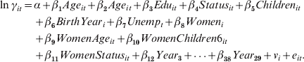
The pension obtained at retirement is determined by the contributions that members pay into the system. Those contributions in turn are determined by members' job characteristics, labor stability, timing and duration of unemployment spells in their working life, among other variables. This paper uses a unique data set that combines administrative data from the Historias Previsionales de Afiliados Database (HPA) with a survey, Encuesta de Protección Social (EPS 2009), conducted on the same individuals. The HPA contains administrative records of every contribution made by individuals in the representative sample. This information is provided by the Pension Fund Managers. The EPS contains survey information on members' characteristics such as education, marital status, and number of children. Crossing information from the HPA and the EPS allows us to have a panel for the period July 1981–December 2009. With this information, we estimate income and probability of contribution profiles. These profiles constitute important inputs for the simulation, as they determine the balance accumulation in the individual savings accounts. The use of administrative data at the individual level allows for a more realistic forecast of the saving account balance at retirement. The information on labor income in the administrative database is only present for those periods in which individuals are paying contributions to the system, so to have a complete life-cycle profile of labor income, it is necessary to estimate the income for those periods in which contributions payments are not observed. In order to construct these complete profiles of income and probability of contribution a panel data model is estimated with random effects.Footnote 4 Individuals' monthly wages are estimated with the following specification:
 $$\eqalign{ \ln \gamma _{it} \equals \tab \alpha \plus \beta _{\setnum{1}} Age_{it} \plus \beta _{\setnum{2}} Age_{it} \plus \beta _{\setnum{3}} Edu_{it} \plus \beta _{\setnum{4}} Status_{it} \plus \beta _{\setnum{5}} Children_{it} \cr \tab \plus \beta _{\setnum{6}} BirthYear_{i} \plus \beta _{\setnum{7}} Unemp_{t} \plus \beta _{\setnum{8}} Women_{i} \cr \tab \plus \beta _{\setnum{9}} WomenAge_{it} \plus \beta _{\setnum{10}} WomenChildren6_{it} \cr \tab \plus \beta _{\setnum{11}} WomenStatus_{it} \plus \beta _{\setnum{12}} Year_{\setnum{3}} \plus {\vskip -1.5pt \ldots} \plus \beta _{\setnum{38}} Year_{\setnum{29}} \plus v_{i} \plus e_{it} . \cr} $$
The left-hand-side variable is the log of labor wages for individual i at time t. The observed variables include age of individual i at time t (Age), a gender dummy (1 for women and 0 for men), year of birth of individual i (BirthYear), unemployment rate at time t (Unemp), and time dummies.Footnote 5 Education level of individual i at time t is measured as number of years and it is self-reported (Edu). We consider other self-reported characteristics: a dummy variable for marital status (Status), the number of children with ages below 6 years old (Children6), and the following interactions: women and age (WomenAge); women and status (WomenStatus); and women and Children6 (WomenChildren6). A random effect variable (υi) is included in the regression. The wage equation is estimated conditional on participating in the formal labor market. To construct the individual final balance, we also need to estimate the probability of contributing to the pension system, until the legal retirement age. We adopt a similar framework to estimate and project the probability of contribution. We keep the same explanatory variables of the wage equation. We include as an additional variable in the regression the estimated random effect of the wage equation under the assumption that this effect is capturing unobservable ability or some other factors affecting the probability of contribution. The dependent variable is a dummy variable indicating if the individual i pays contributions at time t (Contit=1) or not (Contit=0). The equation to be estimated is the following:
 $$\eqalign{ Cont_{it} \equals \tab \alpha \plus \beta _{\setnum{1}} Age_{it} \plus \beta _{\setnum{2}} Age_{it} \plus \beta _{\setnum{3}} Edu_{it} \plus \beta _{\setnum{4}} Status_{it} \plus \beta _{\setnum{5}} Children6_{it} \cr \tab \plus \beta _{\setnum{6}} BirthYear_{i} \plus \beta _{\setnum{7}} Unemp_{t} \plus \beta _{\setnum{8}} Women_{i} \cr \tab \plus \beta _{\setnum{9}} WomenAge_{it} \plus \beta _{\setnum{10}} WomenChildren6_{it} \cr \tab \plus \beta _{\setnum{11}} WomenStatus_{it} \plus \beta _{\setnum{12}} Year_{\setnum{3}} \plus {\vskip -1.5pt \ldots} \plus \beta _{\setnum{38}} Year_{\setnum{29}} \plus \beta _{\setnum{39}} v_{it} \plus \vartheta _{i} \plus e_{it}. \cr} $$
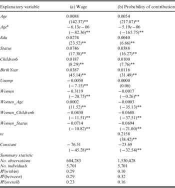
Table 1 shows the results for equations 1 and 2. For both equations (columns a and b), most variables were significant and had the expected sign. Schooling and education have a positive effect on wages; the unemployment rate has a negative sign. Being a woman has a negative effect on wages, and the year of birth has a positive effect indicating that younger cohorts have higher income levels, which is consistent with the real increase in wages experienced by the Chilean labor market. Being married and having children under 6 years of age have a positive effect on wages, but being a married woman and a woman with children less than 6 years of age have a negative effect on wages. The woman/age interaction is statistically significant and positive, implying that females' income profile is somewhat steeper than that of males. Column b shows the results for the probability of contribution. The educational level has a positive sign and the estimated parameter is significant. Unemployment is not significant in this specification. The cohort effect (BirthYear) is positive and significant. Being a woman has a negative effect on the probability of contribution. Being a married woman and/or a woman with children under 6 years of age also has a negative effect on this probability. These results are consistent with the effect of marriage and child nursing on women's employment participation and wages. The women/age interaction is statistically significant and negative, which is consistent with women's tendency to move in and out of the labor market more frequently than men.
Wage and probability of contributions – regression results

Source: Authors' calculations.
** Statistically significant at the 1% level.
For (a) the dependent variable is the log of wage.
For (b) the dependent variable is 1 when i pays contributions and 0 otherwise.
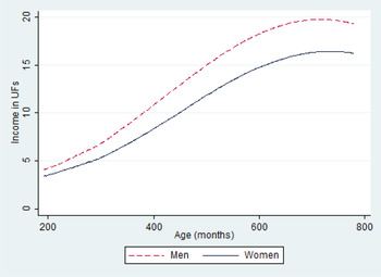
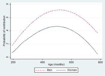
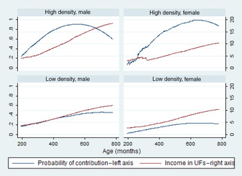
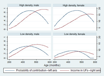
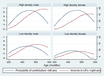
Figures 1 and 2 show the life-cycle profiles of labor incomeFootnote 6 and probability of contribution by gender. The results in Table 1 are for all individuals in the sample under analysis. In our simulation exercise, we take into account the heterogeneity observed in the data and estimate income and probability of contribution profiles by educational level and contribution density. For education, we consider three groups: (1) up to primary education, (2) secondary education and (3) tertiary education (technical degree, college and/or graduate studies). For contribution densities, we assign individuals into two different groups: low density (contribution densities between 0 and 0.50); and high density (contribution densities higher than 0.50). Therefore, we estimate 12 profiles for men and women (six profiles for labor income and six for probability of contribution for each gender). Figures (A1)–(A3) in the Appendix show these profiles.
Income profiles in UFs. Source: Authors' calculations.

Contribution profiles. Source: Authors' calculations.

3.2.2 Financial assets
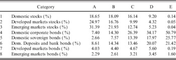
The performance of the pension funds during the accumulation phase is one of the main determinants of a member's pension upon retirement. In order to model this risk we represent the pension funds' investments through eight asset classes. Namely: domestic stocks, domestic corporate and government bonds, domestic bank bonds and deposits, international stocks in developed and emerging markets; and international bonds in developed and emerging markets. In order to map the funds' investments into these categories we focus on the pension funds' portfolio composition during December 2010. We left out earlier data since during 2008 and 2009 the funds' composition showed important changes due to a flexibilization for investments in foreign securities. The weights and indexes used to model each category are showed in Table 2. We make an important assumption by keeping the portfolios' weights fixed throughout the simulation horizon. However, currently the limits for investment in stocks and foreign securities have relaxed considerably, and there doesn't seem to be much room for regulatory changes in this direction.
Weights for pension funds mapping

Source: Authors' calculations. Categories are modeled through the following indexes: IGPA, MSCI World Index, MSCI Emerging Markets, LVACLC, LVACLG, LVACLI, Barclays Global Aggregate and JPMorgan EMBI. All the data were obtained from Bloomberg.
The results in terms of correlation between actual funds monthly returns and the mapped funds monthly returns are acceptable, ranging from 0.75 for fund E to 0.86 for funds A and B. With the set of financial indexes defined, we proceed to model the way in which they evolve over time. For this, we model returns through random walk processes with jump diffusion. Alternatives such as mean-reverting processes were discarded since, for the Chilean case, returns have exhibited a downward trend over the last decades, and therefore the long-run tendency tends to be negative for some asset classes. Since this may not be the case for international indexes, we opted for a parsimonious representation instead of using ad-hoc processes for each asset. For asset i, we assume that the monthly real return (expressed in UFs) evolves according to:
 $$dS_{i} \lpar t\rpar \sol S_{i} \lpar t\rpar \equals \mu _{i} dt \plus \sigma _{i} \varepsilon _{i\setnum{1}t} \sqrt {dt} \plus \lambda \lsqb K_{i} \plus \delta _{i} \varepsilon _{i\setnum{2}t} \rsqb .$$
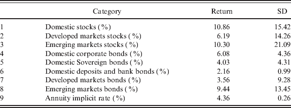
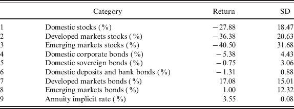
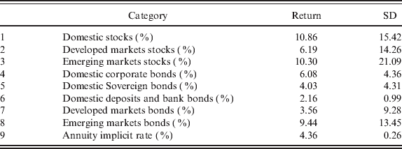
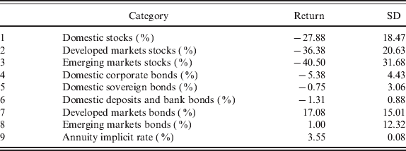
In equation (3), μi is the long-run return for asset i, whereas σi is the standard deviation. Moreover, ∊i 1t is a random shock affecting asset i's return. We assume that i's return is subject to diffuse jumps, representing financial crisis. This jump occurs with probability λ, which is set equal to 0.1059%. This implies that over his lifetime, an affiliate faces a severe crisis 3.5% of the time. Terms Ki and δi introduce deviations from the long-run return and standard deviation of asset i, respectively. The random shock ∊i 2t is assumed to be independent of ∊i 1t. Finally, we assume that assets' returns are correlated according to a 9×9 matrix Σ. The ninth asset included in this matrix is the implicit return on annuities. By doing this, we are trying to capture the extent in which adverse movements in assets' returns could be mitigated by opposite changes in annuity rates. In order to estimate Equation's (3) μi parameters we use monthly historical data from July 1996 to March 2011. The months between August 2007 and January 2009 are used to estimate the terms Ki and δi associated with returns and the Σ matrix that are used if a crisis occurs, whereas the rest of the sample is used to estimate the parameters for normal times. Tables 3 and 4 summarize the annualized returns and the standard deviation for each asset class in normal periods and for crisis.
Assets returns – normal period
Source: Authors' calculations.
Assets returns – crisis
Source: Authors' calculations.
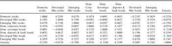
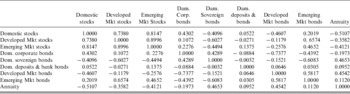
Also, Tables 5 and 6 show the Σ matrixes for the eight asset classes and the implicit annuity rates for the normal and crisis periods, respectively. As expected, the results show that during normal times domestic stocks are more correlated with emerging stock markets than with the developed ones. Also, domestic stocks show low correlations with bonds. For domestic markets bonds, there is not a big difference, in terms of correlation, with developed and emerging markets bonds. We also find that the implicit annuity rate displays a negative correlation with stock markets, especially the domestic one, while it has a relatively high correlation with domestic deposits and bank bonds. This is interesting because we would have expected annuity rates to present relatively high correlation with domestic sovereign bondsFootnote 7. As expected, during the crisis periods, domestic stocks exhibit a much larger positive correlation with foreign stock markets. We find somewhat large negative correlations between domestic stocks and domestic sovereign and developed markets bonds (−0.4096 and −0.4607, respectively), which suggest attractive hedging properties between these instruments for those periods. Domestic bond markets also show a stronger negative correlation with foreign markets bonds. Annuity rates show larger negative correlations with all stock markets. These natural hedge opportunities probably are not experienced by affiliates since they are not allowed in fund A if they are 10 years away from their legal retirement age. Finally, we do find a higher correlation between annuities and domestic sovereign bonds during the crisis periods (0.4653 versus 0.2188 for normal periods).
Assets' correlations – normal period

Source: Authors' calculations.
Assets' correlations – crisis

Source: Authors' calculations.
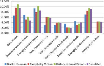
Since long-run returns are one of the key variables that determine the size of an individuals' final balance upon retirement, we explore two alternative methodologies in order to check the robustness of the parameters. Figure 3 shows the annualized real returns in Chilean pesos for the eight asset classes used in the model, as well as for annuities' rates. The returns showed correspond to those estimated following the Black–Litterman and Campbell and Viceira's methodologies (see He and Litterman, Reference He and Litterman2002 and Campbell and Viceira, Reference Campbell and Viceira2005, respectively). The figure also shows actual historic returns for the 1996–2011 periods, as well as the simulated returns. Overall, the results suggest that the asset classes' returns are reasonable.
Assets' return robustness check. Source: Author's calculations.

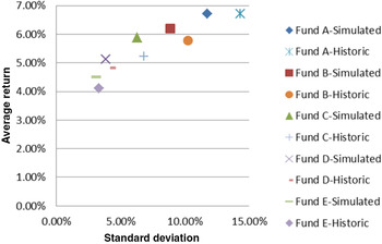
Finally, Figure 4 shows the simulated returns and standard deviations for each type of fund. The average return for fund A coincides with its historic return. This is precisely the criterion used to set the parameter λ, which governs the occurrence of crises. Although the average return for fund A is matched, the simulated standard deviation turns to be somewhat smaller. However, it is important to note that the simulated standard deviation corresponds to the mean of the standard deviations obtained after 10,000 simulations. For the rest of funds, the simulation turns out to be a little optimistic, in the sense that simulated values are higher for average returns and lower for standard deviations.Footnote 8
Pension funds' historic and simulated returns. Source: Author's calculations.

3.2.3 Human capital risk
In this subsection, we describe the methodology used in order to model human capital risk. We follow Carroll and Samwick (Reference Carroll and Samwick1997) and Cocco et al. (Reference Cocco, Gomes and Maenhout2005) and assume that prior to retirement, the log of labor income for an individual i at age t is given by:
 $${\rm log}\lpar y_{it} \rpar \equals f\hskip 1\lpar t\comma Z_{it} \rpar \plus \upsilon _{it} \plus \varepsilon _{it} \comma $$
where f(t,Zit) is a deterministic function of the individual's age and other observable characteristics, such as sex, year of birth and dummy variables to control for cohort of birth. The term ∊it corresponds to an idiosyncratic temporary disturbance, which is assumed to follow a N(0, σε) distribution, while υit is an integrated process with unitary root. This is interpreted as a permanent shock to individual i's income. This shock is equal to
 $$\upsilon _{it} \equals \upsilon _{it \minus \setnum{1}} \plus u_{it} \comma $$
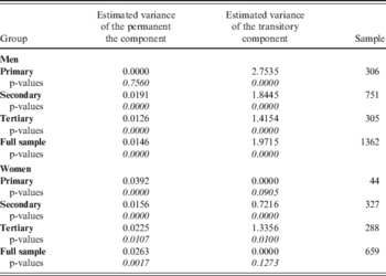
where the error term uit is assumed to follow a N(0, σu) distribution. In order to estimate equations (4) and (5), we use the same data that are employed to estimate the age-income profiles that were in Section 3.2.1. This means that we estimate a total of six equations, for males and females, with educational levels up to primary education, complete secondary education, and tertiary education. Just as in Carroll and Samwick (Reference Carroll and Samwick1997), we need to control for outliers in the regression since otherwise the results tend to be driven by a few atypical observations. Table 7 summarizes our results for the different groups. The figures obtained are not too different from those showed in Cocco et al. (Reference Cocco, Gomes and Maenhout2005) and Carroll and Samwick (Reference Carroll and Samwick1997) for the variance of the permanent component. However, our results turn out to be orders or magnitude larger for the variance of the transitory component. As Carroll and Samwick (Reference Carroll and Samwick1997) notes, the variance of the transitory component can be heavily influenced by measurement error. In our case, larger values should be expected since unlike Cocco et al. (Reference Cocco, Gomes and Maenhout2005) and Carroll and Samwick (Reference Carroll and Samwick1997) we include only labor income in our estimations, leaving out any other type of income that individuals may be receiving (e.g., transferences, welfare). Moreover, we work with monthly data, which could be subject to more measurement error as opposed to yearly observations.
The human capital risk measures are useful in our simulation methodology, since they allow us to simulate the evolution of affiliates' labor income during their working years. This is done by applying random shocks to the income profiles showed in Section 3.2.1. The volatility of the random shocks applied to labor income is obtained from Table 7. By doing this, we take into account the existing heterogeneity between representative individuals in terms of the income uncertainty that each of them faces.Footnote 9 Moreover, the human capital risk results will be used in order to interpret the replacement rates results in Section 4.
Income uncertainty by gender and education

Source: Authors' calculations.
4 Results and applications
In this section, we present the results of the simulation model. We center the discussion on the replacement rates that the representative individuals would obtain under different investment strategies. Unlike traditional pension simulators that have a deterministic nature, our model allows us to obtain information about tendency measures (average and median replacement rates) and also dispersion measures (standard deviation and confidence intervals). We also present results including social benefits as a complement of self-funded pensions and their effect on replacement rates and discuss the challenges of informing the model's results to affiliates.
4.1 Results for different investment strategies
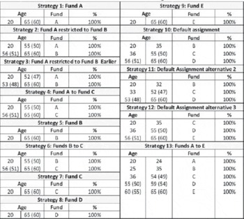
In this work, we consider a total of 12 different types of representative individuals, who vary according to gender, education and density of contribution. For each individual, we simulate the path of labor income, assets' returns and fund returns, which evolve according to the individuals' investment strategies. Taking into consideration the Chilean multi-fund framework, different investment strategies are used in the simulations. Since August 2002, both mandatory and voluntary savings have been managed under the multi-fund scheme. This consists of five types of fund (A, B, C, D and E), differentiated by the proportion of their portfolio invested in equity. Fund A is the riskiest with a 80% maximum investment limit in variable income, and fund E is the most conservative, with a 5% maximum limit in variable income. Although members are free to choose their type of fund (with some restrictions), such that it would better suite their preferences, there is also an allocation of funds by default. This default option seeks to establish an investment path that is consistent with the life cycle over the length of the member's active period. The rule for allocating members to one of the five funds consists of separating them into three age-brackets, with the younger members being placed in a fund with more equities and older members in funds with a higher proportion of fixed income. This rule is applied to both active members and pensioners. It is important to note that there are certain access restrictions.Footnote 10Table 8 shows the 13 investment alternatives that are evaluated considering combinations of the five funds, where strategy 10 is the default option in the case of Chile.
Investment strategies

Note: The ages between parentheses correspond to the relevant age for women.
We assume that individuals enter the labor force at age 20 and work until the legal retirement age (65 years for men and 60 for women).Footnote 11 For simplicity, we assume that upon retirement individuals buy a life annuity. The implicit rate for this annuity is produced within the model.Footnote 12 We calculate the replacement rates by expressing the pension received upon retirement as a fraction of the average of the income received in the last three years prior to retirement, taking into account periods without contributions, i.e., including all possible zero values for labor income in those three yearsFootnote 13. It should be noted that, even though we include contribution gaps in our estimations, we restrict the denominator of the replacement rates to be at least equal to the minimum wage under Chilean legislation (approximately USD 400 monthly dollars). Otherwise the results are distorted for those groups who make little contributions during their last working years. We argue that this approach is adequate if one wishes to evaluate the consumption smoothing properties of the pension system.Footnote 14 It is important to point that we focus on replacement rates, rather than on the amount of pensions, because the 2008 pension reform modified the Solidarity Pillar, managing to secure a minimum pension level for retirees whose income are close to the poverty line.
4.1.1 Aggregate results
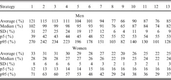
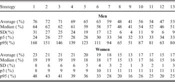
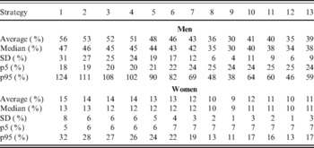
Table 9 shows the aggregate results for men and women. The replacement rates are estimated as functions of the average income in the last 3 years before retirement. The existence of contribution gaps is included to estimate average salaries. The numbers showed correspond to average replacement rates, median, standard deviation and the 5th and 95th percentiles of the distribution.Footnote 15Tables A1 and A2 in the Appendix show aggregate replacement rates as functions of the average life-time income without contribution gaps and of the last received income, respectively.Footnote 16
Replacement rates – last 3 years before retirement*

* Source: Authors' calculations. In this table, the minimum-wage restriction is binding for men and women. Strategies are: 1 – Fund A; 2 – Funds A to B; 3 – Fund A to B earlier; 4 – Fund A to C; 5 – Fund B; 6 – Fund B to C; 7 – Fund C; 8 – Fund D; 9 – Fund E; 10 – Default; 11 – Default earlier; 12 – Funds C, D and E; 13 – All funds.
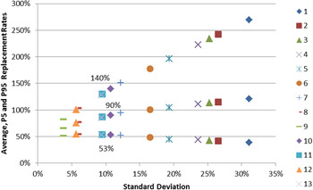
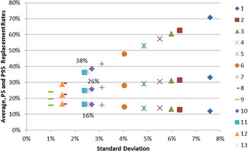
The results for the full sample of individuals suggest that affiliates face a frontier, along which they are able to select the risk–return combination that best suits their needs. For the case of the default investment strategy (Strategy 10), men have an average replacement rate of 90%, whereas this figure is considerably lower for women, reaching only 26%. This difference is mainly explained by two elements. First, women tend to have lower density of contributions, which leads to lower accumulated balances. This is true for the aggregate results, where the representative male has an average density of contributions of 56%, while females' density reaches 34.7%. Moreover, this pattern also holds for almost every group of education/density of contribution considered. Focusing on the default investment strategy, if females had the same contribution profiles as men, their average replacement rate would increase from 26% to 41%. Second, in our model, women retire 5 years earlier than men. Moreover, they have higher life expectancy. If women retired five years later, their average replacement rate would further increase up to 67%. This figure would rise to 85% if women had the same life expectancy as men. The remaining 5% gap between males and females is due to the difference among their income profiles. The default strategy turns out to be between Funds C and D in terms of average replacement rates and standard deviation. When compared to the riskiest Strategy (Strategy 1), the default allocation sacrifices around 31 percentage points in average replacement rate. However, the risk faced by affiliates is cut down almost to a third. Strategies 11 and 12 are alternative default allocations, with a more conservative profile. These strategies exhibit lower average pensions and also feature lower risk. Strategy 13 is a rich allocation in the sense that it makes full use of all five types of fund. Although similar to the current default allocation and to fund C in terms of average replacement rates and risk, it could be argued that Strategy 13 has an advantage since it keeps affiliates close to retirement in fund E, the most conservative, which is desirable if this group has little opportunity to offset negative financial performance in the years prior to retirement. Having decreasing allocations to variable income as members get older is an important feature in the design of default strategies as a risk-mitigating mechanism. In order to make up for possible losses in average returns, Strategy 13 assigns affiliates in to the riskiest fund during the first years after enrollment, when members have the longest investment horizon. Since our results suggest that a premium exists if affiliates are willing to bear more risk, the optimal degree of exposure should depend on each affiliate's preferences.Footnote 17 This implies that there are no free lunches for affiliates since any adjustment in the investment strategies in order to take less risk causes a reduction in the expected values of the replacement rates.Footnote 18Figure 5 shows the investment frontier faced by men. For instance, the default investment strategy yields an average replacement rate of 90%, while the 5th and 95th percentiles rates are 53% and 140%, respectively. For women, this numbers are 26%, 16% and 38%, respectively, as showed in Figure 6. The slopes of the average replacement rates versus standard deviation suggest that male affiliates can expect a gain (loss) of around 0.8565 percentage points in terms of average replacement rates in return for an increase (decrease) of 1 percentage point in risk, measured as standard deviation of replacement rates. For women this number is approximately 0.8572 percentage points.
Replacement rates – men – average, 5th and 95th percentiles. Source: Authors' calculations. Strategies are: 1 – Fund A; 2 – Funds A to B; 3 – Fund A to B earlier; 4 – Fund A to C; 5 – Fund B; 6 – Fund B to C; 7 – Fund C; 8 – Fund D; 9 – Fund E; 10 – Default; 11 – Default earlier; 12 – Funds C, D and E; 13 – All funds.

Replacement rates – women – average, 5th and 95th percentiles. Source: Authors' calculations. Strategies are: 1 – Fund A; 2 – Funds A to B; 3 – Fund A to B earlier; 4 – Fund A to C; 5 – Fund B; 6 – Fund B to C; 7 – Fund C; 8 – Fund D; 9 – Fund E; 10 – Default; 11 – Default earlier; 12 – Funds C, D and E; 13 – All funds.

As Figures 5 and 6 show, the implied PDF for replacement rates presents positive skewness, with extreme positive values of replacement rates having larger probability of occurrence than extremely low values. This property of the density function is relevant for affiliates, since it suggests that negative outcomes have a rather bounded probability of occurrence. Since the replacement rate is a function of many random variables, finding its analytic form is non-trivial and it is beyond our objectives for this work. However, the density functions for accumulated returns is symmetric and approximately normal, which suggests that the skewness is produced by the fact that affiliates make contributions to the pension system over their productive years. The existence of skewness in the replacement rates' PDF suggests that, in order to rank the investment strategies in terms of affiliates' expected utility, restraining to a mean-variance framework could limit the analysis. Indeed,this type of criteria ignores the fact that individuals may have preferences over other properties of the probability distribution of outcomes, such as its skewness. In order to confirm whether it is possible to rank alternatives in terms of the affiliates' expected utility, we make a stochastic dominance analysis.Footnote 19 The strongest form of stochastic dominance is that of first order. The strength of this type of dominance resides in that it allows us to rank alternatives requiring only that individuals' have positive marginal utility over wealth or replacement rates. If there is no first-order stochastic dominance, it is still possible to rank them by means of second-order stochastic dominance. Indeed, if the individual are risk averse, i.e., he has positive and decreasing marginal utility, alternative A will be preferred to B if and only if the former has second-order stochastic dominance. Finally, if it is not possible to establish the existence of second-order dominance, the criterion of third-order stochastic dominance can still be useful. In addition to the individual being risk averse, third-order dominance requires the utility function to present positive skewness (i.e., u ‴>0), i.e., faced with two alternatives with equal expected value and variance, individuals should prefer the one that displays a larger positive skewness. We attempt to rank the different investment strategies by detecting the existence of first, second or third-order stochastic dominance.Footnote 20 However, we cannot establish the existence of any dominance for men or women.Footnote 21 On the one hand, we view this result as positive, since it suggests that the current composition of pension funds does not feature dominated (and thus suboptimal) funds. On the other hand, however, this also means that a more precise definition of the affiliates' utility function must be made in order to find the optimal strategy. This is indeed an important subject, which we view as a relevant area for future research.
4.1.2 Results by education and density of contribution
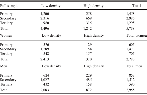
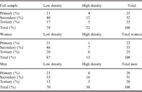
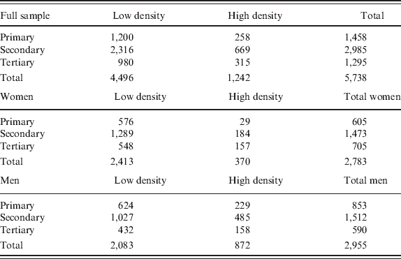
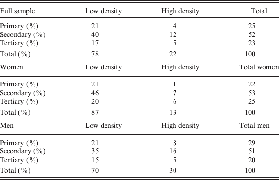
We study groups differing by level of education (primary, secondary and tertiary) and level of density of contributions (low and high). Table 10 shows the relative importance of each of these groups in our sample. Table A3 in the Appendix shows the sample size of each group.
Sample size for each education–density group
*Source: Authors' calculations.
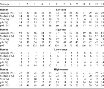
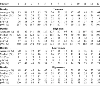
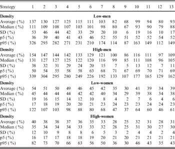
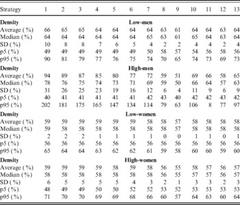
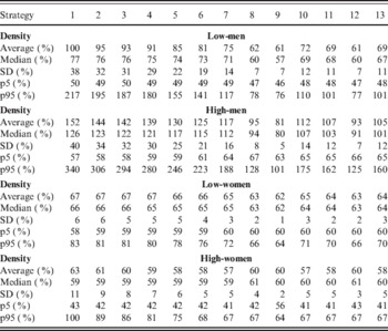
Tables 11–13 summarize the results for men and women with primary, secondary and tertiary education, respectively. It should be stressed that the large replacement rates observed for the low density with tertiary education groups are driven by the fact that both men and women in these groups show very little contributions in their last 5 years before retirement. Several conclusions can be drawn from these results. First, the slopes of the average replacement rates versus standard deviation are practically equal across genders, educational and density groups. Both male and female affiliates gain (loose) around 0.85 percentage points in terms of average replacement rates in return for an increase (decrease) of 1 percentage point in risk, measured as standard deviation of replacement rates.
Replacement rates – primary education*

* Source: Authors' calculations. In this table, the minimum wage restriction is binding for men and women with low contribution density. Strategies are: 1 – Fund A; 2 – Funds A to B; 3 – Fund A to B earlier; 4 – Fund A to C; 5 – Fund B; 6 – Fund B to C; 7 – Fund C; 8 – Fund D; 9 – Fund E; 10 – Default; 11 – Default earlier; 12 – Funds C, D and E; 13 – All funds.
Replacement rates – secondary education*

* Source: Authors' calculations. In this table, the minimum wage restriction is binding for all men and for women with low contribution density. Strategies are: 1 – Fund A; 2 – Funds A to B; 3 – Fund A to B earlier; 4 – Fund A to C; 5 – Fund B; 6 – Fund B to C; 7 – Fund C; 8 – Fund D; 9 – Fund E; 10 – Default; 11 – Default earlier; 12 – Funds C, D and E; 13 – All funds.
Replacement rates – tertiary education*

* Source: Authors' calculations. In this table, the minimum wage restriction is binding for men and women with low contribution density. Strategies are: 1 – Fund A; 2 – Funds A to B; 3 – Fund A to B earlier; 4 – Fund A to C; 5 – Fund B; 6 – Fund B to C; 7 – Fund C; 8 – Fund D; 9 – Fund E; 10 – Default; 11 – Default earlier; 12 – Funds C, D and E; 13 – All funds.
Second, it is interesting to note that replacement rates do not always increase when moving from low-density to high-density groups, keeping a constant educational level. For instance, for the default investment strategy, the average replacement rate for men with primary education goes from 31% to 69% when moving from the low-density to high-density group. Women with primary education also experiment a significant increase, going from 6% to a 21% average replacement rate. This result is similar for the secondary education group. In this case, a man with low density of contribution has an average replacement rate of 67%, whereas a man with high density has a 112% rate. For women, these figures are 15% and 37%, respectively. Finally, for the tertiary education group, a man with low density of contribution has an average replacement rate of 99%, while a man with high density has a 116% rate. For women, these figures are 41% and 32%, respectively. Although pensions are higher for individuals with higher contribution density, this does not necessarily translates to replacement rates since different income profiles have been estimated for the different groups.Footnote 22Figures A1–A3 in the Appendix show that usually the income profile of individuals with high level of contributions is monotonically increasing, which leads to pension–income ratios that can be smaller than that of individuals with a hump-shaped income profile. Since we estimate our model for different groups of representative individuals, the results could be useful in order to address the question of how much exposure to equities could be desirable for different groups. For instance, Gomez et al. (Reference Gomez, Kotlikoff and Viceira2008) suggest that the initial allocation of risky assets should be lower in the presence of increased human capital risk. In our case, we cannot give a definite answer to this issue, since as Table 7 shows, there is not a clear ordering for human capital risk across different educational levels. If one considers the distinction of men versus women the results depend on the type of variance that one wishes to prioritize. For instance, if the Regulator is more worried about permanent uncertainty (i.e., the variance of shocks with a permanent effect on income) the default allocation for women should present lower exposition to the riskier funds during early years as opposed to the allocation for men. However, if more importance is given to transitory uncertainty (i.e., the variance of shocks with a transitory effect on income) then the previous recommendation would be reversed. We also explore the existence of stochastic dominance for men and women in different education groups. Again, we cannot find evidence of the existence of dominance among investment strategies.
4.2 Role of subsidies and transfers from the Solidarity Pillar
Since 2008 the Chilean Pension System features an improved Solidarity Pillar, aimed at preventing poverty whether in old age or in the event of disability to work, to improving the pension of those affiliates with low levels of accumulated funds, and to providing a coinsurance against numerous risks. In Chile, this pillar is funded out of the nation's general taxation and includes an old-age pension, Basic Solidarity Old-Age Pension (PBS – in Spanish, Pensin Bsica Solidaria) and a complement for low old age contributory pensions, old-age Solidarity Pension Top Up (APS – in Spanish, Aporte Previsional Solidario). The system covers citizens who meet a series of requirements, such as being at least 65 years old and belong to a family group in the poorest 60% of the population. By design, the Solidarity Pillar plays two roles, it has an income redistribution feature and at the same time it mitigates market risk on pensions for the individuals transferring part of the risk to the State. This is due to the fact that the pension obtained under the Solidarity Pillar has a minimum, given by the PBS and the APS is a subsidy which is higher when savings are negatively impacted by poor investment performance of Pension Funds or negative shocks to labor income. In order to be able to evaluate the mitigating effect of the Solidarity Pillar we re-estimated the replacement rates for the different representative individuals. The Solidarity Pillar is means-tested in practice. However, our information and modelling methodology does not allow us to perform this type of tests. Therefore, here we present the results for those groups that would be more likely to benefit from the APS subsidy. Namely: men and women with primary and secondary education. Table 14 presents these results for the primary education group, while Table 15 contains the replacement rates for men and women with secondary education. These tables are comparable against the replacement rates showed in Tables 11 and 12, respectively.
Replacement rates with APS – primary education*

* Source: Authors' calculations. In this table, the minimum wage restriction is binding for men and women with low contribution density. Strategies are: 1 – Fund A; 2 – Funds A to B; 3 – Fund A to B earlier; 4 – Fund A to C; 5 – Fund B; 6 – Fund B to C; 7 – Fund C; 8 – Fund D; 9 – Fund E; 10 – Default; 11 – Default earlier; 12 – Funds C, D and E; 13 – All funds.
Replacement rates with APS – secondary education*

* Source: Authors' calculations. In this table, the minimum wage restriction is binding for all men and for women with low contribution density. Strategies are: 1 – Fund A; 2 – Funds A to B; 3 – Fund A to B earlier; 4 – Fund A to C; 5 – Fund B; 6 – Fund B to C; 7 – Fund C; 8 – Fund D; 9 – Fund E; 10 – Default; 11 – Default earlier; 12 – Funds C, D and E; 13 – All funds.
It is important to stress that, since we do not apply any means-testing requirements, our results are only illustrative. The numbers suggest that the Solidarity Pillar can have an important effect not only on the average level of replacement rates, but also on the risk faced by affiliates. Indeed, for the representative individuals in the analysis the results show that for men the volatility of the riskier investment strategies decreases, since in these cases there are scenarios with particular negative financial performance, which leads to low pensions that qualify for higher State subsidy. For the representative women the volatility is also reduced for almost every investment strategy, especially for the high density groups. Moreover, the APS subsidy has a considerable impact in the level of women's replacement rates. In summary, receiving the subsidy implies a positive effect on pensions and replacement rates and at the same time a reduction of replacement rates volatility. These results show that the Solidarity Pillar can mitigate risks for individuals in a significant level, transferring this risk to the State. This has implications for the design of the default investment strategy. In order to explore these implications, we make use of the stochastic dominance criterion. For the sake of brevity we do not report the detailed results for the comparisons among strategies. Instead, we highlight the main findings that were statistically significant. While we also summarize the dominance results for the tertiary education group, it is important to keep in mind that these representative individuals probably would not qualify to receive subsidies from the Solidarity Pillar. In the case of men with primary education, fund A dominates the rest of strategies. Moreover, riskier strategies dominate the safer ones. For the secondary education group we find safer strategies, such as Strategies 6 and 7 (Funds D and E) are always dominated by strategies with more risk. In the case of males with tertiary education, we obtain a similar finding: the safest strategy (e.g., Fund E) is dominated most of the time, whereas riskier options are never dominated. For women who have primary education, we find that safer strategies, such as Strategies 6 and 7 (Funds D and E) are always dominated by strategies with more risk. Moreover, the riskiest strategies are never dominated. In the case of women with secondary education, we only find that the safest strategy (Fund E) is dominated most of the time. Again, the riskiest strategies are never dominated. Finally, for the tertiary education group, we do not find robust dominance results. Taken as a whole, our results imply that the most appropriate investment strategies for affiliates that may qualify for the Solidarity Pillar (i.e., affiliates with both low education and low density of contributions), are those which concentrate on riskier funds. However, it is important to bear in mind that any increase in the risk of the strategies could put more pressure on Government spending in order to grant additional benefits to affiliates.
4.3 One application: informing members about pension risk
One of the permanent concerns for the Pensions Supervisor (PS) is that affiliates have all the necessary information in order to take decisions that promote their wellbeing during retirement. Since 2005 the PS has included new information in the pension statements that are received by affiliates every 4 months. This information is personalized and is sent in a yearly basis. This annex is called the Personalized Pension Projection (PPP) and it contains a forecast of the affiliates' pension under various assumptions. These statements contain information that shows the effect of expected pension from: maintaining regular contributions (for affiliates with 10 or more years to retirement) or from postponing retirement (for affiliates who have less than 10 years to reach the legal retirement age). The focus groups research undertaken so far by the SP suggests that members of the pension system appreciate the information provided in the PPP. Moreover, the available evidence (see Fajnzylber et al., Reference Fajnzylber, Plaza and Reyes2009) shows that the PPP has increased (somewhat) the probability of making voluntary contributions. Since the Chilean Pension System offers five types of funds that differ in terms of expected return and risk, if individuals focused only on the first variable, they may be tempted to select the riskier funds, which could raise the expected value of their pension funds and pension payments, but at the cost of increasing the riskiness of these variables. This is, while the expected pension payment could be increased, the probability of obtaining low pension values could also be higher. Since the current evidence shows that affiliates have a low degree of understanding of variables distinct to returns, e.g., fees and commissions. It is likely that risk-related information may not be correctly understood nor incorporated into the affiliates' decision-making process. The pension system includes safeguards against this possibility. If individuals do not explicitly choose a type of fund, they are assigned one, according to their age. Nevertheless, there is a clear need to advance in developing risk-related measures and to give this information to affiliates, in the most user-friendly manner, in order to incorporate this input and apply it to make decisions concerning their pension savings. Given the favorable experience with the PPP, the SP decided to go further and developed a pension simulator based on the methodology described in the previous sections. This simulator was launched on September 5th 2012 and it provides information on expected pensions but also on pension risk. As we have argued before, traditional measures of risk, such as standard deviation of returns, or value-at-risk, seem inadequate for long-horizon investors, which is the case for members of a pension system. The on-line application built by the PS feeds on a representative affiliates' characteristics: age, gender, level and density of contributions, age of retirement and investment strategy. Therefore, the remaining sources of risk are funds' returns and the annuities' implicit rates. One of the main challenges in this area is the low degree of understanding about risk concepts that has been detected during focus groups. While potential users show no problem in understanding the expected value concept, the idea of uncertainty is harder to grasp. First, the concept of risk tends to be associated with negative outcomes, thus ignoring the right tail of the distributions. Moreover, affiliates tended to adopt a passive posture towards risk: while affiliates are aware that they were subject to risk (e.g., low returns, losing their job, etc.), most of the time they assumed that there was nothing for them to do if they wished to reduce that risk. For instance, they are not conscious that by changing the type of funds in which their pension savings are invested, they could manage, to a certain degree, the risk associated to the returns that they could obtain. The implementation of a user-friendly pension simulator should make members aware on how to mitigate those risks and what actions they can take to increase their expected pension outcomes.
5 Conclusions
This paper stresses the importance of defining default investment strategies given the lack of financial knowledge of individuals, in particular, their low understanding of pension issues which limits their ability to take decisions. The focus is then on how to design these investment strategies and what methodology is needed to be able to properly identify the main risks faced in a defined-contribution pension system. The main goal of the design is to mitigate these risks or avoid them if possible. Many of the risks faced will persist, even where appropriate design measures are adopted or mitigation attempts made, which is why a sharing of risks among the various agents of society is also a necessary condition for the success of a pension system. We calibrate a pension risk model for the Chilean economy, including measures of life-cycle income, human capital risk, and investment and annuitization risks. This model makes the final pension its objective, which may be very different from short-term volatility. The methodology allows us to obtain forecast of future pensions for representative individuals, as well as different measures of dispersion associated to the expected outcomes, such as confidence intervals for the replacement rate to be received upon retirement. With replacement rates as our target, projections were made with interesting results that show the importance of active contributions, the impact of investment decisions and the heterogeneity in outcomes for different types of individuals. We also show how life-cycle investment strategies contribute to mitigate risks, where alternative defaults have different outcomes. Our results suggest that affiliates can expect a gain (loss) of around 0.85 percentage points in terms of average replacement rates in return for an increase (decrease) of 1 percentage point in risk, measured as standard deviation of replacement rates. An interesting result is that, as the density of contributions increases, the skewness of the density function of replacement rates increases, and the mass at the right tail of the distribution increases. This holds even though the distribution of the fund returns is symmetric. Given this, the comparison between strategies should also consider higher-order moments of the density functions associated to the replacement rates. We perform a stochastic dominance analysis to rank the different investment strategies without having to assume a specific expected utility function for affiliates. We cannot find dominated investment strategies. On the one hand, we view this result as positive, since it suggests that the current composition of pension funds does not feature dominated (and thus suboptimal) funds. On the other hand, however, this also means that a more precise definition of the affiliates' utility function must be made in order to find the optimal strategy. We view this issue as relevant for future work. Once we focus on specific education/density groups, we still find an expected gain (loss) of 0.85 percentage points in average replacement rates in exchange for a 1 percentage point increase (decrease) in standard deviation. Nevertheless, heterogeneity among individuals should be considered in a design of defaults that are specific to particular groups. These default strategies should at least consider human capital features, the existence of subsidies, other sources of financing retirement for individuals if they exist, flexibility in retirement age and available retirement products. Our stochastic dominance analysis finds no evidence of dominated strategies. Again, we believe that calibrating a life-cycle portfolio optimization model to our representative individuals seems like an interesting research area for future work. We also explore the role of the Solidarity Pillar's elements not only in providing higher pensions but also transferring risk. These features contribute to mitigate the risks that affiliates face in a defined-contribution system, but might impose a larger burden on the state. Our results imply that the most appropriate investment strategies for affiliates that may qualify for the Solidarity Pillar (e.g., affiliates with both low education and low density of contributions) are those which concentrate on riskier funds. However, it is important to bear in mind that any increase in the risk of the strategies could put more pressure on Government spending in order to grant additional benefits to affiliates. In terms of the risk faced by affiliates in a DC pension system, it is important to highlight that, even though we focused on annuities as the only pension product acquired by affiliates, in practice the existence of programmed withdrawals could also be used to mitigate the annuitization risk faced by affiliates once they reach their retirement age. Moreover, delaying retirement (when feasible) constitutes another way of hedging against adverse financial market conditions. Our model has a wide range of practical applications which go from informing affiliates about the degree of uncertainty associated to their expected pension or replacement rate to a guide in evaluating how different investment strategies affect the expected values of affiliates' pensions and their associated risk. These results are a starting point for addressing significant challenges for pension systems in terms of information to members, supervision and regulation. A proper risk measure would allow supervisors to monitor investment risk of pension funds, set limits to risk exposure, design default options, project pensions and fiscal expenses associated to subsidies for retirees, among others. For this purposes, the model could be improved by considering issues such as the behavior of fund administrators. Indeed, if administrators make significant adjustments to the portfolio of securities inside funds (e.g., reducing the exposure to equity in riskier funds during bear markets) the performance of funds will certainly change. Moreover, the behavior of affiliates could also be modeled where the resulting investment strategy would be a result of an optimization problem. These extensions could give a more accurate picture of the definite effect of different investment strategies for affiliates. In any case policy definitions with respect to target replacement rate and the level of risk tolerance at the individual and state level are required.
Appendix
Income and contribution profiles – primary education. Source: Authors' calculations.

Income and contribution profiles – secondary education. Source: Authors' calculations.

Income and contribution profiles – tertiary education. Source: Authors' calculations.

Rep. rates – average life-remuneration without gaps – no APS*

Replacement rates – last remuneration – no APS*

Sample size for educational level and contributions