





1. Introduction
Gravity current (GC) is a generic name for the buoyancy-driven flow of a fluid of one density,
 $\rho _c$
, into an ambient fluid of a different density,
 $\rho _{a}$
, mostly in horizontal direction
 $x$
(to be distinguished from the mostly vertical buoyancy-driven flows called plumes); see Ungarish (Reference Ungarish2020) and the references therein. The density difference in the (almost) hydrostatic pressure field produces a horizontal driving force in the dense fluid, called buoyancy. The buoyancy is balanced by inertial or viscous effects in the resulting motion. Here we focus attention on the so-called inertial GC, dominated by a buoyancy–inertia dynamic balance, relevant to flows at high Reynolds number. Inertial GCs have numerous applications in geophysical and environmental systems (e.g. discharges of water of different temperature/salinity into lakes and oceans, propagation of smoke in tunnels and turbidity flows; see Simpson (Reference Simpson1997) and Huppert (Reference Huppert2000) for more details). The systems of interest belong to various prototypes, such as rectangular or cylindrical geometry, Boussinesq or non-Boussinesq, driven by compositional or suspended particles effects, in inertial or rotating systems (see Ungarish (Reference Ungarish2020)). A convenient and insightful problem is the flow of a fixed volume of dense fluid released from behind a lock by the rapid opening of the front gate (dam break).
The recent works of Bingol et al. (Reference Bingol, Duran-Matute, Zhu, Meiburg and Clercx2025b ) (referred to hereafter as Betal25) and Bingol et al. (Reference Bingol, Duran-Matute, Meiburg and Clercx2025a ) focus attention on a new configuration: the GC subjected to horizontal pressure-gradient oscillations, e.g. as sketched in figure 1. The understanding of this flow is important in geophysical contexts, such as to the behaviour of salt intrusions in estuaries affected by tidal-flow pulses; the interested reader is referred to the papers of Kuijper & Van Rijn (Reference Kuijper and Van Rijn2011) and Betal25 for further details. The investigation of the flow field in this configuration also give rise to academic interest, as a significant extension to the body of knowledge on GCs.
Sketch of the system. The coordinates
 $(\tilde {x},\tilde {z})$
are fixed, while
 $(x,z)$
(origin
 $O$
) are attached to the tank which oscillates along
 $\tilde {x}$
with amplitude
 $Ax_0$
and period
 $T_{\textit{osc}}$
. At
 $t=0$
,
 $(x,z)$
and
 $(\tilde {x},\tilde {z})$
coincide, and the GC is released from a lock of length
 $x_0$
and height
 $h_0$
. The oscillations of the tank generate a pulsating background pressure field in the fluid.

Betal25 performed a direct numerical simulation (DNS) two-dimensional (2D) study of the lock-release GC subject to a periodic
 $x$
-pressure gradient pulse, using a high-resolution numerical code for a Boussinesq system (
 $\rho _{c}/\rho _{a} - 1 \ll 1$
). The influence of the stringent parameters (amplitude and period of oscillations) on the motion of the GC and structure of the flow field was carefully analysed. However, it is difficult to generalise these results because an underlying theoretical model for such flows is not available. This gap in knowledge has motivated the present work.
The importance of a theoretical model is evident. The flow depends on many parameters (those of the standard GC plus those of the oscillation) which may vary over significant ranges. The simulations of Betal25 highlight important effects, but cover a small set of parameters (full-depth lock of fixed aspect ratio, fixed Reynolds number, strictly Boussinesq, short propagation of one lock-length) and simple oscillation. It is unclear if and how the conclusions of this pioneering work can be applied in other cases. Questions concerning the influence of the height ratio of ambient to lock, the aspect ratio of the lock, non-Boussinesq effects and complex oscillations are of practical and theoretical relevance. Answering such a question using DNS is a slow and expensive procedure, because each combination of parameters requires a different run on a powerful supercomputer (as illustrated by Betal25); moreover, the interpretation of the numerical flow field is difficult without a reliable theoretical support. Laboratory experiments are also expensive and time consuming. On the other hand, an asymptotic theory based on physical governing equations is expected to cover effectively a wide range of parameters; this allows for an easy and fast analysis of trends. There is evidence that shallow-water (SW) models provide useful results for a variety of inertial lock-release GCs (e.g. with stratified and non-stratified fluids, compositional and particle driving, in horizontal or inclined channels); see Ungarish (Reference Ungarish2020) and the references therein. Here we develop and test a SW model for the present problem. We show that this model works well and yields useful insights and clear-cut predictions. We emphasise that the model does not attempt to be a substitute for the numerical simulations, just an additional efficient tool for the understanding and quick approximate estimates of the global flow.
The structure of the paper is as follow. The one-layer SW governing equations and boundary conditions are formulated in § 2. The governing dimensionless parameters, insights and predictions are presented in § 3. We show the consistency of the SW results with the simulations of Betal25. Section 4 gives some concluding remarks and suggestions for further tests (experiments and simulations).
2. Formulation
2.1. The governing equations
We use dimensional variables unless stated otherwise. The variables of the ambient fluid are denoted by the subscript
 $a$
, while those of the current are without subscript (or with subscript
 $c$
when emphasis is needed).
The system is sketched in figure 1. The GC of density
 $\rho _{c}$
is released at time
 $t=0$
from a lock of length
 $x_0$
and height
 $h_0$
into a large tank of height
 $H$
and length
 $L \gg x_0$
filled with the ambient fluid of density
 $\rho _{a}$
(
 $\lt \rho _{c}$
). We assume a 2D flow. In the
 $(x,z)$
system of coordinates attached to the tank, the velocity components are
 $u,w$
; the counterparts in the fixed system
 $(\tilde {x},\tilde {z})$
are
 $\tilde {u},\tilde {w}$
. The gravity acceleration
 $g$
acts in
 $-z$
direction.
The tank performs horizontal oscillation of amplitude
 $Ax_0$
and period
 $T_{\textit{osc}}$
which are expressed by the position of point
 $O$
(the origin of
 $(x,z)$
) as follows:
 \begin{align} \tilde {x}_O = A x_0 \sin \frac {2 \pi }{T_{\textit{osc}}} t. \end{align}
We emphasise that
 $A$
is the dimensionless amplitude of the oscillation, with reference to the lock length
 $x_0$
. (We are not concerned here with the mechanism which oscillates the tank; for definiteness, we can assume that (2.1) is imposed by a piston attached to the vertical wall
 $x=0$
.) The velocity and acceleration of the tank due to the oscillations are
 \begin{align} \tilde {u}_O = A x_0 \frac {2 \pi }{T_{\textit{osc}}} \cos \frac {2 \pi }{T_{\textit{osc}}} t , \quad \tilde {a}_O = -A x_0 \left ( \frac {2 \pi }{T_{\textit{osc}}} \right ) ^2 \sin \frac {2 \pi }{T_{\textit{osc}}} t. \end{align}
The transformation between the systems is straightforward:
 \begin{align} \tilde {x} = x+ \tilde {x}_O, \quad \tilde {u} = u+ \tilde {u}_O, \quad \tilde {w} = w. \end{align}
It is convenient to formulate the motion of the GC in the moving
 $(x,z)$
system. We assume negligible viscous effects, justified when the Reynolds number, to be defined and discussed later, is large. The momentum equations, for
 $\rho$
of the appropriate fluid, are
 \begin{align} \rho \left ( \tilde {a}_O (t) + \frac { {\rm D} u }{ {\rm D} t } \right ) = - \frac {\partial \mbox{$\mathcal P $}}{\partial x}, \\[-28pt] \nonumber \end{align}
 \begin{align} \rho \frac {{\rm D}w}{{\rm D}t} = - \frac {\partial {\mathcal P }}{\partial z} - \rho g, \\[0pt] \nonumber \end{align}
where
 $\mathcal P$
is the pressure. We define the reduced pressure
 \begin{align} p = \mbox{$\mathcal P $} + \rho _{a} g z + \rho _{a} \tilde {a}_O(t) x, \end{align}
which yields
 \begin{align} \rho \frac {{\rm D}u}{{\rm D}t} = - \frac {\partial p}{\partial x} - (\rho -\rho _{a}) \tilde {a}_O(t), \\[-28pt] \nonumber \end{align}
 \begin{align} \rho \frac {{\rm D}w}{{\rm D}t} = - \frac {\partial p }{\partial z} - (\rho - \rho _{a}) g. \\[0pt] \nonumber \end{align}
We introduce the one-layer SW approximation. The height (thickness) of the GC is
 $h(x,t)$
and the nose (denoted by subscript
 $N$
) is at
 $x_N(t)$
. We assume that the velocity of the return flow in the ambient is negligible (justified by a small
 $h/H$
), and hence for
 $z \geqslant h(x,t)$
, and for
 $x\gt x_N(t)$
, where
 $\rho = \rho _a$
, the momentum equations (2.7)–(2.8) are trivially satisfied by
 $u_a= w_a=0$
and
 $p_a =0$
.
The dense-fluid domain (the GC) is assumed to be a thin layer (
 $h/x_N \ll 1$
), and hence
 $w/u \ll 1$
, the
 $Dw/Dt$
term is negligible and (2.8) with
 $\rho =\rho _{c}$
is reduced to the hydrostatic
 $\partial p_c /\partial z = - \Delta \rho g$
where
 $\Delta \rho = \rho _{c}-\rho _{a}$
. Pressure continuity at
 $z=h(x,t)$
then yields
 $p_c = -\Delta \rho g [z-h(x,t)]$
and, hence,
 \begin{align} \frac {\partial p_c}{\partial x} (x,t) = {\Delta \rho } g \frac {\partial h}{\partial x}, \end{align}
independent of
 $z$
in the dense fluid layer. Substitution of (2.9) into (2.7), and averaging over the dense layer, gives the approximation
 \begin{align} \frac {\partial u}{\partial t} + u \frac {\partial u}{\partial x} = - \frac {\Delta \rho }{\rho _{c}} g \frac {\partial h}{\partial x} - \frac {\Delta \rho }{\rho _{c}} \tilde {a}_O(t), \end{align}
where
 $u = u(x,t)$
is the depth-averaged velocity. This momentum equation is accompanied by the usual thin-layer continuity equation
 \begin{align} \frac {\partial h}{\partial t} + \frac {\partial (h u)}{\partial x} = 0. \end{align}
The governing equations for
 $h(x,t)$
and
 $u(x,t)$
are of hyperbolic type as in the classical case of a fixed tank, and the initial conditions are also the same. The nose is therefore expected to be a jump. An inspection of the balances about the
 $x$
-thin expected jump (Ungarish Reference Ungarish2020, § 4.3) indicates that the standard Benjamin-type condition remains a good approximation (at least as long as max
 $\tilde {a}_O \ll g$
, satisfied here; see Appendix A). This gives
 \begin{align} u_N = Fr(\alpha ) \left ( \frac {\Delta \rho }{\rho _{a}} g h_N \right ) ^{1/2}, \quad \alpha =h_N/H, \end{align}
where
 $ \textit{Fr}$
is the front-jump Froude function (to be specified later).
Consider the driving effect of the full pressure,
 $\mathcal P$
. Recalling
 $p_a = 0$
, combining (2.6) with (2.9) and (2.2), and letting
 $\omega = 2 \pi / T_{\textit{osc}}$
, we obtain
 \begin{align} \frac {\partial \mbox{$\mathcal P $}}{\partial x} (x,z,t) = \left \{ \begin{array}{ll} \rho _{a} A x_0 \omega ^2 \sin \omega t + {\Delta \rho } g \frac {\partial h}{\partial x} & {\text{ in the current}} , \\[4pt] \rho _{a} A x_0 \omega ^2 \sin \omega t & {\text{ in the ambient fluid}} . \end{array} \right . \end{align}
This demonstrates that an oscillating pressure gradient, of the type considered by Betal25 ((2.4) in that paper), is present in the flow field of our model. In that paper the pressure pulse appears as
 $\cos \omega t$
, while in our paper it is
 $\sin \omega t$
, but this phase shift is insignificant for the dynamics of the flow. Betal25 did not specify the mechanism which imposes this background pulsating pressure. In our formulation, this is a necessary consequence of the boundary conditions: because the tank oscillates in the horizontal direction, the vertical side walls of the tank act like pistons on the contained fluid. (If the oscillations are defined as
 $-Ax_0 \cos \omega t$
, instead of
 $Ax_0 \sin \omega t$
, the pulse form of Betal25 is recovered. It is more convenient that both the pressure pulse
 $\sim \sin \omega t$
and the propagation begin at
 $t=0$
.) In any case, the use of the reduced pressure
 $p$
instead of
 $\mathcal P$
provides a convenient and rigorous simplification of the formulation.
We switch to dimensionless variables. Since we focus on the lock-release GC, the dominant scales that we employ are imposed by this flow (Ungarish Reference Ungarish2020). We define the reduced gravity:
 \begin{align} g' = \frac {\Delta \rho }{\rho _{c}} g; \end{align}
horizontal lengths are scaled with
 $x_0$
, vertical lengths are scaled with
 $h_0$
, velocities are scaled with
 $U$
and time with
 $T$
, where
 \begin{align} U = (g' h_0)^{1/2}, \quad T = {x_0}/{U}. \end{align}
Consider the oscillation. The amplitude of the oscillation is
 $Ax_0$
and hence the dimensionless
 $A$
is consistent with the present scaling. The next relevant dimensionless value is
 \begin{align} \tau = \frac {T_{\textit{osc}}} {T} = \frac {U T_{\textit{osc}}}{x_0}, \end{align}
which measures the period of oscillation relative to the typical time of propagation of the GC, or the distance of propagation of the GC during one cycle relative to
 $x_0$
. This can be regarded as the Keulegan–Carpenter parameter of the system. Another relevant dimensionless parameter is the ratio of the amplitude of the speed of oscillation, see (2.2), to the speed of propagation, as follows:
 \begin{align} V_O = \frac {\max \tilde {u}_O}{U} = A \frac {2 \pi }{\tau }. \end{align}
We emphasise that the dimensionless
 $A$
and
 $V_O$
are related by (2.17). It is possible to impose only one of these parameters. The acceleration
 $\tilde {a}_O$
is scaled with
 $x_0/T^2= g' h_0/x_0$
.
The formal Reynolds number of the flow is defined by
 \begin{align} Re = {U h_0}/ {\nu }, \end{align}
where
 $\nu$
is the kinematic viscosity coefficient.
We subsequently use dimensionless variables unless stated otherwise. There is no special notation for the dimensionless variables. The dimensionless equations of motion are
 \begin{align} \frac {\partial h}{\partial t} + \frac {\partial (h u) }{\partial x} = 0, \\[-28pt] \nonumber \end{align}
 \begin{align} \frac {\partial u}{\partial t} + u \frac {\partial u}{\partial x} + \frac {\partial h}{\partial x} = \left [ \frac {\Delta \rho }{\rho _{c}} V_O \frac {2 \pi }{\tau } \right ] \sin \frac {2 \pi }{\tau } t. \\[0pt] \nonumber \end{align}
The term on the right-hand side of (2.20) represents a buoyancy effect due to the background
 $x$
-acceleration (pressure oscillation) field. We call it pulse-buoyancy; this is discussed in § 2.2. We keep in mind that the terms in the momentum equation (2.20) are scaled with
 $g' h_0/x_0$
, and hence the magnitude of the right-hand side term indicates the contribution of the oscillations as compared with the standard gravity-buoyancy driving effect
 $-g' \partial h /\partial x$
.
The initial and boundary conditions are
 $u=0, h=1$
in the lock
 $0 \leqslant x \leqslant x_N = 1$
at
 $t=0$
, at the backwall
 $u(x=0, t) = 0$
, and at the front
 $x= x_N(t)$
, see (2.12),
 \begin{align} u_N = Fr(\alpha ) \left ( 1- \frac {\Delta \rho }{\rho _{c}} \right ) ^{-{1/2}} h_N ^{1/2} , \quad \alpha =h_N/H. \end{align}
The study of Huppert & Simpson (Reference Huppert and Simpson1980) provides the convenient widely used formula
 \begin{align} Fr(\alpha ) = 0.5 \alpha ^{-1/3} \quad (0.075\lt \alpha \leqslant 1), \quad Fr(\alpha ) = 1.19 \quad (\alpha \leqslant 0. 075). \end{align}
The conversion to the fixed system reads
 \begin{align} \tilde {x} = x +\left [ \frac {V_0 \tau }{2 \pi } \right ] \sin \frac {2 \pi }{\tau } t, \quad \tilde {u} = u + V_0 \cos \frac {2 \pi }{\tau } t. \end{align}
The flow field in the frame attached to the oscillating tank has been reduced to the system (2.19)–(2.22) for the variables
 $h(x,t)$
(thickness of the GC) and
 $u(x,t)$
(depth-averaged velocity of the GC). The position of the nose,
 $x_N(t)$
, is provided by the time integration of
 $u_N$
. The predicted flow depends on physical input parameters considered next.
2.2. The pulse-buoyancy effect
The input parameters of the flow are the height ratio
 $H$
of ambient to lock, the time ratio of oscillation to propagation
 $\tau$
, the speed ratio of oscillation to propagation
 $V_O$
and the density difference coefficient
 $\Delta \rho /\rho _{c}$
.
The value of
 $H$
may vary from
 $1$
(full-depth lock) to a large number (theoretically,
 $\to \infty $
) for a deep GC system.
We recall that the dimensionless oscillation amplitude
 $A = V_O \tau /(2 \pi )$
. The cases of interest in the present investigation are for
 $V_O$
close to 1, and
 $\tau$
smaller than
 $1$
, consequently
 $A$
is small (less than
 $0.1$
, say). This implies a GC flow which is affected, but not dominated, by the oscillations. The simulations of Betal25 also focus on such cases.
We consider systems with small but finite
 $\Delta \rho /\rho _{c}$
. The effect of
 $\Delta \rho /\rho _{c}$
is surprising.
1. In the strict Boussinesq approximation limit,
 $\Delta \rho /\rho _{c} \to 0$
, the pulse-buoyancy forcing term on the right-hand side of (2.20) vanishes. In this case the flow of the GC in the
 $(x,z)$
system is identical to that in a non-oscillating system. We can use the off-the-shelf SW Boussinesq results available in the literature.
We recall the main pattern of propagation (assuming that the tank is sufficiently long, see §§ 3 and 6.5.3 of Ungarish (Reference Ungarish2020), and the references therein; again, horizontal lengths are scaled with
 $x_0$
and heights with
 $h_0$
). After release, the GC enters the slumping stage in which
 $u_N$
is constant over a propagation length of about 3 (for
 $H \gt 2$
) to 10 (for
 $ H \approx 1$
), then, after some adjustment, the self-similar stage with
 $u_N \sim t^{-1/3}$
appears. When
 $x_N \approx (Re h_0/x_0) ^ {2/7}$
the GC enters into the buoyancy–viscous regime, and the SW approximation becomes invalid. Evidently, the SW results cover a long propagation in general (scaled with
 $x_0$
). Then the flow will look different in the fixed system due to the transformation (2.23). However, in the time-averaged propagation the slumping and transition lengths will be recovered, within a deviation
 $\pm A$
from the classical predictions. This difference is of little significance because, as mentioned previously,
 $A$
is small.
We obtained a general clear-cut insight: in the
 $\Delta \rho /\rho _{c} \to 0$
limit, the oscillations (pressure pulses) have no dynamic effect on the behaviour of the inertial GC; the change of behaviour observed in the fixed frame is a kinematic effect of relative translation of the fluid. In this case, dynamic effects of the oscillations can be triggered only by viscous mechanisms (not included in the SW model), and are bound to be on correspondingly small scales
 $\propto Re^{-1}$
. The simulations of Betal25 are of this type (and confirm these insights as detailed later).
2. In practical Boussinesq systems, with
 $\Delta \rho /\rho _{c}$
of a few per cent, the amplitude of the oscillatory pulse-buoyancy term in the right-hand side of (2.20) may be of the order of unity because the factor
 $2 \pi V_O/\tau$
may be 10 or larger in cases of interest. We argue that in such cases it is important to keep this forcing term in the equation.
A revisit of the Boussinesq concept supports this procedure: the inertial
 $\textrm{D} (u,w) /\textrm{D}t$
terms can be multiplied by the same
 $\rho$
(either
 $\rho _{a}$
or
 $\rho _{c}$
), but the force-field terms proportional to
 $(\rho _{c} - \rho _{a})$
are kept in the momentum equations. For the observer in the
 $(x,z)$
system, the acceleration
 $\tilde {a}_O(t)$
is a conservative body-force, like
 $g$
. Here
 $g$
pushes the fluid to the bottom. The ambient fluid of density
 $\rho _{a}$
is kept in vertical equilibrium by the
 $z$
-hydrostatic pressure field, while a particle of fluid of density
 $\rho _{c}$
is subject to the specific (buoyancy) force
 $\Delta \rho g$
towards the bottom of the tank. The acceleration
 $\tilde {a}_O$
acts similarly in the horizontal direction: when positive, it pushes towards the left wall
 $x=0$
of the tank, and when
 $\tilde {a}_O$
is negative it pushes towards the right wall. The ambient fluid is kept in horizontal equilibrium (i.e. motionless in the tank) by the
 $x$
-hydrostatic pressure field, while the dense fluid is subjected to the specific (buoyancy) force
 $\Delta \rho \tilde {a}_O$
in
 $x$
direction. The obvious difference between the body forces is that
 $\tilde {a}_O$
changes sign during the propagation of the GC, and this feature is significant when the parameter
 $\tau$
is small. The dynamics of the GC is affected by a non-trivial interaction between the body buoyancy generated by
 $g$
and
 $\tilde {a}_O$
, and the result is expressed by the dimensionless pulse buoyancy term in (2.20).
We realise that the strict Boussinesq limit (see item 1) can be justified only when
 $\Delta \rho /\rho _{c} \ll \tau /(2 \pi V_O)$
. This is a strong restriction: e.g. for the typical
 $V_O = 1, \tau = 0.3$
we obtain
 $\Delta \rho /\rho _{c} \ll 0.05$
. In the practical Boussinesq systems, it is justified to ignore the
 $\Delta \rho /\rho _{c}$
contribution in (2.21), but not in (2.20).
Two ‘silent’ important parameters are: (i) the lock aspect ratio
 $h_0/x_0$
, assumed small, and (ii) the ratio of inertial to viscous forces of the GC. The formal
 $ \textit{Re}$
is not a good estimate, because it ignores the length of the GC. For the inertial lock-release GC, the relevant parameter for the initial (slumping) phase is
 $ \textit{Re} h_0/x_0$
, assumed very large. These parameters do not enter the equations of the model, but give an indication of the validity of the inertial dominance, and determine the length where transition to the viscous regime occurs (see Ungarish (Reference Ungarish2020)).
3. Results and discussion
Typical SW results (we used a finite-difference Lax–Wendroff code) are shown in figures 2 and 3. The parameters are
 $H=2, V_O = 1, \tau = 0.294$
. The amplitude of the oscillations is
 $A = 0.0468$
, see (2.17). (The values of
 $V_O$
and
 $\tau$
were inspired by the simulations of Beta25 with
 $ \textit{Fr} = 1, KC_b = 50$
in the notation of that paper; this will be elaborated on in the following.) We performed calculations with
 $\Delta \rho /\rho _{c} = 0$
and 0.05.
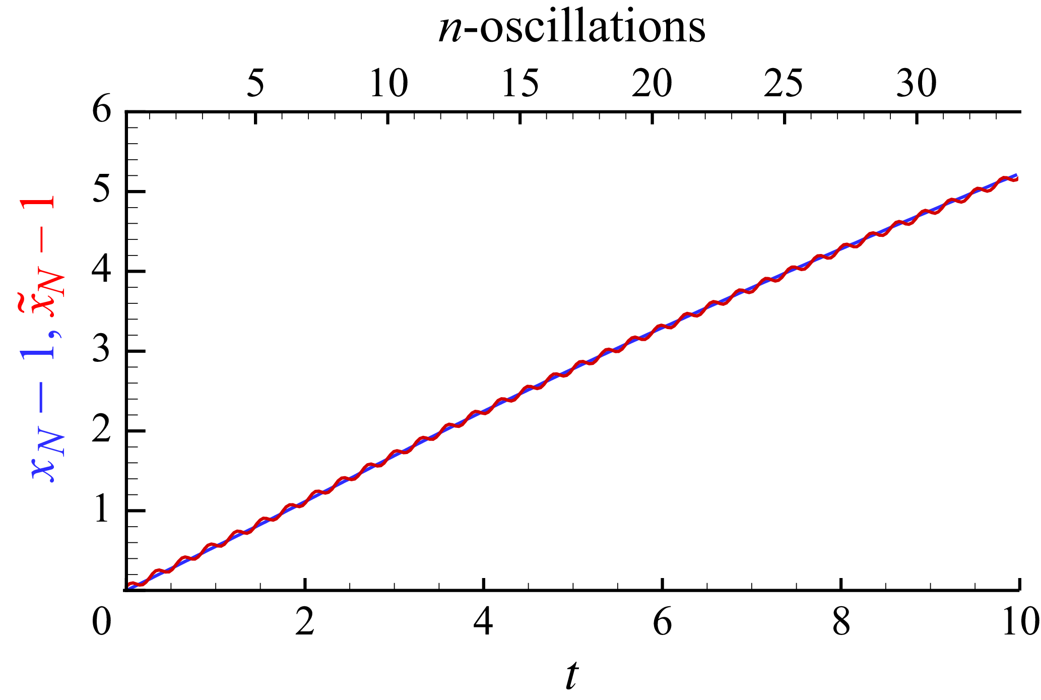
SW predictions for
 $V_O =1, \tau = 0.294, H=2$
. Plots of
 $x_N-1$
(blue line) and
 $\tilde {x}_N-1$
(red line) as functions of
 $t$
(lower axis) and number of oscillations
 $t/\tau$
(upper axis).

SW predictions for
 $V_O =1, \tau = 0.294, H=2$
. Profiles of
 $h$
and
 $u$
versus
 $x$
at
 $t = 1,2,3,4$
, for
 $\Delta \rho /\rho _{c}=0$
(blue lines) and 0.05 (red lines).

Figure 2 shows the propagation of the nose in the attached (blue line) and fixed (red line) systems. The displayed trajectory is over a significant length: the nose has propagated five lock-lengths (which implies that the average thickness has been reduced to about
 $1/6$
of the original
 $h_0$
). During this motion, the tank performed 35 oscillations. We see that, overall, the effect of the oscillations on
 $\tilde {x}_N(t)$
is quite insignificant, although
 $V_O=1$
. The reason is that the time integral of the velocity oscillations alternates as
 $\pm V_O \tau /(2 \pi ) = \pm A =\pm 0.0468$
. The change of
 $\Delta \rho /\rho _{c}$
from 0 to 0.05 has a very small effect on the propagation (the blue and red lines do not change). We tested the propagation for systems with other values of
 $H$
and
 $\tau$
, and reached the same conclusions. The
 $x_N-1 = 5$
is attained faster as
 $H$
increases, and this means fewer oscillations, but the agreement between the blue and red lines is maintained.
Figure 3 shows the profiles of
 $h$
and
 $u$
(figure 3a,b) along the GC. We see that the parameter
 $\Delta \rho /\rho _{c}$
has a significant effect on these variables. For
 $\Delta \rho /\rho _{c} \to 0$
the standard smooth profiles of the dam-break flow (blue lines) appear. For
 $\Delta \rho /\rho _{c} = 0.05$
the corresponding profiles (red lines) display wavy perturbations whose amplitude is of the order of
 $\Delta \rho /\rho _{c}$
. These oscillations are produced by the pulse-buoyancy term in the right-hand side of the momentum equation (2.20), because the coefficient
 $(\Delta \rho /\rho _{c})2 \pi V_O/\tau = 1.07$
.
The physical interpretation is as follows. The pressure pulse is tuned to the density of the ambient fluid; this fluid is accelerated like a slug between the boundaries of the container. The dense fluid reacts slightly differently to the internal pulses than the ambient fluid. Consider a small
 $t$
after the start of the motion. According to (2.20), a small increase of
 $u$
occurs in the dense fluid in the entire lock. However, the backwall at
 $x=0$
precludes motion. Consequently, a decrease of
 $h$
occurs near this wall due to continuity
 $\partial h/\partial t \approx - h \partial u/\partial x$
. This produces a positive
 $\partial h /\partial x$
(negative pressure gradient) which opposes the pulse acceleration. A similar behaviour, with more complex details, appears near the boundary
 $x_N$
. This mechanism, combined with the periodic behaviour of the forcing term, triggers an oscillation of
 $u$
and
 $h$
which is propagated into the entire body of dense fluid by the characteristics of the hyperbolic system of governing equation. (Such oscillations may enhance the interface instabilities, but such effects are expected to depend on viscous and diffusion terms which are beyond the scope of this model. This is left for future investigations.)
Figure 4 illustrates further the effect of
 $\Delta \rho /\rho _{c}$
on the profiles of
 $h$
and
 $u$
(for the same system as figure 3). We see that the increase of
 $\Delta \rho /\rho _{c}$
increases the amplitude of the wiggles, but not the number of peaks. The influence of
 $\Delta \rho /\rho _{c}$
on
 $u$
is stronger than on
 $h$
, because the velocity is directly forced by the pulse-buoyancy term. Test performed for various combinations of the parameters
 $H, \tau$
and
 $\Delta \rho /\rho _{c}$
reveal a consistent behaviour: the amplitude of the wiggles is proportional to
 $\Delta \rho /\rho _{c}$
, and the number of waves (peaks) at a fixed
 $t$
increases as
 $\tau$
decreases.
The SW profiles of
 $h$
and
 $u$
for
 $\Delta \rho /\rho _{c}=0.05$
(red lines) and
 $\Delta \rho /\rho _{c}=0.1$
(green lines), at
 $t=2$
and
 $4$
, for the system of figure 3.

Unfortunately, a comprehensive verification of the model cannot be performed at this stage because the available relevant data are scarce and cover a small parameter range. To the best of the author’s knowledge, no relevant laboratory experiments have been reported. The simulations of Betal25 are useful for testing some stringent results of the model. Both studies consider the effect of horizontal oscillations on the propagation of lock-release Boussinesq GCs. However, there are some differences between the systems which merit discussion.
The most significant discrepancy is the bottom boundary condition. The simulation apply no-slip condition at
 $z=0$
. Consider the system of figure 1. The no-slip condition is
 $u(x,z=0,t) = 0$
. (Here
 $u$
and
 $\tilde {u}$
are the physical velocities dependent on
 $x,z,t$
, not the depth-averaged values used in the SW model which do not depended on
 $z$
.) A thin viscous layer will develop under the GC for
 $x \leqslant x_N(t)$
. The ambient fluid in the domain
 $x \gt x_N(t)$
has
 $u_a=0$
, and no boundary layer appears. This is the usual situation in classical GC flows. However, the system of Betal25 is different, as sketched in figure 5: the fluid inside the oscillating tank is constrained at
 $z=0$
by no-slip on the fixed boundary,
 $\tilde {u}(x, z=0,t) =0$
. In other words, in the Betal25 flow, both the current and ambient satisfy the condition
 $u(x, z=0, t) = - \tilde {u}_O = - V_O \cos (2 \pi t/\tau )$
. Consequently, the fluid in the tank, including the ambient fluid in the upstream domain
 $x\gt x_N(t)$
, develops a viscous layer of the type predicted by Stokes’s second problem (Schlichting Reference Schlichting1979). In the system of our model, the nose of the GC encounters a homogeneous
 $u_a=0$
, while in the system of Betal25 the nose of the GC encounters a
 $z$
-profile of
 $u_a$
with a viscous layer of thickness
 $\delta \approx \sqrt {\tau x_0 /(Re h_0)}$
. For a truly large
 $ \textit{Re} h_0/x_0$
(
 $\gtrsim 10^3$
, say) the difference between the systems of figures 1 and 5 is expected to be insignificant. However, in the simulations of Betal25 (
 $ \textit{Re}=3000, h_0/x_0 = 1/170$
),
 $ \textit{Re} h_0/x_0 = 17.6$
only, and the typical
 $\delta \approx 0.13$
. In this case, the GC nose of typical
 $h_N \approx 0.50$
encounters a significant ‘obstacle’ at
 $x_N^+(t)$
. Since this obstacle-layer oscillates forth and back, the influence on the overall propagation (many cycles) is not expected to be large; however, it is expected that this layer will change the local behaviour of the nose-ambient encounter during each new cycle. (Bingol et al. (Reference Bingol, Duran-Matute, Meiburg and Clercx2025a
) is an extension of Betal25 in which an explicit Poisseuille-type viscous profile is imposed, and consequently outside the scope of the present model.)
Sketch of the system compatible with the simulations of Betal25. The vertical and top boundaries of the container oscillate as in figure 1. The fixed ground is the bottom which holds the fluids (leaks from the sides are ignored).

An inspection of the formulation of Betal25 reveals that the strict Boussinesq assumption
 $\Delta \rho /\rho _{c} \to 0$
was applied. In other words, Betal25 discards the pulse-buoyancy forcing term in the
 $x$
-momentum equations; this implies that the dynamic effect of the oscillations affects the motion in the simulations of Betal25 via the viscous terms. We also note that Betal25 solve for a full-depth lock,
 $H=1$
, which produces a significant return flow above the GC. Our one-layer model discards this return flow.
Some conversions are necessary for a comparison between Betal25 and our model. The solution of Betal25 is in the fixed
 $(\tilde {x},\tilde {z})$
system. Both studies use the same scaling for height (
 $h_0$
) and velocity (
 $U$
), and same definition of the formal
 $ \textit{Re}$
(see (2.18)). However, while we scale
 $x$
and
 $T$
with
 $x_0$
, Betal25 use the length
 $h_0$
; since
 $x_0/h_0 = 170$
in the simulations, the conversion to our scaling requires division of
 $x$
and
 $t$
of that paper by 170. In particular, the conversion of the Keulegan–Carpenter constants (
 $ \textit{KC}_b$
in Betal25) is
 $\tau = KC_b/170$
. The dimensionless speed ratio
 $V_O = \max \tilde {u}_O / {U}$
is denoted
 $ \textit{Fr}$
in Betal25 (this should not be confused with the front-jump
 $ \textit{Fr}(\alpha )$
of our model). A trivial phase shift is needed to synchronise the pulses of the simulations with the model.
We argue that the present scaling is more insightful. For example, consider the results displayed in figure 14(a) of Betal25. The plot shows a propagation of about 100 units over 400 time units; this gives the illusion of a very long process. However, comparing with the initial conditions of the simulation (figure 3 of that paper) we realise that the right-moving fluid has advanced less than one initial length (
 $x_0$
in our notation). In our scaling, that plot shows a short propagation
 $\tilde {x}_N - 1 \approx 0.6$
over
 $t \approx 2$
. The corresponding Keulegan–Carpenter
 $ \textit{KC}_b = 50$
of Betal25 gives the impression of a very long period of oscillation, but the plot shows eight periods for the propagation of one lock-length. Our
 $\tau = 0.3$
for this case is more insightful, because is indicates a short period of oscillation.
Applying the conversions and keeping in mind the special physical properties of the simulated flow, we find consistency and agreement between the results of Betal25 and the predictions of the model. In particular, support to the model is provided by the results displayed in figure 14 of Betal25. Our further mentions to figure 14 refer to this figure The simulations are for
 $\tau = 0.294$
(
 $ \textit{KC}_b = 50$
) and various
 $V_O$
in the range 0–2. The time of propagation covers eight cycles. Figure 6 shows the propagation of the GC in the fixed (laboratory) frame: SW prediction (solid lines) and Betal25 simulations (dashed lines). For the standard (no oscillations,
 $V_O = 0$
) the blue line of SW is above that of the DNS (this was expected due to the no-slip condition in the DNS code, as explained later). Consider now the results for the systems with oscillations. Both the DNS and SW plots reveal the same pattern: the red line (
 $V_O=1$
) and green line (
 $V_O = 2$
) of
 $\tilde {x}_N$
oscillate about the blue line (
 $V_O=0$
). At the end of each cycle, the position of the nose of the oscillating GC coincides with that of the unperturbed, classical GC. This conclusion is valid for all tested amplitudes
 $V_O$
; see figure 14(b). Indeed, Betal25 summarise ‘In general, the front displacement [i.e.
 $\tilde {x}_N(t)$
] after a full oscillation cycle is hardly affected by the oscillatory background flow’. This provides strong validation to the SW predictions. Moreover, the simulations show that the amplitude of the oscillations of
 $\tilde {x}_N$
satisfies the equation
 $A = V_O \tau /(2 \pi )$
(figure 14(c) and the text below). This confirms our prediction (2.17). Other plots of Beta25 (e.g. figure 4 there) also show similar agreements, but the details are more cumbersome.
In the simulations,
 $u_N$
slightly decreases with time, and the average value is
 $0.30$
. The SW predicts the constant slumping
 $u_N = 0.46$
. This discrepancy must be attributed to the viscous friction applied on the propagating GC mostly by the no-slip bottom for the non-large
 $ \textit{Re} h_0/x_0 = 17.6$
, because previously published DNS results with larger
 $ \textit{Re}$
and free-slip bottom condition (which emulate
 $ \textit{Re} \to \infty$
, e.g. Borden & Meiburg (Reference Borden and Meiburg2013)) are in good agreement with the SW value. We emphasise that the simulations reveal an interesting feature: the time-averaged viscous effect on
 $u_N$
is the same in oscillatory and non-oscillatory system. In other words, the effect of the thick oscillatory viscous layer
 $\delta \approx 0.13$
of Stokes’s second problem, cancels out on every cycle. Again, in the simulated flow field results in figure 6, the red and green lines (with
 $\delta \approx 0.13$
) collapse to the blue line (
 $\delta = 0$
) at the end of each cycle.
Comparison of DNS simulation and SW predictions for the system of Betal25 figure 14,
 $\tilde {x}-1$
as a function of
 $t$
for
 $V_O=0, 1, 2$
(blue, red, green lines). (To recover the scaling of Betal25, multiply both the distance and time by
 $x_0/h_0 = 170$
.)

We conclude that the simulations of Betal25 support the major predictions of our model. The discrepancies (such as the decrease of
 $u_N$
below the standard slumping-velocity value and the interesting lift of the nose revealed by DNS) can be attributed, with confidence, to the viscous effects which were present in the simulated flow. We argue that if similar simulations were performed with (a) a significantly larger
 $ \textit{Re} h_0/x_0$
or (b) free-slip bottom then these discrepancies would be reduced. We recall that there is a phase shift between the pulses in the simulations and the model, but this is insignificant.
4. Concluding remarks
We have developed and solved a SW model for GCs released from a lock, in a horizontally oscillating tank which produces oscillatory pressure-gradient pulses. We demonstrated that, in a system attached to the tank, the nose of the GC propagates as in the classical fixed frame of reference. However, the interface and velocity field develop additional internal waves of amplitude
 $\sim \Delta \rho /\rho _{c}$
. The predictions of our model are in good agreement with the simulations of Betal25. That study reveals various details of the flow concerning fine scales and viscous effects which are not included in our model. On the other hand, the model reveals the pulse-buoyancy effect, represented by
 $(\Delta \rho /\rho _{c})(2 \pi V_O)/ \tau$
. This effect was discarded in the simulations, but this simplification is restricted to
 $(\Delta \rho /\rho _{c}) \ll \tau /(2 \pi V_O)$
. Otherwise, the non-trivial pulse perturbations of the interface and velocity field of the GC may interact with, or even dominate, the viscous modifications This gives rise to the question what happens in realistic cases where a combination of these small effects are present. In some cases the viscous terms may suppress the buoyancy pulse, in some cases the pulse wiggles may dominate the small-scale structures about the interface. The details of these interactions is a topic for future work, using laboratory and DNS experiments. As mentioned in the introduction, the oscillatory GC is relevant to large-scale environmental applications concerning tidal flows in estuaries. On the other hand, oscillatory-flow devices are used in various industrial process (e.g. for food, semiconductors and biological fluids), but specifics applications of this study are presently unknown. In any case, we must keep in mind that the available predictions still lack experimental corroborations, which is, in our opinion, a necessary step before application. We hope that the present study will motivate and facilitate such experiments.
The model does not attempt to be a substitute for the numerical simulations, just an additional efficient tool for the understanding and quick approximate estimates of the global flow. In this context we mention that a typical simulation of Betal25 required a few days on a 400-core supercomputer, and significantly more resources will be needed to investigate systems with larger
 $ \textit{Re}$
and
 $H\gt 1$
. The predictions of the model are obtained in insignificant time on a laptop computer. The model is self-contained in the sense that it does not contain or need adjustable constants. Effects of entrainment and drag, which appear in realistic GCs, can be added to the formulation (see Ungarish Reference Ungarish2020, § 11.2), but this extension must be left for the future because the values of the entrainment and drag coefficients for the oscillating system are presently unavailable.
We have demonstrated that the pressure pulse imposed in the simulations of Betal25 and Bingol et al. (Reference Bingol, Duran-Matute, Meiburg and Clercx2025a
) can be realised by oscillating the tank. This suggests that the analysis for the flow field may be more compact in the frame of the tank than that of the laboratory. We clarified the difference between the systems of figures 1 and 5. These are important points for experimental study of the flow. Our predictions are clear cut and amenable to laboratory tests. Although simple in theory, the setup and control of GCs in oscillating tanks may pose various technical challenges (e.g. concerning the opening of the gate and leakages). Numerical simulations, e.g. with the code of Betal25, can also provide good additional tests, upon some changes of the parameters (use of
 $H\gt 1$
, larger
 $ \textit{Re}$
and free-slip conditions). The incorporation of the pulse-buoyancy effect requires some significant changes in the code.
We focused attention on a simple oscillation
 $\sim \sin 2\pi t / T_{\textit{osc}}$
. The analysis can be extended to more complex pulses using a Fourier-series decomposition.
The main restriction of the model is the one-layer simplification (the return flow in the ambient fluid is discarded). The formulation and solution of the two-layer model is a worthy topic for future work.
Acknowledgements
The author thanks Professor H. Clercx for useful discussions.
Declaration of interests
The author reports no conflict of interests.
Appendix A. The front-jump condition
In the SW formulation in the oscillating system we use the nose-jump condition (2.12) derived for non-moving containers (referred to in general as Benjamin’s formula). Here we present the justification. We use dimensional variables.
In the oscillating frame, consider the control volume attached to the jump as sketched in figure 7. The upstream and downstream velocities of the ambient fluid are
 $U$
and
 $U/(1 - \alpha )$
(due to continuity), while the velocity of the dense fluid is
 $0$
. Recall that
 $\alpha = h/H$
. The objective is to calculate (approximately) the ratio
 $U/(g' h)^{1/2}$
.
The reduced pressure
 $p$
is hydrostatic on the vertical boundaries of the control volume. In particular,
 $p=0$
on
 $ \textit{CD}$
. We use the Bernoulli equation on the streamlines
 $ \textit{CO}$
and
 $ \textit{DE}$
. (To simplify the analysis, we discard the small headloss terms which appear in the more rigorous derivation; see Ungarish & Hogg (Reference Ungarish and Hogg2018).)
For the
 $ \textit{CO}$
line we obtain
 \begin{align} p_{O-} = \frac {1}{2} \rho _{a} U^2. \end{align}
Since
 $u=0$
in the dense fluid, we obtain from (2.7)
 $\partial p_c/\partial x = - \Delta \rho \tilde {a}_O$
. Therefore, for the
 $ \textit{DEABO}$
line, we obtain
 \begin{align} p_{O+} = \frac {1}{2} \rho _{a} U^2 \left[ 1 - \frac {1}{(1-a)^2 } \right] + \Delta \rho g h + \Delta \rho \tilde {a}_O (x_B - x_O) . \end{align}
The condition
 $p_{O+} = p_{O-}$
, and some algebra, gives
 \begin{align} \frac {U^2}{\Delta \rho g h/\rho _{a} } = 2 (1-a)^2 \left [ 1 + \frac {\tilde {a}_O}{g} \frac {x_B - x_O}{h} \right ]\!. \end{align}
We argue that the contribution of last term in the brackets is very small. This term is a product of two factors, as follows. (a) The first factor
 $(x_B-x_O)/h$
is much smaller than 1, because, by definition, the nose jump is thin. (b) The second factor,
 $\tilde {a}_O/g$
, oscillates about a constant, typically non-large, value. Using (2.2) and (2.17), we find the dimensional amplitude of the acceleration term,
 $|\tilde {a}_O| = (2 \pi V_O/\tau )(h_0/x_0) g'$
. Consequently, the magnitude of the coefficient
 $\tilde {a}_O/g$
is at most
 $(\Delta \rho /\rho _{c}) (2 \pi V_O/\tau )(h_0/x_0)$
. This term is smaller than
 $1$
in all the cases of interest in our paper. (As a safety margin, we suggest restricting the analysis to cases where this term is no larger than 1; it is not clear that the model will fail for other cases, but the details require a separate investigation.) Consequently, within a small error, (A3) predicts
 \begin{align} \frac {U}{[(\rho _{c} / \rho _{a}) g' h ]^{1/2}} = \sqrt {2} (1-\alpha ), \end{align}
where
 $g' = (\Delta \rho /\rho _{c}) g$
. This result is a variant of Benjamin’s jump condition, called the circulation model
 $ \textit{Fr}(\alpha )$
result (Borden & Meiburg Reference Borden and Meiburg2013; Ungarish & Hogg Reference Ungarish and Hogg2018). The main point is that the contribution of the oscillatory background pressure vanishes in the balances that govern the jump condition in all the cases considered in this investigation, and hence off-the-shelf accepted formulae for
 $ \textit{Fr}(\alpha )$
can be used for the present system.
Sketch of the control volume attached to the front jump. Here
 $\alpha = h/H$
.


 (x~,z~)
 (x,z)
 O
 x~
 Ax0
 Tosc
 t=0
 (x,z)
 (x~,z~)
 x0
 h0
 VO=1,τ=0.294,H=2
 xN−1
 x~N−1
 t
 t/τ

 VO=1,τ=0.294,H=2
 h
 u
 x
 t=1,2,3,4
 Δρ/ρc=0

 h
 u
 Δρ/ρc=0.05
 Δρ/ρc=0.1
 t=2
 4


 x~−1
 t
 VO=0,1,2
 x0/h0=170

 α=h/H

 Open access

