1 Introduction
Turbulent wall-bounded flows with streamwise constant skin-friction coefficient
 $C_{f}$
comprise an interesting class of turbulent flows with mean-flow self-similarity. Examples for internal flows are turbulent pipe flow and open-channel flow that exhibit streamwise statistical invariance. For fully developed turbulent flow in a pipe of diameter
 $D$
with statistically uniform sand-grain-type surface roughness whose length scale
 $k_{s}$
satisfies
 $k_{s}/D\ll 1$
and where
 $k_{s}^{+}\equiv k_{s}u_{\unicode[STIX]{x1D70F}}/\unicode[STIX]{x1D708}$
is sufficiently large, the experiments of Nikuradse (Reference Nikuradse1933) showed that the average wall-friction coefficient
 $C_{f}=2\overline{\unicode[STIX]{x1D70F}}_{w}/(\unicode[STIX]{x1D70C}u_{b}^{2})$
(where
 $\overline{\unicode[STIX]{x1D70F}}_{w}$
is the average wall shear stress and
 $u_{b}$
is the bulk flow speed) becomes independent of Reynolds number
 $Re_{b}\equiv u_{b}D/\unicode[STIX]{x1D708}$
when this is sufficiently large, and depends only on
 $k_{s}/D$
. This is referred to as the ‘fully rough’ regime (see Jiménez (Reference Jiménez2004) for a discussion) where the dominant near-wall physics length scale is
 $k_{s}$
rather than the viscous scale
 $\unicode[STIX]{x1D708}/u_{\unicode[STIX]{x1D70F}}$
, where
 $u_{\unicode[STIX]{x1D70F}}^{2}=\unicode[STIX]{x1D70F}_{w}/\unicode[STIX]{x1D70C}$
is the square of the wall-friction velocity. Using a roughness correction suggested by Colebrook (Reference Colebrook1939), Moody (Reference Moody1944) developed an empirical characterization of
 $C_{f}(Re_{b},k_{s}/D)$
known as the Moody diagram that covered part of the transitionally rough regime, where both
 $Re_{b}$
and
 $k_{s}/D$
effects are present, and the fully rough regime.
The flow of a zero-pressure-gradient turbulent boundary layer (ZPGTBL) at large Reynolds number over a plate covered with sand-grain-type roughness of streamwise constant
 $k_{s}$
was considered by Prandtl & Schlichting (Reference Prandtl and Schlichting1934) and Granville (Reference Granville1958). For a plate of length
 $L$
, when
 $Re_{L}=U_{\infty }L/\unicode[STIX]{x1D708}$
becomes large, Granville developed a model showing that, if
 $k_{s}/L\ll 1$
is held constant, then the total streamwise-integrated frictional drag coefficient
 $C_{D}$
becomes independent of
 $Re_{L}$
at sufficiently large values and depends only on
 $k_{s}/L$
. Here the local skin-friction coefficient
 $C_{f}(Re_{L},k_{s}/L,x/L)$
also becomes independent of
 $Re_{L}$
but is not streamwise constant.
A class of boundary-layer flows with spatially constant skin-friction coefficient was discussed by Rotta (Reference Rotta1962), who gave quantitative arguments for the hypothesis that, for the ratio of the local outer flow speed to the skin-friction velocity to be spatially invariant, surface roughness must be present whose sand-grain-type scale
 $k_{s}$
varies linearly with streamwise distance. Specific parametrizations or calculations were not provided. Kameda et al. (Reference Kameda, Mochizuki, Osaka and Higaki2008) measured the wall skin friction for a flat-plate boundary layer over a wall in the presence of a two-dimensional
 $k$
-type roughness with length scale that varied linearly with distance
 $x$
from the leading edge. They observed that
 $U_{\infty }^{+}$
was nearly constant in
 $x$
and that the layer thickness increased linearly with
 $x$
. This idea was developed further by Talluru et al. (Reference Talluru, Djenidi, Kamruzzaman and Antonia2016), who used a self-preserving analysis based on the equations of motion to argue that the data of Kameda et al. (Reference Kameda, Mochizuki, Osaka and Higaki2008) support self-similarity of the ZPGTBL when
 $k_{s}\sim x$
.
In this paper we first develop a simple semi-empirical model for high-Reynolds-number turbulent boundary-layer flows with streamwise spatially varying, nominally sand-grain-type surface roughness in the presence of an outer flow whose velocity varies as
 $U_{\infty }=Px^{m}$
, where
 $P$
is a dimensional constant. The model makes use of the log-wake law with assumed streamwise constant parameters combined with a fully rough representation of the streamwise velocity roughness correction, and further utilizes the von Kármán boundary-layer integral equation under the assumption that all terms are constant in the streamwise direction. This shows that
 $k_{s}$
proportional to streamwise distance
 $x$
is required for closed self-similar solutions. Several cases of interest are discussed and comparisons with the results of Kameda et al. (Reference Kameda, Mochizuki, Osaka and Higaki2008) are made. The main focus is the ZPGTBL. Large-eddy simulations (LES) of this flow using a wall model with linearly varying streamwise roughness are presented. The LES utilizes the stretched-vortex subgrid-scale (SGS) model of Misra & Pullin (Reference Misra and Pullin1997) combined with the virtual-wall model (VWM) (Chung & Pullin Reference Chung and Pullin2009; Inoue & Pullin Reference Inoue and Pullin2011) for high-Reynolds-number turbulent flow that incorporates modelled SGS wall roughness (Saito, Pullin & Inoue Reference Saito, Pullin and Inoue2012). It is found that, at sufficiently large Reynolds number,
 $U_{\infty }^{+}=U_{\infty }/u_{\unicode[STIX]{x1D70F}}$
becomes independent of
 $Re_{x}$
and depends only on the dimensionless parameter
 $\unicode[STIX]{x1D6FC}$
that characterizes the roughness growth. Comparisons of LES results with model predictions are discussed.
2 Flows with linear roughness
2.1 Mean velocity profile
We consider turbulent boundary layers with power-law wall roughness
 $k_{s}=Kx^{n}$
, where
 $k_{s}$
is the local surface roughness height at the streamwise coordinate
 $x$
with origin such that both
 $k_{s}$
and all measures of the boundary-layer thickness are zero at
 $x=0$
. The length scale of streamwise roughness variation is
 $K^{1/(1-n)}$
. A Reynolds number
 $Re_{x}\equiv U_{\infty }(x)x/\unicode[STIX]{x1D708}$
is considered sufficiently large that flow is fully turbulent. It is assumed that the velocity profile within the boundary layer at any streamwise station is given by the classical log-wake relationship
 $$\begin{eqnarray}\frac{u(z)}{u_{\unicode[STIX]{x1D70F}}}=\frac{1}{\unicode[STIX]{x1D705}}\left(\log \left(\frac{(z+\unicode[STIX]{x1D700})u_{\unicode[STIX]{x1D70F}}}{\unicode[STIX]{x1D708}}\right)+\unicode[STIX]{x1D6F1}W\left(\frac{z}{\unicode[STIX]{x1D6FF}}\right)\right)-\unicode[STIX]{x0394}U^{+}\left(\frac{k_{s}u_{\unicode[STIX]{x1D70F}}}{\unicode[STIX]{x1D708}}\right)+A,\end{eqnarray}$$
where
 $\unicode[STIX]{x1D705}$
is the von Kármán constant,
 $z$
a suitably defined wall-normal distance,
 $A$
an offset constant,
 $W$
the wake function with
 $W(1)=2$
(Coles Reference Coles1956),
 $\unicode[STIX]{x1D6F1}$
the Coles wake factor and
 $\unicode[STIX]{x1D700}$
a roughness offset parameter. The latter is often used to account for an overall wall-normal shift of the logarithmic region in the presence of wall roughness (see Squire et al. (Reference Squire, Morrill-Winter, Hutchins, Schultz, Klewicki and Marusic2016) for discussion). It is expected that
 $\unicode[STIX]{x1D700}=O(k_{s})$
. In the LES to be described, first, the roughness is considered subgrid with
 $k_{s}$
smaller than the near-wall cell size, and second, we will mainly consider flows for which
 $\unicode[STIX]{x1D6FF}/k_{s}\gg 1$
. Hence this correction is presently neglected by taking
 $\unicode[STIX]{x1D700}=0$
.
In (2.1)
 $\unicode[STIX]{x0394}U(k_{s}^{+})$
is a roughness function that quantifies the effect of surface roughness on the mean velocity profile. Various forms of
 $\unicode[STIX]{x0394}U(k_{s}^{+})$
are discussed in Jiménez (Reference Jiménez2004). An implicit present assumption is that the streamwise variation of
 $\unicode[STIX]{x0394}U(k_{s}^{+})$
is sufficiently slow that the developing boundary layer can adjust to local roughness conditions. We assume a standard form for fully rough conditions,
 $$\begin{eqnarray}\unicode[STIX]{x0394}U^{+}(k_{s}^{+})=\frac{1}{\unicode[STIX]{x1D705}}\log (k_{s}^{+})+A-B,\end{eqnarray}$$
where
 $k_{s}^{+}=k_{s}u_{\unicode[STIX]{x1D70F}}/\unicode[STIX]{x1D708}$
and
 $B\approx 8.5$
is a constant. In (2.2)
 $k_{s}$
is to be interpreted as the equivalent sand-grain roughness of the surface in the sense of Nikuradse (Reference Nikuradse1933). This gives
 $$\begin{eqnarray}\frac{u(z)}{u_{\unicode[STIX]{x1D70F}}}=\left\{\begin{array}{@{}ll@{}}{\displaystyle \frac{1}{\unicode[STIX]{x1D705}}}\left(\log \left({\displaystyle \frac{z}{k_{s}}}\right)+\unicode[STIX]{x1D6F1}W\left({\displaystyle \frac{z}{\unicode[STIX]{x1D6FF}}}\right)\right)+B,\quad & z<\unicode[STIX]{x1D6FF},\\ {\displaystyle \frac{U_{\infty }}{u_{\unicode[STIX]{x1D70F}}}},\quad & z>\unicode[STIX]{x1D6FF},\end{array}\right.\end{eqnarray}$$
where the length scale
 $\unicode[STIX]{x1D6FF}$
is defined such that
 $$\begin{eqnarray}U_{\infty }^{+}\equiv \frac{U_{\infty }}{u_{\unicode[STIX]{x1D70F}}}=\frac{1}{\unicode[STIX]{x1D705}}\left(\log \left(\frac{\unicode[STIX]{x1D6FF}}{k_{s}}\right)+2\unicode[STIX]{x1D6F1}\right)+B.\end{eqnarray}$$
We utilize a simple model for the wake function (Pope Reference Pope2002):
 $$\begin{eqnarray}W\left(\frac{z}{\unicode[STIX]{x1D6FF}}\right)=2\sin ^{2}\left(\frac{\unicode[STIX]{x03C0}z}{2\unicode[STIX]{x1D6FF}}\right).\end{eqnarray}$$
The displacement thickness
 $\unicode[STIX]{x1D6FF}^{\ast }$
and the momentum thickness
 $\unicode[STIX]{x1D703}$
can now be obtained as
 $$\begin{eqnarray}\displaystyle \unicode[STIX]{x1D6FF}^{\ast } & = & \displaystyle \int _{0}^{\unicode[STIX]{x1D6FF}}\left(1-\frac{u}{U_{\infty }}\right)\text{d}z,\nonumber\\ \displaystyle & = & \displaystyle \unicode[STIX]{x1D6FF}\frac{1+\unicode[STIX]{x1D6F1}}{\unicode[STIX]{x1D705}B+2\unicode[STIX]{x1D6F1}+\log (\unicode[STIX]{x1D6FF}/k_{s})},\end{eqnarray}$$
 $$\begin{eqnarray}\displaystyle \unicode[STIX]{x1D703} & = & \displaystyle \int _{0}^{\unicode[STIX]{x1D6FF}}\frac{u}{U_{\infty }}\left(1-\frac{u}{U_{\infty }}\right)\text{d}z,\nonumber\\ \displaystyle & = & \displaystyle \unicode[STIX]{x1D6FF}\frac{\unicode[STIX]{x1D6F1}^{2}-4+2\unicode[STIX]{x1D705}B(1+\unicode[STIX]{x1D6F1})+2(1+\unicode[STIX]{x1D6F1})\log (\unicode[STIX]{x1D6FF}/k_{s})-4\unicode[STIX]{x1D6F1}Q/\unicode[STIX]{x03C0}}{2(\unicode[STIX]{x1D705}B+2\unicode[STIX]{x1D6F1}+\log (\unicode[STIX]{x1D6FF}/k_{s}))^{2}},\end{eqnarray}$$
where
 $$\begin{eqnarray}Q=\text{Si}(\unicode[STIX]{x03C0})\equiv \int _{0}^{\unicode[STIX]{x03C0}}\frac{\sin z}{z}\,\text{d}z=1.85194.\end{eqnarray}$$
In both (2.6) and (2.7) the log-wake profile is used down to
 $z=0$
. This gives integrable singularities at
 $z=0$
. Since, at large Reynolds number with
 $\unicode[STIX]{x1D6FF}\gg k_{s}$
, the roughness sublayer can be expected to make negligible contributions to the overall mass and momentum transport across the boundary layer, the error incurred is small while the analytical simplification is substantial. Also, it can be seen in (2.6) and (2.7) that both
 $\unicode[STIX]{x1D6FF}^{\ast }$
and
 $\unicode[STIX]{x1D703}$
show a nonlinear dependence on
 $\unicode[STIX]{x1D6F1}$
. The possible dependence of
 $\unicode[STIX]{x1D6F1}$
on surface roughness conditions has been discussed in the literature (Krogstad, Antonia & Browne Reference Krogstad, Antonia and Browne1992; Kameda et al.
Reference Kameda, Mochizuki, Osaka and Higaki2008). In the following model it will be required that
 $\unicode[STIX]{x1D6F1}$
be streamwise constant and so this approximation will be used subsequently.
The Rotta–Clauser parameter, sometimes used as a measure of the outer scale of the boundary layer, is defined as
 $\unicode[STIX]{x1D6E5}\equiv U_{\infty }^{+}\unicode[STIX]{x1D6FF}^{\ast }$
. Using (2.4) and (2.6) it follows that
 $$\begin{eqnarray}\frac{\unicode[STIX]{x1D6E5}}{\unicode[STIX]{x1D6FF}}=\frac{1+\unicode[STIX]{x1D6F1}}{\unicode[STIX]{x1D705}}.\end{eqnarray}$$
This is independent of the following model development.
2.2 Two-parameter model
The von Kármán integral relation can be written as
 $$\begin{eqnarray}\frac{\text{d}\unicode[STIX]{x1D703}}{\text{d}x}=\left(\frac{u_{\unicode[STIX]{x1D70F}}}{U_{\infty }}\right)^{2}-\frac{\unicode[STIX]{x1D703}}{U_{\infty }}\frac{\text{d}U_{\infty }}{\text{d}x}\left(2+\frac{\unicode[STIX]{x1D6FF}^{\ast }}{\unicode[STIX]{x1D703}}\right),\end{eqnarray}$$
where
 $U_{\infty }=U_{\infty }(x)$
and
 $u_{\unicode[STIX]{x1D70F}}=u_{\unicode[STIX]{x1D70F}}(x)$
. We now consider conditions under which all terms of (2.10) are constant. This immediately implies that
 $u_{\unicode[STIX]{x1D70F}}/U_{\infty }$
is independent of
 $x$
, and that
 $\unicode[STIX]{x1D703}\sim x$
. It then follows from (2.4) that
 $\unicode[STIX]{x1D6FF}/k_{s}$
is independent of
 $x$
and so
 $\unicode[STIX]{x1D6FF}\sim k_{s}(x)$
. If it is assumed that all of
 $\unicode[STIX]{x1D705}$
,
 $B$
and
 $\unicode[STIX]{x1D6F1}$
are independent of
 $x$
, then, since
 $\unicode[STIX]{x1D703}\sim x$
, it follows from (2.6) and (2.7) that both
 $\unicode[STIX]{x1D6FF}\sim x$
and
 $\unicode[STIX]{x1D6FF}^{\ast }\sim x$
. Since
 $\unicode[STIX]{x1D6FF}\sim k_{s}(x)$
, then the only possibility is
 $k_{s}\sim x$
in agreement with Rotta (Reference Rotta1962), Kameda et al. (Reference Kameda, Mochizuki, Osaka and Higaki2008) and Talluru et al. (Reference Talluru, Djenidi, Kamruzzaman and Antonia2016) for the zero-pressure-gradient boundary layer where
 $U_{\infty }$
is constant. Since
 $n=1$
then the flow does not contain a finite length scale associated with the streamwise variation of roughness and, at large
 $Re_{x}$
, is therefore fully self-similar with similarity variable proportional to
 $z/x$
. Hence we put
 $$\begin{eqnarray}k_{s}=\unicode[STIX]{x1D6FC}x,\end{eqnarray}$$
where
 $\unicode[STIX]{x1D6FC}$
is a dimensionless constant. For power-law outer velocity profiles
 $U_{\infty }=Px^{m}$
, where
 $P$
is a dimensional constant, it can now be seen that the second term on the right-hand side of (2.10) is constant for arbitrary
 $m$
.
Next we put
 $\unicode[STIX]{x1D6FF}=\unicode[STIX]{x1D716}\,x$
, where
 $\unicode[STIX]{x1D716}$
is to be determined. Hence
 $\unicode[STIX]{x1D6FF}/k_{s}=\unicode[STIX]{x1D716}/\unicode[STIX]{x1D6FC}$
. Substituting (2.4), (2.6) and (2.7) into (2.10) and simplifying then gives
 $$\begin{eqnarray}\displaystyle & & \displaystyle -2\unicode[STIX]{x1D705}^{2}\unicode[STIX]{x03C0}+\unicode[STIX]{x1D716}[-4-8m+2B\unicode[STIX]{x1D705}(1+3m)(1+\unicode[STIX]{x1D6F1})+\unicode[STIX]{x1D6F1}(\unicode[STIX]{x1D6F1}+m(4+6\unicode[STIX]{x1D6F1}))]\unicode[STIX]{x03C0}\nonumber\\ \displaystyle & & \displaystyle \quad -\,4\unicode[STIX]{x1D716}(1+2m)\unicode[STIX]{x1D6F1}Q+2\unicode[STIX]{x1D716}(1+3m)(1+\unicode[STIX]{x1D6F1})\unicode[STIX]{x03C0}\log (\unicode[STIX]{x1D716}/\unicode[STIX]{x1D6FC})=0.\end{eqnarray}$$
The above can be summarized as follows. We fix
 $\unicode[STIX]{x1D705}$
,
 $B$
and
 $\unicode[STIX]{x1D6F1}$
as given numerical constants (independent of
 $x$
), giving a two-parameter
 $(m,\unicode[STIX]{x1D6FC})$
model. For given
 $(m,\unicode[STIX]{x1D6FC})$
, equation (2.12) is then a transcendental equation for
 $\unicode[STIX]{x1D716}$
that can be solved numerically. We note in passing that, for given
 $\unicode[STIX]{x1D716}$
, (2.12) can in fact be solved analytically for
 $\unicode[STIX]{x1D6FC}(\unicode[STIX]{x1D716})$
, giving closed-form solutions. But we prefer to fix
 $\unicode[STIX]{x1D6FC}$
as the physical control parameter and so proceed numerically. Once
 $\unicode[STIX]{x1D716}$
is known,
 $U_{\infty }/u_{\unicode[STIX]{x1D70F}}$
follows from (2.4), while
 $\unicode[STIX]{x1D6FF}^{\ast }/x\equiv Re_{\unicode[STIX]{x1D6FF}^{\ast }}/Re_{x}$
and
 $\unicode[STIX]{x1D703}/x\equiv Re_{\unicode[STIX]{x1D703}}/Re_{x}$
can be obtained from (2.6) and (2.7), respectively. For general
 $m$
, and at finite viscosity
 $\unicode[STIX]{x1D708}$
, there exists a length scale
 $(\unicode[STIX]{x1D708}/P)^{1/(m+1)}$
and a streamwise Reynolds number
 $Re_{x}=Px^{1+m}/\unicode[STIX]{x1D708}$
. The case
 $m=0$
corresponds to the ZPGTBL with
 $P=U_{\infty }$
for which the length scale is the inverse of the unit Reynolds number
 $U_{\infty }/\unicode[STIX]{x1D708}$
. An exception is
 $m=-1$
where no length scale exists and the Reynolds number is independent of
 $x$
.
2.2.1 Asymptotic behaviour when
 $\unicode[STIX]{x1D6FC}\rightarrow 0$

If
 $\log (\unicode[STIX]{x1D716})$
is neglected compared with
 $\log (\unicode[STIX]{x1D6FC})$
in (2.12), an asymptotic form for
 $\unicode[STIX]{x1D716}$
when
 $\unicode[STIX]{x1D6FC}\rightarrow 0$
can be obtained. For illustrative purposes we display this for
 $m=0$
only as
 $$\begin{eqnarray}\unicode[STIX]{x1D716}=\frac{2\unicode[STIX]{x1D705}^{2}\unicode[STIX]{x03C0}}{(-4+\unicode[STIX]{x1D6F1}^{2}+2B\unicode[STIX]{x1D705}(1+\unicode[STIX]{x1D6F1}))\unicode[STIX]{x03C0}-4\unicode[STIX]{x1D6F1}Q-2(1+\unicode[STIX]{x1D6F1})\unicode[STIX]{x03C0}\log [\unicode[STIX]{x1D6FC}]}+\text{HOT}.\end{eqnarray}$$
When
 $\unicode[STIX]{x1D6FC}\rightarrow 0$
so that
 $|\log [\unicode[STIX]{x1D6FC}]|\gg 1$
, this becomes
 $$\begin{eqnarray}\unicode[STIX]{x1D716}\equiv \frac{\unicode[STIX]{x1D6FF}}{x}=-\frac{\unicode[STIX]{x1D705}^{2}}{(1+\unicode[STIX]{x1D6F1})\log [\unicode[STIX]{x1D6FC}]}+\text{HOT}.\end{eqnarray}$$
Substitution into (2.6) and (2.7) gives
 $$\begin{eqnarray}\frac{\unicode[STIX]{x1D6FF}^{\ast }}{x}=\left(\frac{\unicode[STIX]{x1D705}}{\log [\unicode[STIX]{x1D6FC}]}\right)^{2}+\text{HOT},\quad \frac{\unicode[STIX]{x1D703}}{x}=\left(\frac{\unicode[STIX]{x1D705}}{\log [\unicode[STIX]{x1D6FC}]}\right)^{2}+\text{HOT}.\end{eqnarray}$$
Substitution of (2.13) into (2.4) then shows that
 $$\begin{eqnarray}U_{\infty }^{+}=-\frac{1}{\unicode[STIX]{x1D705}}\log (\unicode[STIX]{x1D6FC})+O(\log (-\log (\unicode[STIX]{x1D6FC}))),\quad \unicode[STIX]{x1D6FC}\rightarrow 0,\end{eqnarray}$$
and is singular in this limit. It can be verified that (2.9) is satisfied to leading order and further that, when
 $\unicode[STIX]{x1D6FC}\rightarrow 0$
,
 $H\equiv \unicode[STIX]{x1D6FF}^{\ast }/\unicode[STIX]{x1D703}\rightarrow 1$
. The model is not asymptotic to smooth-wall flow when
 $\unicode[STIX]{x1D6FC}\rightarrow 0$
. Smooth-wall flow always requires a description of Reynolds-number effects, which are not included in the analysis.
2.3 Self-similar mean-velocity profiles
If the outer flow is given by fixing
 $m$
, the only remaining parameter is the roughness slope
 $\unicode[STIX]{x1D6FC}$
, and so all quantities are then functions of
 $\unicode[STIX]{x1D6FC}$
. For
 $\unicode[STIX]{x1D6FC}$
fixed, the mean velocity profile can now be written in a self-similar form with similarity variable
 $\unicode[STIX]{x1D702}\equiv z/(\unicode[STIX]{x1D6FC}x)$
:
 $$\begin{eqnarray}\frac{u(z)}{u_{\unicode[STIX]{x1D70F}}}=\left\{\begin{array}{@{}ll@{}}{\displaystyle \frac{1}{\unicode[STIX]{x1D705}}}\left(\log (\unicode[STIX]{x1D702})+2\unicode[STIX]{x1D6F1}\sin ^{2}\left({\displaystyle \frac{\unicode[STIX]{x03C0}\unicode[STIX]{x1D6FC}}{2\unicode[STIX]{x1D716}(\unicode[STIX]{x1D6FC})}}\unicode[STIX]{x1D702}\right)\right)+B,\quad & \unicode[STIX]{x1D702}<\unicode[STIX]{x1D716}(\unicode[STIX]{x1D6FC})/\unicode[STIX]{x1D6FC},\\ U_{\infty }^{+},\quad & \unicode[STIX]{x1D702}>\unicode[STIX]{x1D716}(\unicode[STIX]{x1D6FC})/\unicode[STIX]{x1D6FC}.\end{array}\right.\end{eqnarray}$$
Using continuity, the wall-normal velocity component is
 $$\begin{eqnarray}\frac{w(z)}{u_{\unicode[STIX]{x1D70F}}}=\left\{\begin{array}{@{}ll@{}}{\displaystyle \frac{1}{\unicode[STIX]{x1D705}}}\left[\unicode[STIX]{x1D6FC}\unicode[STIX]{x1D702}\left(1-\unicode[STIX]{x1D6F1}\cos \left({\displaystyle \frac{\unicode[STIX]{x03C0}\unicode[STIX]{x1D6FC}}{\unicode[STIX]{x1D716}(\unicode[STIX]{x1D6FC})}}\unicode[STIX]{x1D702}\right)\right)+{\displaystyle \frac{\unicode[STIX]{x1D716}(\unicode[STIX]{x1D6FC})\unicode[STIX]{x1D6F1}}{\unicode[STIX]{x03C0}}}\sin \left({\displaystyle \frac{\unicode[STIX]{x03C0}\unicode[STIX]{x1D6FC}}{\unicode[STIX]{x1D716}(\unicode[STIX]{x1D6FC})}}\unicode[STIX]{x1D702}\right)\right],\quad & \unicode[STIX]{x1D702}<\unicode[STIX]{x1D716}(\unicode[STIX]{x1D6FC})/\unicode[STIX]{x1D6FC},\\ {\displaystyle \frac{\unicode[STIX]{x1D716}(\unicode[STIX]{x1D6FC})(1+\unicode[STIX]{x1D6F1})}{\unicode[STIX]{x1D705}}},\quad & \unicode[STIX]{x1D702}>\unicode[STIX]{x1D716}(\unicode[STIX]{x1D6FC})/\unicode[STIX]{x1D6FC}.\end{array}\right.\end{eqnarray}$$
The streamline slope at
 $z=\unicode[STIX]{x1D6FF}=\unicode[STIX]{x1D716}(\unicode[STIX]{x1D6FC})x$
is
 $$\begin{eqnarray}\left(\frac{\text{d}z}{\text{d}x}\right)_{z=\unicode[STIX]{x1D6FF}}=\frac{\unicode[STIX]{x1D716}(\unicode[STIX]{x1D6FC})(1+\unicode[STIX]{x1D6F1})}{B\unicode[STIX]{x1D705}+2\unicode[STIX]{x1D6F1}+\log (\unicode[STIX]{x1D716}(\unicode[STIX]{x1D6FC})/\unicode[STIX]{x1D6FC})}.\end{eqnarray}$$
The above model can easily be formulated with
 $\unicode[STIX]{x1D6FC}$
replaced by a specified value of
 $k_{s}/\unicode[STIX]{x1D6FF}$
as the independent parameter.
3 Some special cases
Three cases of interest are now considered.
3.1 Falkner–Skan flows
For Falkner–Skan-type boundary-layer flows,
 $m=\unicode[STIX]{x1D6FD}/(2\unicode[STIX]{x03C0}-\unicode[STIX]{x1D6FD})$
, where
 $\unicode[STIX]{x1D6FD}>0$
is a wedge double angle. Here the streamwise coordinate
 $x$
has an origin at the start of the boundary layer and
 $m>0$
. The pressure gradient is favourable and it may be expected that
 $\unicode[STIX]{x1D6F1}$
is approximately constant. This case is not discussed further.
3.2 The zero-pressure-gradient turbulent boundary layer,
$m=0$

Here
 $x>0$
where
 $x=0$
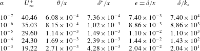
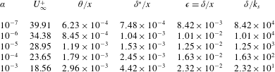
is the virtual origin of the boundary-layer growth. Tables 1 and 2 show the model parameters calculated numerically for four values of
 $\unicode[STIX]{x1D6FC}$
. First, numerical values of
 $\unicode[STIX]{x1D705}$
,
 $B$
and
 $\unicode[STIX]{x1D6F1}$
are specified with
 $m=0$
. For several values of
 $\unicode[STIX]{x1D6FC}$
, (2.12) is then solved numerically for
 $\unicode[STIX]{x1D716}=\unicode[STIX]{x1D6FF}/x$
. The quantity
 $\unicode[STIX]{x1D6FF}/k_{s}=(\unicode[STIX]{x1D6FF}/x)/(k_{s}/x)=\unicode[STIX]{x1D716}/\unicode[STIX]{x1D6FC}$
can then be calculated, which enables calculation of
 $U_{\infty }/u_{\unicode[STIX]{x1D70F}}$
using (2.4). Finally
 $\unicode[STIX]{x1D6FF}^{\ast }/x\equiv Re_{\unicode[STIX]{x1D6FF}^{\ast }}/Re_{x}$
and
 $\unicode[STIX]{x1D703}/x\equiv Re_{\unicode[STIX]{x1D703}}/Re_{x}$
are calculated using (2.6) and (2.7), respectively.
Numerical results for boundary layer with
 $m=0$
,
 $k_{s}=\unicode[STIX]{x1D6FC}x$
and
 $x>0$
. Here
 $\unicode[STIX]{x1D705}=0.384$
,
 $B=8.5$
and
 $\unicode[STIX]{x1D6F1}=0.55$
using the model of § 2.2. Values of
 $\unicode[STIX]{x1D6FC}$
specified with other quantities calculated from model as described in § 3.2.

Numerical results for boundary layer with
 $m=0$
,
 $k_{s}=\unicode[STIX]{x1D6FC}x$
and
 $x>0$
. Here
 $\unicode[STIX]{x1D705}=0.384$
,
 $B=8.5$
and
 $\unicode[STIX]{x1D6F1}=0.36$
using the model of § 2.2. Values of
 $\unicode[STIX]{x1D6FC}$
specified with other quantities calculated from model as described in § 3.2.
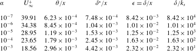
We fix
 $\unicode[STIX]{x1D705}=0.384$
and
 $B=8.5$
, which are standard values. The value of
 $\unicode[STIX]{x1D6F1}$
is somewhat uncertain. We use a standard value of
 $\unicode[STIX]{x1D6F1}=0.55$
. Then solving (2.9) for
 $\unicode[STIX]{x1D6F1}$
gives
 $\unicode[STIX]{x1D6F1}=\unicode[STIX]{x1D705}(\unicode[STIX]{x1D6E5}/\unicode[STIX]{x1D6FF})-1$
. In the LES to be described, it was found that, for the higher-resolution runs,
 $\unicode[STIX]{x1D6E5}/\unicode[STIX]{x1D6FF}_{99}=3.54$
independent of
 $\unicode[STIX]{x1D6FC}$
. If we identify
 $\unicode[STIX]{x1D6FF}_{99}(\text{LES})=\unicode[STIX]{x1D6FF}(\text{model})$
, then we calculate
 $\unicode[STIX]{x1D6F1}=0.36$
, which will be taken as an alternative value. These values are used in tables 1 and 2, respectively, which can be taken to show the effect of
 $\unicode[STIX]{x1D6F1}$
on the calculated results. Calculations were also done (not shown) using an alternative algebraic form of the wake function
 $W(z/\unicode[STIX]{x1D6FF})$
(see Jones, Marusic & Perry Reference Jones, Marusic and Perry2001) with small effect on calculated quantities for the same specified
 $\unicode[STIX]{x1D705}$
,
 $B$
and
 $\unicode[STIX]{x1D6F1}$
. In tables 1 and 2, it may be seen that, as
 $\unicode[STIX]{x1D6FC}$
increases,
 $U_{\infty }/u_{\unicode[STIX]{x1D70F}}$
decreases, meaning that
 $C_{f}$
increases with increasing roughness, in qualitative agreement with rough-wall pipe flow.
The roughness elements used by Kameda et al. (Reference Kameda, Mochizuki, Osaka and Higaki2008) for the ZPGTBL were of two-dimensional riblet-like form with rectangular cross-section. Their ratio of height
 $k$
to width
 $w$
was
 $k/w=1$
, while the element separation was
 $(b+w)/k=4$
. The local root-mean-square (r.m.s.) roughness height is
 $\unicode[STIX]{x1D70E}=\sqrt{3}/4k$
and the riblet height increased linearly as
 $\text{d}k/\text{d}x=0.00125$
. In order to compare the results of the present model with those of Kameda et al. (Reference Kameda, Mochizuki, Osaka and Higaki2008), the equivalent sand-grain roughness
 $k_{s}$
for the rectangular roughness elements must be determined. We estimate this at a single station and assume a linear dependence on the distance
 $x$
from the leading edge. From figures 7 and 9 of Kameda et al. (Reference Kameda, Mochizuki, Osaka and Higaki2008),
 $\unicode[STIX]{x0394}U^{+}\approx 13.2$
at
 $x=3.340$
m, while from their figure 4,
 $C_{f}=0.00826$
gives
 $U^{+}=15.56$
. Using
 $k_{s}^{+}\equiv k_{s}(U_{\infty }/\unicode[STIX]{x1D708})/U^{+}$
, their unit Reynolds number of
 $U_{\infty }/\unicode[STIX]{x1D708}=6.24\times 10^{5}$
m
 $^{-1}$
and substituting into (2.2) with
 $\unicode[STIX]{x1D705}=0.384$
and
 $B=8.5$
then gives
 $k_{s}\approx 0.018$
m at
 $x=3.340$
m. This gives
 $\unicode[STIX]{x1D6FC}=k_{s}/x=0.0055$
, which is 3.7 times the growth in
 $k$
given by
 $\text{d}k/\text{d}x=0.00125$
(Kameda et al.
Reference Kameda, Mochizuki, Osaka and Higaki2008) and more than 8 times the r.m.s. value of the surface roughness. Values of equivalent sand-grain roughness that are substantially larger than the physical roughness scale have been observed previously. For example, Squire et al. (Reference Squire, Morrill-Winter, Hutchins, Schultz, Klewicki and Marusic2016) report that the equivalent
 $k_{s}$
for a specific sandpaper roughness is approximately
 $13$
times the measured wall-normal r.m.s. length scale of the surface profile.
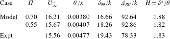
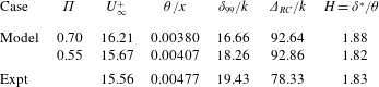
Results from the present model with
 $\unicode[STIX]{x1D6FC}=0.0055$
are shown in table 3 for two
 $\unicode[STIX]{x1D6F1}$
values,
 $\unicode[STIX]{x1D6F1}=0.70$
, the value suggested by Kameda et al. (Reference Kameda, Mochizuki, Osaka and Higaki2008), and
 $\unicode[STIX]{x1D6F1}=0.55$
. In making comparison with experiment, we have identified
 $\unicode[STIX]{x1D6FF}=\unicode[STIX]{x1D6FF}_{99}$
. The present model assumes the existence of a log regime. Jiménez (Reference Jiménez2004) remarks that
 $\unicode[STIX]{x1D6FF}/k\geqslant 40$
is needed in order to produce a finite log layer, otherwise the log layer may be suppressed by the wall-normal extent of the viscous roughness sublayer. Kameda et al. (Reference Kameda, Mochizuki, Osaka and Higaki2008) find
 $\unicode[STIX]{x1D6FF}/k\approx 19.4$
. Since we have
 $$\begin{eqnarray}k_{s}^{+}=\left(\frac{\unicode[STIX]{x1D6FF}_{99}}{k_{s}}\right)^{-1}Re_{\unicode[STIX]{x1D70F}},\end{eqnarray}$$
then large
 $k_{s}^{+}>100$
(asymptotically rough regime) coupled with large
 $\unicode[STIX]{x1D6FF}_{99}/k_{s}$
requires large
 $Re_{\unicode[STIX]{x1D70F}}$
. In Kameda et al. (Reference Kameda, Mochizuki, Osaka and Higaki2008),
 $Re_{\unicode[STIX]{x1D70F}}\sim 2200{-}4030$
, which is on the low side for this.
Comparison of present model of § 2.2 with the experiments of Kameda et al. (Reference Kameda, Mochizuki, Osaka and Higaki2008):
 $\unicode[STIX]{x1D6FC}=0.0055$
,
 $m=0$
,
 $\unicode[STIX]{x1D705}=0.384$
and
 $B=8.5$
. Here
 $\unicode[STIX]{x1D6E5}_{RC}=\unicode[STIX]{x1D6FF}^{\ast }U_{\infty }/u_{\unicode[STIX]{x1D70F}}$
is the Rotta–Clauser parameter. Values of
 $H$
for experiment obtained using an average of
 $\unicode[STIX]{x1D6FF}^{\ast }$
and
 $\unicode[STIX]{x1D703}$
tabulated in Talluru et al. (Reference Talluru, Djenidi, Kamruzzaman and Antonia2016).
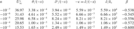
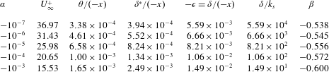
Numerical results for boundary-layer sink flow with
 $m=-1$
,
 $k_{s}=\unicode[STIX]{x1D6FC}x$
and
 $x<0$
. here
 $\unicode[STIX]{x1D705}=0.384$
,
 $B=8.5$
and
 $\unicode[STIX]{x1D6F1}=0$
using model of § 2.2. Values of
 $\unicode[STIX]{x1D6FC}$
specified with other quantities calculated from model.
3.3 Boundary-layer sink flow,
$m=-1$

Boundary-layer sink flow is given by
 $m=-1$
. Here, to a good approximation, we may take
 $\unicode[STIX]{x1D6F1}=0$
(Coles Reference Coles1957; Jones et al.
Reference Jones, Marusic and Perry2001). For this case,
 $x<0$
, with the origin of
 $x$
at the sink. Hence
 $\unicode[STIX]{x1D716}<0$
and
 $\unicode[STIX]{x1D6FC}<0$
. The calculated parameters for this flow are given in table 4. These can be seen to be qualitatively similar to those for the zero-pressure-gradient case. Pure sink flow exhibits some special features. First,
 $Re_{x}=P/\unicode[STIX]{x1D708}$
is constant; the Reynolds numbers at all streamwise stations are the same and so there exists a family of sink flows with parameter
 $P/\unicode[STIX]{x1D708}$
. In other words, with
 $P$
and
 $\unicode[STIX]{x1D708}$
fixed, large Reynolds number cannot be achieved with a sufficiently long plate. Second, the boundary layer for pure sink flow for the smooth-wall case is of equilibrium form and is self-similar (Coles Reference Coles1957). As a result, the present model applied to sink flow with linearly reducing roughness can in fact be mapped into the smooth-wall case. Calculation shows that the equivalence is
 $(u_{\unicode[STIX]{x1D70F}}/U_{\infty })\unicode[STIX]{x1D6FC}\rightarrow \unicode[STIX]{x1D708}/P$
. So for pure sink flow, both the smooth-wall flow and the sink flow with linearly decreasing roughness at large Reynolds number are self-similar.
While the Clauser parameter
 $\unicode[STIX]{x1D6FD}=(\unicode[STIX]{x1D6FF}^{\ast }/\unicode[STIX]{x1D70F}_{w})\,\text{d}p/\text{d}x$
is useful mainly for flows with adverse pressure gradients (Clauser Reference Clauser1954), it is interesting that this is exactly constant for the present class of rough-wall flows. It is straightforward to show that
 $$\begin{eqnarray}\unicode[STIX]{x1D6FD}=-m\left(\frac{U_{\infty }}{u_{\unicode[STIX]{x1D70F}}}\right)^{2}\frac{\unicode[STIX]{x1D6FF}^{\ast }}{x}\end{eqnarray}$$
and is negative for flows with favourable pressure gradients. Values for
 $m=-1$
are given in table 4. These can be seen to be small in magnitude.
4 Large-eddy simulation with wall modelling
Large-eddy simulations were performed of the ZPGTBL using wall modelling for the surface roughness, considered as subgrid. We solve the LES equations
 $$\begin{eqnarray}\displaystyle \frac{\unicode[STIX]{x2202}\widetilde{u_{i}}}{\unicode[STIX]{x2202}t}+\frac{\unicode[STIX]{x2202}\widetilde{u_{i}}\widetilde{u_{j}}}{\unicode[STIX]{x2202}x_{j}}=-\frac{\unicode[STIX]{x2202}\tilde{p}}{\unicode[STIX]{x2202}x_{i}}+\unicode[STIX]{x1D708}\frac{\unicode[STIX]{x2202}^{2}\widetilde{u_{i}}}{\unicode[STIX]{x2202}x_{j}^{2}}-\frac{\unicode[STIX]{x2202}\unicode[STIX]{x1D61B}_{ij}}{\unicode[STIX]{x2202}x_{j}},\quad \frac{\unicode[STIX]{x2202}\widetilde{u_{i}}}{\unicode[STIX]{x2202}x_{i}}=0, & & \displaystyle\end{eqnarray}$$
for the resolved velocity field
 $\widetilde{u_{i}}(x,y,z,t)$
, where
 $\unicode[STIX]{x1D61B}_{ij}\equiv \widetilde{u_{i}u_{j}}-\widetilde{u_{i}}\widetilde{u_{j}}$
is the subgrid stress tensor and where subscripted variables denote three Cartesian components in the
 $x$
(streamwise),
 $y$
(spanwise) and
 $z$
(wall-normal) directions, respectively, with corresponding velocity components
 $u$
,
 $v$
and
 $w$
. Here,
 $\widetilde{(\,)}$
refers to filtered quantities as described in Chung & Pullin (Reference Chung and Pullin2009). In the above, filtering is viewed as strictly formal.
4.1 Stretched vortex subgrid-scale model
The SGS model utilized is the stretched vortex (SV) model (Misra & Pullin Reference Misra and Pullin1997; Chung & Pullin Reference Chung and Pullin2009; Inoue & Pullin Reference Inoue and Pullin2011). This is a structure-based approach in which it is assumed that the subgrid turbulent motion in each cell is produced by modelled subgrid vortices whose orientation depends on the eigenvectors of the local resolved-scale rate-of-strain tensor. If
 $e^{v}$
is the vortex orientation, then the subgrid stress is modelled as
 $$\begin{eqnarray}\unicode[STIX]{x1D61B}_{ij}=(\unicode[STIX]{x1D6FF}_{ij}-e_{i}^{v}e_{j}^{v})K,\end{eqnarray}$$
where the subgrid energy and energy spectrum, modelled following Lundgren (Reference Lundgren1982), are
 $$\begin{eqnarray}K=\int _{k_{c}}^{\infty }E(k)\,\text{d}k,\quad E(k)={\mathcal{K}}_{0}\unicode[STIX]{x1D716}^{2/3}k^{-5/3}\exp \left(-\frac{2k^{2}\unicode[STIX]{x1D708}}{3|\overline{a}|}\right),\end{eqnarray}$$
where
 $k_{c}=\unicode[STIX]{x03C0}/\unicode[STIX]{x1D6E5}_{c}$
is the cut-off wavenumber,
 $\unicode[STIX]{x1D6E5}_{c}=(\unicode[STIX]{x1D6E5}_{x}\unicode[STIX]{x1D6E5}_{y}\unicode[STIX]{x1D6E5}_{z})^{1/3}$
and
 $a=\widetilde{\unicode[STIX]{x1D61A}}_{ij}e_{i}^{v}e_{j}^{v}$
is the projection of the resolved-scale rate of strain onto the SGS vortex direction. Integration gives
 $$\begin{eqnarray}\displaystyle K=\frac{1}{2}{\mathcal{K}}_{0}^{\prime }\unicode[STIX]{x1D6E4}\left[-\frac{1}{3},\unicode[STIX]{x1D705}_{c}^{2}\right],\quad \unicode[STIX]{x1D6E4}[s,t]=\int _{t}^{\infty }u^{s-1}\exp (-u)\,\text{d}u. & & \displaystyle\end{eqnarray}$$
Here,
 ${\mathcal{K}}_{0}^{\prime }={\mathcal{K}}_{0}\unicode[STIX]{x1D716}^{2/3}\unicode[STIX]{x1D706}_{v}^{2/3}$
is a group constant obtained by structure-function matching to the local resolved-scale flow (Chung & Pullin Reference Chung and Pullin2009; Inoue & Pullin Reference Inoue and Pullin2011),
 $\unicode[STIX]{x1D706}_{v}=(2\unicode[STIX]{x1D708}/3|\overline{a}|)^{1/2}$
and
 $\unicode[STIX]{x1D705}_{c}=k_{c}\unicode[STIX]{x1D706}_{v}$
. In the present implementation,
 $e_{i}^{v}$
is aligned with the principal extensional eigenvector of
 $\widetilde{\unicode[STIX]{x1D61A}}_{ij}$
. The SV SGS model contains assumptions but is free of adjustable model parameters save for the local cell size.
4.2 Wall model with roughness: friction velocity
$u_{\unicode[STIX]{x1D70F}}$

We utilize the virtual-wall model (VWM) (Chung & Pullin Reference Chung and Pullin2009; Inoue & Pullin Reference Inoue and Pullin2011; Cheng, Pullin & Samtaney Reference Cheng, Pullin and Samtaney2015) with inclusion of the roughness correction of Saito et al. (Reference Saito, Pullin and Inoue2012). The VWM contains two parts. In the first part, wall-normal averaging of the wall-parallel streamwise momentum equations is combined with an assumption of scaling on
 $u_{\unicode[STIX]{x1D70F}}$
and
 $\unicode[STIX]{x1D708}/u_{\unicode[STIX]{x1D70F}}$
as inner velocity and length scales for the subgrid streamwise velocity very close to the wall. For a flat wall this gives an ordinary differential equation (ODE) describing
 $u_{\unicode[STIX]{x1D70F}}(x,y,t)$
at each wall point with coefficients that are obtained dynamically from the outer LES at the first few grid points normal to the wall. The locally determined
 $u_{\unicode[STIX]{x1D70F}}$
is then used together with a log-linear-based approximation to a slip velocity at a raised or virtual plane at a specified distance
 $h_{0}$
from the wall. The scale
 $h_{0}$
is a model parameter and is subgrid in the sense that
 $h_{0}<h$
, where
 $h\equiv \unicode[STIX]{x0394}z$
is the first wall-normal grid location. Near-wall Reynolds-averaged Navier–Stokes (RANS) equations are not required and
 $u_{\unicode[STIX]{x1D70F}}(x,y,t)$
is determined dynamically. Hence
 $h_{0}^{+}\equiv h_{0}\unicode[STIX]{x1D708}/u_{\unicode[STIX]{x1D70F}}$
is determined dynamically. A two-dimensional version of the VWM is developed in Cheng et al. (Reference Cheng, Pullin and Samtaney2015) for boundary-layer separation. Since we expect attached flow in the present application, a one-wall-dimensional streamwise-centred model is used.
A description of subgrid wall roughness defined as
 $\max (k_{s})<h_{0}$
can be included in both parts of the VWM. The ODE for
 $u_{\unicode[STIX]{x1D70F}}$
and the slip and wall-normal velocities at
 $z=h_{0}$
are then (Saito et al.
Reference Saito, Pullin and Inoue2012)
 $$\begin{eqnarray}\displaystyle \frac{\text{d}u_{\unicode[STIX]{x1D70F}}}{\text{d}t}={\displaystyle \frac{\left.-{\displaystyle \frac{\unicode[STIX]{x2202}\widetilde{uu\,}}{\unicode[STIX]{x2202}x}}\right|_{h}\left.-{\displaystyle \frac{\unicode[STIX]{x2202}\widetilde{uw}}{\unicode[STIX]{x2202}z}}\right|_{h}\left.-{\displaystyle \frac{\unicode[STIX]{x2202}\widetilde{P}}{\unicode[STIX]{x2202}x}}\right|_{h}-{\displaystyle \frac{1}{h}}\widetilde{uv}\mid _{h}\left.+{\displaystyle \frac{\unicode[STIX]{x1D708}}{h}}{\displaystyle \frac{\unicode[STIX]{x2202}\widetilde{u}}{\unicode[STIX]{x2202}y}}\right|_{h}-{\displaystyle \frac{1}{h}}u_{\unicode[STIX]{x1D70F}}^{2}}{{\displaystyle \frac{\widetilde{u}\mid _{h}}{u_{\unicode[STIX]{x1D70F}}}}-k_{s}^{+}{\displaystyle \frac{\unicode[STIX]{x2202}\unicode[STIX]{x0394}U^{+}}{\unicode[STIX]{x2202}k_{s}^{+}}}}}, & & \displaystyle\end{eqnarray}$$
while the streamwise and wall-normal slip flow velocities at the raised virtual wall
 $z=h_{0}$
are, respectively,
 $$\begin{eqnarray}\displaystyle & \displaystyle \widetilde{u}\mid _{h_{0}}=u_{\unicode[STIX]{x1D70F}}\left({\displaystyle \frac{1}{{\mathcal{K}}_{1}}}\log (h_{0}^{+})+B-\unicode[STIX]{x0394}U^{+}(k_{s}^{+})\right), & \displaystyle\end{eqnarray}$$
 $$\begin{eqnarray}\displaystyle & \displaystyle \widetilde{w}\mid _{h_{0}}=-h_{0}{\displaystyle \frac{\unicode[STIX]{x2202}u_{\unicode[STIX]{x1D70F}}}{\unicode[STIX]{x2202}x}}\left({\displaystyle \frac{\tilde{u} \mid _{h_{0}}}{u_{\unicode[STIX]{x1D70F}}}}-k_{s}^{+}{\displaystyle \frac{\unicode[STIX]{x2202}\unicode[STIX]{x0394}U^{+}}{\unicode[STIX]{x2202}k_{s}^{+}}}\right). & \displaystyle\end{eqnarray}$$
In the above,
 ${\mathcal{K}}_{1}$
is an instantaneous local von Kármán constant that is calculated dynamically (Chung & Pullin Reference Chung and Pullin2009). The function
 $\unicode[STIX]{x0394}U^{+}(k_{s}^{+})$
is a model-specified roughness correction that may vary across the wall. We use (2.2) with
 $k_{s}(x)$
given by (2.11) with
 $\unicode[STIX]{x1D6FC}$
specified. The present wall model, including the roughness correction, is entirely local so that on the wall
 $u_{\unicode[STIX]{x1D70F}}=u_{\unicode[STIX]{x1D70F}}(x,y,t)$
. As a result of this space and time variation, both
 $k_{s}^{+}$
and thus
 $\unicode[STIX]{x0394}U^{+}(k_{s}^{+})$
also vary spatially and temporally on the wall. Subsequently, when referring to LES results, we use the notation
 $\overline{u}_{\unicode[STIX]{x1D70F}}$
to refer to either time or spatially averaged values but, for simplicity, redefine
 $u^{+}=u/\overline{u}_{\unicode[STIX]{x1D70F}}$
and
 $U^{+}=U_{\infty }/\overline{u}_{\unicode[STIX]{x1D70F}}$
.
4.3 Numerical method
The numerical method for LES of boundary-layer flow is described in detail in Inoue & Pullin (Reference Inoue and Pullin2011) and Cheng et al. (Reference Cheng, Pullin and Samtaney2015). Equations (4.1) and (4.5) are integrated in time using the three-stage low-storage Runge–Kutta method (Spalart, Moser & Rogers Reference Spalart, Moser and Rogers1991). At each stage, the fractional-step method (Perot Reference Perot1993) is utilized. With implicit treatment of the viscous term in the wall-normal direction, this gives a modified Helmholtz equation for the velocity update together with a Poisson equation for pressure followed by a velocity correction step. A staggered grid is used in the streamwise–wall-normal (
 $x{-}z$
) plane where the (
 $u,w$
) velocity components are stored at the centres of (
 $x,z$
) cell faces with cell-centred storage in the
 $y$
direction. For spatial discretization, a fourth-order-accurate finite-difference scheme is utilized in the
 $x$
and
 $z$
directions while a pseudo-spectral representation is employed in the
 $y$
direction. Energy conservation and dealiasing are improved by using the skew-symmetric form of convective terms. For pressure the relevant Poisson equation reduces to a sequence of one-dimensional equations in the
 $z$
direction by combining a spectral representation in
 $y$
with a fast-cosine transform in
 $x$
. The overall numerical method has been tested using direct numerical simulation (Inoue & Pullin Reference Inoue and Pullin2011) of the turbulent boundary layer at low
 $Re_{\unicode[STIX]{x1D703}}$
.
The flow is spanwise (
 $y$
) periodic, has a prescribed velocity
 $w_{top}$
at the upper boundary of the computational domain, and a convective boundary condition at the streamwise exit plane, as follows:
 $$\begin{eqnarray}\displaystyle w_{top}=U_{\infty }\frac{\text{d}\unicode[STIX]{x1D6FF}^{\ast }}{\text{d}x},\quad \frac{\unicode[STIX]{x2202}\boldsymbol{u}}{\unicode[STIX]{x2202}t}=U_{c}(z)\frac{\unicode[STIX]{x2202}\boldsymbol{u}}{\unicode[STIX]{x2202}x}, & & \displaystyle\end{eqnarray}$$
where
 $U_{c}(z)$
is the mean streamwise exit velocity. The value
 $\text{d}\unicode[STIX]{x1D6FF}^{\ast }/\text{d}x$
is represented by a single streamwise average (Inoue & Pullin Reference Inoue and Pullin2011). A turbulent initial condition is used, and turbulent flow is sustained through an inflow condition generated by a recycling method described in the following section.
4.4 Recycling
For generating the inflow, we refer to the recycling method by Lund, Wu & Squires (Reference Lund, Wu and Squires1998), in which the components of inflow velocity, including mean and fluctuation parts, are mapped from the flow field at an internal plane. This mapping idea originates from the scaling-similarity property of boundary-layer flow. Similar to the classical scaling, the recycling method recognizes an inner region and an outer region. In the original recycling method for ZPGTBL flow, velocity components in the inner region (inn) are mapped using the law of the wall, which means the scaled coordinate is
 $z^{+}=z/l^{+}$
with
 $l^{+}=\unicode[STIX]{x1D708}/u_{\unicode[STIX]{x1D70F}}$
. In the outer region (out), velocity components are recycled using the defect law, where the scaled coordinate is
 $\unicode[STIX]{x1D702}=z/\unicode[STIX]{x1D6FF}$
with
 $\unicode[STIX]{x1D6FF}$
some measure of the boundary-layer thickness. For the entire recycling process, velocity components are scaled using
 $u_{\unicode[STIX]{x1D70F}}$
.
The formula used for the recycling method can thus be summarized as follows:
 $$\begin{eqnarray}\displaystyle \unicode[STIX]{x1D719}_{in}^{inn}=\unicode[STIX]{x1D719}_{re}^{inn},\quad \unicode[STIX]{x1D719}_{in}^{out}=\unicode[STIX]{x1D719}_{re}^{out}, & & \displaystyle\end{eqnarray}$$
where
 $\unicode[STIX]{x1D719}$
denotes the velocity component, either the mean streamwise velocity
 $u(z)$
, the mean wall-normal velocity
 $w(z)$
, or three fluctuation components
 $u^{\prime }(y,z)$
,
 $v^{\prime }(y,z)$
and
 $w^{\prime }(y,z)$
. The subscripts ‘
 $in$
’ and ‘
 $re$
’ for the inlet plane and recycling plane indicate the position where velocity components are evaluated. The superscripts ‘
 $inn$
’ and ‘
 $out$
’ denote different scaled coordinates, as discussed above.
In generating the inflow velocity, a weighted function is defined to combine the velocity components in the inner region and outer region. This procedure closely follows the original recycling method, and its detailed description is not repeated here. In the implementation of the recycling procedure, the mirroring method by Jewkes, Chung & Carpenter (Reference Jewkes, Chung and Carpenter2011), which serves to almost remove the spatially quasi-periodic effect, is used.
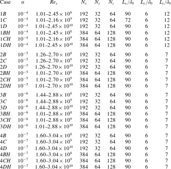
Summary of zero-pressure-gradient LES with linear roughness. Numbers represent the particular case of
 $\unicode[STIX]{x1D6FC}$
. Letters represent different inflow
 $Re_{x}$
order of magnitude:
 $B$
,
 $10^{8}$
;
 $C$
,
 $10^{9}$
;
 $D$
,
 $10^{10}$
;
 $H$
represents a high-resolution simulation.

4.5 Large-eddy simulation performed
The LES were performed on a rectangular domain. Parameters for the LES discussed are summarized in table 5. In what follows we refer to two streamwise coordinates
 $x$
and
 $x^{\prime }$
related by
 $x^{\prime }=x-x_{0}$
. The coordinate
 $x^{\prime }$
has origin
 $x^{\prime }=0$
at the domain inlet while the origin of
 $x$
is the nominal flat-plate leading edge. Each individual LES was performed on a rectangular domain with inlet at
 $x=x_{0},~x^{\prime }=0$
where the determination of
 $x_{0}$
is to be discussed. At the domain inlet, in computational coordinates,
 $\unicode[STIX]{x1D6FF}_{99}$
, the 99 % boundary-layer thickness is set to unit length. With
 $\unicode[STIX]{x1D708}$
specified and
 $U_{\infty }=1$
, this fixes the nominal inlet Reynolds number
 $Re_{\unicode[STIX]{x1D6FF}_{99}}=\unicode[STIX]{x1D6FF}_{99}U_{\infty }/\unicode[STIX]{x1D708}$
. For each LES the fixed parameters are then
 $\unicode[STIX]{x1D6FF}_{99}$
,
 $U_{\infty }$
,
 $\unicode[STIX]{x1D708}$
and the streamwise roughness growth rate
 $\unicode[STIX]{x1D6FC}$
. We note that
 $k_{s}=\unicode[STIX]{x1D6FC}x$
and denote by
 $k_{s,0}=\unicode[STIX]{x1D6FC}x_{0}$
the roughness height at the domain inlet
 $x=x_{0}$
.
For given
 $\unicode[STIX]{x1D6FC}$
, denote the value of
 $\unicode[STIX]{x1D6FF}/k_{s}$
given by the empirical model (see table 1) by
 $(\unicode[STIX]{x1D6FF}/k_{s})_{model}$
. Then identifying
 $\unicode[STIX]{x1D6FF}_{99}=\unicode[STIX]{x1D6FF}$
, an initial estimate of
 $x_{0}$
is
 $$\begin{eqnarray}x_{0}=\frac{1}{\unicode[STIX]{x1D6FC}}\left(\frac{\unicode[STIX]{x1D6FF}}{k_{s}}\right)_{model}^{-1}.\end{eqnarray}$$
With
 $x_{0}$
known, LES is then performed with fixed parameters and with
 $k_{s}$
calculated as
 $k_{s}(x)=\unicode[STIX]{x1D6FC}x=\unicode[STIX]{x1D6FC}(x^{\prime }+x_{0})$
. It was found that, following the usual transient to statistically steady flow,
 $\unicode[STIX]{x1D703}(x)$
obtained from the LES showed a strong linear correlation with
 $x^{\prime }$
downstream of the recycling region, but that its virtual origin was near to but not at the present
 $x_{0}$
. An updated
 $x_{0}$
was then calculated using linear extrapolation of
 $\unicode[STIX]{x1D703}$
in
 $x^{\prime }$
to determine a virtual leading-edge origin
 $x^{\prime }=-x_{0}$
. For each fixed
 $\unicode[STIX]{x1D6FC}$
and
 $Re_{\unicode[STIX]{x1D6FF}_{99}}$
, an iterative process was then used until a converged
 $x_{0}$
was obtained. For 1 % accuracy, usually one to three individual LES runs were required. We remark that (4.10) is used only as an initial guess for
 $x_{0}$
in the iterative process and is then abandoned. In this sense the present LES results are independent of the empirical model.
In this way, LES were performed for
 $\unicode[STIX]{x1D6FC}=(10^{-4},10^{-5},10^{-6},10^{-7})$
, each with several values of
 $Re_{x}$
. The case
 $\unicode[STIX]{x1D6FC}=0.0055$
was not considered because a log layer is not expected for this
 $\unicode[STIX]{x1D6FC}$
. The only physical length scale available for these LES is
 $\unicode[STIX]{x1D708}/U_{\infty }$
. Hence mean-flow results in the physical
 $(x,y)$
plane are presented as either
 $(Re_{x},Re_{\unicode[STIX]{x1D703}})=(U_{\infty }x/\unicode[STIX]{x1D708},U_{\infty }\unicode[STIX]{x1D703}/\unicode[STIX]{x1D708})$
or as scaled versions of these coordinates.
5 Results and discussion
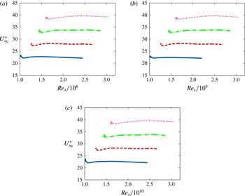
Figure 1 shows
 $U_{\infty }^{+}$
versus
 $Re_{x}$
for a series of higher-resolution (
 $BH$
,
 $CH$
,
 $DH$
) LES runs at different
 $\unicode[STIX]{x1D6FC}$
and at different inlet Reynolds numbers. Three ranges of
 $Re_{x}$
– lower, intermediate and higher – are shown for each
 $\unicode[STIX]{x1D6FC}$
. For all cases, the results displayed begin at the recycling plane and extend downstream. For all runs, some effect of the recycling region
 $0\leqslant x/L_{x}\leqslant 0.2$
can be seen just downstream of the recycling plane. As
 $Re_{x}$
increases,
 $U_{\infty }^{+}$
remains almost constant for each
 $\unicode[STIX]{x1D6FC}$
but at levels that vary with
 $\unicode[STIX]{x1D6FC}$
. In this sense these figures can be interpreted as essentially the fully rough large-Reynolds-number limit for the zero-pressure-gradient boundary layer flowing over roughness whose scale increases linearly with
 $x$
.
Velocity ratio
 $U_{\infty }^{+}$
for a range of
 $Re_{x}$
. Results represent individual LES over different
 $Re_{x}$
: (a) lower range, (b) intermediate range, (c) upper range. Results plotted are for cases
 $\mathit{BH}$
,
 $\mathit{CH}$
and
 $\mathit{DH}$
. Line key: ——,
 $\unicode[STIX]{x1D6FC}=10^{-4}$
; – – –,
 $\unicode[STIX]{x1D6FC}=10^{-5}$
; – - – -,
 $\unicode[STIX]{x1D6FC}=10^{-6}$
;
 $\cdots \cdots$
,
 $\unicode[STIX]{x1D6FC}=10^{-7}$
. Note increasing
 $U_{\infty }^{+}$
with decreasing
 $\unicode[STIX]{x1D6FC}$
.

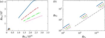
The corresponding variation of
 $Re_{\unicode[STIX]{x1D703}}$
with distance
 $x$
is displayed in figure 2 in both linear–linear (a) and log–log (b) form. Figure 2(a) indicates that all curves appear to converge to the same virtual leading edge, independent of
 $\unicode[STIX]{x1D6FC}$
. A plot of
 $Re_{\unicode[STIX]{x1D6FF}\ast }$
versus
 $Re_{x}$
(not shown) shows similar trends. In figure 2 some domain end effects can be seen for all LES. These are most pronounced for the largest value of
 $\unicode[STIX]{x1D6FC}$
. Both plots clearly indicate an approximately linear growth of
 $Re_{\unicode[STIX]{x1D703}}$
with slopes that depend on
 $\unicode[STIX]{x1D6FC}$
but that appear sensibly independent of
 $Re_{x}$
. Together, these plots indicate an asymptotic state of the boundary layer at large
 $Re_{x}$
that depends on the single parameter
 $\unicode[STIX]{x1D6FC}$
.
Plots of
 $Re_{\unicode[STIX]{x1D703}}$
versus
 $Re_{x}$
with linear–linear (a) and log–log (b) axes. Results represent individual LES over different
 $Re_{x}$
for cases
 $\mathit{BH}$
,
 $\mathit{CH}$
and
 $\mathit{DH}$
. See figure 1 for key; — ⋅ ⋅ —,
 $Re_{\unicode[STIX]{x1D703}}\sim Re_{x}$
.

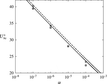
In the following comparisons, all model calculations use
 $\unicode[STIX]{x1D705}=0.384$
,
 $B=8.5$
and
 $\unicode[STIX]{x1D6F1}=0.36$
,
 $0.55$
. Plots of average values of
 $U_{\infty }^{+}$
,
 $\unicode[STIX]{x1D703}/x$
and
 $\unicode[STIX]{x1D6FF}_{99}/x$
obtained from the LES are displayed in figures 3 and 4, respectively. Both high- (HR) and low-resolution (LR) runs are shown for cases
 $C$
and
 $D$
(intermediate and large
 $Re_{x}$
range). The LES values shown as symbols were obtained by streamwise averaging from
 $x^{\prime }/L_{x}=0.2$
to
 $x^{\prime }/L_{x}=0.90$
in order to avoid effects of the outlet boundary condition. In each figure, the solid and dashed lines indicate values derived from the model of § 2.2 over a continuous range of
 $\unicode[STIX]{x1D6FC}$
for the parameter values shown in the caption. In figure 3, both the lower- and higher-resolution LES shows good agreement for
 $U_{\infty }^{+}$
with the model predictions for both values of
 $\unicode[STIX]{x1D6F1}$
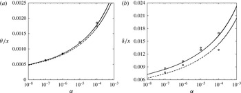
. The agreement between the model and LES results for
 $\overline{\unicode[STIX]{x1D703}}/x$
in figure 4(a) is also good. In figure 4(b) we have plotted
 $\unicode[STIX]{x1D6FF}_{99}/x$
for the LES and
 $\unicode[STIX]{x1D6FF}$
defined by the log-wake law for the model. We note that Squire et al. (Reference Squire, Morrill-Winter, Hutchins, Schultz, Klewicki and Marusic2016) suggest
 $\unicode[STIX]{x1D6FF}=1.26\unicode[STIX]{x1D6FF}_{99}$
but this is not used presently. Overall, figures 1–4 indicate that the LES shows similar trends with acceptable quantitative agreement with the semi-empirical model. At large
 $Re_{x}$
, decreasing
 $\unicode[STIX]{x1D6FC}$
leads to increased
 $U_{\infty }^{+}$
but slower streamwise boundary-layer growth.
Friction velocity ratio
 $U_{\infty }^{+}$
versus
 $\unicode[STIX]{x1D6FC}$
for HR-LES (▫) and LR-LES (○). Solid line: model of § 2.2 with
 $\unicode[STIX]{x1D705}=0.384$
,
 $B=8.5$
and
 $\unicode[STIX]{x1D6F1}=0.55$
. Dashed line: model with
 $\unicode[STIX]{x1D705}=0.384$
,
 $B=8.5$
and
 $\unicode[STIX]{x1D6F1}=0.36$
. Symbols indicate values obtained from LES via averaging from
 $x^{\prime }/L_{x}=0.2$
to
 $x^{\prime }/L_{x}=0.90$
in order to avoid effects of the outlet boundary condition. Cases
 $\mathit{CH}$
and
 $\mathit{DH}$
.

Plots of
 $\unicode[STIX]{x1D703}/x$
versus
 $\unicode[STIX]{x1D6FC}$
(a) and
 $\unicode[STIX]{x1D6FF}/x$
versus
 $\unicode[STIX]{x1D6FC}$
(b). For key, see figure 3. LES results represent
 $\unicode[STIX]{x1D6FF}_{99}$
versus
 $\unicode[STIX]{x1D6FC}$
.

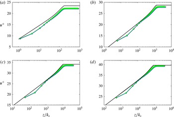
Figure 5 shows mean-velocity profiles
 $u(z)/\overline{u}_{\unicode[STIX]{x1D70F}}$
versus
 $z/(\unicode[STIX]{x1D6FC}x)$
for
 $\unicode[STIX]{x1D6FC}=10^{-4}$
,
 $10^{-5}$
,
 $10^{-6}$
and
 $10^{-7}$
. For each value of
 $\unicode[STIX]{x1D6FC}$
, four velocity profiles at streamwise stations indicated in the figure caption are plotted. Reasonable collapse at each
 $\unicode[STIX]{x1D6FC}$
is indicated. The LES show small near-wall effects in the final three near-wall grid points. Also shown in each panel is the model mean-velocity profile (2.17). These use the values of
 $\unicode[STIX]{x1D6FC}$
shown together with
 $\unicode[STIX]{x1D705}=0.384$
,
 $B=8.5$
and
 $\unicode[STIX]{x1D6F1}=0.55$
. The model profile shows slightly higher
 $U_{\infty }/u_{\unicode[STIX]{x1D70F}}$
than the LES profile for each
 $\unicode[STIX]{x1D6FC}$
consistent with the differences between results from the semi-empirical model and the LES shown in figure 3.
Mean velocity profiles
 $u^{+}$
versus
 $z/k_{s}=z/(\unicode[STIX]{x1D6FC}x)$
at four streamwise stations for each
 $\unicode[STIX]{x1D6FC}$
as shown: (a)
 $\unicode[STIX]{x1D6FC}=10^{-4}$
, (b)
 $\unicode[STIX]{x1D6FC}=10^{-5}$
, (c)
 $\unicode[STIX]{x1D6FC}=10^{-5}$
, (d)
 $\unicode[STIX]{x1D6FC}=10^{-7}$
. Results plotted are for cases
 $\mathit{CH}$
. Symbols represent different streamwise stations. See table 6 for key. Solid line: equation (2.17) with
 $\unicode[STIX]{x1D705}=0.384$
,
 $B=8.5$
and
 $\unicode[STIX]{x1D6F1}=0.55$
.

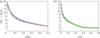
In figure 6 the defect velocity
 $(u-U_{\infty })/\overline{u}_{\unicode[STIX]{x1D70F}}$
is plotted against both
 $z/\unicode[STIX]{x1D6FF}_{99}$
and
 $z/\unicode[STIX]{x1D6E5}$
. One profile for each of the four values of
 $\unicode[STIX]{x1D6FC}$
is plotted. Equations (2.3) and (2.4) together suggest that
 $U_{\infty }^{+}-u^{+}$
is a function of
 $z/\unicode[STIX]{x1D6FF}_{99}$
independent of
 $\unicode[STIX]{x1D6FC}$
provided we identify
 $\unicode[STIX]{x1D6FF}=\unicode[STIX]{x1D6FF}_{99}$
. This is because the
 $-\log (k_{s})/\unicode[STIX]{x1D705}$
terms cancel. That
 $U_{\infty }^{+}-u^{+}$
can also be expressed as a function of
 $z/\unicode[STIX]{x1D6E5}$
independent of
 $\unicode[STIX]{x1D6FC}$
is suggested by the constancy of the ratio
 $\unicode[STIX]{x1D6E5}/\unicode[STIX]{x1D6FF}_{99}=3.54$
across all
 $\unicode[STIX]{x1D6FC}$
in the LES and also from the model equation (2.9) that does not depend explicitly on
 $\unicode[STIX]{x1D6FC}$
. Figure 6(b) shows reasonable collapse against
 $z/\unicode[STIX]{x1D6E5}$
. The collapse is not as good against
 $z/\unicode[STIX]{x1D6FF}_{99}$
in figure 6(a) where small effects of
 $\unicode[STIX]{x1D6FC}$
can be seen.
Velocity defect
 $(U_{\infty }-u)/u_{\unicode[STIX]{x1D70F}}$
for a range of roughness slopes
 $\unicode[STIX]{x1D6FC}$
versus the wall-normal coordinate
 $z$
: (a) versus
 $z/\unicode[STIX]{x1D6FF}_{99}$
; (b) versus
 $z/\unicode[STIX]{x1D6E5}$
with Rotta–Clauser parameter
 $\unicode[STIX]{x1D6E5}=U_{\infty }\unicode[STIX]{x1D6FF}^{\ast }/u_{\unicode[STIX]{x1D70F}}$
. Single streamwise station for each
 $\unicode[STIX]{x1D6FC}$
shown for clarity. Symbol key: ▪,
 $\unicode[STIX]{x1D6FC}=10^{-4}$
; ●,
 $\unicode[STIX]{x1D6FC}=10^{-5}$
; ▲ ,
 $\unicode[STIX]{x1D6FC}=10^{-6}$
; ▼,
 $\unicode[STIX]{x1D6FC}=10^{-7}$
.

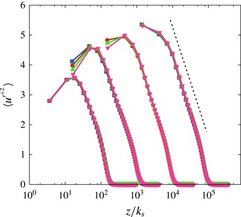
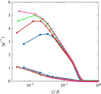
Streamwise velocity variances
 $\langle u^{\prime +2}\rangle \equiv \overline{u^{\prime 2}}/\overline{u}_{\unicode[STIX]{x1D70F}}^{2}$
obtained from the LES are shown in figures 7 and 8. In figure 7, these are plotted against
 $z/(\unicode[STIX]{x1D6FC}x)$
. Again, four streamwise stations are shown in each plot. The three near-wall points are probably affected by the wall modelling and cannot be considered accurate. While the effect of
 $\unicode[STIX]{x1D6FC}$
can clearly be seen in the separation of the profiles when plotted against
 $z/k_{s}=z/(\unicode[STIX]{x1D6FC}x)$
, each profile appears to have approximately the same slope in linear–log coordinates. For the turbulent boundary layer over a uniformly rough wall, Squire et al. (Reference Squire, Morrill-Winter, Hutchins, Schultz, Klewicki and Marusic2016) find an approximately logarithmic profile for streamwise velocity variances with slope
 $A_{1}\approx 1.27$
. Figure 7 suggests the form
 $\langle u^{\prime +2}\rangle =B_{1}(\unicode[STIX]{x1D6FC})-A_{1}\log (z/k_{s})$
where
 $A_{1}$
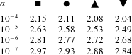
is independent of
 $\unicode[STIX]{x1D6FC}$
. The light solid line in figure 7 has slope
 $A_{1}\approx 1.60$
. In figure 8,
 $\langle u^{\prime +2}\rangle$
is plotted against
 $z/\unicode[STIX]{x1D6E5}$
, with some degree of collapse over the outer region. The profiles shown in both figures 7 and 8 comprise the sum of the resolved-scale component plus the subgrid component obtained from the SGS model. The latter are shown in figure 8, where they are small but not negligible.
Streamwise velocity fluctuations
 $\langle u^{\prime +2}\rangle =\overline{u^{\prime 2}/u_{\unicode[STIX]{x1D70F}}^{2}}$
. Four streamwise stations for each
 $\unicode[STIX]{x1D6FC}$
shown. Note
 $\unicode[STIX]{x1D6FC}$
decreasing left to right. Dashed line is of the form
 $\langle u^{\prime +2}\rangle =B_{1}-A_{1}\log (z/k_{s})$
with
 $A_{1}=1.60$
. See table 6 for key.

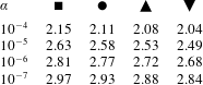
Symbol key for plots with multiple streamwise stations. Stations identified by
 $Re_{x}/10^{9}$
.
Streamwise velocity fluctuations
 $\langle u^{\prime +2}\rangle =\overline{u^{\prime 2}/u_{\unicode[STIX]{x1D70F}}^{2}}$
versus
 $z/\unicode[STIX]{x1D6E5}$
. One streamwise station for each
 $\unicode[STIX]{x1D6FC}$
shown for clarity. Both subgrid and total (subgrid plus resolved-scale) results shown. See figure 6 for symbol key.

6 Conclusions
A semi-empirical model has been developed that describes the development of a class of fully turbulent boundary layers at large Reynolds numbers over roughness that varies linearly with streamwise distance. For fixed values of the von Kármán constant, the Coles wake factor and the offset parameter, the model contain two parameters. The first is the exponent
 $m$
in the outer-flow velocity profile, while the second is the dimensionless slope of the roughness-scale variation with distance
 $\unicode[STIX]{x1D6FC}$
. The model is predicated on the ansatz that all terms in the von Kármán integral relationship are constant in the streamwise direction. This is found to be consistent with constant
 $U_{\infty }^{+}$
and with all defined measures of the boundary-layer thickness growing linearly with streamwise distance. For given
 $m$
and
 $\unicode[STIX]{x1D6FC}$
, both the streamwise and the wall-normal components of the mean velocity depend only on the single similarity variable
 $z/(\unicode[STIX]{x1D6FC}x)$
. Two interesting flows that approximately satisfy the model conditions are the zero-pressure-gradient boundary layer,
 $m=0$
, and pure sink flow,
 $m=-1$
.
Large-eddy simulations have been performed for the zero-pressure-gradient boundary-layer flow using a wall modelled region that incorporates a simple semi-empirical model of subgrid wall roughness. This roughness model is local and allows linear growth of the roughness scale with streamwise distance. Utilizing a recycling technique for creating appropriate turbulent inflow boundary conditions and employing an iteration method to ensure that the virtual origin of both the boundary-layer growth and the roughness-scale variation coincide, for given
 $\unicode[STIX]{x1D6FC}$
, the LES produces a statistically steady boundary-layer flow. At sufficiently large Reynolds number
 $Re_{x}$
, the displacement, momentum and the 99 % velocity thicknesses all grow approximately linearly with streamwise distance while
 $U_{\infty }^{+}$
becomes constant. Comparison of the LES and semi-empirical model results for some mean measures of the boundary-layer development show similar qualitative and quantitative trends. Both the mean-velocity profiles and the streamwise mean-square velocity fluctuations obtained from the LES show self-similar scaling on the length scale
 $k_{s}=\unicode[STIX]{x1D6FC}x$
with dependence on
 $\unicode[STIX]{x1D6FC}$
. The velocity defect profiles show reasonable collapse using the Rotta–Clauser length scale independent of
 $\unicode[STIX]{x1D6FC}$
.
In the sense that
 $U_{\infty }^{+}$
, or equivalently the surface skin-friction coefficient, remains streamwise constant, both the semi-empirical model and the LES can be interpreted as representing the fully rough limit of a Moody-like diagram for the zero-pressure-gradient boundary-layer flow. Since the present model indicates a range of admissible values of
 $m$
, the present work suggests the existence of a class of Moody-like diagrams for turbulent boundary-layer flows in the presence of linear streamwise variation in surface roughness.
Acknowledgements
A.S. and D.I.P. were partially supported by the KAUST Office of Competitive Research Funds (OCRF) under award no. URF/1/1394-01 and partially by NSF award CBET 1235605. W.C. was supported by the KAUST OCRF under award no. URF/1/1394-01. The authors acknowledge helpful conversations with R. A. Antonia.