1 Introduction
Particle-laden fluids, or suspensions, occur in natural phenomena such as blood flow as well as applications including cement mixing and slurry transport of coal. While a great deal of effort has been devoted to the determination of the rheological description of suspensions, particularly under viscously dominated conditions, prediction of the behaviour of suspensions under the varied conditions encountered in these contexts requires consideration of inertial flow phenomena, and this aspect of suspension mechanics remains largely undeveloped. Here, we experimentally probe the behaviour of suspensions in concentric cylinders, i.e. Taylor–Couette flow (TCF), which has been comprehensively studied for pure fluids, to explore how inertial transitions are influenced by suspended particles. To maintain a relatively homogeneous mixture, we consider neutrally buoyant suspensions, with density matching of particles and liquid, yet the notion of treating the suspension as a homogeneous material with an effective viscosity does not map the behaviour to that known for the pure fluid. Known flow transitions are consistently altered by particle loading, while the particles make qualitative changes to the characteristics of the TCF as a dynamical system.
The classic Taylor–Couette flow, with long axial extent relative to the annular gap, depends upon the ratio
 $\unicode[STIX]{x1D702}=d_{i}/d_{o}$
where
 $d_{i}$
and
 $d_{o}$
are, respectively, the inner and outer cylinder diameters, as well as the rates of rotation of the inner and outer cylinders. At sufficient rotational velocity of the inner cylinder, the simple circular motion becomes unstable to pairs of counter-rotating vortices if the outer cylinder is stationary, while spirals may be seen as the first transition if the outer cylinder is rotating in the opposite direction to the inner (Andereck, Liu & Swinney Reference Andereck, Liu and Swinney1986). For simplicity, we fix
 $\unicode[STIX]{x1D702}$
and rotate only the inner cylinder, allowing a focus on the influence of the additional parameters resulting from introduction of the particles: (i) the size of the particles compared to the annular width; (ii) the particle volume fraction, denoted
 $\unicode[STIX]{x1D719}$
; (iii) the Reynolds number,
 $Re=(d_{o}-d_{i})\unicode[STIX]{x1D6FA}_{i}d_{i}\unicode[STIX]{x1D70C}/4\unicode[STIX]{x1D707}_{s}$
, characterizing the bulk flow, here defined using the measured effective viscosity of the suspension. Here
 $\unicode[STIX]{x1D6FA}_{i}$
is the rotation rate of the inner cylinder and
 $\unicode[STIX]{x1D70C}$
is the density of the suspension. The particles used here are large enough to neglect Brownian effects.
At low Reynolds number, particles in dilute suspension flows follow streamlines. However, at higher concentrations, hydrodynamic interactions between particles lead to self-diffusion in uniform flows and shear-induced migration in non-uniform shear flows (Da Cunha & Hinch Reference Da Cunha and Hinch1996; Drazer et al.
Reference Drazer, Koplik, Khusid and Acrivos2002; Stickel & Powell Reference Stickel and Powell2005). Shear-induced migration results in heterogeneous concentration fields and modified velocity profiles (Cox & Mason Reference Cox and Mason1971; Abbott et al.
Reference Abbott, Tetlow, Graham, Altobelli, Fukushima, Mondy and Stephens1991; Graham et al.
Reference Graham, Altobelli, Fukushima, Mondy and Stephens1991; Koh, Hookham & Leal Reference Koh, Hookham and Leal1994). Migration due to inertia must also be considered. At finite
 $Re$
in dilute suspension flows, interaction of particle disturbances with the background flow leads to inertial migration of the particles to specific locations in the flow cross-section (Segré & Silberberg Reference Segré and Silberberg1962; Schonberg & Hinch Reference Schonberg and Hinch1989; Asmolov Reference Asmolov1999; Matas, Morris & Guazzelli Reference Matas, Morris and Guazzelli2009; Miura, Itano & Sugihara-Seki Reference Miura, Itano and Sugihara-Seki2014). At intermediate and high concentrations, the particle–particle hydrodynamic interactions along with inertial migration leads to non-uniform concentration profiles and hence modified velocity fields (Han et al.
Reference Han, Kim, Kim and Lee1999). In the present work, we are careful to avoid conditions which would allow for extended periods of simple shear of the suspension which would lead to such heterogeneity.
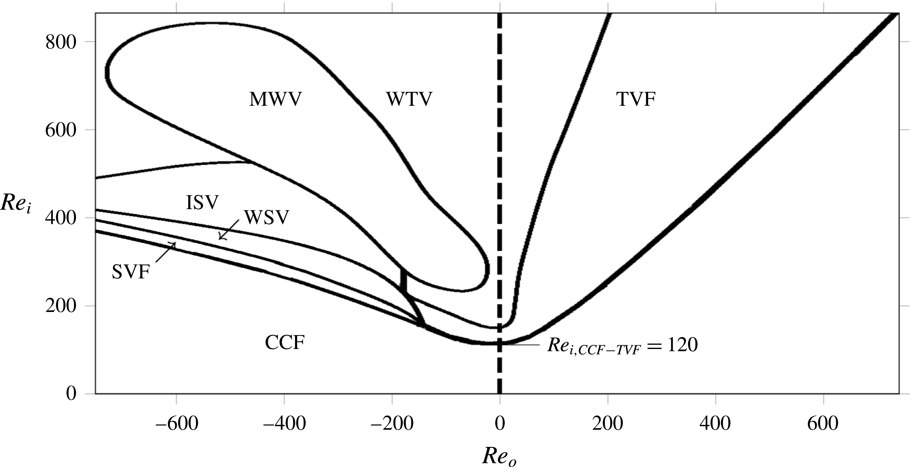
Flow structures of pure fluid in an annulus between two independently rotating concentric cylinders with ratio of inner to outer cylinder radius
 $\unicode[STIX]{x1D6E4}=d_{i}/d_{o}=0.88$
: CCF-circular Couette flow, SVF-spiral vortex flow, TVF-Taylor vortex flow, WTV-wavy Taylor vortices, WSV-wavy spiral vortices, ISV-interpenetrating spiral vortices and MWV-modulated wavy vortices. Here,
 $Re_{i}$
and
 $Re_{o}$
are the Reynolds numbers based on inner and outer cylinder rotation rates, respectively. Adapted from Andereck et al. (Reference Andereck, Liu and Swinney1986). The present study with suspension probes flow structures at conditions along the vertical dashed line (
 $Re_{o}=0$
,
 $Re_{i}>0$
) only.

Study of inertial flow transitions in suspensions has been considered in pipe and other conduit flows. Experiments by Matas, Morris & Guazzelli (Reference Matas, Morris and Guazzelli2003) showed that density matched particles in Poiseuille flow lower the
 $Re$
for the laminar–turbulent flow transition, with the influence amplified with increase in particle size and
 $\unicode[STIX]{x1D719}$
, e.g. for particles of one tenth of the tube diameter, values of
 $Re\approx 800$
were found at
 $\unicode[STIX]{x1D719}=0.08$
and above. The rescaling of the Reynolds number to account for the added dissipation due to the particles was found to be effective only if the particles were smaller than 1/60th of the tube diameter. Numerical simulations of Loisel et al. (Reference Loisel, Abbas, Masbernat and Climent2013) using the force coupling method (Lomholt & Maxey Reference Lomholt and Maxey2003) predict lower
 $Re$
corresponding to laminar–turbulent transition for a channel flow of suspension (
 $\unicode[STIX]{x1D719}=0.05$
). It was reported that this transition
 $Re$
reduction is due to finite-size particles inducing local perturbations and breaking large-scale eddies into smaller and more energetic vortical structures.
While it is a practically very important flow and has aroused intense scientific interest, the pipe flow undergoes a subcritical transition as the laminar flow is linearly stable at all
 $Re$
, and this makes it a challenging environment to explore inertial flow transitions. By contrast, linear stability theory provides valuable guidance to the flow transitions between rotating concentric cylinders, i.e. the Taylor–Couette flow. The various flow transitions in TCF have been studied extensively for many years (Taylor Reference Taylor1923; Chandrasekhar Reference Chandrasekhar1958; Coles Reference Coles1965) with both experimental and theoretical approaches, and more recently using numerical simulation (Czarny et al.
Reference Czarny, Serre, Bontoux and Lueptow2002; Hoffmann, Lücke & Pinter Reference Hoffmann, Lücke and Pinter2004). Andereck et al. (Reference Andereck, Liu and Swinney1986) compiled the flow structures corresponding to the Reynolds numbers based on inner and outer cylinder rotation rates:
 $(Re_{i},Re_{o})=\unicode[STIX]{x1D6FF}(\unicode[STIX]{x1D6FA}_{i}d_{i},\unicode[STIX]{x1D6FA}_{o}d_{o})\unicode[STIX]{x1D70C}/2\unicode[STIX]{x1D707}$
where
 $\unicode[STIX]{x1D6FF}$
is the annular gap,
 $d_{i}$
and
 $d_{o}$
are the diameters of the inner and outer cylinders,
 $\unicode[STIX]{x1D6FA}_{i}$
and
 $\unicode[STIX]{x1D6FA}_{o}$
are the rotation rates of inner and outer cylinders and
 $\unicode[STIX]{x1D70C}$
and
 $\unicode[STIX]{x1D707}$
are the density and viscosity of the Newtonian fluid (refer to figure 1). Within the ranges of
 $Re_{i}$
and
 $Re_{o}$
shown in figure 1, for
 $Re_{o}>-135$
and slow increase of
 $Re_{i}$
(including the cases of rotating cylinders with small counter-rotation, fixed outer and rotating inner cylinder and co-rotating cylinders), the flow transitions from circular Couette flow (CCF) to Taylor vortex flow (TVF) to wavy Taylor vortices (WTV). For
 $Re_{o}<-135$
, the flow goes through several transitions: from circular Couette flow to spiral vortex flow (SVF) to wavy spiral vortices (WSV) to interpenetrating spiral vortices to modulated waves to wavy Taylor vortices. The TCF is thus a fertile ground for examination of instability phenomena. Inertial elastic instabilities and pure elastic instabilities in Taylor–Couette flow have been studied in detail (Larson, Shaqfeh & Muller Reference Larson, Shaqfeh and Muller1990; Muller, Shaqfeh & Larson Reference Muller, Shaqfeh and Larson1993; Baumert & Muller Reference Baumert and Muller1995; Martínez-Arias & Peixinho Reference Martínez-Arias and Peixinho2017). Taylor–Couette instabilities in ferrofluids, suspensions of ferromagnetic nanoparticles, under external magnetic fields have been explored (Odenbach & Gilly Reference Odenbach and Gilly1996; Altmeyer et al.
Reference Altmeyer, Hoffmann, Leschhorn and Lücke2010). A few studies have investigated the effect of finite-size particles on the flow transitions, with Ali et al. (Reference Ali, Mitra, Schwille and Lueptow2002) an example in which linear stability analysis predicted that the particles destabilize the circular Couette flow for a non-Brownian suspension in the dilute limit (
 $\unicode[STIX]{x1D719}<0.05$
). However, in this same study, experiments with neutrally buoyant particles (gap to particle ratio of
 $250$
) for concentrations
 $\unicode[STIX]{x1D719}<0.005$
showed a stabilizing effect of the particles, in contrast to the predictions. More recently, experiments by Dherbécourt et al. (Reference Dherbécourt, Charton, Lamadie, Cazin and Climent2016) showed improved mixing in Taylor vortex flow (TVF) by the addition of particles. They used neutrally buoyant particles of size
 $d_{p}=800{-}1500~\unicode[STIX]{x03BC}\text{m}$
(gap to particle ratio of 13.75–7.3) in volume fractions between
 $0.01\leqslant \unicode[STIX]{x1D719}\leqslant 0.08$
.
In the present study, we investigate the effect of particle loading and size on the flow transitions and flow structures of neutrally buoyant suspensions sheared between a rotating inner cylinder and stationary outer cylinder, the condition lying along the vertical dashed line (
 $Re_{o}=0$
,
 $Re_{i}>0$
) in figure 1. Flow structures observed for pure fluid along this line are CCF, TVF and WTV. For the suspension, in addition to CCF, TVF and WTV, we observe non-axisymmetric flow structures including ribbons (RIB), SVF and WSV. We give the details of the experimental geometry and materials used in § 2. Experiments with pure fluid are reported in § 3.1 as part of the calibration of the apparatus. In § 3.2, we detail the protocol used for the suspension experiments. Experimental observations for the
 $\unicode[STIX]{x1D719}=0.10$
suspension are discussed in detail in § 3.3. In § 3.5 the full experimental observations for suspensions of
 $0\leqslant \unicode[STIX]{x1D719}\leqslant 0.30$
are presented, followed by conclusions in § 4.
2 Experimental apparatus and materials
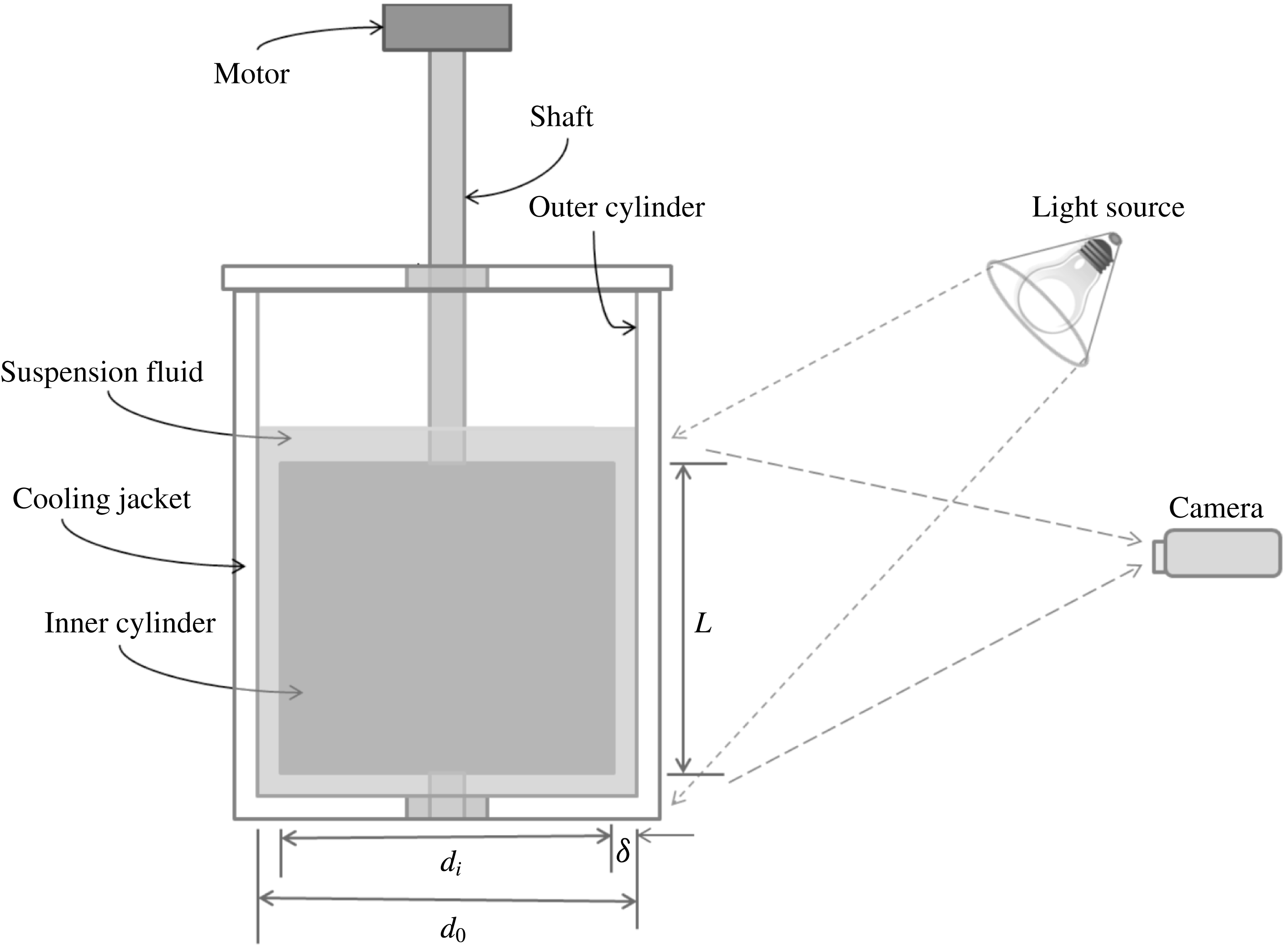
The primary experimental apparatus consists of two vertical coaxial cylinders, as shown in figure 2. The surface of the inner solid aluminium cylinder is uniformly coated with non-reflective black paint for better visualization. The inner cylinder is
 $100.3$
mm in diameter (
 $d_{i}$
) and
 $144$
mm in length (
 $L$
). The outer transparent acrylic cylinder is
 $114.3$
mm in diameter (
 $d_{o}$
). The resulting annular gap,
 $\unicode[STIX]{x1D6FF}=(d_{o}-d_{i})/2=7~\text{mm}$
. The end plates are affixed to the outer cylinder and in each of these horizontal plates ball bearings are mounted at the centre. A shaft holding the inner cylinder along its axis sits in the bottom ball bearing and keeps the inner cylinder
 $1$
mm above the lower end plate. The top part of the shaft passes through the top ball bearing and is connected to a stepper motor using a flexible coupling. This arrangement allows free rotation of the inner cylinder while maintaining axial alignment. A MATLAB-based computer interface was used to control the angular velocity (
 $\unicode[STIX]{x1D6FA}$
) and acceleration at which the stepper motor rotates the inner cylinder. The outer cylinder is held fixed. A rectangular transparent cooling jacket was built around the outer cylinder using acrylic material. Water at
 $20\,^{\circ }\text{C}$
was circulated through the cooling jacket for the duration of the experiment to maintain a constant suspension temperature.
Schematic of the experimental set-up.

The working fluid is a neutrally buoyant suspension of non-Brownian spherical particles. The particles are made of poly-(methyl methacrylate), or PMMA, with density
 $1.18~\text{g}~\text{cm}^{-3}$
. To study the particle size effect on the flow transitions, particles of two sizes were used: (i) diameter in the range
 $212\leqslant d_{p}\leqslant 250~\unicode[STIX]{x03BC}\text{m}$
(mean
 $d_{p}\approx 230~\unicode[STIX]{x03BC}\text{m}$
) and (ii)
 $d_{p}\approx 70~\unicode[STIX]{x03BC}\text{m}$
, obtained by sieving in each case. To study the effect of particle concentration on the flow transitions, the particle volume fraction was varied over
 $0\leqslant \unicode[STIX]{x1D719}\leqslant 0.30$
. To narrow the density range, the particles were combined with a mixture of water and glycerol in
 $1:2$
weight ratio and left overnight. Those particles that stayed suspended in the fluid were separated, washed and dried before use in the experiments. In this way, we achieved good neutral buoyancy of the particles in the suspension. In each experiment, the suspending fluid was prepared by mixing water and glycerol of
 $1:2$
weight ratio to match the fluid density to that of the particles at
 $20\,^{\circ }\text{C}$
. A small quantity (
 $0.04$
% by volume) of the surfactant Triton X-100 (Sigma Aldrich) was added to the suspension to avoid particle adhesion to the air–water interface.
For the purpose of visualization of flow structures,
 $0.05$
% by volume of Pearl Swirl (Steve Spangler Science) made of
 $1$
% by volume of flakes in aqueous solution was added to the fluid mixture; these flakes are a proprietary mixture of titanium dioxide and crystalline silica and are
 $12~\unicode[STIX]{x03BC}\text{m}$
in the largest dimension and much thinner in the perpendicular dimension. When illuminated from the top at an angle as shown in figure 2, the flakes reflect light toward the camera at different intensities depending on their orientation in the flow field. This variation in the reflected light intensity is recorded by two cameras for each experiment: (i) a high speed camera (Photron FASTCAM 1024 PCI) to record
 $60~\text{frames}~\text{s}^{-1}$
for short durations (up to 10 s), and (ii) a low speed camera (Dino-Lite) to record at less than
 $1~\text{frame}~\text{s}^{-1}$
for durations up to a few hours.
Particles and suspending fluid were mixed to make suspensions of the desired concentration, and
 $500$
ml was placed inside the annulus to submerge the inner cylinder by
 $18$
mm. The fluid was left overnight with small inner cylinder rotation to separate any air bubbles before starting the experiment.
3 Results and discussion
The non-dimensional parameters characterizing the materials and the apparatus are the particle volume fraction
 $0\leqslant \unicode[STIX]{x1D719}\leqslant 0.30$
, the ratio of inner and outer diameters (
 $\unicode[STIX]{x1D702}=d_{i}/d_{o}=0.877$
), the annulus length relative to the annular gap (
 $\unicode[STIX]{x1D6E4}=L/\unicode[STIX]{x1D6FF}=20.5$
) and ratio of annular gap to the particle diameter (
 $\unicode[STIX]{x1D6FC}=\unicode[STIX]{x1D6FF}/d_{p}=30$
and
 $100$
). The Reynolds number is defined as
 $Re=\unicode[STIX]{x1D6FF}d_{i}\unicode[STIX]{x1D6FA}\unicode[STIX]{x1D70C}/2\unicode[STIX]{x1D707}_{s}$
. Here
 $\unicode[STIX]{x1D6FA}$
is the angular velocity of the inner cylinder and
 $\unicode[STIX]{x1D70C}$
and
 $\unicode[STIX]{x1D707}_{s}$
are the density and the effective bulk viscosity of the suspension, respectively. A rheometer (AR 2000ex TA Instruments) with parallel plate fixture (
 $50$
mm plate diameter and
 $1.5$
mm gap) was used to measure the effective viscosity of the suspension,
 $\unicode[STIX]{x1D707}_{s}$
. At each concentration between
 $\unicode[STIX]{x1D719}=0$
and
 $\unicode[STIX]{x1D719}=0.30$
, viscosity measurements were made at five different shear rates between
 $\dot{\unicode[STIX]{x1D6FE}}=20$
and
 $\dot{\unicode[STIX]{x1D6FE}}=100~\text{s}^{-1}$
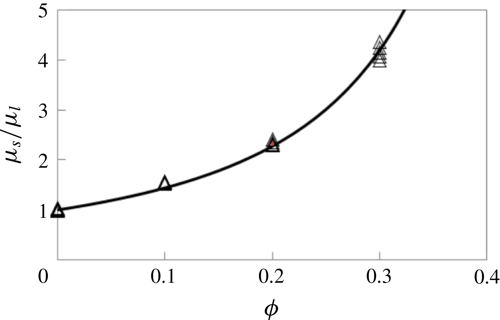
and plotted in figure 3. Measured suspension viscosities for particle volume fractions
 $0\leqslant \unicode[STIX]{x1D719}\leqslant 0.30$
followed very closely the Krieger correlation,
 $\unicode[STIX]{x1D707}_{s}=\unicode[STIX]{x1D707}_{l}(1-\unicode[STIX]{x1D719}/\unicode[STIX]{x1D719}_{m})^{-1.82}$
with
 $\unicode[STIX]{x1D719}_{m}=0.55$
, where
 $\unicode[STIX]{x1D707}_{l}$
is the viscosity of the fluid mixture without particles.
Dependence of the suspension viscosity on the particle concentration. Open triangles represent the experimental measurements and the solid line represents the correlation,
 $\unicode[STIX]{x1D707}_{s}/\unicode[STIX]{x1D707}_{l}=(1-\unicode[STIX]{x1D719}/\unicode[STIX]{x1D719}_{m})^{-1.82}$
with
 $\unicode[STIX]{x1D719}_{m}=0.55$
.

To observe flow structures corresponding to various
 $Re$
in the Taylor–Couette geometry, the standard method followed in most prior work is the increasing-
 $Re$
ramp protocol in which
 $Re$
is increased to observe flow transitions: i.e. one starts with a stationary inner cylinder, increasing the inner cylinder
 $Re$
with time
 $t$
with a small acceleration (i.e. in a quasi-steady manner) so that the steady state flow structures are accessed at all times (Taylor Reference Taylor1923; Chandrasekhar Reference Chandrasekhar1958; Coles Reference Coles1965). A non-dimensional acceleration defined as
 $\text{d}Re/\text{d}\unicode[STIX]{x1D70F}$
can be used as the measure of the ramp rate. Here the time is non-dimensionalized as
 $\unicode[STIX]{x1D70F}=t/t_{d}$
using a diffusion time scale
 $t_{d}=(\unicode[STIX]{x1D6FF}^{2}\unicode[STIX]{x1D70C})/\unicode[STIX]{x1D707}_{s}$
. A value of
 $\text{d}Re/\text{d}\unicode[STIX]{x1D70F}\ll 1$
ensures no effect of acceleration on the results (Dutcher & Muller Reference Dutcher and Muller2009).
3.1 Calibration with pure fluid
To calibrate the experimental apparatus, the annulus was filled with pure fluid for which the diffusion time scale is
 $t_{d}\approx 2.1~\text{s}$
. The inner cylinder rotation was increased quickly from rest to
 $Re=90$
and held at this condition for
 $20$
minutes to establish a steady circular Couette flow (CCF) in the annulus. The
 $Re$
was then increased slowly at a rate of
 $\text{d}Re/\text{d}t=0.0061~\text{s}^{-1}$
(
 $\text{d}Re/\text{d}\unicode[STIX]{x1D70F}=0.013$
) to
 $Re=210$
. The flow structures during this
 $5.5$
hour experiment were photographed using the low speed camera at an interval of 50 s between frames. At regular intervals, photographs for short durations (
 $t=2.2~\text{s}$
) at a rate of
 $60~\text{frames}~\text{s}^{-1}$
were recorded using the high speed camera.
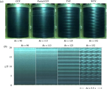
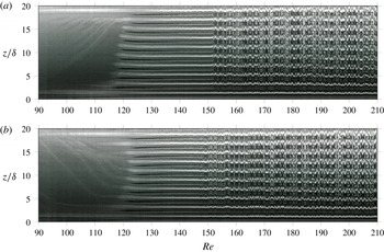
(a) Photographs of the flow structures, and (b) space–time diagrams of CCF, partial CCF, TVF and WTV for pure fluid at
 $Re=90,113,125$
and
 $152$
, respectively, during an increasing-
 $Re$
ramp with
 $\text{d}Re/\text{d}\unicode[STIX]{x1D70F}=0.013$
. The space–time diagrams are constructed from images taken at
 $60~\text{frames}~\text{s}^{-1}$
. Note that at each
 $Re$
in (b), the duration is
 $\unicode[STIX]{x0394}t=2.2~\text{s}$
.

Space–time diagrams constructed from images taken at intervals of 50 s between frames over a
 $5.5$
hour period for pure fluid: (a) during increasing-
 $Re$
ramp from
 $Re=90$
to
 $Re=210$
with
 $\text{d}Re/\text{d}t=0.0061~\text{s}^{-1}$
(
 $\text{d}Re/\text{d}\unicode[STIX]{x1D70F}=0.013$
), and (b) during decreasing-
 $Re$
ramp from
 $Re=210$
to
 $Re=90$
with
 $\text{d}Re/\text{d}t=-0.0061~\text{s}^{-1}$
(
 $\text{d}Re/\text{d}\unicode[STIX]{x1D70F}=-0.013$
). Flow transitioned from CCF to TVF to WTV during the increasing-
 $Re$
ramp and from WTV to TVF to CCF during the decreasing-
 $Re$
ramp.

Figure 4(a) shows four photographs of different flow structures at
 $Re=90$
, 113, 125 and 152. Space–time diagrams, which show the time modulation of the flow structures, are constructed from sequences of such photographs by extracting the light intensity from an area of
 $1$
pixel width (at the centre of the image in the horizontal direction) over the full length of the annulus and plotting it as a function of
 $t$
. Figure 4(b) shows the space–time diagrams at various
 $Re$
, corresponding to the flow structures shown in figure 4(a), constructed from photographs recorded at a rate of
 $60~\text{frames}~\text{s}^{-1}$
for a duration of 2.2 s. Since the slowly ramped
 $Re$
changes negligibly over this time, each space–time diagram constructed from such data represents a particular
 $Re$
. Figure 5(a) shows the space–time diagram constructed from photographs recorded at intervals of 50 s between frames for
 $90\leqslant Re\leqslant 210$
. As the inner cylinder rotation rate at any given time is known, time on the horizontal axis can be replaced by
 $Re$
. At
 $Re=90$
, the flow was observed to be circular Couette flow (CCF) with Ekman rolls near top and bottom boundaries. This flow state was observed to be stable with increase in
 $Re$
. Close to
 $Re=120$
, counter-rotating pairs of Taylor vortices appeared near top and bottom boundaries with a stable CCF in the middle section. These rings eventually filled the whole length of the annulus, transitioning into Taylor vortex flow (TVF) at
 $Re=120$
. This is in agreement with experiments and linear stability theory for the radius ratio of
 $\unicode[STIX]{x1D702}=0.877$
(Andereck et al.
Reference Andereck, Liu and Swinney1986; Recktenwald, Lücke & Müller Reference Recktenwald, Lücke and Müller1993; Ali et al.
Reference Ali, Mitra, Schwille and Lueptow2002). The TVF state was observed to be stable for
 $120\leqslant Re\leqslant 151$
. At
 $Re=151$
, TVF transitioned into wavy Taylor vortices (WTV) in which the vortices oscillate in sinusoidal fashion in the azimuthal direction. With increase in
 $Re$
, the WTV state was observed to be stable up to
 $Re=210$
. The time modulation of CCF, partial CCF, TVF and WTV flow states can be seen in the space–time diagrams at
 $Re=90,113,125$
and
 $152$
, respectively, in figure 4(b).
Figure 5(b) shows the space–time diagram when
 $Re$
was reduced from
 $Re=210$
to
 $Re=90$
at a rate of
 $\text{d}Re/\text{d}t=-0.0061~\text{s}^{-1}$
(
 $\text{d}Re/\text{d}\unicode[STIX]{x1D70F}=-0.013$
). The flow in this decreasing-
 $Re$
ramp experiment was observed to follow the sequence of WTV
 $\rightarrow$
TVF
 $\rightarrow$
CCF. These flow structures at various
 $Re$
and the transition
 $Re$
corresponding to WTV–TVF and TVF–CCF transitions match closely to those observed in the increasing-
 $Re$
ramp, showing no hysteresis in the pure fluid experiments.
3.2 Procedure for experiments with suspension
The objective of the present work is to understand deviations in flow transitions of fluid–particle suspensions compared to those of the pure fluid. The particle concentrations probed in the present work, including the pure fluid (
 $\unicode[STIX]{x1D719}=0$
), are
 $0\leqslant \unicode[STIX]{x1D719}\leqslant 0.30$
for
 $d_{p}\approx 230~\unicode[STIX]{x03BC}\text{m}$
and
 $\unicode[STIX]{x1D719}=0.10$
for
 $d_{p}\approx 70~\unicode[STIX]{x03BC}\text{m}$
. We have applied a protocol in which
 $Re$
was ramped down rather than up for the study of the suspensions. In this protocol, the inner cylinder rotation rate was increased as rapidly as possible from rest to a value of
 $Re$
yielding WTV (typically
 $Re>160$
). Subsequently,
 $Re$
was reduced in a quasi-steady manner with
 $|\text{d}Re/\text{d}\unicode[STIX]{x1D70F}|\ll 1$
until CCF was established in the full length of the annulus. The flow structures were photographed with two cameras as described in § 2. The rationale for not using the standard increasing-
 $Re$
protocol came from a set of experiments we performed with very dilute suspensions (
 $\unicode[STIX]{x1D719}<0.01$
), which showed that an increasing-
 $Re$
ramp could lead to concentration inhomogeneity along the annulus. In these experiments, we observed CCF at low
 $Re$
. As the
 $Re$
was increased, Taylor vortices appeared near top and bottom boundaries with circular Couette flow in the middle section. Associated with this flow variation along the annulus length, we observed particle depletion in the Couette region and particle accumulation in Taylor vortex rings; while the details of the mechanism leading to this concentration inhomogeneity are not clear, it is apparently due to a secondary flow in the Couette region driven by the requirement of continuity with the azimuthally directed vorticity in the Taylor rings near top and bottom boundaries. Hence, the increasing-
 $Re$
protocol does not give the transition
 $Re$
corresponding to uniform suspension concentration. To avoid particle segregation, for experiments with suspension we used the decreasing-
 $Re$
protocol starting with WTV and reaching CCF at the end. Because all the flow states prior to reaching CCF have axial and radial velocity components, this method maintains a quite uniform distribution of the particles. Thus the flow states are expected to correspond closely to those with fully uniform suspension concentration.
A detailed discussion of experiments with
 $\unicode[STIX]{x1D719}=0.10$
suspension is presented in § 3.3 including the effect of particle size on the flow transitions. Suspension experiments with
 $0\leqslant \unicode[STIX]{x1D719}\leqslant 0.30$
to study the effect of particle loading on the flow transitions are presented in § 3.5, following a discussion of spiral and ribbon structures in § 3.4.
3.3 Detailed example:
 $\unicode[STIX]{x1D719}=0.10$

3.3.1 Quasi-steady experiments
For
 $\unicode[STIX]{x1D719}=0.10$
suspensions of both particle sizes (
 $d_{p}\approx 230~\unicode[STIX]{x03BC}\text{m}$
and
 $d_{p}\approx 70~\unicode[STIX]{x03BC}\text{m}$
), the effective viscosity is
 $\unicode[STIX]{x1D707}_{s}\approx 1.44\unicode[STIX]{x1D707}_{l}$
and the diffusion time scale
 $t_{d}\approx 1.5~\text{s}$
. The flow transition values of
 $Re$
and the flow structures observed differ substantially from those observed with pure fluid. Note that for all suspensions we compute
 $Re$
using the effective viscosity of the suspension,
 $Re=\unicode[STIX]{x1D6FF}d_{i}\unicode[STIX]{x1D6FA}\unicode[STIX]{x1D70C}/2\unicode[STIX]{x1D707}_{s}(\unicode[STIX]{x1D719})$
. We recall that only the inner cylinder was rotated while the outer cylinder was kept stationary. In these experiments, the inner cylinder
 $Re$
was increased very rapidly from rest to a
 $Re$
corresponding to wavy vortex flow and held at this condition for
 $20$
minutes to ensure fully established WTV flow. The inner cylinder rotation rate was then reduced at
 $\text{d}Re/\text{d}\unicode[STIX]{x1D70F}=-0.0031$
until the full annulus was observed to be in CCF.
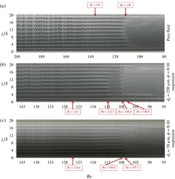
Space–time diagrams for (a) pure fluid, (b)
 $\unicode[STIX]{x1D719}=0.10$
suspension of
 $d_{p}\approx 230~\unicode[STIX]{x03BC}\text{m}$
particles, and (c)
 $\unicode[STIX]{x1D719}=0.10$
suspension of
 $d_{p}\approx 70~\unicode[STIX]{x03BC}\text{m}$
particles, each constructed from images taken at an interval of 50 s between frames from decreasing-
 $Re$
experiments with
 $\text{d}Re/\text{d}\unicode[STIX]{x1D70F}=-0.0031$
. The
 $Re$
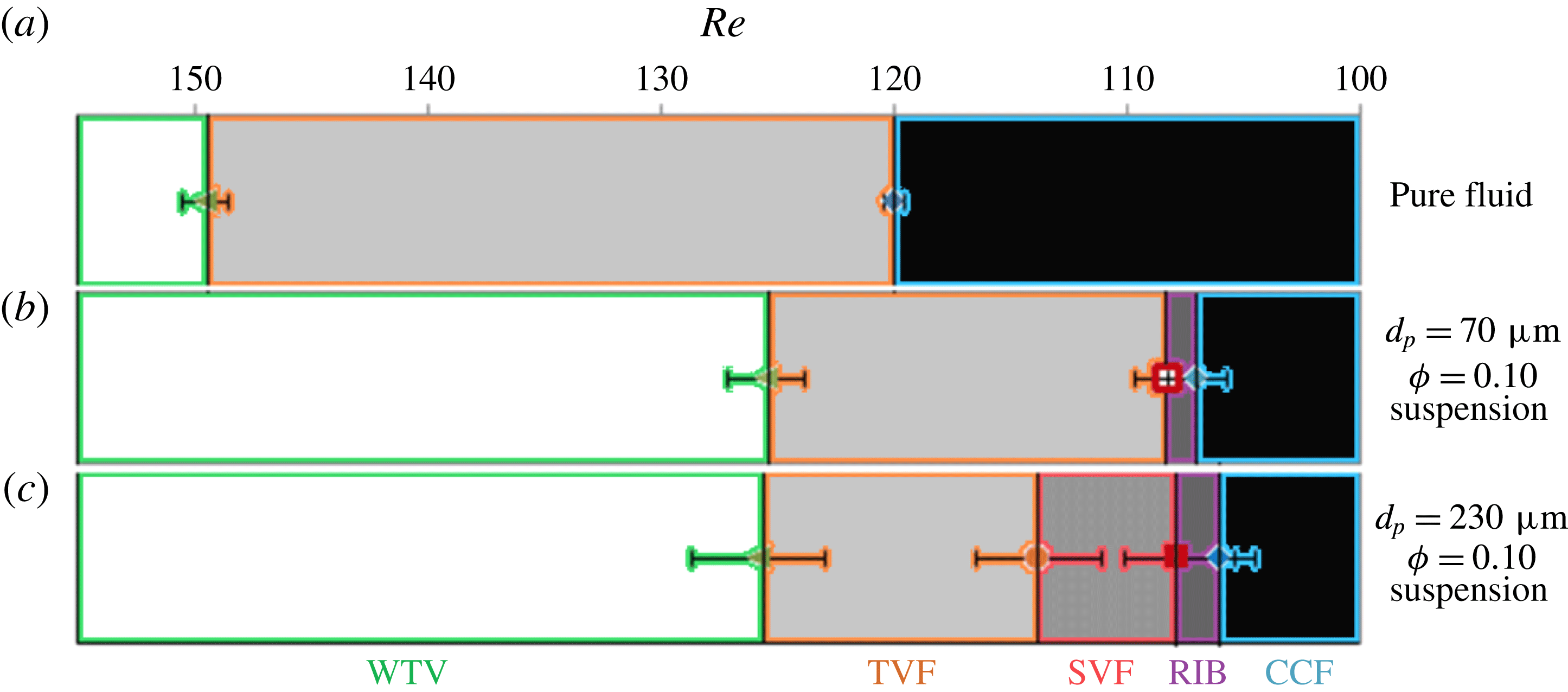
values corresponding to flow transitions are labelled. The flow transition sequence is from WTV to TVF to CCF for the pure fluid while for
 $\unicode[STIX]{x1D719}=0.10$
suspensions, the sequence is from WTV to TVF to non-axisymmetric states (spirals and ribbons) to CCF. Flow transitions took place at lower
 $Re$
for the suspensions compared to the pure fluid, while reduction of particle size reduced the range of
 $Re$
over which the non-axisymmetric flow states are seen.

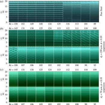
Space–time diagrams at various
 $Re$
for (a) pure fluid, (b)
 $\unicode[STIX]{x1D719}=0.10$
suspension of
 $d_{p}\approx 230~\unicode[STIX]{x03BC}\text{m}$
particles, and (c)
 $\unicode[STIX]{x1D719}=0.10$
suspension of
 $d_{p}\approx 70~\unicode[STIX]{x03BC}\text{m}$
particles, each constructed from images taken at
 $60~\text{frames}~\text{s}^{-1}$
from a decreasing-
 $Re$
experiment with
 $\text{d}Re/\text{d}\unicode[STIX]{x1D70F}=-0.0031$
. The diagram for each
 $Re$
represents a time duration of 3.8 s for pure fluid and 4 s for the suspensions. The flow transitions were from WTV to TVF to CCF for the pure fluid. For
 $\unicode[STIX]{x1D719}=0.10$
suspension of
 $230~\unicode[STIX]{x03BC}\text{m}$
particles, additional spiral vortex flow and ribbons appeared between TVF and CCF. For
 $\unicode[STIX]{x1D719}=0.10$
suspension, when the particle size is reduced to
 $d_{p}=70~\unicode[STIX]{x03BC}\text{m}$
, only the ribbon state appeared between TVF and CCF.

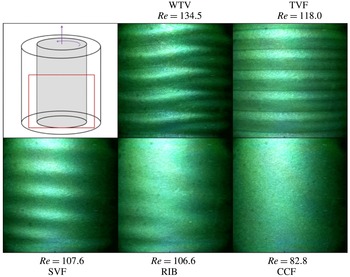
Photographs of flow structures for
 $\unicode[STIX]{x1D719}=0.10$
suspension of
 $d_{p}\approx 230~\unicode[STIX]{x03BC}\text{m}$
particles observed during a decreasing-
 $Re$
ramp with
 $\text{d}Re/\text{d}\unicode[STIX]{x1D70F}=-0.0031$
. The red rectangle in the top left section shows the area photographed for this figure. WTV and TVF states can be seen at
 $Re=134.5$
and
 $Re=118$
, respectively. Spirals merging into the bottom Ekman layer can be seen in the SVF at
 $Re=107.6$
, as in the space–time diagrams for
 $112\geqslant Re\geqslant 109$
in figure 7(b). The RIB state at
 $Re=110$
shows the azimuthal location where upward rotating vortices change into downward rotating vortices and vice versa at the same axial height (also seen in the space–time diagram for
 $Re=108$
in figure 7(b)).

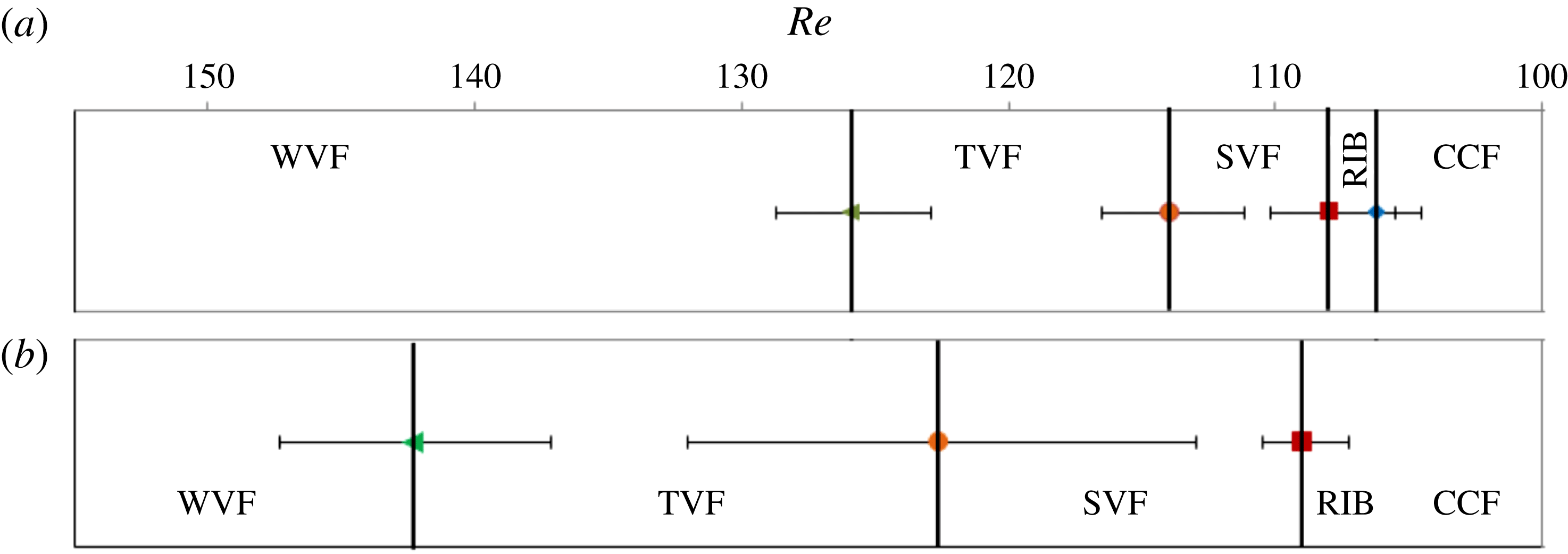
Compilation of
 $Re$
corresponding to various flow structures and transitions for (a) pure fluid, and suspensions at
 $\unicode[STIX]{x1D719}=0.10$
for particles of size (b)
 $d_{p}\approx 70~\unicode[STIX]{x03BC}\text{m}$
particles, and (c)
 $d_{p}\approx 230~\unicode[STIX]{x03BC}\text{m}$
particles. Each case displays the average of seven decreasing-
 $Re$
ramp experiments at
 $\text{d}Re/\text{d}\unicode[STIX]{x1D70F}=-0.0031$
. Error bars show the standard deviation from the average transition
 $Re$
. Non-axisymmetric flow structures (SVF, RIB) appear for the suspensions which do not appear for pure fluid. SVF and RIB appeared for the suspension of
 $d_{p}\approx 230~\unicode[STIX]{x03BC}\text{m}$
, while only RIB appeared for
 $d_{p}\approx 70~\unicode[STIX]{x03BC}\text{m}$
.

Figure 6 shows the space–time diagrams constructed from photographs recorded at intervals of 50 s for three cases: (a) pure fluid for
 $209\geqslant Re\geqslant 89$
, (b)
 $\unicode[STIX]{x1D719}=0.10$
suspension of
 $d_{p}\approx 230~\unicode[STIX]{x03BC}\text{m}$
particles for
 $145\geqslant Re\geqslant 93$
, and (c)
 $\unicode[STIX]{x1D719}=0.10$
suspension of
 $d_{p}\approx 70~\unicode[STIX]{x03BC}\text{m}$
particles for
 $145\geqslant Re\geqslant 93$
. In the range of
 $Re$
studied, the flow transition sequence was from WTV to TVF to CCF for the pure fluid. By contrast, for the
 $\unicode[STIX]{x1D719}=0.10$
suspension of
 $d_{p}\approx 230~\unicode[STIX]{x03BC}\text{m}$
particles, the flow transitions were from WTV to TVF to non-axisymmetric flow states (spirals and ribbons, as described below) to CCF. When the particle size was reduced to
 $d_{p}\approx 70~\unicode[STIX]{x03BC}\text{m}$
, the suspension followed the same sequence of flow transitions as those for the
 $d_{p}\approx 230~\unicode[STIX]{x03BC}\text{m}$
particle suspension, but the
 $Re$
range corresponding to the non-axisymmetric flow states was reduced.
Figure 7 shows space–time diagrams constructed from 3–4 s durations of
 $60~\text{frames}~\text{s}^{-1}$
images for (a) pure fluid, (b)
 $\unicode[STIX]{x1D719}=0.10$
suspension of
 $d_{p}\approx 230~\unicode[STIX]{x03BC}\text{m}$
particles, and (c)
 $\unicode[STIX]{x1D719}=0.10$
suspension of
 $d_{p}\approx 70~\unicode[STIX]{x03BC}\text{m}$
particles. For the
 $\unicode[STIX]{x1D719}=0.10$
suspension of
 $d_{p}\approx 230~\unicode[STIX]{x03BC}\text{m}$
particles, space–time diagrams at
 $Re=145,131,130$
and
 $125$
show counter-rotating pairs of wavy Taylor vortices (WTV) with larger azimuthal wavelength at smaller
 $Re$
. Between
 $Re=125$
and
 $Re=124$
, a transition from WTV into Taylor vortex flow (TVF) is observed. Space–time diagrams at
 $Re=124$
and
 $113$
show axisymmetric counter-rotating pairs of Taylor vortices filling the full annulus length; note that non-CCF states persist to lower
 $Re$
than seen for the pure fluid.
In addition to the reduced
 $Re$
for the transition back to CCF, between
 $Re=113$
and
 $Re=112$
, axisymmetry is lost as the TVF breaks down to form spiral vortex flow (SVF). The space–time diagram at
 $Re=112$
shows spiral structure in the middle section of the annulus with a pair of counter-rotating vortices spiralling around the inner cylinder merging into Taylor vortices at top and bottom. The merging location of spirals and Taylor vortices creates defects and disturbs the axisymmetry of these Taylor vortices, resulting in their azimuthal waviness. Between
 $Re=109$
and
 $Re=108$
, the spirals give way to another non-axisymmetric flow structure called ribbons (RIB), in which pairs of time-modulated counter-rotating vortices fill the annular length. The two counter-rotating vortices in each pair alternate in time between upward and downward rotation (as seen at the outer wall). The space–time diagram for the RIB state can be seen in figure 7(b). Between
 $Re=108$
and
 $Re=106$
, the flow transitioned from ribbons into CCF.
Figure 8 shows photographs of flow structures for
 $\unicode[STIX]{x1D719}=0.10$
and
 $d_{p}\approx 230~\unicode[STIX]{x03BC}\text{m}$
: the flow states observed are WTV at
 $Re=134.5$
, TVF at
 $Re=118$
, SVF at
 $Re=107.6$
, RIB at
 $Re=106.6$
and CCF at
 $Re=82.8$
. The spirals shown in figures 7 and 8 appear to translate upwards in the laboratory frame of reference, but in other experiments with the same parameters, spirals translating downwards were observed indicating symmetry with respect to this flow state. For the smaller particles of
 $d_{p}\approx 70~\unicode[STIX]{x03BC}\text{m}$
, the space–time diagrams in figure 7 show the flow transition with decreasing
 $Re$
from WTV to TVF to RIB to CCF without appearance of SVF.
The
 $Re$
ramp down experiments for pure fluid, as well as suspensions at
 $\unicode[STIX]{x1D719}=0.10$
for both
 $d_{p}\approx 230~\unicode[STIX]{x03BC}\text{m}$
and
 $d_{p}\approx 70~\unicode[STIX]{x03BC}\text{m}$
particles, described above were repeated seven times for each material. In two of the seven experiments, we started at
 $Re$
corresponding to WVF and then ramped down the rotation rate until CCF was observed. In the other five experiments we started at
 $Re$
corresponding to TVF and ramped down to CCF. In figure 9,
 $Re$
corresponding to various flow transitions are compiled with error bars showing the standard deviation from the average value of transition
 $Re$
; figure 7 shows space–time diagrams of the flow structures. The first primary difference between the pure fluid and suspension is that the boundary between WTV and TVF for
 $\unicode[STIX]{x1D719}=0.10$
and
 $d_{p}=230~\unicode[STIX]{x03BC}\text{m}$
was observed at smaller
 $Re$
than for pure fluid. The pure fluid went through a transition from axisymmetric TVF to axisymmetric CCF. By contrast, an even more striking deviation from the pure fluid behaviour was seen for the suspension in an interval of
 $113\geqslant Re\geqslant 107$
, as stable non-axisymmetric flow structures (SVF and RIB) appeared between the axisymmetric TVF and CCF. The transition into CCF for
 $\unicode[STIX]{x1D719}=0.10$
and
 $d_{p}\approx 230~\unicode[STIX]{x03BC}\text{m}$
is at
 $Re=107$
, well below the
 $Re=120$
found for this transition in the pure fluid. For the smaller particle size of
 $d_{p}\approx 70~\unicode[STIX]{x03BC}\text{m}$
, the non-axisymmetric region consisted only of RIB, as SVF did not appear. As a final point, the range of
 $Re$
for this region reduced to
 $107.8\geqslant Re\geqslant 106.8$
, but reduction of the particle size did not noticeably change the
 $Re$
corresponding to transitions of WVF to TVF, into RIB or from RIB to CCF.
Compilation of
 $Re$
corresponding to various flow structures and transitions for
 $\unicode[STIX]{x1D719}=0.10$
suspension with particles of size
 $d_{p}\approx 230~\unicode[STIX]{x03BC}\text{m}$
during (a) decreasing-
 $Re$
ramp, and (b) increasing-
 $Re$
ramp. Various flow transitions were found to occur at higher
 $Re$
during the increasing-
 $Re$
ramp compared to during the decreasing-
 $Re$
ramp showing significant hysteresis. Note that in figure (b) the CCF–RIB transition is not captured as in these experiments we started with the
 $Re$
in the RIB region and increased
 $Re$
.

Space–time diagram constructed from images recorded at
 $60~\text{frames}~\text{s}^{-1}$
during decreasing-
 $Re$
ramp with
 $\text{d}Re/\text{d}\unicode[STIX]{x1D70F}=-0.0031$
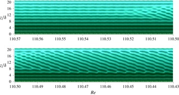
. The TVF–SVF transition for
 $\unicode[STIX]{x1D719}=0.10$
suspension of
 $d_{p}\approx 230~\unicode[STIX]{x03BC}\text{m}$
particles occurs in the range
 $110.57\geqslant Re\geqslant 110.43$
.

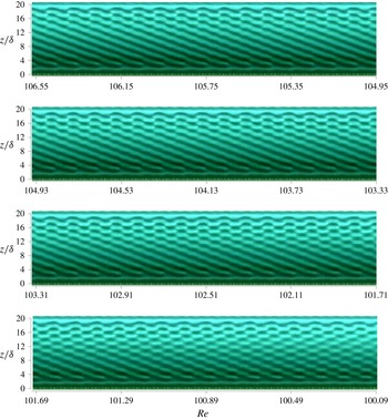
Space–time diagram constructed from images recorded at
 $60~\text{frames}~\text{s}^{-1}$
during decreasing-
 $Re$
ramp with
 $\text{d}Re/\text{d}\unicode[STIX]{x1D70F}=-0.0031$
. The SVF–RIB transition for
 $\unicode[STIX]{x1D719}=0.10$
suspension of
 $d_{p}\approx 230~\unicode[STIX]{x03BC}\text{m}$
particles occurs gradually in the range
 $106.57\geqslant Re\geqslant 100.09$
.

Space–time diagram constructed from images recorded at
 $60~\text{frames}~\text{s}^{-1}$
during decreasing-
 $Re$
ramp with
 $\text{d}Re/\text{d}\unicode[STIX]{x1D70F}=-0.0031$
. The TVF–RIB transition for
 $\unicode[STIX]{x1D719}=0.10$
suspension of
 $d_{p}\approx 70~\unicode[STIX]{x03BC}\text{m}$
particles occurs in the range
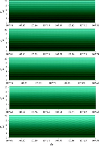
 $107.88\geqslant Re\geqslant 107.54$
.

Space–time diagram constructed from images recorded at
 $60~\text{frames}~\text{s}^{-1}$
during decreasing-
 $Re$
ramp with
 $\text{d}Re/\text{d}\unicode[STIX]{x1D70F}=-0.0031$
. The RIB–CCF transition for
 $\unicode[STIX]{x1D719}=0.10$
suspension of
 $d_{p}\approx 70~\unicode[STIX]{x03BC}\text{m}$
particles occurs in the range
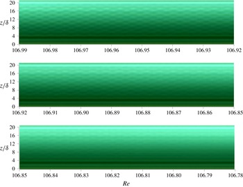
 $106.99\geqslant Re\geqslant 106.78$
.

Additional experiments were performed with
 $\unicode[STIX]{x1D719}=0.1$
suspension with particles of size
 $d_{p}\approx 230~\unicode[STIX]{x03BC}\text{m}$
to study the hysteresis in flow transitions. Starting with a value of
 $Re$
in the TVF regime,
 $Re$
is reduced slowly until RIB is reached and ramped up slowly to a
 $Re$
corresponding to WVF. The flow transitions and flow structures during a decreasing-
 $Re$
ramp experiment are compared against those during an increasing-
 $Re$
ramp in figure 10. Note that the CCF–RIB transition for the increasing-
 $Re$
was not captured as we started from a
 $Re$
that is above this transition. The flow transitions in both cases are observed to be qualitatively the same but quantitatively different. All the flow transitions during the increasing-
 $Re$
ramp were observed to occur at higher
 $Re$
compared to during decreasing-
 $Re$
ramp experiments showing significant hysteresis. Recall that the pure fluid showed no hysteresis with respect to the direction of ramp rate.
3.3.2 Flow transitions
The TVF to SVF transition for the
 $\unicode[STIX]{x1D719}=0.10$
suspension of
 $d_{p}\approx 230~\unicode[STIX]{x03BC}\text{m}$
particles during a decreasing-
 $Re$
ramp experiment with
 $\text{d}Re/\text{d}\unicode[STIX]{x1D70F}=-0.0031$
is shown in the space–time diagram of figure 11. As
 $Re$
decreased, the pair of vortices in the middle section of TVF became unstable and the flow quickly adjusted to form spiral vortices, with a region of Taylor vortices above and below. With further reduction in
 $Re$
, the spirals expanded into the remaining Taylor vortices until the annular length was fully SVF, except for the top and bottom Ekman rolls.
The SVF to RIB transition for
 $\unicode[STIX]{x1D719}=0.10$
and
 $d_{p}\approx 230~\unicode[STIX]{x03BC}\text{m}$
during a decreasing-
 $Re$
ramp experiment at
 $\text{d}Re/\text{d}\unicode[STIX]{x1D70F}=-0.0031$
is shown in the space–time diagram in figure 12. With the reduction of
 $Re$
, spiral vortices in the top section of the SVF flow became unstable and broke into ribbons. This unstable section, with reduction in
 $Re$
, gradually expanded towards the bottom portion of the annulus until the full length was RIB, with top and bottom Ekman rolls.
The TVF to RIB transition at
 $\unicode[STIX]{x1D719}=0.10$
for the smaller
 $d_{p}\approx 70~\unicode[STIX]{x03BC}\text{m}$
particles during a decreasing-
 $Re$
ramp at
 $\text{d}Re/\text{d}\unicode[STIX]{x1D70F}=-0.0031$
is shown in figure 13. With reduction of
 $Re$
, the Taylor vortices in the middle section of the annulus length became unstable and initially turned into CCF. This region quickly expanded into the top and bottom Taylor vortices. A slowly developing instability appeared in this CCF to form spatially irregular ribbons which eventually organized into ribbons (RIB). This transition differed from the SVF to RIB transition, as it was slow to establish the RIB structure.
The RIB to CCF transition for
 $\unicode[STIX]{x1D719}=0.10$
and
 $d_{p}\approx 70~\unicode[STIX]{x03BC}\text{m}$
at
 $\text{d}Re/\text{d}\unicode[STIX]{x1D70F}=-0.0031$
is shown in figure 14. With reduction of
 $Re$
, the ribbons in the middle section of the annulus disappeared over a small
 $Re$
range leaving CCF with top and bottom Ekman rolls.
3.3.3 Transient evolution
Experiments to examine the transient evolution of suspension flow at fixed
 $Re$
over extended periods of time (rather than slowly ramped as described previously) were performed. These experiments only considered the single concentration of
 $\unicode[STIX]{x1D719}=0.10$
with both particle sizes,
 $d_{p}\approx 70~\unicode[STIX]{x03BC}\text{m}$
and
 $d_{p}\approx 230~\unicode[STIX]{x03BC}\text{m}$
. This provides information on system dynamics distinct from and complementary to the quasi-steady evolution probed with a slowly ramped rotation rate. First, the inner cylinder was rotated at
 $Re=165.6$
to establish WTV and held for 120 s for particle mixing. The inner cylinder was then stopped and held stationary for 120 s to ensure no residual flow. The inner cylinder was then rotated at
 $Re=99.3$
for 120 s to establish CCF, after which
 $Re$
was raised as rapidly as possible to a given fixed
 $Re$
. The flow evolution with time at this latter
 $Re$
was recorded over
 $30$
min, during which time the flow was photographed at regular intervals for a duration of 3 s at a rate of
 $60~\text{frames}~\text{s}^{-1}$
. The resulting images were used to construct space–time diagrams. The procedure was repeated for several
 $Re$
in the ranges
 $105.5\leqslant Re\leqslant 110.7$
for
 $d_{p}\approx 70~\unicode[STIX]{x03BC}\text{m}$
and
 $101.4\leqslant Re\leqslant 119.0$
for
 $d_{p}\approx 230~\unicode[STIX]{x03BC}\text{m}$
. Note that the diffusion time scale here is
 $t_{d}\approx 1.5~\text{s}$
, far shorter than the 1800 s duration of each of these experiments.
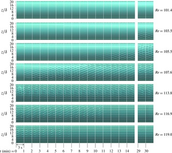
Transient evolution experiments. Space–time diagrams for a suspension of
 $\unicode[STIX]{x1D719}=0.10$
and
 $d_{p}\approx 230~\unicode[STIX]{x03BC}\text{m}$
when the
 $Re$
is rapidly increased from
 $Re=99.3$
(CCF) to a higher value (shown on the right) and held constant for 1800 s (30.0 min). The diagrams are constructed from images taken at a rate of
 $60~\text{frames}~\text{s}^{-1}$
. The diagram at each
 $Re$
in the range
 $101.4\leqslant Re\leqslant 119.0$
is a compilation of space–time slices each 3 s in duration separated by 60 s. The flow structures are CCF at
 $Re=101.4$
, partial RIB at
 $Re=103.5$
, RIB at
 $Re=105.5$
, SVF at
 $Re=107.6$
and
 $Re=113.8$
, and TVF at
 $Re=116.9$
and
 $Re=119.0$
.

The space–time diagrams at various
 $Re$
for the suspension of
 $d_{p}\approx 230~\unicode[STIX]{x03BC}\text{m}$
are shown in figure 15. At each
 $Re$
, the space–time diagrams of 3 s duration are separated by
 $1$
min. The space–time diagrams for
 $0\leqslant t\leqslant 14$
min show the evolution of the flow structures with time and the diagrams at
 $t=29$
and
 $30$
min show the fully developed flow structures at the end of the experiment. At
 $Re=101.4$
, which is below the TVF–CCF transition
 $Re$
, the flow rapidly formed CCF in the full length of the annulus with the exception of top and bottom Ekman layers, and this structure was retained for the remainder of the experiment. At
 $Re=105.5$
, the initial CCF slowly became unstable and took
 $13$
min to form ribbon structures (RIB) in the full annular length. The fully developed RIB was seen at the end of the
 $30$
min duration of the experiment. At
 $Re=103.5$
, the flow was CCF for most of the time, but towards the end RIB structures appeared in the bottom half of the annular section. At
 $Re=107.6$
and
 $113.8$
, the flow became unstable in short time and evolved from CCF to RIB and finally into a combination of spirals and Taylor vortices with azimuthal waviness that remained to the end of the run. At
 $Re=116.9$
and
 $119$
, the flow in the annulus became unstable immediately to form a combination of spirals and Taylor vortices in the full length, eventually evolving to the final state of TVF.
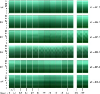
Space–time diagrams showing the time evolution of flow structures for the suspension of
 $d_{p}\approx 70~\unicode[STIX]{x03BC}\text{m}$
are shown in figure 16. The diagram at each
 $Re$
between
 $Re=105.5$
and
 $Re=110.7$
is a compilation of space–time slices of 3 s, separated by 30 s. The space–time diagrams between
 $0\leqslant t\leqslant 5.0$
min show the evolution of the flow structures with time and the diagrams at
 $t=29.5$
and
 $30.0$
min show the fully developed flow structures. At
 $Re=105.5$
and
 $Re=106.6$
the flow quickly established CCF with Ekman layers at top and bottom. At
 $Re=107.6$
, the flow slowly became unstable to form a regular RIB structure after
 $5$
min and this remained unchanged to 30 min. At
 $Re=108.6$
, TVF was established quickly in the bottom part and the fluid between this region and top Ekman layer became unstable to form RIB after
 $1.5$
min. This partial TVF–RIB structure persisted to 30 min. Finally, at
 $Re=109.7$
and
 $Re=110.7$
, the flow quickly established TVF, which persisted until
 $30$
min.
Transient evolution experiments. Space–time diagrams for a suspension of
 $\unicode[STIX]{x1D719}=0.10$
and
 $d_{p}\approx 70~\unicode[STIX]{x03BC}\text{m}$
when
 $Re$
is rapidly increased from
 $Re=99.3$
(CCF) to a specific value and kept constant for 1800 s (30 min). The diagrams are constructed from images taken at a rate of
 $60~\text{frames}~\text{s}^{-1}$
. The diagram at each
 $Re$
in the range
 $105.5\leqslant Re\leqslant 110.7$
is a compilation of space–time slices each 3 s in duration separated by 30 s. The flow structures are CCF at
 $Re=105.5$
and
 $Re=106.6$
, RIB at
 $Re=107.6$
and
 $Re=108.6$
, and TVF at
 $Re=109.7$
and
 $Re=110.7$
.

Photographs of (a) spiral vortex flow (SVF) at
 $Re=107.6$
, and (b) ribbons (RIB) at
 $Re=106.6$
for a suspension of
 $\unicode[STIX]{x1D719}=0.10$
and
 $d_{p}\approx 230~\unicode[STIX]{x03BC}\text{m}$
particles at various times (
 $t$
) during two rotations of the inner cylinder. Here
 $T$
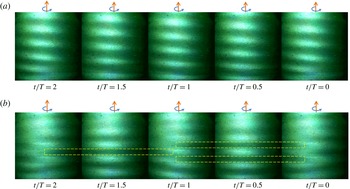
is the time for the inner cylinder to complete one full rotation. Both SVF and RIB complete one full cycle in two inner cylinder rotations indicating an azimuthal wave speed that is half of the inner cylinder rotation speed. One pair of vortices in SVF originating at the bottom shift axially by one pair width (2
 $\unicode[STIX]{x1D6FF}$
) in one rotation around the inner cylinder (
 $\unicode[STIX]{x1D703}=2\unicode[STIX]{x03C0}$
). The RIB cycle here has half-downward rotating (dark region marked with dashed yellow rectangles) and half-upward rotating (bright region) vortices with rotation direction described as seen at the outer wall.

Space–time diagrams for (a) spiral vortex flow (SVF) at
 $Re=107.6$
, and (b) ribbons (RIB) at
 $Re=106.6$
for a suspension of
 $\unicode[STIX]{x1D719}=0.10$
and
 $d_{p}\approx 230~\unicode[STIX]{x03BC}\text{m}$
particles during eight rotations of the inner cylinder. Here,
 $T$
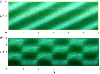
is the time for the inner cylinder to complete one full rotation. SVF and RIB completed one full cycle in two inner cylinder rotations indicating an azimuthal wave speed that is half of the inner cylinder rotation rate. One pair of vortices in SVF originating at the bottom shift one vortex pair width (2
 $\unicode[STIX]{x1D6FF}$
) in the axial direction during one rotation around the inner cylinder. The RIB cycle here has half-downward rotating (dark region) and half-upward rotating (bright region) vortices around the inner cylinder.

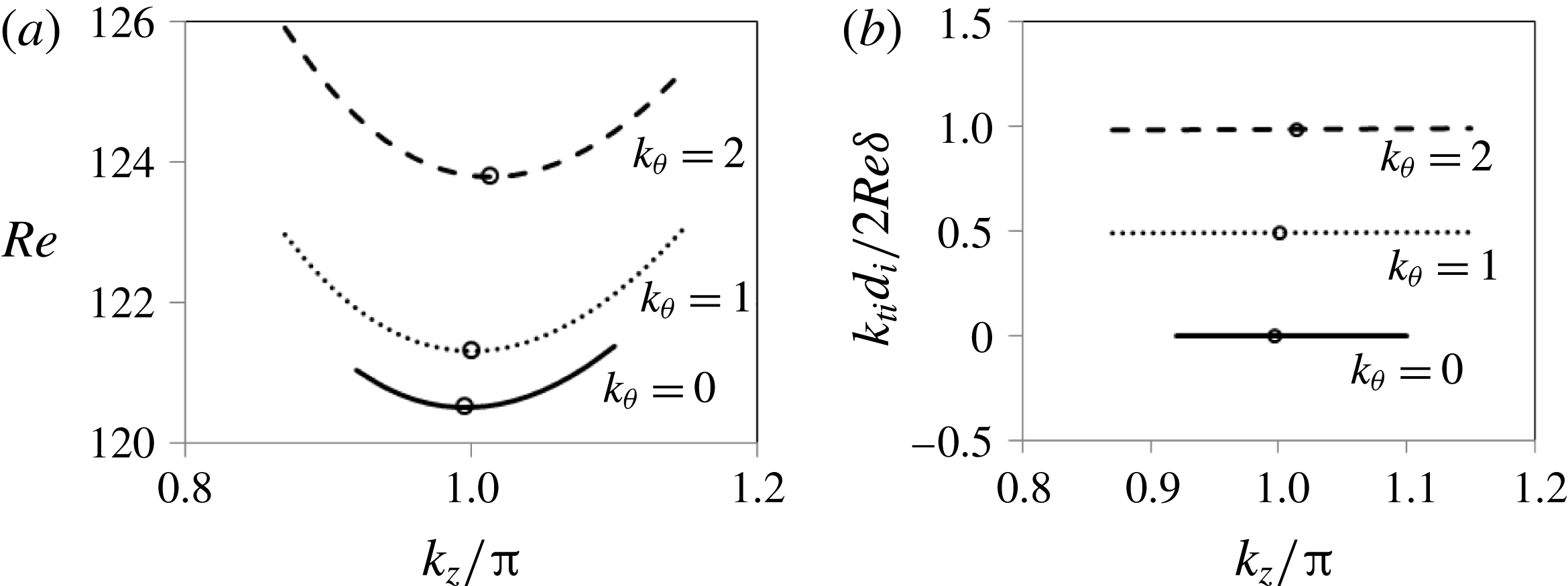
Marginal stability curves from linear stability analysis for the pure fluid sheared between the rotating inner cylinder and stationary outer cylinder. Here,
 $k_{\unicode[STIX]{x1D703}}=0,1$
and
 $2$
represent Taylor vortex flow (TVF), mode 1 spiral vortex flow (SVF) and mode 2 SVF structures. Circles in (a) indicate the minimum
 $Re$
on each marginal stability curve. The lowest
 $Re$
on the curves is
 $Re=120.5$
at
 $k_{\unicode[STIX]{x1D703}}=0$
and
 $k_{z}/2\unicode[STIX]{x03C0}=0.996$
which corresponds to TVF. The vertical axis in (b) represents the ratio of azimuthal wave speed for the flow structure to the inner cylinder rotation rate, e.g. the mode 1 spiral has an azimuthal wave speed that is half that of the inner cylinder rotation. The circles correspond to the minimum
 $Re$
on each curve.

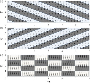
Space–time diagrams of (a) L-spiral (mode -1), (b) R-spiral (mode 1), and (c) ribbons constructed from velocity fields computed using linear stability analysis for the pure fluid with rotating inner cylinder and stationary outer cylinder. The ribbon structure is created by superimposing an L- and an R-spiral. Shown are the velocity vectors in the
 $z$
–
 $t$
plane at
 $\unicode[STIX]{x1D703}=0$
and
 $r=d_{i}/2+0.8\unicode[STIX]{x1D6FF}$
, where
 $d_{i}$
is the inner cylinder diameter and
 $\unicode[STIX]{x1D6FF}$
is the annular gap;
 $T$
is the time for the inner cylinder to complete one full rotation. The space–time diagrams for the R-spiral and ribbon structures here are the same as those for the SVF and RIB in figure 18 in terms of wavelengths and wave speeds.

The final flow structures at fixed
 $Re$
observed at the end of the
 $30$
min of these experiments were the same as those determined from the quasi-steady experiments with slow ramping of
 $Re$
as shown in figure 9. The conclusion we draw is that the ultimate states are relatively independent of the path to them for all of these conditions. The flow for the suspension with
 $d_{p}\approx 70~\unicode[STIX]{x03BC}\text{m}$
particles took less time to evolve into fully developed structures than for the suspension with
 $d_{p}\approx 230~\unicode[STIX]{x03BC}\text{m}$
particles. This leads to the same conclusion drawn from the quasi-steady experiments, namely that the reduction of the particle size leads to a behaviour closer to that of the pure fluid.
3.4 Characterization of spiral and ribbon structures
Photographs and space–time diagrams of spiral and ribbon structures during two rotations of the inner cylinder are displayed in figures 17 and 18. In the case of spirals at
 $Re=107.6$
, an axial length of two times the annular gap (
 $2\unicode[STIX]{x1D6FF}$
) was found for a pair of counter-rotating vortices (downward rotating and upward rotating at the outer wall are seen as darker and brighter regions, respectively, in these figures). The vortex pair was observed to shift by
 $2\unicode[STIX]{x1D6FF}$
in the axial direction while it completed one rotation, or
 $\unicode[STIX]{x0394}\unicode[STIX]{x1D703}=2\unicode[STIX]{x03C0}$
, around the inner cylinder, indicating mode 1 spiral structure (various modes of the spiral structures are discussed in the later part of this section in connection with linear stability theory). The spiral completed one cycle in the azimuthal direction in the time the inner cylinder took to complete two rotations, i.e. the azimuthal spiral wave speed is half that of the inner cylinder.
For ribbons at
 $Re=106.6$
, the axial width of each vortex structure was observed to be the same as the annular gap (
 $\unicode[STIX]{x1D6FF}$
). The structures in the azimuthal direction consist of half (
 $\unicode[STIX]{x0394}\unicode[STIX]{x1D703}=\unicode[STIX]{x03C0}$
) downward rotating vortex (marked with dashed yellow rectangle) and half (
 $\unicode[STIX]{x0394}\unicode[STIX]{x1D703}=\unicode[STIX]{x03C0}$
) upward rotating vortex (with rotation directions seen at the outer wall). At the two azimuthal locations where these two vortices meet, cancelation of vorticities resulted in circular Couette flow. This vortex around the inner cylinder completed one cycle in two inner cylinder rotations indicating an azimuthal wave speed that is half of the inner cylinder rotation speed. This ribbon structure can be obtained by superposition of two mode 1 spirals, one spiralling clockwise and the other in the counter-clockwise sense when seen from the top view.
We sought a quantitative comparison of the spiral and ribbon structures described above for the suspension with those obtained for pure fluid. For this purpose, we have used linear stability analysis (LSA). The primary question to be answered is whether the observed wavelengths and wave speeds of the structures in the suspension agree with those predicted by LSA for the pure fluid with only the inner cylinder rotating; note these are not structures accessed by the pure fluid, and differ from those seen with both inner and outer cylinder moving with counter-rotation. The circular Couette base flow has only azimuthal component
 $U_{\unicode[STIX]{x1D703}}(r)$
which for a Newtonian fluid with rotating inner cylinder and stationary outer cylinder in cylindrical coordinates (
 $r,\unicode[STIX]{x1D703}$
and
 $z$
denoting radial, azimuthal and axial coordinates, respectively) is given by
 $$\begin{eqnarray}U_{\unicode[STIX]{x1D703}}(r)=Ar+Br^{-1};\quad A=\frac{-d_{i}^{2}\unicode[STIX]{x1D6FA}}{d_{o}^{2}-d_{i}^{2}};\quad B=\frac{d_{o}^{2}d_{i}^{2}\unicode[STIX]{x1D6FA}}{d_{o}^{2}-d_{i}^{2}}.\end{eqnarray}$$
This flow generates a centrifugal acceleration which is balanced by the pressure field. In the standard fashion, a perturbation of the base flow and pressure fields by
 $\boldsymbol{u}^{\prime }=(u_{r}^{\prime },u_{\unicode[STIX]{x1D703}}^{\prime },u_{z}^{\prime })$
,
 $p^{\prime }$
is summed with the base flow and the resulting velocity and pressure fields are inserted to the Navier–Stokes equations, with neglect of nonlinear terms in perturbed quantities. It should be noted that values of the perturbed field are zero at the inner and outer cylinder walls. Details are shown in appendix A. We provide only results of primary interest to the current study.
The marginal stability curves determined from the analysis shown in figure 19 indicate the relations between
 ${k_{t}}_{i},k_{\unicode[STIX]{x1D703}}$
and
 $k_{z}$
which are the wavenumbers in time, azimuthal and axial directions. Here
 $k_{\unicode[STIX]{x1D703}}=0,1$
and
 $2$
represent TVF, mode 1 spiral and mode 2 spiral, respectively. For pure fluid, the first non-CCF state which is physically realized as
 $Re$
increases corresponds to the minimum
 $Re$
point on the lowest marginal stability curve, which is at the parameter values
 $k_{\unicode[STIX]{x1D703}}=0$
,
 $Re=120.5$
,
 $k_{z}/\unicode[STIX]{x03C0}=0.996$
and
 $k_{ti}=0$
: this is Taylor vortex flow. For flow driven by a rotating inner cylinder and stationary outer cylinder, the spiral vortex flow solution is not realized for the pure fluid. However, we can compare the analytical predictions of the two (left L, and right R) spiral structures to our observations for the suspension. The L-spiral has parameters
 $k_{\unicode[STIX]{x1D703}}=-1$
,
 $Re=121.303$
,
 $k_{z}/\unicode[STIX]{x03C0}=1.0008$
and
 $k_{ti}=-8.1353$
and the R-spiral has
 $k_{\unicode[STIX]{x1D703}}=1$
,
 $Re=121.303$
,
 $k_{z}/\unicode[STIX]{x03C0}=1.0008$
and
 $k_{ti}=8.1353$
. The variation in time of the velocity vectors of the L- and R-spirals along a line (
 $r=d_{i}/2+0.8\unicode[STIX]{x1D6FF}$
,
 $\unicode[STIX]{x1D703}=0$
,
 $z$
) is shown in the space–time diagrams of figure 20(a,b). The space–time diagram for ribbons in figure 20(c) is constructed from superimposing R- and L-spirals. The space–time diagrams for the R-spiral and ribbon structures reveal that the azimuthal wave speed is half of the inner cylinder rotation speed and the axial wavelength is the same as the annular gap,
 $\unicode[STIX]{x1D6FF}$
. These results agree with the wave speed and wavelength of spirals and ribbons observed in the suspension flow (see figure 18). From this, we conclude that the suspension is apparently accessing the spiral and ribbon structures that satisfy the pure fluid problem, rather than distinct flow structures.
The experiments with the suspensions showed that the flow structures at a given
 $Re$
are the same for both cases: the quasi-steady ramp rate (§ 3.3.1) and instant rise of
 $Re$
from CCF (§ 3.3.3). This indicates that the inertially migrated concentration profiles are not the reason for accessing spirals and ribbons. Note that the radial concentration profiles in the spirals and ribbons are uniform as the time scale of the transient modulation of these structures is much smaller compared to the time scale of inertial migration. Furthermore, the linear stability analysis of circular Couette flow of a fluid with inertially migrated concentration profiles showed that these radially varying profiles neither produce spirals and ribbons after instability nor the instability at lower
 $Re$
compared to the pure fluid. The details of the analysis are described in the supplementary material available at https://doi.org/10.1017/jfm.2017.754 attached to this paper, and the key points are given below.
An additional linear stability analysis of the circular Couette flow is performed for a fluid with radially varying viscosity profile in the annular region to take into account the concentration variation due to inertial migration. Three profiles of radially varying relative viscosity,
 $f(r)$
, corresponding to the three concentration profiles, are considered. Two centre peaking concentration profiles for
 $\unicode[STIX]{x1D719}_{avg}=0.025$
and 0.1, to simulate the steady concentration profiles taking into account the inertial migration, and one uniform concentration profile with zero concentration near the walls for
 $\unicode[STIX]{x1D719}_{avg}=0.1$
, to simulate profile corresponding to instant rise of
 $Re$
from rest to a given value, were considered. The neutral stability curves for the three cases indicate that the transition
 $Re$
for the suspension is higher than that of the pure fluid whereas the experiments showed otherwise. The predicted transition
 $Re$
increased with increase in
 $\unicode[STIX]{x1D719}_{avg}$
for the centre peaked profiles and reduced with increase in uniformity of the concentration profile for
 $\unicode[STIX]{x1D719}_{avg}=0.1$
. In all three cases the mode of instability is that of
 $k_{\unicode[STIX]{x1D703}}=$
0 which is Taylor vortex flow, but it is interesting and potentially significant that the wavenumber for time modulation
 $k_{ti}$
is non-zero. Note that, for a pure fluid with uniform viscosity across the annular gap, the wave speeds for
 $k_{\unicode[STIX]{x1D703}}=0$
(TVF) and
 $+/-1$
(L-SVF/R-SVF) are 0 and
 $+/-0.5$
, respectively. For the central peak
 $\unicode[STIX]{x1D719}$
profiles, the absolute value of the wave speed was observed to increase with increase in
 $\unicode[STIX]{x1D719}_{avg}$
. For
 $\unicode[STIX]{x1D719}_{avg}=0.1$
, the absolute value of the wave speed reduced towards zero with increasing uniformity of the concentration profile.
Flow state map for suspension of concentrations
 $0\leqslant \unicode[STIX]{x1D719}\leqslant 0.30$
, with
 $d_{p}\approx 230~\unicode[STIX]{x03BC}\text{m}$
. (a) Flow structures observed for suspension of
 $0\leqslant \unicode[STIX]{x1D719}\leqslant 0.30$
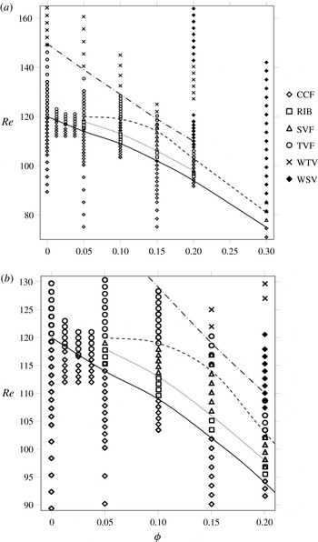
. Lines delineating various flow transitions: ——, CCF-RIB; - - - - - -, RIB-SVF; - - -, SVF-TVF; – - – - –, TVF-WTV. (b) Close-up of (a) to show the ribbon and spiral vortex regions clearly.

The results of the linear stability analysis show that a simple effective model with radially varying viscosity profiles failed to explain the experimentally observed deviations of the suspension from pure fluid in terms of the flow transition
 $Re$
and the flow structures. The analysis predicted that the modified viscosity profiles due to inertial migration stabilizes the flow whereas the experiments showed that the addition of particles destabilized the flow. We feel that a most likely candidate for the role of suspended particles is the finite-size perturbations they create in the background fluid.
3.5 Suspension experiments for
$0\leqslant \unicode[STIX]{x1D719}\leqslant 0.30$

The quasi-steady experiments, in which the
 $Re$
was slowly ramped as described in § 3.3.1, were performed for several suspension concentrations in the range
 $0\leqslant \unicode[STIX]{x1D719}\leqslant 0.30$
all for the larger particles of
 $d_{p}\approx 230~\unicode[STIX]{x03BC}\text{m}$
. A flow state diagram shown in figure 21 consolidates the various flow transitions and flow structures observed on the
 $\unicode[STIX]{x1D719}$
–
 $Re$
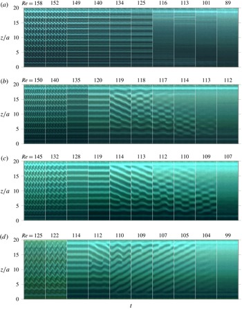
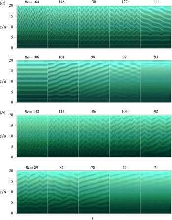
plane. Figures 22 and 23 show the space–time diagrams at different concentrations during decreasing-
 $Re$
ramp experiments, constructed from images taken at
 $60~\text{frames}~\text{s}^{-1}$
.
Space–time diagrams for suspensions of (a)
 $\unicode[STIX]{x1D719}=0$
, (b)
 $\unicode[STIX]{x1D719}=0.05$
, (c)
 $\unicode[STIX]{x1D719}=0.10$
, and (d)
 $\unicode[STIX]{x1D719}=0.15$
, all with
 $d_{p}\approx 230~\unicode[STIX]{x03BC}\text{m}$
, constructed from images taken at
 $60~\text{frames}~\text{s}^{-1}$
during decreasing-
 $Re$
experiments. The time duration for each diagram is 3.8, 3.7, 3.0 and 3.0 s for
 $\unicode[STIX]{x1D719}=0$
,
 $\unicode[STIX]{x1D719}=0.05$
,
 $\unicode[STIX]{x1D719}=0.10$
and
 $\unicode[STIX]{x1D719}=0.15$
, respectively.

Space–time diagrams for (a)
 $\unicode[STIX]{x1D719}=0.20$
, and (b)
 $\unicode[STIX]{x1D719}=0.30$
suspensions with
 $d_{p}\approx 230~\unicode[STIX]{x03BC}\text{m}$
, constructed from images taken at
 $60~\text{frames}~\text{s}^{-1}$
during decreasing-
 $Re$
experiments. The time duration for each space–time diagram is 3.7 s and 1.8 s for
 $\unicode[STIX]{x1D719}=0.20$
and
 $\unicode[STIX]{x1D719}=0.30$
, respectively.

As
 $Re$
decreased, the pure fluid transitioned from WTV to TVF to CCF as shown for
 $\unicode[STIX]{x1D719}=0$
in figure 22. For dilute suspensions with
 $0<\unicode[STIX]{x1D719}\leqslant 0.0375$
, TVF transitioned into CCF and the transition
 $Re$
was found to be decreasing with
 $\unicode[STIX]{x1D719}$
. By contrast, for
 $0.05\leqslant \unicode[STIX]{x1D719}\leqslant 0.15$
, we found that the flow transitions all follow the sequence described previously in § 3.3.1 for the
 $\unicode[STIX]{x1D719}=0.10$
suspension: as
 $Re$
was reduced, the sequence was WTV to TVF to SVF to RIB to CCF (refer to figure 22). For
 $\unicode[STIX]{x1D719}=0.20$
, an additional stable state of wavy spiral vortices (WSV) was observed at higher
 $Re$
. With reduction in
 $Re$
, the observed flows for the
 $\unicode[STIX]{x1D719}=0.20$
suspension were WSV (
 $164\geqslant Re\geqslant 141$
), WTV (
 $141\geqslant Re\geqslant 125$
), WSV (
 $125\geqslant Re\geqslant 107$
), TVF (
 $107\geqslant Re\geqslant 102$
), SVF (
 $102\geqslant Re\geqslant 96$
), RIB (
 $96\geqslant Re\geqslant 94$
) and finally CCF (
 $Re\leqslant 94$
). The WSV consists of a pair of counter-rotating vortices spiralling around the inner cylinder, similar to SVF but with waviness along the axis of the vortices. This is shown for
 $\unicode[STIX]{x1D719}=0.20$
in figure 23 for
 $Re>120$
.
With increase in the solid concentration to
 $\unicode[STIX]{x1D719}=0.30$
, WTV, TVF and RIB did not appear in the
 $Re$
range studied. As
 $Re$
decreased, the suspension at
 $\unicode[STIX]{x1D719}=0.30$
exhibited only a sequence of non-axisymmetric flow states: from WSV (
 $142\geqslant Re>82$
) to SVF (
 $82\geqslant Re>75$
) before transitioning into CCF (
 $Re\leqslant 75$
) as shown in figure 23.
The first dominant observation from the results displayed in figures 21–23 is that CCF became unstable at lower
 $Re$
with each increase in particle loading
 $\unicode[STIX]{x1D719}$
. Recall that
 $Re$
is here defined in terms of the measured effective viscosity of the bulk suspension. The second observation is that the presence of particles led to a transition in which CCF and TVF are separated by non-axisymmetric flows, including ribbons, spirals and wavy spirals. For the pure fluid with rotating inner cylinder and stationary outer cylinder, the CCF becomes unstable first to the axisymmetric TVF, and counter-rotation of the outer cylinder at
 $Re$
is required to observe non-axisymmetric SVF, as shown in figure 1.
4 Conclusions
Understanding the fluid mechanical behaviour of suspension flows requires knowledge of their flow stability. To address this issue, we have probed the inertial flow transitions of carefully density matched (neutrally buoyant) suspensions in experiments in the Taylor–Couette flow with rotating inner cylinder and stationary outer cylinder. Retaining homogeneity of the particle loading was an objective of the work, and to achieve this, the Reynolds number based on the inner cylinder rotation rate,
 $Re$
, was decreased from a well-mixed highly inertial state in a quasi-steady manner until circular Couette flow was reached. The increasing-
 $Re$
protocol, which is commonly used for studying pure fluid transitions, in which
 $Re$
is increased from CCF in a quasi-steady manner, was not used in our suspension experiments as we found it to allow a segregation of particles due to weak secondary flow in the CCF region associated with the Taylor vortices near the axial boundaries, and it was thus unsuitable for studying the uniformly mixed material.
Flow structures at various
 $Re$
and the values of
 $Re$
at flow transitions were studied for particle volume fractions
 $0<\unicode[STIX]{x1D719}\leqslant 0.30$
and compared with those observed for pure fluid (
 $\unicode[STIX]{x1D719}=0$
) in a similar decreasing-
 $Re$
experiment. To check for accumulated unsteady effects during the long-time durations of quasi-steady decreasing-
 $Re$
experiments, time evolution experiments were performed with a
 $\unicode[STIX]{x1D719}=0.10$
suspension. The inner cylinder rotation rate was increased from rest to a given
 $Re$
and the evolution of flow structures with time was observed. The one-to-one matching of long-time flow structures of the time evolution experiment with the quasi-steady decreasing-
 $Re$
experiment at corresponding
 $Re$
indicate no significant accumulated effects, i.e. the decreasing-
 $Re$
ramp corresponds to the uniform
 $\unicode[STIX]{x1D719}$
long-time results.
The quasi-steady decreasing-
 $Re$
experiments show that the pure fluid transitions from wavy Taylor vortices
 $\rightarrow$
TVF
 $\rightarrow$
CCF. In contrast to this, for suspensions with
 $d_{p}\approx 230~\unicode[STIX]{x03BC}\text{m}$
particles at
 $0.05\leqslant \unicode[STIX]{x1D719}\leqslant 0.15$
, the sequence of flow transitions followed WTV
 $\rightarrow$
TVF
 $\rightarrow$
spiral vortex flow
 $\rightarrow$
ribbons
 $\rightarrow$
CCF. The WTV transitioned into TVF just as in the pure fluid but at progressively lower
 $Re$
with increasing particle concentration. With decreasing
 $Re$
, the TVF for the suspension became unstable to non-axisymmetric disturbances resulting in transition into SVF; by contrast, the pure fluid TVF transitions to CCF. The range of
 $Re$
for which SVF was stable increased at higher particle concentration. With further decrease in
 $Re$
the SVF for a suspension gave way to another non-axisymmetric structure, ribbons, before finally becoming CCF. The
 $Re$
corresponding to SVF–RIB and RIB–CCF transitions decreased with increase in particle concentration. The appearance of the spiral and ribbon structures, which for a pure fluid appear only with both cylinders in motion with the outer counter-rotated relative to the inner, indicates that neutrally buoyant particle loading causes a qualitative alteration of the dynamical system represented by Taylor–Couette flow. Experiments with
 $\unicode[STIX]{x1D719}=0.10$
suspension showed that WVF–TVF and TVF–SVF transitions occur at higher
 $Re$
during the increasing-
 $Re$
ramp compared to during the decreasing-
 $Re$
ramp indicating significant hysteresis.
For suspensions with higher solid fractions,
 $\unicode[STIX]{x1D719}=0.20$
and
 $\unicode[STIX]{x1D719}=0.30$
, at higher inertia a non-axisymmetric flow structure called wavy spiral vortex flow was observed. For
 $\unicode[STIX]{x1D719}=0.20$
, with decreasing
 $Re$
, the flow transitions followed the sequence of WSV
 $\rightarrow$
WTV
 $\rightarrow$
WSV
 $\rightarrow$
TVF
 $\rightarrow$
SVF
 $\rightarrow$
RIB
 $\rightarrow$
CCF. For
 $\unicode[STIX]{x1D719}=0.30$
, the sequence simplified as it involved only non-axisymmetric flow structures: WSV
 $\rightarrow$
SVF
 $\rightarrow$
CCF. A prominent feature was that for suspensions of
 $0.15\leqslant \unicode[STIX]{x1D719}\leqslant 0.30$
, the
 $Re$
corresponding to each flow transition decreased with increase in particle concentration: as the particle concentration in the suspension was increased from
 $\unicode[STIX]{x1D719}=0$
to
 $\unicode[STIX]{x1D719}=0.30$
, the
 $Re$
corresponding to final transition into CCF decreased monotonically from
 $Re=120$
to
 $Re=75$
. The
 $\unicode[STIX]{x1D719}=0.30$
suspension behaviour, with a sequence of only non-axisymmetric structures, suggests that the material properties are a significant factor in altering the behaviour from that seen at lower
 $\unicode[STIX]{x1D719}$
.
For the
 $\unicode[STIX]{x1D719}=0.10$
suspension, reduction in particle size from
 $d_{p}\approx 230~\unicode[STIX]{x03BC}\text{m}$
to
 $70~\unicode[STIX]{x03BC}\text{m}$
resulted in a flow transition sequence of WTV
 $\rightarrow$
TVF
 $\rightarrow$
RIB
 $\rightarrow$
CCF, and SVF is not observed. The range of
 $Re$
corresponding to the non-axisymmetric flow structures reduced considerably at the smaller particle size but the
 $Re$
corresponding to the transitions of WTV to TVF transition, into RIB, and RIB to CCF did not measurably change. The fact that the destabilization effect of the particles at a given
 $\unicode[STIX]{x1D719}$
reduces with the reduction of particle size (from
 $\unicode[STIX]{x1D6FF}/d_{p}=30$
to
 $100$
) indicates that the finite-size perturbations generated by the particles in the flow, which are proportional to the particle size, could be the reason for the flow destabilization at lower
 $Re$
. Experiments of Ali et al. (Reference Ali, Mitra, Schwille and Lueptow2002) for
 $\unicode[STIX]{x1D719}<0.005$
with particle size ratio 250, where the particle generated perturbations are very small in size, show flow stabilization supporting our claim. The SVF and RIB have azimuthal wave speeds that are half of the inner cylinder rotation speed and the axial wavelength of a pair of vortices is equal to twice the annular gap. Comparing these structures with the mode 1 spiral and ribbon obtained for the pure fluid using linear stability analysis revealed that the suspension is accessing the same structures as those satisfying the pure fluid problem.
We have not determined the causes of the various behaviours described in this work. However, we have established that the introduction of particles causes a continuous decrease in the onset
 $Re$
for instability away from the base Couette flow as particle fraction increases; it should be recalled that the Reynolds number used here accounts for the added viscous dissipation, as it employs the measured effective suspension viscosity. This feature, in addition to the appearance of non-axisymmetric flow structures between CCF and TVF, illustrates both the influence of particles and the inadequacy of a simple viscosity scaling in explaining the reported deviations of suspension behaviour from the pure fluid. It is difficult to explain many of the results from rheological properties as the normal stress differences (Mewis & Wagner Reference Mewis and Wagner2012) are probably negligible at the lower
 $\unicode[STIX]{x1D719}$
values, although they may be influential at
 $\unicode[STIX]{x1D719}\geqslant 0.20$
. Statistical fluctuations in loading (and hence in all rheological properties) as well as finite-size effects, such as flow disturbances caused by the particles or the stress fluctuations induced by their interaction with the boundaries, are candidates for study.
Supplementary material
Supplementary material is available at https://doi.org/10.1017/jfm.2017.754.
Appendix A. Linear stability analysis of the pure fluid circular Couette flow
The circular Couette flow
 $(\boldsymbol{U}=(0,U_{\unicode[STIX]{x1D703}}(r),0))$
of a Newtonian fluid sheared between concentric rotating inner cylinder and stationary outer cylinder in cylindrical coordinates with
 $r,\unicode[STIX]{x1D703}$
and
 $z$
in the radial, azimuthal and axial directions, respectively, is given by (3.1) in the text, reproduced here:
 $$\begin{eqnarray}U_{\unicode[STIX]{x1D703}}(r)=Ar+Br^{-1};\quad A=\frac{-d_{i}^{2}\unicode[STIX]{x1D6FA}}{d_{o}^{2}-d_{i}^{2}};\quad B=\frac{d_{o}^{2}d_{i}^{2}\unicode[STIX]{x1D6FA}}{d_{o}^{2}-d_{i}^{2}}.\end{eqnarray}$$
Here,
 $d_{i}$
and
 $d_{o}$
are the diameters of the inner and outer cylinders, respectively, and
 $\unicode[STIX]{x1D6FA}$
is the angular rotation rate of the inner cylinder. The flow and pressure of the base flow are perturbed according to
 $$\begin{eqnarray}\displaystyle & \displaystyle \boldsymbol{u}=\boldsymbol{U}+\boldsymbol{u}^{\prime }, & \displaystyle\end{eqnarray}$$
 $$\begin{eqnarray}\displaystyle & \displaystyle p=P+p^{\prime }, & \displaystyle\end{eqnarray}$$
and these fields are used in the non-dimensional continuity and momentum equations. Here,
 $u^{\prime }$
and
 $p^{\prime }$
are the perturbed components. Scalings used for non-dimensionalization are
 $\unicode[STIX]{x1D6FF}$
for
 $r$
and
 $z$
,
 $\unicode[STIX]{x1D6FA}d_{i}/2$
for
 $\boldsymbol{u}$
,
 $\unicode[STIX]{x1D6FF}^{2}\unicode[STIX]{x1D70C}/\unicode[STIX]{x1D707}$
for the time
 $t$
and
 $\unicode[STIX]{x1D70C}\unicode[STIX]{x1D6FA}^{2}{d_{i}}^{2}/4$
for
 $p$
. Note that
 $Re=\unicode[STIX]{x1D6FF}\unicode[STIX]{x1D6FA}d_{i}\unicode[STIX]{x1D70C}/2\unicode[STIX]{x1D707}$
. Here,
 $\unicode[STIX]{x1D6FF}$
is the annular gap and
 $\unicode[STIX]{x1D70C}$
and
 $\unicode[STIX]{x1D707}$
are the density and viscosity of the pure fluid. The equations, linearized by neglecting terms quadratic in the perturbation field, are
 $$\begin{eqnarray}\displaystyle \frac{\unicode[STIX]{x2202}u_{r}^{\prime }}{\unicode[STIX]{x2202}t}+Re\left[\frac{U_{\unicode[STIX]{x1D703}}}{r}\frac{\unicode[STIX]{x2202}u_{r}^{\prime }}{\unicode[STIX]{x2202}\unicode[STIX]{x1D703}}-\frac{2U_{\unicode[STIX]{x1D703}}u_{\unicode[STIX]{x1D703}}^{\prime }}{r}+\frac{\unicode[STIX]{x2202}p^{\prime }}{\unicode[STIX]{x2202}r}\right] & = & \displaystyle \frac{\unicode[STIX]{x2202}}{\unicode[STIX]{x2202}r}\left(\frac{1}{r}\frac{\unicode[STIX]{x2202}ru_{r}^{\prime }}{\unicode[STIX]{x2202}r}\right)+\frac{1}{r^{2}}\frac{\unicode[STIX]{x2202}^{2}u_{r}^{\prime }}{\unicode[STIX]{x2202}\unicode[STIX]{x1D703}^{2}}\nonumber\\ \displaystyle & & \displaystyle -\,\frac{2}{r^{2}}\frac{\unicode[STIX]{x2202}u_{\unicode[STIX]{x1D703}}^{\prime }}{\unicode[STIX]{x2202}\unicode[STIX]{x1D703}}+\frac{\unicode[STIX]{x2202}^{2}u_{r}^{\prime }}{\unicode[STIX]{x2202}z^{2}},\end{eqnarray}$$
 $$\begin{eqnarray}\displaystyle \frac{\unicode[STIX]{x2202}u_{\unicode[STIX]{x1D703}}^{\prime }}{\unicode[STIX]{x2202}t}+Re\left[u_{r}^{\prime }\frac{\unicode[STIX]{x2202}U_{\unicode[STIX]{x1D703}}}{\unicode[STIX]{x2202}r}+\frac{U_{\unicode[STIX]{x1D703}}}{r}\frac{\unicode[STIX]{x2202}u_{\unicode[STIX]{x1D703}}^{\prime }}{\unicode[STIX]{x2202}\unicode[STIX]{x1D703}}+\frac{U_{\unicode[STIX]{x1D703}}u_{r}^{\prime }}{r}+\frac{1}{r}\frac{\unicode[STIX]{x2202}p^{\prime }}{\unicode[STIX]{x2202}\unicode[STIX]{x1D703}}\right] & = & \displaystyle \frac{\unicode[STIX]{x2202}}{\unicode[STIX]{x2202}r}\left(\frac{1}{r}\frac{\unicode[STIX]{x2202}ru_{\unicode[STIX]{x1D703}}^{\prime }}{\unicode[STIX]{x2202}r}\right)+\frac{1}{r^{2}}\frac{\unicode[STIX]{x2202}^{2}u_{\unicode[STIX]{x1D703}}^{\prime }}{\unicode[STIX]{x2202}\unicode[STIX]{x1D703}^{2}}\nonumber\\ \displaystyle & & \displaystyle +\,\frac{2}{r^{2}}\frac{\unicode[STIX]{x2202}u_{r}^{\prime }}{\unicode[STIX]{x2202}\unicode[STIX]{x1D703}}+\frac{\unicode[STIX]{x2202}^{2}u_{\unicode[STIX]{x1D703}}^{\prime }}{\unicode[STIX]{x2202}z^{2}},\end{eqnarray}$$
 $$\begin{eqnarray}\displaystyle & \displaystyle \frac{\unicode[STIX]{x2202}u_{z}^{\prime }}{\unicode[STIX]{x2202}t}+Re\left[\frac{U_{\unicode[STIX]{x1D703}}}{r}\frac{\unicode[STIX]{x2202}u_{z}^{\prime }}{\unicode[STIX]{x2202}\unicode[STIX]{x1D703}}+\frac{\unicode[STIX]{x2202}p^{\prime }}{\unicode[STIX]{x2202}z}\right]=\frac{1}{r}\frac{\unicode[STIX]{x2202}}{\unicode[STIX]{x2202}r}\left(r\frac{\unicode[STIX]{x2202}u_{z}^{\prime }}{\unicode[STIX]{x2202}r}\right)+\frac{1}{r^{2}}\frac{\unicode[STIX]{x2202}^{2}u_{z}^{\prime }}{\unicode[STIX]{x2202}\unicode[STIX]{x1D703}^{2}}+\frac{\unicode[STIX]{x2202}^{2}u_{z}^{\prime }}{\unicode[STIX]{x2202}z^{2}}, & \displaystyle\end{eqnarray}$$
 $$\begin{eqnarray}\displaystyle & \displaystyle \frac{1}{r}\frac{\unicode[STIX]{x2202}ru_{r}^{\prime }}{\unicode[STIX]{x2202}r}+\frac{1}{r}\frac{\unicode[STIX]{x2202}u_{\unicode[STIX]{x1D703}}^{\prime }}{\unicode[STIX]{x2202}\unicode[STIX]{x1D703}}+\frac{\unicode[STIX]{x2202}u_{z}^{\prime }}{\unicode[STIX]{x2202}z}=0. & \displaystyle\end{eqnarray}$$
Since the flow is periodic in
 $t,\unicode[STIX]{x1D703}$
and
 $z$
, we consider a perturbation field given by
 $$\begin{eqnarray}\displaystyle & \displaystyle \boldsymbol{u}^{\prime }=[\boldsymbol{u}_{\boldsymbol{r}}^{\prime }(r)+\text{i}\boldsymbol{u}_{\boldsymbol{i}}^{\prime }(r)]\text{e}^{k_{tr}t+\text{i}(k_{ti}t-k_{\unicode[STIX]{x1D703}}\unicode[STIX]{x1D703}+k_{z}z)}, & \displaystyle\end{eqnarray}$$
 $$\begin{eqnarray}\displaystyle & \displaystyle p^{\prime }=[p_{r}^{\prime }(r)+\text{i}p_{i}^{\prime }(r)]\text{e}^{k_{tr}t+\text{i}(k_{ti}t-k_{\unicode[STIX]{x1D703}}\unicode[STIX]{x1D703}+k_{z}z)}. & \displaystyle\end{eqnarray}$$
We denote by
 $\boldsymbol{u}_{\boldsymbol{r}}^{\prime }$
,
 $\boldsymbol{u}_{\boldsymbol{i}}^{\prime }$
,
 $p_{r}^{\prime }$
and
 $p_{i}^{\prime }$
the real and imaginary parts of the amplitude of the perturbed velocity and pressure which are functions of
 $r$
only;
 ${k_{t}}_{i}$
is the wavenumber in time, while
 $k_{\unicode[STIX]{x1D703}}$
and
 $k_{z}$
are the azimuthal and axial direction wavenumbers. Further restricting attention to cases where
 $k_{tr}=0$
(
 $k_{tr}$
being the real part of
 $k_{t}$
), as we are interested only in the marginal stability solutions, results in
 $$\begin{eqnarray}\displaystyle & \displaystyle \frac{\text{d}u_{r_{i}}^{\prime }}{\text{d}r}=-\frac{u_{r_{i}}^{\prime }}{r}+\frac{k_{\unicode[STIX]{x1D703}}}{r}u_{\unicode[STIX]{x1D703}_{r}}^{\prime }-k_{z}u_{z_{r}}^{\prime }, & \displaystyle\end{eqnarray}$$
 $$\begin{eqnarray}\displaystyle & \displaystyle \frac{\text{d}u_{r_{r}}^{\prime }}{\text{d}r}=-\frac{u_{r_{r}}^{\prime }}{r}-\frac{k_{\unicode[STIX]{x1D703}}}{r}u_{\unicode[STIX]{x1D703}_{i}}^{\prime }+k_{z}u_{z_{i}}^{\prime }, & \displaystyle\end{eqnarray}$$
 $$\begin{eqnarray}\displaystyle & \displaystyle v_{\unicode[STIX]{x1D703}_{r}}^{\prime }=\frac{\text{d}u_{\unicode[STIX]{x1D703}_{r}}^{\prime }}{\text{d}r}, & \displaystyle\end{eqnarray}$$
 $$\begin{eqnarray}\displaystyle \frac{1}{r}\frac{\text{d}}{\text{d}r}(rv_{\unicode[STIX]{x1D703}_{r}}^{\prime }) & = & \displaystyle Re\left(\frac{\text{d}U_{\unicode[STIX]{x1D703}}}{\text{d}r}+\frac{U_{\unicode[STIX]{x1D703}}}{r}\right)u_{r_{r}}^{\prime }+\left(\frac{k_{\unicode[STIX]{x1D703}}^{2}}{r^{2}}+k_{z}^{2}+\frac{1}{r^{2}}\right)u_{\unicode[STIX]{x1D703}_{r}}^{\prime }\nonumber\\ \displaystyle & & \displaystyle -\,k_{ti}u_{\unicode[STIX]{x1D703}_{i}}^{\prime }+\frac{k_{\unicode[STIX]{x1D703}}ReU_{\unicode[STIX]{x1D703}}}{r}u_{\unicode[STIX]{x1D703}_{i}}^{\prime }-\frac{2k_{\unicode[STIX]{x1D703}}}{r^{2}}u_{r_{i}}^{\prime }+\frac{k_{\unicode[STIX]{x1D703}}Re}{r}p_{i}^{\prime },\end{eqnarray}$$
 $$\begin{eqnarray}v_{\unicode[STIX]{x1D703}_{i}}^{\prime }=\frac{\text{d}u_{\unicode[STIX]{x1D703}_{i}}^{\prime }}{\text{d}r},\end{eqnarray}$$
 $$\begin{eqnarray}\displaystyle \frac{1}{r}\frac{\text{d}}{\text{d}r}(rv_{\unicode[STIX]{x1D703}_{i}}^{\prime }) & = & \displaystyle Re\left(\frac{\text{d}U_{\unicode[STIX]{x1D703}}}{\text{d}r}+\frac{U_{\unicode[STIX]{x1D703}}}{r}\right)u_{r_{i}}^{\prime }+\left(\frac{k_{\unicode[STIX]{x1D703}}^{2}}{r^{2}}+k_{z}^{2}+\frac{1}{r^{2}}\right)u_{\unicode[STIX]{x1D703}_{i}}^{\prime }\nonumber\\ \displaystyle & & \displaystyle +\,k_{ti}u_{\unicode[STIX]{x1D703}_{r}}^{\prime }-\frac{k_{\unicode[STIX]{x1D703}}ReU_{\unicode[STIX]{x1D703}}}{r}u_{\unicode[STIX]{x1D703}_{r}}^{\prime }+\frac{2k_{\unicode[STIX]{x1D703}}}{r^{2}}u_{r_{r}}^{\prime }-\frac{k_{\unicode[STIX]{x1D703}}Re}{r}p_{r}^{\prime },\end{eqnarray}$$
 $$\begin{eqnarray}\displaystyle & \displaystyle v_{z_{r}}^{\prime }=\frac{\text{d}u_{z_{r}}^{\prime }}{\text{d}r}, & \displaystyle\end{eqnarray}$$
 $$\begin{eqnarray}\displaystyle & \displaystyle \frac{1}{r}\frac{\text{d}}{\text{d}r}(rv_{z_{r}}^{\prime })=\left(\frac{{k_{\unicode[STIX]{x1D703}}}^{2}}{r^{2}}+{k_{z}}^{2}\right)u_{z_{r}}^{\prime }-k_{ti}u_{z_{i}}^{\prime }+\frac{k_{\unicode[STIX]{x1D703}}ReU_{\unicode[STIX]{x1D703}}}{r}u_{z_{i}}^{\prime }-k_{z}Rep_{i}^{\prime }, & \displaystyle\end{eqnarray}$$
 $$\begin{eqnarray}\displaystyle & \displaystyle v_{z_{i}}^{\prime }=\frac{\text{d}u_{z_{i}}^{\prime }}{\text{d}r}, & \displaystyle\end{eqnarray}$$
 $$\begin{eqnarray}\displaystyle & \displaystyle \frac{1}{r}\frac{\text{d}}{\text{d}r}(rv_{z_{i}}^{\prime })=\left(\frac{{k_{\unicode[STIX]{x1D703}}}^{2}}{r^{2}}+{k_{z}}^{2}\right)u_{z_{i}}^{\prime }+k_{ti}u_{z_{r}}^{\prime }-\frac{k_{\unicode[STIX]{x1D703}}ReU_{\unicode[STIX]{x1D703}}}{r}u_{z_{r}}^{\prime }+k_{z}Rep_{r}^{\prime }, & \displaystyle\end{eqnarray}$$
 $$\begin{eqnarray}\displaystyle Re\frac{\text{d}p_{r}^{\prime }}{\text{d}r} & = & \displaystyle -\left(\frac{{k_{\unicode[STIX]{x1D703}}}^{2}}{r^{2}}+{k_{z}}^{2}\right)u_{r_{r}}^{\prime }+\frac{2ReU_{\unicode[STIX]{x1D703}}}{r}{u_{\unicode[STIX]{x1D703}}^{\prime }}_{r}-\frac{k_{\unicode[STIX]{x1D703}}}{r^{2}}u_{\unicode[STIX]{x1D703}_{i}}^{\prime }\nonumber\\ \displaystyle & & \displaystyle -\,\frac{k_{\unicode[STIX]{x1D703}}}{r}\frac{\text{d}{u_{\unicode[STIX]{x1D703}}^{\prime }}_{i}}{\text{d}r}+k_{z}\frac{\text{d}{u_{z}^{\prime }}_{i}}{\text{d}r}+k_{ti}u_{r_{i}}^{\prime }-\frac{k_{\unicode[STIX]{x1D703}}U_{\unicode[STIX]{x1D703}}Re}{r}u_{r_{i}}^{\prime },\end{eqnarray}$$
 $$\begin{eqnarray}\displaystyle Re\frac{\text{d}p_{i}^{\prime }}{\text{d}r} & = & \displaystyle -\left(\frac{{k_{\unicode[STIX]{x1D703}}}^{2}}{r^{2}}+{k_{z}}^{2}\right)u_{r_{i}}^{\prime }+\frac{2ReU_{\unicode[STIX]{x1D703}}}{r}{u_{\unicode[STIX]{x1D703}}^{\prime }}_{i}+\frac{k_{\unicode[STIX]{x1D703}}}{r^{2}}u_{\unicode[STIX]{x1D703}_{r}}^{\prime }+\frac{k_{\unicode[STIX]{x1D703}}}{r}\frac{\text{d}{u_{\unicode[STIX]{x1D703}}^{\prime }}_{r}}{\text{d}r}\nonumber\\ \displaystyle & & \displaystyle -\,k_{z}\frac{\text{d}{u_{z}^{\prime }}_{r}}{\text{d}r}-k_{ti}u_{r_{r}}^{\prime }+\frac{k_{\unicode[STIX]{x1D703}}U_{\unicode[STIX]{x1D703}}Re}{r}u_{r_{r}}^{\prime },\end{eqnarray}$$
with the values of perturbed field being zero at the inner and outer cylindrical walls as boundary conditions
 $$\begin{eqnarray}u_{r_{r}}^{\prime }=u_{\unicode[STIX]{x1D703}_{r}}^{\prime }=u_{z_{r}}^{\prime }=0;\quad u_{r_{i}}^{\prime }=u_{\unicode[STIX]{x1D703}_{i}}^{\prime }=u_{z_{i}}^{\prime }=0;\quad \text{at }r=d_{o}/2;r=d_{i}/2.\end{eqnarray}$$
Here,
 $v_{\unicode[STIX]{x1D703}_{r}}^{\prime },v_{z_{r}}^{\prime },v_{\unicode[STIX]{x1D703}_{i}}^{\prime }$
and
 $v_{z_{i}}^{\prime }$
are the first-order derivatives in
 $r$
of
 $u_{\unicode[STIX]{x1D703}_{r}}^{\prime },u_{z_{r}}^{\prime },u_{\unicode[STIX]{x1D703}_{i}}^{\prime }$
and
 $u_{z_{i}}^{\prime }$
respectively. The equations (A 10)–(A 21) are a set of twelve first-order differential equations (ODEs) which require twelve boundary conditions (A 22) to be solved. The homogeneous boundary conditions make it difficult to solve the set of ODEs numerically. Since the problem is linear, let the solution
 $S=(u_{r_{r}}^{\prime },u_{\unicode[STIX]{x1D703}_{r}}^{\prime },u_{z_{r}}^{\prime },u_{r_{i}}^{\prime },u_{\unicode[STIX]{x1D703}_{i}}^{\prime },u_{z_{i}}^{\prime },p_{r}^{\prime },p_{i}^{\prime })$
of equations (A 21)–(A 22) be a linear combination of four solutions as given in (A 23):
 $$\begin{eqnarray}S=c_{1}S_{1}+c_{2}S_{2}+c_{3}S_{3}+c_{4}S_{4},\end{eqnarray}$$
where
 $S_{1},S_{2},S_{3}$
and
 $S_{4}$
are the solutions of (A 10)–(A 21) with four of the twelve boundary conditions (
 $u_{\unicode[STIX]{x1D703}_{r}}^{\prime }=u_{z_{r}}^{\prime }=u_{\unicode[STIX]{x1D703}_{i}}^{\prime }=u_{z_{i}}^{\prime }=0$
at the outer cylinder wall) in (A 23) replaced with the values of gradients of the perturbed velocity components at the inner cylinder wall as given by (A 24), (A 25), (A 26) and (A 27), respectively. The solutions
 $S_{1},S_{2},S_{3}$
and
 $S_{4}$
for a given combination of parameters (
 $Re,k_{ti},k_{\unicode[STIX]{x1D703}},k_{z}$
) are obtained using the numerical ordinary differential equation solver NDSolve of Mathematica. The weighting factors
 $c_{1},c_{2},c_{3}$
and
 $c_{4}$
have to be determined.
 $$\begin{eqnarray}\displaystyle & \displaystyle (v_{\unicode[STIX]{x1D703}_{r}}^{\prime },v_{z_{r}}^{\prime },v_{\unicode[STIX]{x1D703}_{i}}^{\prime },v_{z_{i}}^{\prime })=(1,0,0,0)\quad \text{at }r=d_{i}/2 & \displaystyle\end{eqnarray}$$
 $$\begin{eqnarray}\displaystyle & \displaystyle (v_{\unicode[STIX]{x1D703}_{r}}^{\prime },v_{z_{r}}^{\prime },v_{\unicode[STIX]{x1D703}_{i}}^{\prime },v_{z_{i}}^{\prime })=(0,1,0,0)\quad \text{at }r=d_{i}/2 & \displaystyle\end{eqnarray}$$
 $$\begin{eqnarray}\displaystyle & \displaystyle (v_{\unicode[STIX]{x1D703}_{r}}^{\prime },v_{z_{r}}^{\prime },v_{\unicode[STIX]{x1D703}_{i}}^{\prime },v_{z_{i}}^{\prime })=(0,0,1,0)\quad \text{at }r=d_{i}/2 & \displaystyle\end{eqnarray}$$
 $$\begin{eqnarray}\displaystyle & \displaystyle (v_{\unicode[STIX]{x1D703}_{r}}^{\prime },v_{z_{r}}^{\prime },v_{\unicode[STIX]{x1D703}_{i}}^{\prime },v_{z_{i}}^{\prime })=(0,0,0,1)\quad \text{at }r=d_{i}/2. & \displaystyle\end{eqnarray}$$
The fact that the solution
 $S$
in (A 23) should satisfy the unapplied boundary conditions at the outer cylinder wall
 $(u_{\unicode[STIX]{x1D703}_{r}}^{\prime },u_{z_{r}}^{\prime },u_{\unicode[STIX]{x1D703}_{i}}^{\prime },u_{z_{i}}^{\prime })=(0,0,0,0)$
at
 $r=d_{o}/2$
results in
 $$\begin{eqnarray}\left[\begin{array}{@{}c@{}}0\\ 0\\ 0\\ 0\end{array}\right]=\left[\begin{array}{@{}cccc@{}}[\!u_{\unicode[STIX]{x1D703}_{r}}^{\prime } & u_{z_{r}}^{\prime } & u_{\unicode[STIX]{x1D703}_{i}}^{\prime } & u_{z_{i}}^{\prime }\!]_{S_{1}}\\ \hspace{0.0pt} [\!u_{\unicode[STIX]{x1D703}_{r}}^{\prime } & u_{z_{r}}^{\prime } & u_{\unicode[STIX]{x1D703}_{i}}^{\prime } & u_{z_{i}}^{\prime }\!]_{S_{2}}\\ \hspace{0.0pt} [\!u_{\unicode[STIX]{x1D703}_{r}}^{\prime } & u_{z_{r}}^{\prime } & u_{\unicode[STIX]{x1D703}_{i}}^{\prime } & u_{z_{i}}^{\prime }\!]_{S_{3}}\\ \hspace{0.0pt} [\!u_{\unicode[STIX]{x1D703}_{r}}^{\prime } & u_{z_{r}}^{\prime } & u_{\unicode[STIX]{x1D703}_{i}}^{\prime } & u_{z_{i}}^{\prime }\!]_{S_{4}}\end{array}\right]_{r=d_{o}/2}\left[\begin{array}{@{}c@{}}c_{1}\\ c_{2}\\ c_{3}\\ c_{4}\end{array}\right].\end{eqnarray}$$
A non-trivial solution of (A 28) for
 $c_{1},c_{2},c_{3}$
and
 $c_{4}$
exists only if the determinant of the
 $4\times 4$
matrix in (A 28) is zero. For each integer value of
 $k_{\unicode[STIX]{x1D703}}=0,1,2,\ldots ,$
the parameter space (
 $Re,k_{ti},k_{z}$
) is searched for the existence of non-trivial solutions to obtain the marginal stability curves as shown in figure 19. At each point on the marginal stability curves in the parameter space, (A 28) is solved for
 $c_{1},c_{2},c_{3}$
and
 $c_{4}$
, which are then used to compute the solution
 $S$
from (A 23.) Key results are presented in § 3.4.