3.1.1 Boundary-layer thickness

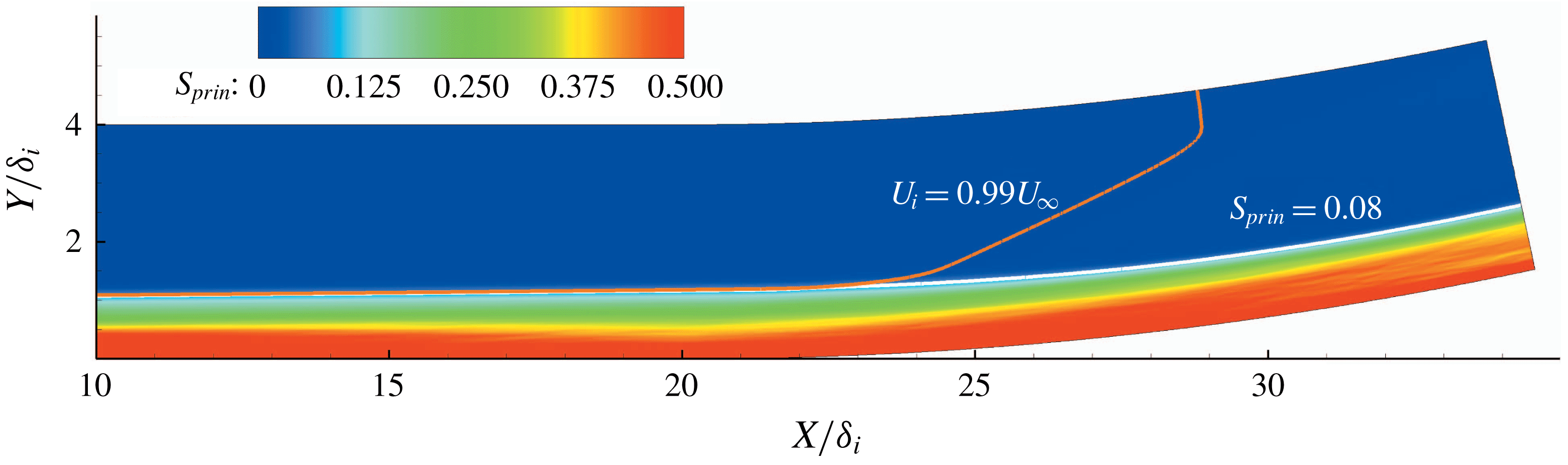
The contour map of the averaged static pressure of the supersonic concave boundary layer is given in figure 10. Obviously, the static pressure varies in both of the streamwise and wall-normal directions due to the downstream leaning compression waves. The wall-normal variation of static pressure leads to the wall-normal variation of the free-stream velocity, making it impossible to define the boundary-layer thickness using the conventional 99 % criterion, as shown in figure 11 where the outer edge defined by $99\,\%U_{\infty }$ is highlighted with an orange line. By assuming a constant static pressure within the boundary layer, Fernholzh & Finley (Reference Fernholzh and Finley1980) introduced a fictitious boundary-layer edge state, through which the boundary-layer thickness could be deduced. However, as we can find in figure 10, the static pressure varies within the boundary layer. Thus, the method introduced by Fernholzh & Finley (Reference Fernholzh and Finley1980) cannot be used here to define the boundary-layer thickness. It is necessary to have a new and more physically based method to define the boundary-layer thickness.

Figure 10.

Contour map of the averaged static pressure. The pressure is normalized with the free-stream parameter $\unicode[STIX]{x1D70C}_{\infty }U_{\infty }^{2}$ .

The method to define the boundary-layer thickness described in the present investigation is deduced from the distribution of principal strain rate. The contour map of the normalized mean principal strain rate $S_{prin}=\unicode[STIX]{x2202}(U_{t}/U_{\infty })/\unicode[STIX]{x2202}(y/\unicode[STIX]{x1D6FF}_{i})$ is given in figure 11. Clearly, the strain rate within the boundary layer is much larger than that in the main flow. Within the main flow, $S_{prin}$ is of the order of $10^{-4}$ , while within the boundary layer, $S_{prin}$ is much larger. Thus, it is possible to define the boundary-layer thickness physically by choosing an appropriate threshold for the principal strain rate.

Figure 11.

Contour map of the normalized principal strain rate $S_{prin}=\unicode[STIX]{x2202}(U_{t}/U_{\infty })/\unicode[STIX]{x2202}(y/\unicode[STIX]{x1D6FF}_{i})$ .

In figure 12(a), the streamwise variations of boundary-layer thickness under five appropriate $S_{prin}$ thresholds, which are $S_{prin}=0.06,0.07,0.08,0.09$ and 0.10, are given. Obviously, with different thresholds, the absolute values of the boundary-layer thickness vary, but the streamwise varying trends are similar. The variation of the boundary-layer thickness around the streamwise position of $x=2\unicode[STIX]{x1D6FF}_{i}$ is due to relaxation of the turbulent inflow generated by the digital-filter-based method. Here, we choose the threshold of $S_{prin}=0.08$ to define the boundary-layer thickness. The outer edges of the boundary layer defined by $S_{prin}=0.08$ and $S_{prin}=0.08$ are plotted in figure 11. As can be found in the figure, the edges defined by $99\,\%U_{\infty }$ and $S_{prin}=0.08$ are close in the flat-plate region and in the near field downstream of the turning point. Further downstream of $X\approx 23\unicode[STIX]{x1D6FF}_{i}$ , while $S_{prin}=0.08$ still defines a physical edge, the edge defined by $99\,\%U_{\infty }$ moves fast into the main stream. The streamwise variation of the streamwise velocity component at the outer edge is given in figure 12(b). In the flat-plate region, the edge velocity keeps a nearly constant value of $0.99U_{\infty }$ in the streamwise direction and this agrees well with the conventional 99 % criterion. In the concave region, the edge velocity decreases due to the compression.

Figure 12.

(a) Streamwise variations of boundary-layer thickness with different thresholds of normalized principal strain rate; (b) streamwise variation of streamwise velocity component at the outer edge of the boundary layer, which is defined by the threshold of $S_{prin}=0.08$ . The velocity is the normalized value by $U_{\infty }$ .

3.1.2 Wall friction

Streamwise variations of the skin friction coefficient $C_{f}=\unicode[STIX]{x1D70F}_{w}/(0.5\unicode[STIX]{x1D70C}_{\infty }U_{\infty }^{2})$ and the normalized friction velocity $U_{\unicode[STIX]{x1D70F}}=u_{\unicode[STIX]{x1D70F}}/U_{\infty }$ are given in figures 13(a) and 13(b), respectively. The streamwise increase of wall friction before $x=7\unicode[STIX]{x1D6FF}_{i}$ is due to the flow relaxation of the digital-filter-generated inflow. In the flat-plate region, a slow decrease of the wall friction is found. In the concave region, it rises with the wall turning, which is consistent with the finding given by Donovan et al. (Reference Donovan, Spina and Smits1994). However, if we carefully examine the curve, we find that the wall friction actually undergoes a slight drop in the vicinity of the turning point before it rises. This is mainly caused by the additional drag imposed by the suddenly emerged concave wall at the turning point, which leads to the decrease of near-wall velocity and the related wall friction. We will find in the subsequent discussion that the streamwise increase of skin friction in the concave region is mainly due to the promoted turbulence, which transports the high-momentum flow in the outer layer to the near-wall region and thus increases the near-wall velocity gradient in the wall-normal direction. However, at the turning point, the turbulence has not been effectively promoted to increase the near-wall velocity, which cannot compensate the velocity loss brought about by the additional drag. As a result, the streamwise velocity at $x=20\unicode[STIX]{x1D6FF}_{i}$ is finally reduced, as well as the skin friction. In the concave region, despite the streamwise increase of wall shear, the friction velocity decreases with the wall turning. Considering that the friction velocity is calculated with the relation $u_{\unicode[STIX]{x1D70F}}=\sqrt{\unicode[STIX]{x1D70F}_{w}/\unicode[STIX]{x1D70C}_{w}}$ , the decrease of the $U_{\unicode[STIX]{x1D70F}}$ is due to the increase of flow density.

Figure 13.

Streamwise variations of (a) friction coefficient $C_{f}=\unicode[STIX]{x1D70F}_{w}/(0.5\unicode[STIX]{x1D70C}_{\infty }U_{\infty }^{2})$ and (b) friction velocity normalized by $U_{\infty }$ .

3.1.3 Velocity profiles

Velocity profiles with inner and out scaling are shown in figures 14 and 15, respectively. Results are presented at five streamwise positions, $x=18.3\unicode[STIX]{x1D6FF}_{i}$ , $\unicode[STIX]{x1D6FC}=3.0^{\circ },6.0^{\circ },9.0^{\circ }$ and $11.0^{\circ }$ , where the streamwise position $x=18.3\unicode[STIX]{x1D6FF}_{i}$ is in the flat-plate region (the concave turning point is at $x=20\unicode[STIX]{x1D6FF}_{i}$ ) and $\unicode[STIX]{x1D6FC}=3.0^{\circ },6.0^{\circ },9.0^{\circ }$ and $11.0^{\circ }$ denote the local wall-turning angle in the concave region. Local friction velocities are used for the inner scaling, while local boundary-layer thicknesses are used for the outer scaling.

In figure 14, we find that at all streamwise positions the viscous sub-layer is well resolved and the profiles collapse for $y^{+}\lessapprox 8$ . Compared with the incompressible results of Barlow & Johnston (Reference Barlow and Johnston1988b ), where the profiles collapse well up to $y^{+}\approx 50$ , the impact of the concave curvature is found to be able to get down to the region much closer to the wall under the supersonic condition. From the buffer layer and above, the influence of the concave wall on the velocity profile is visible. Although it is still possible to find the logarithmic region with constant slope on the concave boundary layer, the slope decreases as the flow develops on the concave surface.

In figure 15(a), a general view of the velocity profiles throughout the boundary layer is presented. A zoom-in plot of profiles in the near-wall region is given in figure 15(b). Due to the compression, the streamwise velocity decreases for $y/\unicode[STIX]{x1D6FF}_{local}\gtrapprox 0.03$ as flow develops on the concave surface. However, in the near-wall region ( $y/\unicode[STIX]{x1D6FF}_{local}\lesssim 0.03$ ), the streamwise velocity increases with the wall turning, as shown in figure 15(b). This explains the streamwise increase of wall friction in the concave boundary layer. To facilitate subsequent analysis, we denote the region $y/\unicode[STIX]{x1D6FF}_{local}\lesssim 0.03$ as Layer A, and the region $y/\unicode[STIX]{x1D6FF}_{local}\gtrapprox 0.03$ as Layer B. Discussion of the physical cause of the alteration of the velocity profile in the concave region is given in § 4.

Figure 14.

Profiles with inner scaling at different streamwise positions. Streamwise positions in the concave region are denoted by the local turning angle of wall.

Figure 15.

Profiles with outer scaling at different streamwise positions. The wall-normal positions are normalized by the local boundary-layer thickness. (a) Velocity profiles within the height of $y/\unicode[STIX]{x1D6FF}_{local}<1.0$ ; (b) velocity profiles in the near-wall region within the height of $y/\unicode[STIX]{x1D6FF}_{local}<0.05$ .

3.1.4 Strain rate

To have a clear understanding of the mean shear stress throughout the concave boundary layer, profiles of the normalized principal strain rate $S_{prin}$ at five streamwise locations are presented in figure 16. In figure 16(a), the wall-normal position is scaled with inner variables, while in figure 16(b,c), the wall-normal position is scaled with the local boundary-layer thickness.

The principal strain rate $S_{prin}$ increases with the wall turning in the near-wall region (see figure 16 a,b). The shear stress within the viscous sub-layer is much higher than that in the logarithmic and wake regions. Outside the viscous sub-layer, $S_{prin}$ drops quickly. Different from the sub-layer, where the velocity gradient is maintained by the viscosity, the rapid growth of turbulence intensity outside the viscous sub-layer gradually makes the turbulent viscosity become the dominant factor in turbulent transportation and dissipation. The observed drop of $S_{prin}$ with the increase of wall-normal position in the buffer layer is the result of the raised Reynolds shear stress which quickly smooths the velocity gradient.

Considering that $S_{prin}$ has a much higher value in the near-wall region, profiles of $S_{prin}$ are given within different ranges of height to have a clear presentation of the principal strain data. In figure 16(b), the data are given in the near-wall region of $y/\unicode[STIX]{x1D6FF}_{local}<0.1$ , while in figure 16(c), the data are given within $0.1\leqslant y/\unicode[STIX]{x1D6FF}_{local}\leqslant 1.5$ . Combining figure 16(b,c), it is clear that, at different wall-normal positions, the streamwise varying trends of $S_{prin}$ are different as well. Three layers with different streamwise varying trends of $S_{prin}$ can be identified. This is consistent with the experimental finding given by Wang et al. (Reference Wang, Wang and Zhao2016a ). However, due to limit of spatial resolution of PIV, the high-shear region within the boundary layer is not revealed in their experiments and the layers cannot be clearly defined in their work. This can be clarified from the current numerical results, and the three layers are divided as follows.

1. (i) Layer I, located in the region of $y/\unicode[STIX]{x1D6FF}_{local}\lesssim 0.012$ and $S_{prin}$ grows with the wall turning.

2. (ii) Layer II, located in the region of $0.015\lesssim y/\unicode[STIX]{x1D6FF}_{local}\lesssim 0.2$ and $S_{prin}$ decreases with the wall turning.

3. (iii) Layer III, located in the region of $0.4\lesssim y/\unicode[STIX]{x1D6FF}_{local}\lesssim 0.8$ and $S_{prin}$ increase with the wall turning.

By combining figures 15 and 16, a complete scenario of the streamwise varying trend of velocity as well as its variation with height can be constructed. The streamwise increase of $S_{prin}$ in Layer I is closely related to the near-wall streamwise growth of velocity in Layer A. However, the thickness of Layer I is smaller than that of Layer A. This indicates that the streamwise growth rate of velocity varies with the wall-normal position in Layer A. In Layer I, the higher the wall-normal position is, the faster the velocity grows in the streamwise direction, offering a streamwise increasing trend of $S_{prin}$ . While in the region higher than Layer I, the velocity growth gradually slows down with the increase of wall-normal height and its streamwise varying trend is entirely reversed when it gets into the region higher than $y/\unicode[STIX]{x1D6FF}_{local}\approx 0.03$ (the lower edge of Layer B). As a consequence, a streamwise decreasing trend of $S_{prin}$ in Layer II is observed. Further, at positions higher than  $y/\unicode[STIX]{x1D6FF}_{local}\approx 0.2\sim 0.4$ , although the streamwise decreasing trend of velocity is maintained, it slows down gradually. Thus a higher wall-normal position can give a lower reduction rate of velocity, leading to the noted streamwise increasing trend of $S_{prin}$ in Layer III.

Figure 16.

Profiles of the normalized principal strain rate at different streamwise positions. The wall-normal coordinates are normalized in different ways. (a) The wall-normal positions are denoted by $y^{+}$ ; (b) data are given in the near-wall region within the height of $y/\unicode[STIX]{x1D6FF}_{local}<0.1$ ; (c) data are given within the height of $0.1\leqslant y/\unicode[STIX]{x1D6FF}_{local}\leqslant 1.5$ .

An averaged contour map of the normalized bulk dilatation  $(\unicode[STIX]{x1D735}\boldsymbol{\cdot }\boldsymbol{U})\boldsymbol{\cdot }\unicode[STIX]{x1D6FF}_{i}/U_{\infty }$ is given in figure 17. The trace of the first compression wave induced by the concave wall is clearly extracted in the contour map. It seems that the bulk dilatation is very sensitive in extracting simple waves. The compression wave is curved within the boundary layer and in the main flow it extends in a straight manner towards the downstream. The negative value noted in the region downstream of the first compressive wave indicates that the flow is compressed and the flow farther away from the wall is subjected to more severe compression.

Figure 17.

Contour map of the normalized bulk dilatation $(\unicode[STIX]{x1D735}\boldsymbol{\cdot }\boldsymbol{U})\boldsymbol{\cdot }\unicode[STIX]{x1D6FF}_{i}/U_{\infty }$ .

3.3.1 Instantaneous flow structures

An instantaneous distribution of density in an $xy$ plane of the supersonic concave turbulent boundary layer is given in figure 22. A streamwise increase of density brought about by the compressive waves can be clearly seen. The streamwise variation of turbulent structures along the concave wall is similar to the flow-visualization results given by Wang & Wang (Reference Wang and Wang2016). In the concave region, the vortex structures appear to have smaller scales than those in the flat-plate region. Considering that the shock waves could complicate the flow, the absence of shock waves in the present study might facilitate the direct study of the physical impacts of the streamwise concave curvature and the related adverse pressure gradient on boundary layer.

Figure 22.

Instantaneous distribution of density in the supersonic concave turbulent boundary layer.

An overall view of the instantaneous Euler vortices extracted with the $\unicode[STIX]{x1D6E5}$ criterion (Chakraborty, Balachandar & Adrian Reference Chakraborty, Balachandar and Adrian2005; Chong, Perry & Cantwell Reference Chong, Perry and Cantwell1990), which clearly shows the three-dimensional evolution of the vortex structures under concave curvature, is given in figure 23(a). For $d/\unicode[STIX]{x1D6FF}_{i}\leqslant 0.4$ , zoom-in views of the extracted vortices in the flat-plate and curved regions are given in figures 23(b) and 23(c), respectively. The differences between the vortices in the flat-plate and curved regions are notable. Since the results are presented in the region relatively close to the wall, quasi-streamwise vortices, whose existence is a typical feature of near-wall turbulence, can be frequently noticed in the flat-plate region (see figure 23 b). However, in the concave region (see figure 23 c), turbulence is dominated by the well-developed hairpin vortices, which means that coherent large-scale motions are getting closer to the wall due to the concave curvature. The curvature gives higher vortex production, and as a consequence, much denser distributed vortices in the curved region are noticed.

Figure 23.

Instantaneous vortex structures extracted by the $\unicode[STIX]{x1D6E5}$ criterion with $\unicode[STIX]{x1D6E5}=0.0015$ lower than the wall-normal height of $d/\unicode[STIX]{x1D6FF}_{i}=0.4$ . The iso-surfaces are coloured by the streamwise velocity. (a) An overall view of the vortex structures from the flat-plate region to the concave, (b) a zoomed-in view in the flat-plate region, (c) a zoomed-in view in the concave region.

In figure 24, cross-flow slices are shown for the instantaneous distribution of streamwise velocity at six streamwise positions. Two slices are given in the flat-plate region and four in the curved region. It is clear that the general distribution of the streamwise velocity in the concave region, especially at streamwise positions of $\unicode[STIX]{x1D6FC}=9.0^{\circ }$ and $\unicode[STIX]{x1D6FC}=11.0^{\circ }$ , differs significantly from that in the flat-plate region. The low-momentum fluid which initially accumulated in the near-wall region is found to have a more evident tendency to move outwards under the impact of the concave curvature. The momentum transportation seems to be enhanced in the concave region. To have a more detailed discussion on the instantaneous flow field, two cross-sectional slices presented in figure 24 are further extracted, as shown in figure 25. One slice is in the flat-plate region at $x/\unicode[STIX]{x1D6FF}_{i}=18.3$ and the other is in the concave region at $\unicode[STIX]{x1D6FC}=11.0^{\circ }$ . Contour maps of the instantaneous streamwise velocity as well as stream traces are presented in the figure. Bulges due to the outwards-moving trend of the low-momentum flow can be seen in both of the flat-plate and the concave regions, and it bulges further into the main stream in the concave region than that in the flat-plate region. Along with the bulge of the low-momentum flow, large-scale streamwise swirls can be clearly seen through the pattern of the stream traces at $\unicode[STIX]{x1D6FC}=11.0^{\circ }$ (see figure 25 b). While in the flat-plate region, the streamwise swirls seem to be more randomly distributed and on a smaller scale (see figure 25 a). The obvious differences in the velocity distribution and stream trace pattern between the slices extracted at $x/\unicode[STIX]{x1D6FF}_{i}=18.3$ and at $\unicode[STIX]{x1D6FC}=11.0^{\circ }$ suggest the existence of large-scale longitudinal roll cells, which were first found by Barlow & Johnston (Reference Barlow and Johnston1988a ,Reference Barlow and Johnston b ) in the incompressible concave boundary layer. According to Barlow & Johnston (Reference Barlow and Johnston1988a ,Reference Barlow and Johnston b ), it is hard to define the roll cells in the turbulent boundary layer due to the complexity of the flow. The roll cells do not have a concentrated vorticity and they usually vary with time and streamwise position. More supportive evidence of the large-scale roll cells can be found by extracting instantaneous streamwise vortices and probability density distributions of the streamwise vorticity, as given below.

Figure 24.

Instantaneous contour maps of streamwise velocity at different streamwise positions.

Figure 25.

Contours of the instantaneous streamwise velocity and stream traces in two cross-sectional planes: (a) $x/\unicode[STIX]{x1D6FF}_{i}=18.3$ , (b) $\unicode[STIX]{x1D6FC}=11.0^{\circ }$ .

For vortex extraction, a modified swirling-strength parameter $\unicode[STIX]{x1D706}_{s,x}$ introduced by Wu & Christensen (Reference Wu and Christensen2006) is used. $\unicode[STIX]{x1D706}_{s,x}$ is defined as

where, $\unicode[STIX]{x1D714}_{x}=0.5(\unicode[STIX]{x2202}w/\unicode[STIX]{x2202}y-\unicode[STIX]{x2202}v/\unicode[STIX]{x2202}z)\cdot \unicode[STIX]{x1D6FF}_{i}/U_{\infty }$ is the dimensionless streamwise vorticity and $\unicode[STIX]{x1D706}_{ci}$ is the imaginary part of the complex eigenvalue of the local velocity-gradient tensor (Zhou et al. Reference Zhou, Adrian, Balachandar and Kendall1999; Elsinga et al. Reference Elsinga, Adrian, Oudheusden and Van Scarano2010). The sign of the vorticity is used to distinguish the direction of rotation. In the cross-sectional plane and for the streamwise vortices, the streamwise swirling strength $\unicode[STIX]{x1D706}_{ci}(y,z)$ considers only the spanwise and wall-normal velocity components and is defined as the imaginary part of the eigenvalues of $J_{vw}$

Contour maps of the instantaneous swirling-strength parameter $\unicode[STIX]{x1D706}_{s,x}$ corresponding to the velocity distributions presented in figure 25 are given in figure 26. As can be found in the figure, throughout the boundary layer the number and strength of the streamwise vortices in the concave region are higher than in the flat-plate region. The streamwise swirling is intensified by the concave curvature. The more densely distributed streamwise vortices observed here are consistent with the results given in figure 23 where a much larger number of hairpins is observed in the concave region. Combining the stream traces presented in figure 25 and streamwise vortices in figure 26, it is reasonable to deduce that it is actually the accumulations of a large number of small-scale streamwise vortices with a similar sense of rotation and their combined effects that lead to the formation of the large-scale roll cells.

In figure 27, distributions of probability density of the dimensionless streamwise vorticity $\unicode[STIX]{x1D714}_{x}$ at two wall-normal positions ( $y/\unicode[STIX]{x1D6FF}_{i}=0.008$ and $y/\unicode[STIX]{x1D6FF}_{i}=0.23$ ) are presented. The results show promotion of the streamwise swirling in the concave boundary layer. At both wall-normal positions the boundary layer in the concave region tends to have a larger streamwise vorticity. More dominant promotion of streamwise vorticity is found in the near-wall position. This statistical result supports the deduction from figure 25. It is because of the combined effects of these streamwise vortices which are intensified in the concave boundary layer that forms the large-scale roll cells. Through intensifying the pre-existing streamwise vortices and producing more, the overall streamwise swirling is promoted. Typical features of the roll cells are the clear spanwise variations of turbulent structure. The bulges of the low-speed flow are direct results of the promoted streamwise swirling which gives the low-speed flow a stronger tendency to move outwards and induces the high-speed flow to move towards the wall.

Figure 26.

Contours of instantaneous swirling-strength parameter $\unicode[STIX]{x1D706}_{s,x}$ at two streamwise positions: (a) $x/\unicode[STIX]{x1D6FF}_{i}=18.3$ , (b) $\unicode[STIX]{x1D6FC}=11.0^{\circ }$ . Contour lines of $u/U_{\infty }=0.5$ and 0.8 are also plotted.

Figure 27.

Probability density distributions of dimensionless streamwise vorticity $\unicode[STIX]{x1D714}_{x}$ at two wall-normal positions: (a) $y/\unicode[STIX]{x1D6FF}_{i}=0.008$ in the viscous sub-layer, (b) $y/\unicode[STIX]{x1D6FF}_{i}=0.23$ around the outer edge of the log region. Symbols are used to discriminate the curves acquired at different streamwise positions.

By checking the directions of swirling in the plane of $\unicode[STIX]{x1D6FC}=11.0^{\circ }$ , it can be observed that stream traces on each side of one low-momentum bulge actually swirl in counter directions, as shown in the circled region of figure 25(b). This resembles a flow field with Görtler vortices. It has been generally recognized that the Görtler instability introduced by the streamline concave curvature has a significant impact on both turbulent and laminar boundary layers. In the laminar boundary layer the Görtler instability presents itself as counter-rotating streamwise vortices, while in the turbulent boundary layer it has similar impacts on the flow by promoting the streamwise swirling. Although it is impossible to find the Görtler vortices in a turbulent boundary layer, the intensification of streamwise vortices found here indicates the contribution of the Görtler instability to the formation of large-scale roll cells in the supersonic flow. This is similar to that found that by Barlow & Johnston (Reference Barlow and Johnston1988a ,Reference Barlow and Johnston b ) in the incompressible concave boundary layer.

To find out more details regarding how these large-scale roll cells are formed, an instantaneous iso-surface of the streamwise velocity at $u/U_{\infty }=0.55$ is obtained, as shown in figure 28. The iso-surface is coloured by the wall-normal height. Dominant stronger outwards-moving trend of the low-momentum flow in the concave region than that in the flat-plate region can be observed in the figure, indicating the significant role of the large-scale roll cells in promoting momentum transportation. It can also be found in figure 28 that the bulges of iso-surface actually evolve from the streamwise extended structures (denoted by A, B and C) formed in the flat-plate boundary layer, which remind us of the very-large-scale motions(VLSMs) and their possible relationship with the large-scale roll cells found in the concave boundary layer.

Figure 28.

Iso-surface of streamwise velocity at $u/U_{\infty }=0.55$ coloured by wall-normal position.

Another view of these streamwise extended structures, which is acquired at $y/\unicode[STIX]{x1D6FF}_{i}=0.12$ in the logarithmic region (the corresponding $y^{+}$ is 38 in the flat region), is given in figure 29(a). Vortices extracted with $\unicode[STIX]{x1D6E5}=0.0015$ and contours of the streamwise velocity are presented in the figure. Similar to what is shown in figure 28, three elongated low-momentum regions which start in the flat-plate region and persist for the entire streamwise length of the viewing window can be clearly observed. Despite the meandering of the low-speed structures in the concave region, the extracted vortices are seen to distribute mainly along these low-speed structures, suggesting the dominant contribution of the low-speed structures in the generation of vortices. A zoomed-in view of the flow field within $15\leqslant x/\unicode[STIX]{x1D6FF}_{i}\leqslant 25$ is given in figure 29(b), where contour lines of the streamwise velocity at $u_{t}/U_{\infty }=0.6$ are extracted. The streamwise swirling-strength parameter $\unicode[STIX]{x1D706}_{s,y}$ in the $xz$ plane is also calculated by using a relation similar to (3.1), and patches with $|\unicode[STIX]{x1D706}_{s,y}|\geqslant 0.2$ are presented in the figure. It can be found in figure 29(b) that the extracted vortices are mostly distributed along the streamwise extended low-momentum structures. For any of the three low-speed structures, negative $\unicode[STIX]{x1D706}_{s,y}$ can be frequently observed around the upper edges while positive $\unicode[STIX]{x1D706}_{s,y}$ is usually found around the lower edges. The counter-rotation of these vortices on two sides of the elongated low-speed region indicates streamwise aligned one- and two-legged hairpin vortices and the related packets (Adrian, Meinhart & Tomkins Reference Adrian, Meinhart and Tomkins2000; Elsinga et al. Reference Elsinga, Adrian, Oudheusden and Van Scarano2010). This also indicates that the streamwise extended low-speed structures in the logarithmic layer are VLSMs.

Figure 29.

Contours of instantaneous field at wall-normal heights of $y/\unicode[STIX]{x1D6FF}_{i}=0.12$ (the corresponding $y^{+}$ is 38 at the streamwise position of $x=18.3\unicode[STIX]{x1D6FF}_{i}$ and 50 at $\unicode[STIX]{x1D6FC}=6.0^{\circ }$ ). (a) Contours of streamwise velocity and vortex structures extracted with $\unicode[STIX]{x1D6E5}=0.0015$ . (b) Contour lines of streamwise velocity with $u_{t}/U_{\infty }=0.6$ and patches of swirling-strength parameter $|\unicode[STIX]{x1D706}_{s,y}|\geqslant 0.2$ ; the blue and red contours represent the positive and negative values of $|\unicode[STIX]{x1D706}_{s,y}|$ , respectively.

As has been revealed in many previous reports regarding both supersonic and subsonic turbulent boundary layers (Kim & Adrian Reference Kim and Adrian1999; Hutchins & Marusic Reference Hutchins and Marusic2007; Ringuette, Wu & Martin Reference Ringuette, Wu and Martin2008; Lee & Sung Reference Lee and Sung2011), the VLSMs are brought about by the combination of adjacent hairpin packets. The momentum transportation within the turbulent boundary layer is closely related to the induced velocity from the swirling of the hairpins which are organized in packets. While the high-momentum flow in the outer layer tends to be induced to move towards the wall, the near-wall low-momentum flow is induced to move away from the wall. The streamwise elongated regions of momentum deficit are the direct results of the streamwise aligned hairpin packets (Adrian et al. Reference Adrian, Meinhart and Tomkins2000). The bulges of iso-surface of the streamwise velocity observed in figure 28 are brought about by the outward-moving low-momentum flow. In the concave region, the low-momentum flow bulge is much higher, suggesting that the large-scale motion and the momentum transportation are intensified through the formation of roll cells in the concave boundary layer. Despite the stronger outward-moving trend, these bulges remain streamwise extensions of the VLSMs formed in the flat-plate boundary layer.

Thus, it can be confirmed that the large-scale roll cells found in the concave boundary layer actually originate from the VLSMs formed in the flat-plate boundary layer. Hairpin vortices, which are usually organized in packets, populate the VLSMs. The legs of the hairpin vortices are usually streamwise extended vortices. We have shown that the streamwise vortices can be significantly intensified in the concave boundary layer. After the VLSMs formed in the flat boundary layer get into the concave region, the large number of streamwise extended vortices within the hairpin packets are strengthened by the Görtler instability, and more hairpin vortices are generated around the edges of the low-speed regions. On two sides of the low-speed region, the hairpin vortices tend to have a counter sense of rotation. After the intensification of these vortices and more are generated by the Görtler instability, their accumulations and combined effect lead to larger-scale streamwise swirls, as found in figure 25(b) and the roll cells observed by Barlow & Johnston (Reference Barlow and Johnston1988a ,Reference Barlow and Johnston b ). The roll cells can significantly enhance the momentum transportation between the inner and outer layers and make the velocity iso-surface in the concave boundary-layer bulges higher than that in the flat-plate boundary layer. Stronger momentum transportation makes for stronger shear between the low- and high-momentum region. This also contributes to the generation of hairpin vortices in the low-speed region in the concave boundary layer, as can be seen in figures 23 and 29(a).

The impacts of the roll cells on the near-wall turbulence can be seen in figure 30(a), where a contour map of instantaneous velocity at the wall-normal height of $y/\unicode[STIX]{x1D6FF}_{i}=0.02$ (the corresponding $y^{+}$ is 6.5 in the flat region) in the sub-layer is given. Due to the large-scale roll cells, the near-wall structures of the turbulent boundary layer are dramatically altered. The streamwise elongated low-speed streaks can be clearly seen in the flat-plate region. In the concave region, the streaks are severely interrupted and truncated by the frequently occurring high-speed patches, making the scales of these streaks smaller in both the streamwise and spanwise directions. The frequently noted high-speed patches in the curved region imply that, while the outward motion is enhanced in the concave boundary layer, the inward motion is significantly promoted as well, through which the high-momentum flow is brought to the near-wall region. Although the turbulent structures in figures 30(a) and 29(a) are evidently different, the faint superimposed footprints of the VLSM and the large-scale roll cells in the near-wall region could be observed if we carefully examine their flow structures.

At the higher wall-normal position, as shown in figure 30(b) where an instantaneous distribution of streamwise velocity at $y/\unicode[STIX]{x1D6FF}_{i}=0.33$ (the corresponding $y^{+}$ is 100 in the flat region) is given, the impact of the roll cells is also obvious. In the curved region, the low-momentum flow is found to have a higher tendency to move outwards. While the turbulence is dominated by the high-momentum flow in the flat-plate region, downstream of $x/\unicode[STIX]{x1D6FF}_{i}=25$ the turbulence at the same wall-normal height is dominated by the flow with much lower velocity.

Figure 30.

Contours of the streamwise velocity in wall-parallel planes at wall-normal heights of (a) $y/\unicode[STIX]{x1D6FF}_{i}=0.02$ (the corresponding $y^{+}$ is 6.5 at the streamwise positions of $x=18.3\unicode[STIX]{x1D6FF}_{i}$ in the flat-plate region and 7.5 at $\unicode[STIX]{x1D6FC}=6.0^{\circ }$ in the concave region), and (b) $y/\unicode[STIX]{x1D6FF}_{i}=0.33$ (the corresponding $y^{+}$ is 100 at the streamwise position of $x=18.3\unicode[STIX]{x1D6FF}_{i}$ and 130.24 at $\unicode[STIX]{x1D6FC}=6.0^{\circ }$ ).

The formation of large-scale roll cells is the main cause of the promotion of turbulence level. How the turbulence level is promoted in the concave turbulent boundary layer is discussed in § 3.3.2.

3.3.2 Quadrant decomposition

Due to the induced velocity from the swirl of the hairpin vortices which are organized in packets within the VLSMs and the large-scale roll cells, different turbulence events are induced. The quadrant decomposition technique (Lu & Willmarth Reference Lu and Willmarth1973; Pokrajac et al. Reference Pokrajac, Campbell, Nikora, Manes and Mcewan2007; Tichenor et al. Reference Tichenor, Humble and Bowersox2013), which has been widely used to study dynamic boundary-layer events, is useful for the present investigation. With quadrant decomposition, the fluctuation data can be divided into four quadrants in the $xy$ plane: outward interaction (Q1 event, $u^{\prime }>0$ , $v^{\prime }>0$ ); ejection (Q2 event, $u^{\prime }<0$ , $v^{\prime }>0$ ); inward interaction (Q3 event, $u^{\prime }<0$ , $v^{\prime }<0$ ); and sweep (Q4 event, $u^{\prime }>0$ , $v^{\prime }<0$ ), where $u^{\prime }$ and $v^{\prime }$ are the streamwise and wall-normal velocity fluctuations.

Quadrant decomposition results at two wall-normal positions, which are $y/\unicode[STIX]{x1D6FF}_{i}=0.008$ in the sub-layer and $y/\unicode[STIX]{x1D6FF}_{i}=0.04$ in the buffer layer, are presented in figure 31. At each wall-normal position, scatter plots of the decomposition at three streamwise positions, which are $x=18.3\unicode[STIX]{x1D6FF}_{i}$ , $\unicode[STIX]{x1D6FC}=3.0^{\circ }$ and $\unicode[STIX]{x1D6FC}=9.0^{\circ }$ , are given.

Clearly, at $y/\unicode[STIX]{x1D6FF}_{i}=0.008$ , the scattered area grows with the wall turning, as shown in figure 31(a–c). The probability of having positive or negative $v^{\prime }$ with an absolute value larger than $1.0\,\%U_{\infty }$ is significantly increased as the flow develops on the concave surface. For the streamwise fluctuation $u^{\prime }$ , the probability of having a positive value larger than $15.0\,\%U_{\infty }$ is increased with the wall turning. But the absolute value of negative $u^{\prime }$ is mostly confined to be smaller than $10.0\,\%U_{\infty }$ . The negative streamwise fluctuations are not significantly enhanced.

At the higher wall-normal position of $y/\unicode[STIX]{x1D6FF}_{i}=0.04$ , as shown in figure 31(d–f), the scattered areas are much larger than those at $y/\unicode[STIX]{x1D6FF}_{i}=0.008$ . It should be noted that the vertical axis ranges for $v^{\prime }/U_{\infty }$ in figure 31(d–f) are different from those in (a–c). The scattered area is also found to be increased with the wall turning, which is similar to the case at $y/\unicode[STIX]{x1D6FF}_{i}=0.008$ . The probability of having high positive or negative values of $u^{\prime }$ is not significantly increased. The streamwise increase of the scattered area is mostly attributed to the variation in the distribution of $v^{\prime }$ whose probability of having absolute values larger than $5.0\,\%U_{\infty }$ is evidently increased in the concave region.

Through the analysis of figure 31, it is noticed that the wall-normal fluctuation at both heights is significantly promoted in the concave boundary layer. Combining this with the findings in § 3.3.1, it is concluded that, while the large-scale roll cells make a significant contribution to the promotion of the wall-normal motion (both inward and outward motions), their impact on the streamwise motion is relatively weak. The ejection and sweep events are strengthened due to the promotion of wall-normal motion, which causes more intense momentum transfer between the inner and outer layers in the concave boundary layer.

Figure 31.

Scatter plots of the Reynolds stress quadrant decomposition. (a–c) At the wall-normal position of $y/\unicode[STIX]{x1D6FF}_{i}=0.008$ in the viscous sub-layer; (d–f) at the wall-normal position of $y/\unicode[STIX]{x1D6FF}_{i}=0.04$ in the buffer layer. (a,d) At the streamwise position of $x=18.3\unicode[STIX]{x1D6FF}_{i}$ ; (b,e) at the streamwise position of $\unicode[STIX]{x1D6FC}=3.0^{\circ }$ ; (c,f) at the streamwise position of $\unicode[STIX]{x1D6FC}=9.0^{\circ }$ .

The scatter plots also suggest that the Q2 and Q4 events play more important parts in the Reynolds stress. Following Tichenor et al. (Reference Tichenor, Humble and Bowersox2013), to further evaluate the respective contributions of different events, the average of $u^{\prime }v^{\prime }$ for each quadrant can be calculated.

where, $N$ is the number of total samples, $N_{i}$ is the sample number for the $i$ th quadrant. The sum of averages of $u^{\prime }v^{\prime }$ for four quadrants is the Reynolds shear stress.

The profiles of averaged $u^{\prime }v^{\prime }$ normalized by $U_{\infty }^{2}$ for the four quadrants at $x=18.3\unicode[STIX]{x1D6FF}_{i}$ in the flat region are given in figure 32(a). For all four quadrants of the flat-plate boundary layer, $(uv)_{i}/U_{\infty }^{2}$ peaks occur around the wall-normal position of $y/\unicode[STIX]{x1D6FF}_{i}=0.1$ (corresponding to $y^{+}=32$ ). Negative values of the Q2 and Q4 events are much larger than those of the Q1 and Q3 events. The respective contribution of each quadrant can be further evaluated by normalizing the averaged $u^{\prime }v^{\prime }$ with total Reynolds shear stress $(uv)_{ave}$ . The profiles are given in figure 32(b). Obviously, Q2 and Q4 events contribute predominantly to the mean Reynolds shear stress throughout the boundary layer. In the near-wall region, the Q4 event contributes the majority of Reynolds stress, indicating that the near-wall turbulence is mainly generated by the sweep event. Its contribution decreases fast with the wall-normal height in the region from the wall to $y/\unicode[STIX]{x1D6FF}_{i}=0.1$ , while simultaneously, the contribution of Q2 increases quickly, taking the most important role in the Reynolds shear stress. Further away from the wall, with the importance of the Q4 event in the Reynolds shear stress being gradually weakened with the wall-normal height, the importance of Q2 event is gradually promoted.

Figure 32.

Quadrant decomposition analysis of the Reynolds stress at the streamwise position of $x=18.3\unicode[STIX]{x1D6FF}_{i}$ in the flat-plate region. (a) Profiles of quadrant decomposed Reynolds stress; (b) contributions of different events to the mean Reynolds stress.

Considering the importance of Q2 and Q4 events, profiles of the quadrant decomposed Q2 and Q4 Reynolds stress at five streamwise positions are given in figure 33. Obviously, both Q2 ejection and Q4 sweep events are significantly strengthened in the concave boundary layer. Both the ejection and sweep events are correlated with the wall-normal motions. The strengthened ejection and sweep events are the direct results of the large-scale roll cells which induce the high-momentum flow to move inward while induce the low-momentum flow to move outward at the same time. The strengthening of ejection and sweep events noted here is also responsible for the streamwise increase of Reynolds shear stress that has been pointed in § 3.2. While the Reynolds shear stress is closely related to the turbulence production, the turbulence intensity is promoted. In addition, it also can be found in figure 33 that, along with the streamwise increase of sweep and ejection events, their peaking positions are gradually moving outwards as well. This suggests a higher turbulence production in the outer layer in the supersonic concave turbulent boundary layer. As a result, second bumps are introduced into the profiles for the streamwise and spanwise turbulence intensities. For the same reason, peak positions in the profiles of the wall-normal turbulence intensity and the Reynolds shear stress move outwards with the wall turning as well.

Figure 33.

Profiles of quadrant decomposed Reynolds stress at different streamwise positions. (a) Q2 event; (b) Q4 event.

To further identify the boundary-layer events in the $xz$ plane, scatter plots of the quadrant decomposition for $u^{\prime }$ and $w^{\prime }$ at two wall-normal positions, which are $y/\unicode[STIX]{x1D6FF}_{i}=0.008$ in the viscous sub-layer and $y/\unicode[STIX]{x1D6FF}_{i}=0.228$ in the logarithmic layer, are given in figure 34, where $w^{\prime }$ is the spanwise velocity fluctuation. At each wall-normal position, scatter plots at three streamwise positions, which are $x=18.3\unicode[STIX]{x1D6FF}_{i}$ , $\unicode[STIX]{x1D6FC}=3.0^{\circ }$ and $\unicode[STIX]{x1D6FC}=9.0^{\circ }$ , are given. It can be found in the figure that at both wall-normal positions the spanwise fluctuation $w^{\prime }$ tends to have a larger value with the wall turning. The promotion of the spanwise fluctuation in the concave boundary layer is consistent with our findings in § 3.3.1 where large-scale longitudinal roll cells are identified. This also explains the streamwise increase of spanwise turbulence intensity.

Figure 34.

Scatter plots of the quadrant decomposition in the $xz$ plane. (a–c) At the wall-normal position of $y/\unicode[STIX]{x1D6FF}_{i}=0.008$ in the viscous sub-layer; (d–f) at the wall-normal position of $y/\unicode[STIX]{x1D6FF}_{i}=0.228$ in the logarithmic layer. (a,d) At the streamwise position of $x=18.3\unicode[STIX]{x1D6FF}_{i}$ ; (b,e) at the streamwise position of $\unicode[STIX]{x1D6FC}=3.0^{\circ }$ ; (c,f) at the streamwise position of $\unicode[STIX]{x1D6FC}=9.0^{\circ }$ .

3.3.3 Two-point spatial correlation

To check the response of large-scale coherent motions to the streamwise concave curvature, two-point spatial correlation maps for the streamwise velocity component are calculated in the wall-parallel and $xy$ planes. In the wall-parallel plane, the spatial correlation is calculated with the relation:

where, the subscript ‘0’ denotes the reference position, $\unicode[STIX]{x0394}x$ and $\unicode[STIX]{x0394}z$ are the in-plane streamwise and spanwise separations, respectively. The correlation results in the wall-parallel planes with $y^{+}=10$ and $y^{+}=100$ ( $y^{+}$ is calculated using the friction velocity $u_{\unicode[STIX]{x1D70F}}$ at the reference streamwise position) are given in figures 35 and 36, respectively. In each plane, the results at four reference streamwise positions are presented, which are $x=18.3\unicode[STIX]{x1D6FF}_{i}$ , $\unicode[STIX]{x1D6FC}=3.0^{\circ }$ , $\unicode[STIX]{x1D6FC}=6.0^{\circ }$ and $\unicode[STIX]{x1D6FC}=9.0^{\circ }$ .

Obviously, the iso-contours are streamwise extended, which is a typical feature of the correlation map in the wall-parallel plane. It reflects the existence of low-speed streaks, but its streamwise dimension does not strictly reveal the streamwise length of the streak due to its meandering nature (Hutchins & Marusic Reference Hutchins and Marusic2007). Clearly, the streamwise correlation varies with the wall turning at both wall-normal positions. In the plane of $y^{+}=10$ (see figure 35), the streamwise correlation increases from $x=18.3\unicode[STIX]{x1D6FF}_{i}$ in the flat-plate region to $\unicode[STIX]{x1D6FC}=6.0^{\circ }$ in the concave region. Further downstream at $\unicode[STIX]{x1D6FC}=9.0^{\circ }$ , it is evidently decreased. This is mainly attributed to the large number of high-momentum patches induced by the large-scale roll cells from the outer layer (see figure 30(a) in the region from $x/\unicode[STIX]{x1D6FF}_{i}=27$ to 31), which truncate the near-wall streaks and diminish the streamwise correlation in the concave region. At the higher wall-parallel plane with $y^{+}=100$ , the streamwise dimension of the iso-contour at $x=18.3\unicode[STIX]{x1D6FF}_{i}$ is obviously smaller than at $y^{+}=10$ . However, the length of the iso-contour increases persistently in the streamwise direction. At the streamwise position of $\unicode[STIX]{x1D6FC}=9.0^{\circ }$ , the streamwise correlation of the turbulence in the plane $y^{+}=100$ is much higher than that in the plane $y^{+}=10$ . The higher streamwise correlation at $y^{+}=100$ is mainly attributed to the large-scale roll cells which make the turbulence more streamwise correlated in the low wake region.

Figure 35.

Two-point spatial correlation maps in the wall-parallel plane at $y^{+}=10$ . Twelve levels between $-0.1$ and 1.0 with an increment of 0.1 are shown. The black solid contour line plotted is for the correlation value of 0.1. Results are acquired at four reference streamwise positions: (a) $x=18.3\unicode[STIX]{x1D6FF}_{i}$ , (b) $\unicode[STIX]{x1D6FC}=3.0^{\circ }$ , (c) $\unicode[STIX]{x1D6FC}=6.0^{\circ }$ , (d) $\unicode[STIX]{x1D6FC}=9.0^{\circ }$ .

Figure 36.

Two-point spatial correlation maps in the wall-parallel plane of $y^{+}=100$ . Twelve levels between $-0.1$ and 1.0 with increments of 0.1 are shown. The black solid contour line plotted is for the correlation value of 0.1. Results are acquired at different streamwise reference positions: (a) $x=18.3\unicode[STIX]{x1D6FF}_{i}$ , (b) $\unicode[STIX]{x1D6FC}=3.0^{\circ }$ , (c) $\unicode[STIX]{x1D6FC}=6.0^{\circ }$ , (d) $\unicode[STIX]{x1D6FC}=9.0^{\circ }$ .

In addition to the variation of streamwise dimension of the iso-contour, the spanwise dimension is also found to vary both in the streamwise and wall-normal directions, as shown in figures 35 and 36. To have a clearer evaluation of the iso-contour width, the spanwise profiles of the two-point correlation at five streamwise reference positions are extracted. Similar to those given in figures 35 and 36, the correlation results are acquired at two wall-normal positions, which are $y^{+}=10$ and $y^{+}=100$ , as shown in figure 37. Two methods of normalization for the spanwise dimension are employed. In figure 37(a,c), the width is denoted by $z^{+}$ , and in figure 37(b,d), the width is normalized with the inflow boundary-layer thickness $\unicode[STIX]{x1D6FF}_{i}$ to present the absolute value.

With inner scaling, the iso-contour width denoted by $z^{+}$ is evidently increased with the wall turning in both wall-parallel planes, as given in figure 37(a,c). The absolute value of width is also found to increase in the streamwise direction in the wall-parallel plane with $y^{+}=10$ . But in the higher plane, its streamwise variation is relatively weak. Thus the noted streamwise growth of the iso-contour width in figure 37(c) is mainly attributed to the streamwise decrease of the friction velocity.

Figure 37.

Spanwise profiles of two-point spatial correlation $R_{uu}$ at different streamwise positions. The results are presented for various wall-normal positions: (a,b) $y^{+}=10$ ; (c,d) $y^{+}=100$ . Different normalization methods are used for the spanwise width: (a,c) the spanwise width is denoted by $z^{+}$ ; (b,d) the spanwise width is denoted by $z/\unicode[STIX]{x1D6FF}_{i}$ .

Two-point spatial correlation maps in the $xy$ plane are also calculated by using the relation

The correlations at two wall-normal reference positions, which are $y^{+}=5$ and $y^{+}=50$ , are calculated, as given in figures 38 and 39. At each wall-normal position, results at four streamwise positions are presented.

It is clear that all of the iso-contours are seen to possess a forward-leaning elliptical distribution, which is consistent with previous studies regarding turbulent boundary layers (Humble et al. Reference Humble, Peltier and Bowersox2012; Tichenor et al. Reference Tichenor, Humble and Bowersox2013; Wang et al. Reference Wang, Wang and Zhao2016a ). At the higher wall-normal position, the iso-contours are found to lean farther away from the wall. Since the leaning angle of an iso-correlation map represents the growth angle of a hairpin packet, which is defined by the envelope of the within hairpin heads (Adrian et al. Reference Adrian, Meinhart and Tomkins2000; Wang, Wang & Zhao Reference Wang, Wang and Zhao2017), the variation of the leaning angle indicates that the growth angle of the hairpin packet at $y^{+}=50$ is larger than at $y^{+}=10$ . In addition, the non-dimensional spatial extent of the iso-contour appears to be larger at the higher wall-normal position, suggesting that larger, more highly correlated turbulent structures are present in the outer region of the boundary layer.

Figure 38.

Two-point spatial correlation maps in the $xy$ plane at the wall-normal reference position of $y^{+}=5$ . The streamwise reference position varies: (a) $x=18.3\unicode[STIX]{x1D6FF}_{i}$ , (b) $\unicode[STIX]{x1D6FC}=3.0^{\circ }$ , (c) $\unicode[STIX]{x1D6FC}=6.0^{\circ }$ , (d) $\unicode[STIX]{x1D6FC}=9.0^{\circ }$ . The outer (minimum) correlation value is 0.2.

Figure 39.

Two-point spatial correlation maps in the $xy$ plane at the wall-normal reference position of $y^{+}=50$ . The streamwise reference position varies: (a) $x=18.3\unicode[STIX]{x1D6FF}_{i}$ , (b) $\unicode[STIX]{x1D6FC}=3.0^{\circ }$ , (c) $\unicode[STIX]{x1D6FC}=6.0^{\circ }$ , (d) $\unicode[STIX]{x1D6FC}=9.0^{\circ }$ . The outer (minimum) correlation value is 0.2.

With the wall turning, spatial extents of the iso-contours are also found to increase at both wall-normal reference positions, indicating that the streamwise concave curvature can give more highly correlated turbulent structures. In figure 38, it can be clearly seen that the wall-normal dimension of the iso-contour increases with the wall turning. Since the reference position is at $y^{+}=5$ , which is located in the near-wall region, the observed increase of wall-normal dimension suggests that the near-wall turbulent structures tend to be more correlated with the outer structures in the concave turbulent boundary layer. The streamwise increase of the correlation value in the near-wall region noted in figure 39 also supports this.

The physical cause of this can be found in figure 23, where the streamwise change of instantaneous turbulent structures is presented. As can be noted and has been pointed out in figure 23(b), in the near-wall region of the flat-plate turbulent boundary layer, the quasi-streamwise vortices dominate. Due to their streamwise extending feature, their leaning angles to the wall usually tend to be very small and therefore the wall-normal correlations decrease quickly. The direct result of this is the narrow iso-contour observed in figure 38(a) and the small correlation value noted in the near-wall region in figure 39(a). In the concave boundary layer, more hairpin vortices are generated in the region close to the wall, as shown in figure 23(c). Considering their shapes, the hairpin vortices usually tend to tilt and curve away from the wall, which could evidently improve the wall-normal correlation. Thus, the considerable number of hairpin vortices generated in the near-wall region in the concave turbulent layer are the main cause of the streamwise increase of wall-normal size of the iso-contour noted in figure 38 and the increased correlation value in the near-wall region found in figure 39.