2 THE LATENT FACTOR MODEL

To simplify the exposition and to highlight the main issue of concern, namely, the presence of latent (unobserved) factors in the panel regression model, initially, we focus on the approximate factor model, due to Chamberlain and Rothschild (Reference Chamberlain and Rothschild1983), and assume that for each unit $i=1,2,\ldots ,n$ ,

(1) $$ \begin{align} y_{it}=\boldsymbol{\gamma}_{i}^{{\prime}}\mathbf{f}_{t}+u_{it},\text{ for }t=1,2,...,T, \end{align} $$

where

(2) $$ \begin{align} u_{it}/\sigma_{i}=\varepsilon_{it}\left( \lambda_{T}\right) =\varepsilon _{it}+\lambda_{T}\sum_{j=1}^{n}w_{ij}\varepsilon_{jt},\text{ } \end{align} $$

$\sup _{i}\sigma _{i}^{2}<C<\infty $ and $\inf _{i}\sigma _{i}^{2}>c>0$ , $\left \{ w_{ij}:j=1,2,\ldots ,n\right \} $ represent the strengths of connections of unit i with the rest of units, $\mathbf {f}_{t}=\left ( f_{1t},f_{2t} ,...,f_{m_{0}t}\right ) ^{\prime }$ is an $m_{0}\times 1$ vector of latent factors with $m_{0}$ fixed, and $\boldsymbol {\gamma }_{i}=\left ( \gamma _{i1},\gamma _{i2},...,\gamma _{im_{0}}\right ) ^{\prime }$ is the vector of associated factor loadings.

We make the following assumptions that are mostly standard in the analysis of latent factor models.

Assumption 1. (a) $\mathbf {f}_{t}$ is a covariance-stationary process with zero means and the covariance matrix, $E\left ( \mathbf {f}_{t} \mathbf {f}_{t}^{\prime }\right ) =\boldsymbol {\Sigma }_{ff}>\mathbf {0}$ . (b) $T^{-1}\sum _{t=1}^{T}\left [ \Vert \mathbf {f}_{t}\Vert ^{j}-E\left ( \Vert \mathbf {f}_{t}\Vert ^{j}\right ) \right ] {\rightarrow }_{p}0$ , for $j=3,4$ , as $T\rightarrow \infty $ . (c) There exists $T_{0}$ such that for all $T>T_{0}$ , $T^{-1}\sum _{t=1}^{T}\mathbf {f}_{t}\mathbf {f}_{t}^{\prime }=T^{-1}\mathbf {F}^{\prime }\boldsymbol {F=\Sigma }_{T,ff}>\mathbf {0}$ , and $\boldsymbol {\Sigma }_{T,ff}\rightarrow _{p}E\left ( T^{-1}\mathbf {F}^{\prime }\mathbf {F}\right ) =\boldsymbol {\Sigma }_{ff}>\mathbf {0}$ , where $\mathbf {F=(f} _{1},\mathbf {f}_{2},...,\mathbf {f}_{T})^{\prime }$ . (d) There exist constants $r_{1}$ , $C_{0}$ , and $C_{1}>0$ such that

(3) $$ \begin{align} \sup_{j,t}\Pr\left( \left\vert f_{jt}\right\vert>a\right) \leq C_{0} \exp\left( -C_{1}a^{r_{1}}\right), \end{align} $$

all $a>0$ .

Assumption 2. (a) $\varepsilon _{it}\sim IID\left ( 0,1\right ) $ for all i and t, and there exist constants $r_{2}$ , $C_{2}$ , and $C_{3}>0$ such that

(4) $$ \begin{align} \sup_{i,t}\Pr\left( \left\vert \varepsilon_{it}\right\vert>a\right) \leq C_{2}\exp\left( -C_{3}a^{r_{2}}\right), \end{align} $$

for all $a>0$ . (b) $\mu _{\max }\left ( \mathbf {V}_{\varepsilon T}\right ) =O_{p}(n/T)$ , where $\mathbf {V}_{\varepsilon T}=T^{-1}\sum _{t=1} ^{T}\boldsymbol {\varepsilon }_{\circ t}\boldsymbol {\varepsilon }_{\circ t}^{\prime }$ , and $\boldsymbol {\varepsilon }_{\circ t}=(\varepsilon _{1t},\varepsilon _{2t},...,\varepsilon _{nt})^{\prime }$ . (c) $\varepsilon _{it}$ is distributed independently of $\mathbf {f}_{t^{\prime }}$ , for all $i,t,$ and $t^{\prime }$ , and there exists $v_{0}>0$ such that for all $v=T-m_{0}>v_{0}$ ,

(5) $$ \begin{align} \inf_{i}\left( v^{-1}\boldsymbol{\varepsilon}_{i\circ}^{\prime}\mathbf{M} _{F}\boldsymbol{\varepsilon}_{i\circ}\right)>c>0, \end{align} $$

where $\boldsymbol {\varepsilon }_{i\circ }=(\varepsilon _{i1},\varepsilon _{i2},...,\varepsilon _{iT})^{\prime }$ , and $\mathbf {M}_{F}=\mathbf {I} _{T}-\mathbf {F(F}^{\prime }\mathbf {F)}^{-1}\mathbf {F}^{\prime }$ .

Assumption 3. The $m_{0}\times 1$ vector of factor loadings $\boldsymbol {\gamma }_{i}$ is bounded such that $\sup _{i}\left \Vert \boldsymbol {\gamma }_{i}\right \Vert <C$ , $n^{-1}\sum _{i=1}^{n} \boldsymbol {\gamma }_{i}\boldsymbol {\gamma }_{i}^{\prime }=\boldsymbol {\Sigma }_{n,\gamma \gamma }\rightarrow \boldsymbol {\Sigma }_{\gamma \gamma }>\mathbf {0}$ , and

(6) $$ \begin{align} 1-\theta_{n}>0, \end{align} $$

for all $n>n_{0}$ and as $n\rightarrow \infty ,$ where $\theta _{n}=1-n^{-1} \sum _{i=1}^{n}a_{i,n}^{2}$ , with

$$\begin{align*}\text{ }a_{i,n}=1-\sigma_{i}\boldsymbol{\varphi}_{n}^{\prime} \boldsymbol{\gamma}_{i}, \ \mathrm{and}\ \boldsymbol {\varphi }_{n}=n^{-1}\sum _{i=1}^{n}\boldsymbol {\gamma } _{i}/\sigma _{i}.\end{align*}$$

Remark 2. Since $\mathbf {M}_{F}$ is an idempotent matrix with rank v, then there exists the orthogonal transformation $\boldsymbol {\eta }_{i} =(\eta _{i1},\eta _{i2},...,\eta _{iv})^{\prime }=\mathbf {H} \boldsymbol {\varepsilon }_{i\circ }$ , where $\mathbf {H}$ is a $v\times T$ matrix such that $v^{-1}\boldsymbol {\varepsilon }_{i\circ }^{\prime }\mathbf {M} _{F}\boldsymbol {\varepsilon }_{i\circ }=v^{-1}\boldsymbol {\eta }_{i}^{\prime }\boldsymbol {\eta }_{i}>0,$ and $E\left ( \eta _{it}^{2}\right ) =1$ (see, for example, (Durbin and Watson, Reference Durbin and Watson1950, p. 412)). Therefore, there exists a finite $v_{0}$ such that for all $v>v_{0}$ , condition (5) is met, and as a result, we also have

(7) $$ \begin{align} E\left( \frac{\boldsymbol{\varepsilon}_{i\circ}^{\prime}\mathbf{M} _{F}\boldsymbol{\varepsilon}_{i\circ}}{v}\right) ^{-s}<\frac{1}{c^{s} }<C<\infty, \end{align} $$

for all i and any fixed $s>0$ .

The focus of this article is on testing the null hypothesis of error cross-sectional independence:

(8) $$ \begin{align} H_{0}:\lambda_{T}=0, \end{align} $$

where $\lambda _{T}$ is defined by equation (2). For the analysis of power, we consider local alternatives:

(9) $$ \begin{align} H_{1T}:\lambda_{T}=c_{\lambda}T^{-1/2}, \end{align} $$

with $c_{\lambda }\neq 0$ . We also introduce the following assumption on $\mathbf {W}=\left ( w_{ij}\right ) $ .

Assumption 4. The connection matrix $\mathbf {W}$ has bounded maximum absolute column and row sum norms:

(10) $$ \begin{align} \left\Vert \mathbf{W}\right\Vert _{1}=\sup_{j}\sum_{i=1}^{n}\left\vert w_{ij}\right\vert <C,\text{ and }\left\Vert \mathbf{W}\right\Vert _{\infty }=\sup_{i}\sum_{j=1}^{n}\left\vert w_{ij}\right\vert <C, \end{align} $$

and $w_{ii}=0$ for all i.

Remark 3. The connection matrix does not need to be symmetric. To see this, we can consider a more generalized setup of idiosyncratic errors,

(11) $$ \begin{align} \frac{u_{it}}{\sigma_{i}}=\varepsilon_{it}+\lambda_{T}{\sum\limits_{j=1}^{n} }\frac{\rho_{i}\sigma_{j}\mathring{w}_{ij}}{\sigma_{i}}\varepsilon_{jt}, \end{align} $$

where $\left \vert \lambda _{T}\right \vert <C$ and $\left \vert \rho _{i}\right \vert <C$ . It is clear that (11) reduces to $u_{it}$ in (2) by letting $w_{ij}=\rho _{i}\sigma _{i}^{-1}\sigma _{j}\mathring {w}_{ij}$ . In this way, $\mathbf {W}$ need not be symmetric even if the connection matrix $\left ( \mathring {w}_{ij}\right ) $ is symmetric. Under local alternatives and Assumption 4, the specification of (2) allows for a wide range of spatial and network dependence characterized by the connection matrix. It is in accord with an early discussion in Chudik et al. (Reference Chudik, Pesaran and Tosetti2011) that spatial dependence can be captured by a weak factor model, so long as the number of weak factors tends to infinity with n, which is ruled out in standard factor models, where the number of latent factors is assumed to be fixed.

3 ESTIMATION OF LATENT FACTORS AND THE CD TEST

Following the literature, we use principal component (PC) analysis to estimate the latent factors and their loadings. Let $\mathbf {Y=(y}_{1},\mathbf {y} _{2},\ldots ,\mathbf {y}_{n}\mathbf {)}$ be the $T\times n$ matrix of observations on $y_{it}$ , where $\mathbf {y}_{i}=\left ( y_{i1},y_{i2} ,\ldots ,y_{iT}\right ) ^{{\prime }}$ and denote the first $m_{0}$ largest eigenvalues of $\mathbf {Y}^{{\prime }}\mathbf {Y}$ by $(\hat {\rho }_{1} ,\hat {\rho }_{2},...,\hat {\rho }_{m_{0}})$ , and its associated $n\times m_{0}$ matrix of orthonormal eigenvectors by $\hat {\mathbf {Q}}$ . The PC estimators of factors $\mathbf {F}=\left ( \mathbf {f}_{1},\mathbf {f}_{2},\ldots ,\mathbf {f}_{T}\right ) ^{{\prime }}$ and their loadings $\boldsymbol {\Gamma }=\left ( \boldsymbol {\gamma }_{1},\boldsymbol {\gamma }_{2},\ldots ,\boldsymbol {\gamma }_{n}\right ) ^{{\prime }}$ are then given by

(12) $$ \begin{align} {\hat{\mathbf{F}}}={\left( \hat{\mathbf{f}}_{1},\hat{\mathbf{f}}_{2},\ldots,\hat{\mathbf{f}}_{T}\right) ^{\prime}}=\frac{1}{\sqrt{n} }\mathbf{Y}\hat{\mathbf{Q}},\text{ and }\boldsymbol{\hat{\Gamma}}=\left( \boldsymbol{\hat{\gamma}}_{1},\boldsymbol{\hat{\gamma}}_{2},\ldots ,\boldsymbol{\hat{\gamma}}_{n}\right) ^{{\prime}}=\sqrt{n}\hat {\mathbf {Q}}. \end{align} $$

By construction $n^{-1}\boldsymbol {\hat {\Gamma }}^{\prime }\boldsymbol {\hat {\Gamma }}=\mathbf {I}_{m_{0}},$ and $T^{-1}\hat {\mathbf {F}}^{{\prime } }\hat {\mathbf {F}}= \mathbf{D}_{nT}$ , where $\mathbf {D}_{nT}=(nT)^{-1}\mathrm {diag} (\hat {\rho }_{1},\hat {\rho }_{2},...,\hat {\rho }_{m_{0}})$ . Under Assumptions 1–4, the asymptotic results derived by Bai (Reference Bai2003) for PCs continue to apply here, and $u_{it}$ can be consistently estimated by

(13) $$ \begin{align} \hat{u}_{it}=y_{it}-\boldsymbol{\hat{\gamma}}_{i}^{{\prime}}\hat{\mathbf{f} }_{t}. \end{align} $$

The CD test is based on the standardized residuals,

(14) $$ \begin{align} \tilde{\varepsilon}_{it,T}=\frac{\hat{u}_{it}}{\hat{\sigma}_{i,T}}, \end{align} $$

where $\hat {\sigma }_{i,T}=\left ( T^{-1}\sum _{t=1}^{T}\hat {u}_{it}^{2}\right ) ^{1/2}=\left ( T^{-1}\mathbf {y}_{i}^{\prime }\mathbf {M}_{\hat {F}}\mathbf {y} _{i}\right ) ^{1/2}$ and $\mathbf {M}_{\hat {F}}=\mathbf {I}_{T}-\hat {\mathbf {F}}(\hat {\mathbf {F}}^{\prime }\hat {\mathbf {F})}^{-1}\hat {\mathbf {F}}^{\prime }$ . Only units with nonzero $\hat {\sigma }_{i,T}^{2}$ are included in the construction of the CD test, namely,

(15) $$ \begin{align} \inf_{i}\hat{\sigma}_{i,T}^{2}>c>0. \end{align} $$

The standard CD test statistic based on the residuals, (13), is given by

(16) $$ \begin{align} CD=\sqrt{\frac{2T}{n(n-1)}}\left( \sum_{i=1}^{n-1}\sum_{j=i+1}^{n}\hat{\rho }_{ij,T}\right), \end{align} $$

where $\hat {\rho }_{ij,T}=T^{-1}\sum _{t=1}^{T}\tilde {\varepsilon }_{it,T} \tilde {\varepsilon }_{jt,T}$ .

Juodis and Reese (Reference Juodis and Reese2022) apply the CD test to a panel regression model with latent factors, assuming that all the factors are strong. They show in that case $CD=O_{p}\left ( \sqrt {T}\right ) $ , and its use will lead to gross over-rejection of the null of error cross-sectional independence. To deal with the over-rejection problem, these authors propose a randomized CD test, CD $_{W+}$ . However, as shown in Section S3 of the Supplementary Material, the CD $_{W+}$ test is likely to over-reject and tends to lack power against spatial and network alternatives. See also Section 7.3 for Monte Carlo evidence on the small sample performance of the CD $_{W+}$ test.

4 THE BIAS-CORRECTED CD TEST

The main reason for the failure of the standard CD test in the case of latent factor models lies in the fact that both the factors and their loadings are unobserved and need to be estimated, and the differences between $\boldsymbol {\hat {\gamma }}_{i}^{{\prime }}\hat {\mathbf {f}}_{t}$ and $\boldsymbol {\gamma }_{i}^{{\prime }}\mathbf {f}_{t}$ do not tend to zero at a sufficiently fast rate for the CD test to be valid. Since the errors from estimation of $\boldsymbol {\gamma }_{i}^{{\prime }}\mathbf {f}_{t}$ are included in the residuals $\hat {u}_{it}$ , the resultant CD statistic tends to over-state the degree of underlying error cross-sectional dependence. This problem also arises when latent factors are proxied by cross section averages, as is the case when panel data models are estimated using correlated common effect (CCE) estimators proposed by Pesaran (Reference Pesaran2006), which we shall address below in Section 5.

We propose a bias-corrected CD test statistic, which we denote by $CD^{\ast }$ , that directly corrects the asymptotic bias of the CD test using the estimates of the factor loadings and error variances. To obtain the expression for the bias, we first note under the null hypothesis of cross-sectional independence, $CD=z_{nT}+o_{p}(1)$ and

(17) $$ \begin{align} z_{nT}=\frac{1}{\sqrt{T}}\sum_{t=1}^{T}\left( \frac{\xi_{t,n}^{2}-1}{\sqrt {2}}\right) +o_{p}\left( 1\right), \end{align} $$

where

(18) $$ \begin{align} \xi_{t,n}=\frac{1}{\sqrt{n}}\sum_{i=1}^{n}a_{i,n}\varepsilon_{it},\text{ }a_{i,n}=1-\sigma_{i}\boldsymbol{\varphi}_{n}^{\prime}\boldsymbol{\gamma}_{i}, \end{align} $$

$\boldsymbol {\varphi }_{n}=n^{-1}\sum _{i=1}^{n}\boldsymbol {\gamma }_{i} /\sigma _{i}$ , which is established in the proof of Proposition 1 in the Appendix. Since $a_{i,n}$ are given constants, then $E\left ( \xi _{t,n}\right ) =0$ ,

(19) $$ \begin{align} E\left( \xi_{t,n}^{2}\right) \equiv\omega_{n}^{2}=\frac{1}{n}\sum_{i=1} ^{n}a_{i,n}^{2}=n^{-1}\sum_{i=1}^{n}\left( 1-\sigma_{i}\boldsymbol{\varphi }_{n}^{\prime}\boldsymbol{\gamma}_{i}\right) ^{2}, \end{align} $$

and

(20) $$ \begin{align} Var\left( \xi_{t,n}^{2}\right) =2\left( \frac{1}{n}\sum_{i=1}^{n} a_{i,n}^{2}\right) ^{2}-\kappa_{2}\left( \frac{1}{n^{2}}\sum_{i=1} ^{n}a_{i,n}^{4}\right), \end{align} $$

where $\kappa _{2}=E\left ( \varepsilon _{it}^{4}\right ) -3$ . Clearly, when the errors are Gaussian then $E\left ( \varepsilon _{it}^{4}\right ) =3$ , and the second term of $Var\left ( \xi _{t,n}^{2}\right ) $ defined by (20) is exactly zero. But even for non-Gaussian errors, the second term of $Var\left ( \xi _{t,n}^{2}\right ) $ is negligible when n is sufficiently large. To see this note that under Assumptions 2 and 3,

$$\begin{align*}\frac{1}{n^{2}}\sum_{i=1}^{n}a_{i,n}^{4}=\frac{1}{n^{2}}\sum_{i=1} ^{n}(1-\sigma_{i}\boldsymbol{\varphi}_{n}^{\prime}\boldsymbol{\gamma}_{i} )^{4}\leq\frac{C}{n}, \end{align*}$$

where C is a positive constant. Since $\varepsilon _{it}$ (and henceforth $\xi _{t,n}$ ) are assumed to be serially independent, then we can also compute the mean and the variance of $z_{nT}$ as

$$ \begin{align*} E\left( z_{nT}\right) & =\frac{1}{\sqrt{T}}\sum_{t=1}^{T}\left( \frac{\omega_{n}^{2}-1}{\sqrt{2}}\right) =\sqrt{\frac{T}{2}}\left( \omega_{n}^{2}-1\right),\\ Var\left( z_{nT}\right) & =\frac{1}{T}\sum_{t=1}^{T}Var\left( \frac {\xi_{t,n}^{2}}{\sqrt{2}}\right) =\frac{Var\left( \xi_{t,n}^{2}\right) } {2}. \end{align*} $$

The above expressions for $E\left ( z_{nT}\right ) $ give the source of the asymptotic bias of $CD$ as $E\left ( z_{nT}\right ) $ rises with $\sqrt {T}$ , unless

$$\begin{align*}\lim_{n\rightarrow\infty}\omega_{n}^{2}=\lim_{n\rightarrow\infty}n^{-1} \sum_{i=1}^{n}\left( 1-\sigma_{i}\boldsymbol{\varphi}_{n}^{\prime }\boldsymbol{\gamma}_{i}\right) ^{2}=1. \end{align*}$$

A bias-corrected version of $CD$ can be defined by

(21) $$ \begin{align} CD^{\ast}(\theta_{n})=\frac{CD+\sqrt{\frac{T}{2}}\theta_{n}}{1-\theta_{n}}, \end{align} $$

where

(22) $$ \begin{align} \theta_{n}=1-n^{-1}\mathbf{a}_{n}^{\prime}\mathbf{a}_{n}\text{, } \mathbf{a}_{n}=\left( a_{1,n},a_{2,n},\ldots,a_{n,n}\right) ^{\prime}, \end{align} $$

and $1-\theta _{n}>0$ by condition (6). Also upon using (18),

(23) $$ \begin{align} \theta_{n}=2\left( n^{-1}\sum_{i=1}^{n}\sigma_{i}\boldsymbol{\gamma} _{i}^{\prime}\right) \boldsymbol{\varphi}_{n}-\boldsymbol{\varphi} _{n}^{\prime}\left( \frac{1}{n}\sum_{i=1}^{n}\sigma_{i}^{2}\boldsymbol{\gamma }_{i}\boldsymbol{\gamma}_{i}^{\prime}\right) \boldsymbol{\varphi}_{n}\text{. } \end{align} $$

The main difference between $CD$ and $CD^{\ast }\left ( \theta _{n}\right ) $ depends on the magnitude of $\sqrt {T}\theta _{n}$ , which in turn depends on the strengths of the factor loadings. Following Bailey, Kapetanios, and Pesaran (Reference Bailey, Kapetanios and Pesaran2021), we measure the strength of factor j by $\alpha _{j},$ defined by the rate at which the sum of absolute values of factor loadings rises with n, namely,

(24) $$ \begin{align} \sum_{i=1}^{n}\left\vert \gamma_{ij}\right\vert =\ominus\left( n^{\alpha_{j} }\right),\text{ for }j=1,2,\ldots,m_{0}, \end{align} $$

where $0\leq \alpha _{j}\leq 1$ . Using (23), it is now easily established that $\theta _{n} =\ominus \left ( n^{\alpha -1}\right ) $ , where $\alpha =max_{j=1,2,...,m_{0}}(\alpha _{j})$ , and $\theta _{n}$ does not tend to zero when there is at least one strong factor in the panel data model.Footnote ³ Therefore, based on (21), the relationship between $CD$ and $CD^{\ast }\left ( \theta _{n}\right ) $ is essentially controlled by the maximum factor strength $\alpha $ as $\sqrt {T}\theta _{n}=O\left ( T^{1/2}n^{\alpha -1}\right ) $ . Suppose now $T=\ominus \left ( n^{d}\right ) $ for some $d>0$ , then $\sqrt {T}\theta _{n}=\ominus \left ( n^{\alpha +d/2-1}\right ),$ and the bias correction becomes negligible if $\alpha <1-d/2$ . Under the required relative expansion rates of n and T entertained in this article, we need to set $d=1$ , and for this choice, the bias correction term, $\sqrt {T}\theta _{n}$ , becomes negligible if $\alpha <1/2$ , and as a result $CD$ and $CD^{\ast }\left ( \theta _{n}\right ) $ will be asymptotically equivalent. In fact, the case of strong factors assumed in the PCA literature corresponds to $\alpha _{j}=1$ for $j=1,2,\ldots ,m_{0}$ , which is also fulfilled by Assumption 3 and used in our mathematical derivations.

The theoretical results for $CD^{\ast }(\theta _{n})$ are summarized in the following proposition.

Proposition 1. Suppose that observations on $y_{it}$ , for $i=1,2,\ldots ,n,$ and $t=1,2,\ldots ,T$ are generated from the pure latent factor model given by (1) and (2), where the number of factors, $m_{0}$ , is known. Consider the statistic $CD^{\ast }\left ( \theta _{n}\right ) $ defined by (21) and assume $(n,T)\rightarrow \infty $ , such that $n/T\rightarrow \kappa $ and $0<\kappa <\infty $ .

(a) Under the null hypothesis $H_{0}$ , defined by (8), and supposing that Assumptions 1–3 hold, then

(25) $$ \begin{align} CD^{\ast}\left( \theta_{n}\right) \rightarrow_{d} \mathcal{N}(0,1). \end{align} $$

(b) Under local alternatives $H_{1T}$ , defined by (9), and supposing that Assumptions 1–4 hold, then

(26) $$ \begin{align} CD^{\ast}\left( \theta_{n}\right) \rightarrow_{d} \mathcal{N}(\phi,1), \end{align} $$

where $\phi =\lim _{n\rightarrow \infty }\phi _{n}$ and

(27) $$ \begin{align} \phi_{n}=\frac{\sqrt{2}c_{\lambda}}{1-\theta_{n}}n^{-1}\mathbf{a}_{n}^{\prime }\mathbf{Wa}_{n}, \end{align} $$

$\mathbf {W}=\left ( w_{ij}\right ) $ is the connection matrix, $\mathbf {a} _{n}=\left ( a_{1,n},a_{2,n},\ldots ,a_{n,n}\right ) ^{\prime }$ , with $a_{i,n}$ and $\theta _{n}$ defined by (18) and (22), respectively.

For a proof, see the Appendix.

The bias-corrected test statistic, $CD^{\ast }(\theta _{n}),$ depends on the unknown parameter, $\theta _{n}$ , which can be estimated by

(28) $$ \begin{align} \hat{\theta}_{nT}=1-\frac{1}{n}\sum_{i=1}^{n}\hat{a}_{i,nT}^{2}, \end{align} $$

where

(29) $$ \begin{align} \hat{a}_{i,nT}=1-\hat{\sigma}_{i,T}\left( \boldsymbol{\hat{\varphi}} _{nT}^{\prime}\boldsymbol{\hat{\gamma}}_{i}\right) \text{, and } \boldsymbol{\hat{\varphi}}_{nT}=\frac{1}{n}\sum_{i=1}^{n}\boldsymbol{\hat {\gamma}}_{i}/\hat{\sigma}_{i,T}. \end{align} $$

The following proposition establishes the probability order of the difference between $\hat {\theta }_{nT}$ and $\theta _{n}$ .

Proposition 2. Suppose that observations on $y_{it}$ , for $i=1,2,\ldots ,n,$ and $t=1,2,\ldots ,T$ are generated from the pure latent factor model given by (1) and (2), where the number of factors, $m_{0}$ , is known, and $\lambda _{T}=c_{\lambda }T^{-1/2}$ with $\left \vert c_{\lambda }\right \vert <\infty $ . Consider the term $\theta _{n}$ in the $CD^{\ast }\left ( \theta _{n}\right ) $ statistic given by (22) and its estimator $\hat {\theta }_{nT}$ given by (28). Let Assumptions 1–4 hold and $(n,T)\rightarrow \infty $ , such that $n/T\rightarrow \kappa $ , where $0<\kappa <\infty $ . Then,

(30) $$ \begin{align} \sqrt{T}\left( \hat{\theta}_{nT}-\theta_{n}\right) =o_{p}(1). \end{align} $$

For a proof, see the Appendix.

Consider now the following feasible version of $CD^{\ast }\left ( \theta _{n}\right ) $ :

(31) $$ \begin{align} CD^{\ast}\left( \hat{\theta}_{nT}\right) =\frac{CD+\sqrt{\frac{T}{2}} \hat{\theta}_{nT}}{1-\hat{\theta}_{nT}}, \end{align} $$

and note that in view of (21) and (30), we have

$$ \begin{align*} CD^{\ast}\left( \hat{\theta}_{nT}\right) & =\left( \frac{1-\theta_{n} }{1-\hat{\theta}_{nT}}\right) \frac{CD+\sqrt{\frac{T}{2}}\theta_{n} +\sqrt{\frac{T}{2}}\left( \hat{\theta}_{nT}-\theta_{n}\right) }{1-\theta _{n}}\\ & =\left( \frac{1-\theta_{n}}{1-\hat{\theta}_{nT}}\right) \left[ CD^{\ast }\left( \theta_{n}\right) +o_{p}(1)\right]. \end{align*} $$

Also,

$$\begin{align*}\frac{1-\theta_{n}}{1-\hat{\theta}_{nT}}=1+\frac{\sqrt{T}\left( \hat{\theta }_{nT}-\theta_{n}\right) }{\sqrt{T}\left( 1-\theta_{n}\right) -\sqrt {T}\left( \hat{\theta}_{nT}-\theta_{n}\right) }=1+o_{p}(1), \end{align*}$$

and hence $CD^{\ast }\left ( \hat {\theta }_{nT}\right ) =CD^{\ast }(\theta _{n})+o_{p}(1)$ . We refer to $CD^{\ast }\left ( \hat {\theta }_{nT}\right ) $ simply as $CD^{\ast }$ and the test based on it as the CD $^{\ast}$ test. The main result of the article for pure latent factor models is summarized in the following theorem.

Theorem 1. Suppose that observations on $y_{it}$ , for $i=1,2,\ldots ,n,$ and $t=1,2,\ldots ,T$ are generated from the pure latent factor model given by (1) and (2), where the number of factors, $m_{0}$ , is known. Consider the statistic $CD^{\ast }$ defined by (31), and assume $(n,T)\rightarrow \infty $ , such that $n/T\rightarrow \kappa $ and $0<\kappa <\infty $ .

(a) Under the null hypothesis $H_{0}$ , defined by (8), and supposing that Assumptions 1–3 hold, then

$$\begin{align*}CD^{\ast}\rightarrow_{d}\mathcal{N}(0,1). \end{align*}$$

(b) Under local alternatives $H_{1T}$ , defined by (9), and supposing that Assumptions 1–4 hold, then

$$\begin{align*}CD^{\ast}\rightarrow_{d}\mathcal{N}\left( \phi,1\right), \end{align*}$$

where $\phi =\lim _{n\rightarrow \infty }\phi _{n}$ , and $\phi _{n}$ is defined by (27).

For a proof, see the Appendix.

This theorem establishes the conditions under which the proposed CD $^{\ast }$ test has the correct size asymptotically. It also shows that the CD $^{\ast }$ test has power against network alternatives if the limit of $\phi _{n}$ defined by (27) is nonzero, namely, so long as $\lim _{n\rightarrow \infty }n^{-1}\mathbf {a}_{n}^{\prime }\mathbf {Wa}_{n}\neq 0$ . This condition is likely to be satisfied if the connection matrix, $\mathbf {W}$ , is not too sparse, although it must be sufficiently sparse so that Assumption 4 is met. In the case where there are no latent factors, $\mathbf {a}_{n} =(1,1,...,1)^{\prime }$ , it is sufficient that $n^{-1}\sum _{i=1}^{n} \sum _{j=1}^{n}w_{ij}\neq 0$ .

To our knowledge, this is the first paper to provide a formal derivation of the power function of CD tests against spatial and network alternatives, which applies equally to the CD test for panel data models without latent factors. Hence, our derivation of the power function can be used to supplement earlier research on CD tests.

As we shall see from the Monte Carlo results reported below, the CD $^{\ast }$ test performs well even if some of the latent factors happen to be weak with $\alpha _{j}\in (0,1/2]$ or semi-strong with $\alpha _{j}\in \left ( 1/2,1\right ) $ . This is because when a factor is weak, it does not matter if its estimation by PCA is not consistent at the standard rate of $\delta _{nT}=\min (n^{1/2},T^{1/2})$ , and its inclusion or exclusion from the analysis has no material impact on the $CD^{\ast }$ statistics for n and T sufficiently large. In view of this result, in the mathematical derivations, it is sufficient to consider the case of strong factors, and let the weak factors be absorbed in the error term.

However, it should be acknowledged that our derivations do not take account of the case when one or more of the factors are semi-strong. Such an extension is beyond the scope of the present article, although recent studies by Bai and Ng (Reference Bai and Ng2023) and Jiang, Uematsu, and Yamagata (Reference Jiang, Uematsu and Yamagata2023) show that PCA estimation is asymptotically valid for factor models so long as factor strengths are all above $1/2$ . It is therefore reasonable to conjecture that the CD $^{\ast}$ test applied to PCA residuals will be asymptotically valid even if some of the factors are semi-strong, namely, if $1/2<\alpha _{j}<1$ .

In practice, the true number of factors, $m_{0}$ , is unknown. In cases where the estimated number of factors, $\hat {m}$ , is underestimated ( $\hat {m}<m_{0} $ ), the CD $^{\ast}$ test has power against the missing strong factors. However, the rejection of the null hypothesis by the CD $^{\ast}$ test does not necessarily mean there are missing factors, since the rejection could be due to network error dependence. It is, therefore, important for the investigator to decide on the number of strong latent factors before the implementation of the proposed CD $^{\ast}$ test. To that end, we refer the reader to the information criterion approach advanced by Bai and Ng (Reference Bai and Ng2002) and the eigenvalue ratio test of Ahn and Horenstein (Reference Ahn and Horenstein2013), for example.

5 THE CD $^{\ast}$ TEST FOR PANEL REGRESSION MODELS WITH INTERACTIVE EFFECTS

Consider now the factor model (1) augmented with observed regressors

(32) $$ \begin{align} y_{it}=\boldsymbol{\alpha}_{i}^{\prime}\mathbf{d}_{t}+\boldsymbol{\beta} _{i}^{\prime}\mathbf{x}_{it}+\boldsymbol{\gamma}_{i}^{{\prime}}\mathbf{f} _{t}+u_{it}, \end{align} $$

where $\mathbf {d}_{t}$ is a $k_{d}\times 1$ vector of observed common factors, $\mathbf {x}_{it}$ is a $k_{x}\times 1$ vector of unit-specific observed covariates, $\boldsymbol {\alpha }_{i}=(\alpha _{i1},\alpha _{i2},...,\alpha _{ik_{d}})^{\prime }$ , and $\boldsymbol {\beta }_{i}=(\beta _{i1},\beta _{i2},...,\beta _{ik_{x}})^{\prime }$ are their associated unknown coefficients. To highlight the relevance of the CD test for this setup, model (32) can be written alternatively as

(33) $$ \begin{align} y_{it}=\boldsymbol{\alpha}_{i}^{\prime}\mathbf{d}_{t}+\boldsymbol{\beta} _{i}^{\prime}\mathbf{x}_{it}+v_{it}\text{, } \end{align} $$

where the errors, $v_{it}$ , follow the factor structure

(34) $$ \begin{align} v_{it}=\boldsymbol{\gamma}_{i}^{\prime}\mathbf{f}_{t}+u_{it}. \end{align} $$

The CD test is applicable, without any modifications, to test the null hypothesis that the errors of the panel regression model, $v_{it}$ , are cross-sectionally independent, so long as the regressors, $\mathbf {d}_{t}$ and $\mathbf {x}_{it}$ , are strictly exogenous with respect to $v_{it}$ . When the regressors are correlated with the errors, the least squares estimates of $v_{it}$ become inconsistent and the standard CD test will fail. One important example of endogeneity arises when both $y_{it}$ and $\mathbf {x}_{it}$ are driven by the same latent factor(s). Pesaran (Reference Pesaran2006) formalizes this form of endogeneity by assuming that

(35) $$ \begin{align} \mathbf{x}_{it}=\mathbf{A}_{i}^{{\prime}}\mathbf{d}_{t}+\boldsymbol{\Gamma }_{i}^{{\prime}}\mathbf{f}_{t}+\boldsymbol{\varepsilon}_{xit}, \end{align} $$

where $\mathbf {A}_{i}$ and $\boldsymbol {\Gamma }_{i}$ are $k_{d}\times k_{x}$ and $m_{0}\times k_{x}$ factor loading matrices and $\boldsymbol {\varepsilon }_{xit}$ are distributed independently of $\mathbf {f}_{t}$ . The system of equations (33)–(35) fully specifies the dependence of $\mathbf {x}_{it}$ and $v_{it}$ , and allows consistent estimation of $v_{it}$ which can then be used to test the hypothesis that $u_{it}$ are cross-sectionally independent in the pure latent factor model (34). We now show that the CD $^{\ast}$ test applied to these residuals will be valid. To this end, we make the following additional standard assumptions.

Assumption 7. The individual-specific errors $\varepsilon _{it}$ in (2) and $\boldsymbol {\varepsilon }_{xi,t^{\prime }}$ are distributed independently for all $i,j,t,$ and $t^{\prime },$ and $\boldsymbol {\varepsilon }_{xit}$ follows the linear stationary process $\boldsymbol {\varepsilon }_{xit}=\sum _{l=0}^{\infty }\mathbf {S}_{il}\boldsymbol {\eta }_{xi,t-l},$ where for each i, $\boldsymbol {\eta }_{xit}$ is a $k_{x}\times 1$ vector of serially uncorrelated random variables with mean zero, the variance matrix $\mathbf {I}_{k_{x}}$ , and finite fourth-order cumulants. For each i, the coefficient matrices $\mathbf {S}_{il}$ satisfy the condition

$$\begin{align*}Var\left( \boldsymbol{\varepsilon}_{xit}\right) =\sum_{l=0}^{\infty }\mathbf{S}_{il}\mathbf{S}_{il}^{{\prime}}=\boldsymbol{\Sigma}_{xi}, \end{align*}$$

where $\boldsymbol {\Sigma }_{xi}$ is a positive-definite matrix, such that $\sup _{i}\left \vert \left \vert \boldsymbol {\Sigma }_{xi}\right \vert \right \vert _{2}<C$ .

To estimate $v_{it}$ , we first filter out the effects of observed covariates using the CCE estimators proposed in Pesaran (Reference Pesaran2006), namely, for each $i,$ we estimate $\boldsymbol {\beta }_{i}$ by

(36) $$ \begin{align} \hat{\boldsymbol{\beta}}_{{CCE,i}}=\left( \mathbf{X}_{i}^{{\prime} }\bar{\mathbf{M}}\mathbf{X}_{i}\right) ^{-1}\left( \mathbf{X}_{i}^{{\prime }}\bar{\mathbf{M}}y_{i}\right), \end{align} $$

and following Pesaran and Tosetti (Reference Pesaran and Tosetti2011), estimate $\boldsymbol {\alpha }_{i}$ by

(37) $$ \begin{align} \boldsymbol{\hat{\alpha}}_{CCE,i}=\left( \mathbf{D}^{{\prime}} \mathbf{D}\right) ^{-1}\mathbf{D}^{{\prime}}\left( \mathbf{y} _{i}-\mathbf{X}_{i}\hat{\boldsymbol{\beta}}_{{CCE,i}}\right). \end{align} $$

Then, we have the following estimator of $v_{it}$ :

(38) $$ \begin{align} \hat{v}_{it}=y_{it}-\boldsymbol{\hat{\alpha}}_{CCE,i}^{{\prime}} \mathbf{d}_{t}-\hat{\boldsymbol{\beta}}_{{CCE,i}}^{{\prime}}\mathbf{x}_{it}. \end{align} $$

Using results in Pesaran and Tosetti (Reference Pesaran and Tosetti2011, p. 189), it follows that under Assumptions 1–9,

(39) $$ \begin{align} \hat{v}_{it}=v_{it}+O_{p}\left( \frac{1}{n}\right) +O_{p}\left( \frac {1}{\sqrt{T}}\right) +O_{p}\left( \frac{1}{\sqrt{nT}}\right). \end{align} $$

Note that when $\boldsymbol {\alpha }_{i}=\mathbf {0}$ and $\boldsymbol {\beta } _{i}=\mathbf {0}$ , (33) reduces to the pure latent factor model, (1), where PCA can be applied to $v_{it}=y_{it}$ directly. In the case of panel regressions, $\hat {v}_{it}$ can be used instead of $v_{it}$ to compute the bias-corrected CD statistic given by (31). The errors involved will become asymptotically negligible in view of the fast rate of convergence of $\hat {v}_{it}$ to $v_{it}$ , uniformly for each i and t. Specifically, as in the case of the pure latent factor model, we first compute $m_{0}$ PCs of $\left \{ \hat {v}_{it};\text { }i=1,\ldots ,n;\text { and }t=1,\ldots ,T\right \} $ and the associated factor loadings, $(\boldsymbol {\hat {\gamma }}_{i},\hat {\mathbf {f}}_{t}),$ subject to the normalization $n^{-1}\sum _{i=1}^{n}\boldsymbol {\hat {\gamma }}_{i} \boldsymbol {\hat {\gamma }}_{i}^{{\prime }}=\mathbf {I}_{m_{0}}$ . The residuals

(40) $$ \begin{align} \hat{u}_{it}=\hat{v}_{it}-\boldsymbol{\hat{\gamma}}_{i}^{{\prime} }\hat{\mathbf{f}}_{t},\text{ for }i=1,\ldots,n\text{; and }t=1,\ldots,T, \end{align} $$

can then be used to compute the standard CD statistic, (16), and its bias-corrected version, $CD^{\ast }$ , using (31).

The following theorem extends Theorem 1 to panel regression models with observed regressors.

Theorem 2. Suppose that observations on $y_{it}$ , for $i=1,2,\ldots ,n,$ and $t=1,2,\ldots ,T$ are generated from the panel regression model defined by (33)–(35), where the number of latent factors in (34), $m_{0}$ , is known. Consider the statistic $CD^{\ast }$ given by (31) using the filtered residuals defined by (40). Suppose that $(n,T)\rightarrow \infty $ , such that $n/T\rightarrow \kappa $ and $0<\kappa <\infty $ .

(a) Under the null hypothesis $H_{0}$ , defined by (8), and supposing that Assumptions 1–3 and Assumptions 5–9 hold, then

$$\begin{align*}CD^{\ast}\rightarrow_{d}\mathcal{N}(0,1). \end{align*}$$

(b) Under local alternatives $H_{1T}$ , defined by (9), and supposing that Assumptions 1–9 hold, then

$$\begin{align*}CD^{\ast}\rightarrow_{d}\mathcal{N}\left( \phi,1\right), \end{align*}$$

where $\phi =\lim _{n\rightarrow \infty }\phi _{n}$ and $\phi _{n}$ defined by (27).

For a proof, see the Appendix.

6 CD $^{\ast}$ TESTS FOR MODELS WITH SERIALLY CORRELATED ERRORS

As shown by Baltagi et al. (Reference Baltagi, Kao and Peng2016), when the errors $u_{it}$ in (32) are serially correlated, the variance of the standard CD test statistic is not unity (even asymptotically) and the test is no longer valid. The same also applies to the CD $^{\ast}$ test. To deal with this problem, we propose two solutions, which involve different ways of adjusting the CD $^{\ast }$ test so that it will become applicable to panels with serially correlated errors. The first method closely follows the variance adjustment proposed by Baltagi et al. (Reference Baltagi, Kao and Peng2016), in which $CD^{\ast }$ is scaled by $\varpi ,$ where

(41) $$ \begin{align} \varpi^{2}=\frac{2T}{n\left( n-1\right) }\sum_{i=2}^{n}\sum_{j=1} ^{i-1}\boldsymbol{\tilde{\varepsilon}}_{i,T}^{\prime}\left( \boldsymbol{\tilde{\varepsilon}}_{j,T}-\boldsymbol{\tilde{\varepsilon} }_{\left( ij\right) ,T}\right) \boldsymbol{\tilde{\varepsilon}} _{j,T}^{\prime}\left( \boldsymbol{\tilde{\varepsilon}}_{i,T} -\boldsymbol{\tilde{\varepsilon}}_{\left( ij\right) ,T}\right) , \end{align} $$

with $\boldsymbol {\tilde {\varepsilon }}_{i,T}=(\tilde {\varepsilon } _{i1,T},\tilde {\varepsilon }_{i2,T},\ldots ,\tilde {\varepsilon }_{iT,T})^{\prime }$ , $\tilde {\varepsilon }_{it,T}$ defined in (14) and

$$\begin{align*}\boldsymbol{\tilde{\varepsilon}}_{\left( ij\right) ,T}=\frac{1}{n-2} \sum_{1\leq\tau\neq i,j\leq n}\boldsymbol{\tilde{\varepsilon}}_{\tau,T}. \end{align*}$$

The expression in (41) is the equivalent to that provided in Theorem 3 of Baltagi et al. (Reference Baltagi, Kao and Peng2016) but the factor of $2$ in (41) is missing in their paper. The same adjustment is also applied to the CD $_{W+}$ test to allow for serially correlated errors.

Alternatively, following Pesaran (Reference Pesaran2004), we first transform the panel regression model to eliminate the error serial correlation and then apply the CD $^{\ast}$ test to the residuals of the transformed model. This is possible so long as the error serial correlation can be approximated by a finite order stationary autoregressive process. As a simple illustration, consider the pure latent factor model $y_{it}=\gamma _{i}f_{t}+u_{it},$ in which factor $f_{t}$ and loading $\gamma _{i}$ are both latent, and the errors $u_{it}$ are generated as $AR(1)$ processes, $u_{it}=\rho _{i}u_{it-1} +\epsilon _{it},$ where $\rho _{i}$ is the autoregression coefficient and $\epsilon _{it}$ is serially independent, as well as being distributed independently of $f_{t^{\prime }}$ for all i and $t,t^{\prime }=1,2,\ldots ,T$ . Testing the cross-sectional independence of $u_{it}$ is equivalent to testing the cross-sectional independence of $\epsilon _{it}$ in the following ARDL representation of $y_{it}$ :

$$\begin{align*}y_{it}=\rho_{i}y_{i,t-1}+\gamma_{i}f_{t}-\rho_{i}\gamma_{i}f_{t-1} +\epsilon_{it}, \end{align*}$$

which can be written equivalently as a multifactor AR panel regression model

(42) $$ \begin{align} y_{it}=\rho_{i}y_{i,t-1}+\boldsymbol{\mathring{\gamma}}_{i}^{\prime }\mathbf{\mathring{f}}_{t}+\epsilon_{it}, \end{align} $$

where $\mathbf {\mathring {f}}_{t}=(f_{t},f_{t-1})^{\prime }$ and $\boldsymbol {\mathring {\gamma }}_{i}=\left ( \gamma _{i},-\rho _{i}\gamma _{i}\right ) ^{\prime }$ . Since $y_{i,t-1}$ is weakly exogenous, the transformed model satisfies the setup of the panel regression model (33) with $\mathbf {\mathring {f}}_{t}$ viewed as a vector of latent variables with the associated factor loadings, $\boldsymbol {\mathring {\gamma }}_{i}$ . It therefore follows that the CD $^{\ast}$ test can now be applied to test the cross-sectional independence of $\epsilon _{it}$ in (42). We refer to this test as the ARDL-adjusted CD $^{\ast}$ test.

The same approach can also be used for panels with observed covariates. In general, testing cross-sectional independence of $u_{it}$ in model (32) is equivalent to testing the cross-sectional independence of $\epsilon _{it}$ in

(43) $$ \begin{align} y_{it}=\sum_{s=0}^{S}\boldsymbol{\alpha}_{i,s}^{\prime}\mathbf{d}_{t-s} +\sum_{s=1}^{S}\rho_{i,s}y_{it-s}+\sum_{s=0}^{S}\boldsymbol{\beta} _{i,s}^{\prime}\mathbf{x}_{it-s}+\mathbf{g}_{i}^{\prime}\mathbf{h} _{t}+\epsilon_{it}, \end{align} $$

where $\mathbf {h}_{t}$ is an extended set of latent factors (that encompass $\mathbf {f}_{t}$ ), and $\mathbf {g}_{i}$ are the associated factor loadings. The number of lags S is determined by the order of the AR specification assumed for $u_{it}$ in (32).

The variance adjustment is simpler to implement but it requires theoretical justification in the context of panel data models with latent factors. The ARDL adjustment is theoretically justified so long as the underlying errors follow finite order AR processes. As we shall see, both approaches work well in dealing with serially correlated errors, at least in the context of the limited MC designs that we are considering. Clearly, further theoretical and Monte Carlo investigations are needed for a better understanding of the relative merits of the two approaches.

7 SMALL SAMPLE PROPERTIES OF CD $^{\ast }$ AND CD $_{W^{+}}$ TESTS

7.1 Data-Generating Process

We consider the following data-generating process:

(44) $$ \begin{align} y_{it}=\text{a}_{i}+\sigma_{i}\left[ \beta_{i1}d_{t}+\beta_{i2}x_{it} +m_{0}^{-1/2}\boldsymbol{\gamma}_{i}^{\prime}\mathbf{f}_{t}+\varepsilon _{it}\left( \lambda\right) \right] ,\text{ }i=1,2,...,n;t=1,2,...,T, \end{align} $$

where $\varepsilon _{it}\left ( \lambda \right ) $ follows the first-order spatial autoregressive process, $SAR\left ( 1\right ) $ , such that

(45) $$ \begin{align} \varepsilon_{it}\left( \lambda\right) =\lambda\sum_{j=1}^{n}w_{ij} \varepsilon_{jt}\left( \lambda\right) +c\text{ }\varepsilon_{it}. \end{align} $$

$\text {a}_{i}$ is a unit-specific effect $, d_{t}$ is the observed common factor, $x_{it}$ is the observed regressor that varies across i and t, $\mathbf {f}_{t}$ is the $m_{0}\times 1$ vector of unobserved factors, and $\boldsymbol {\gamma }_{i}$ is the vector of associated factor loadings. The scalar constants, $\sigma _{i}>0$ , are generated as $\sigma _{i}^{2} =0.5+\frac {1}{2}\left ( s_{i}^{2}-1\right ) $ , with $s_{i}^{2}\sim IID\chi ^{2}(2)$ , which ensures that $E(\sigma _{i}^{2})=1$ .

7.1.1 DGP under the Null Hypothesis

Under the null hypothesis, we set $\lambda =0$ and $c=1$ , and consider both serially independent errors and serially correlated errors, which are generated by both Gaussian and non-Gaussian distributions:

• • Serially independent errors: Gaussian errors, $\varepsilon _{it}\sim IID\mathcal {N}(0,1)$ ; chi-squared distributed errors, $\varepsilon _{it}\sim IID\left ( \frac {\chi ^{2}(2)-2}{2}\right ) $ .

• • Serially correlated errors: $\varepsilon _{it}=\rho _{\varepsilon }\varepsilon _{it-1}+\sqrt {1-\rho _{\varepsilon }^{2}} e_{\varepsilon it}$ , for $i=1,2,\ldots ,n$ and $t=1,2,\ldots ,T$ , where $\rho _{\varepsilon }=0.5$ and $e_{\varepsilon it}$ are generated as Gaussian errors, $e_{\varepsilon it}\sim IID\mathcal {N}\left ( 0,1\right ) $ , or chi-squared distributed errors, $e_{\varepsilon it}\thicksim IID\left ( \frac {\chi ^{2}(2)-2}{2}\right ) $ .

The focus of the experiments is on testing the null hypothesis that $\varepsilon _{it}$ are cross-sectional independent, while allowing for the presence of $m_{0}$ unobserved factors, $\mathbf {f}_{t}=(f_{1t},f_{2t} ,...,f_{m_{0}t})^{\prime }$ . We consider $m_{0}=1$ and $m_{0}=2$ , and generate the factor loadings $\boldsymbol {\gamma }_{i}=(\gamma _{i1},\gamma _{i2} )^{\prime }$ as:

$$ \begin{align*} \gamma_{i1} & \sim IID\mathcal{N}\left( 0.5,0.5\right) \text{ for }i=1,2,\ldots,\left[ n^{\alpha_{1}}\right] ,\\ \gamma_{i2} & \sim IID\mathcal{N}\left( 1,1\right) \text{ for }i=1,2,\ldots,\left[ n^{\alpha_{2}}\right] ,\\ \gamma_{ij} & =0\text{ for }i=\left[ n^{\alpha_{j}}\right] +1,\left[ n^{\alpha_{j}}\right] +2,....,n,\text{ and }j=1,2. \end{align*} $$

In the one-factor case ( $m_{0}=1$ ), we only include $f_{1t}$ as the latent factor and denote its factor strength by $\alpha $ . Three values of $\alpha $ are considered, namely, $\alpha =1,2/3,1/2$ , respectively, representing strong, semi-strong, and weak factors. Similarly, in the two-factor case ( $m_{0}=2$ ), we include both $f_{1t}$ and $f_{2t}$ as the latent factors and consider the following combinations of factor strengths: $(\alpha _{1},\alpha _{2})=\left [ (1,1),(1,2/3),(2/3,1/2)\right ] $ . The intercepts a $_{i}$ are generated as $IID\mathcal {N}(1,2)$ and fixed thereafter. The observed common factor is generated as $d_{t}=\rho _{d}d_{t-1}+\sqrt {1-\rho _{d}^{2}} v_{dt}$ , with $\rho _{d}=0.8,$ and $v_{dt}\thicksim IID\mathcal {N}(0,1)$ , thus ensuring that $E(d_{t})=0$ and $Var(d_{t})=1$ . The observed unit-specific regressors, $x_{it}$ , for $i=1,2,\ldots,n$ are generated to have nonzero correlations with the unobserved factors:

(46) $$ \begin{align} x_{it}=\gamma_{xi1}f_{1t}+\gamma_{xi2}f_{2t}+e_{xit}, \end{align} $$

where $f_{jt}=r_{j}f_{j,t-1}+\sqrt {1-r_{j}^{2}} v_{jt}$ , with $r_{j}=0.9$ and $v_{jt}\sim IID\left ( \frac {\chi ^{2}(2)-2}{2}\right ) $ , for $j=1,2$ . The factor loadings in (46) are generated as $\gamma _{xi1}\sim IIDU\left ( 0.25,0.75\right ) $ and $\gamma _{xi2}\sim IIDU\left ( 0.1,0.5\right ) $ . The error term of (46) is generated as $e_{xit}=\rho _{i}e_{xi,t-1} +\sqrt {1-\rho _{i}^{2}} v_{xit}\text {, }$ where $\rho _{i}\sim IIDU(0,0.95)$ and $v_{xit}\thicksim IID\mathcal {N}(0,1)$ .

We will examine the small sample properties of the CD and the bias-corrected CD tests for both the pure latent factor model and the panel regression model which also includes observed covariates.

• • In the case of the pure latent factor model, we set $\beta _{i1} =\beta _{i2}=0$ .

• • In the case of the panel regression model with latent factors, we allow for heterogeneous slopes and generate the slopes of observed covariates, $d_{t}$ and $x_{it}$ , as $\beta _{i1}\sim IID\mathcal {N}(\mu _{\beta 1},\sigma _{\beta 1}^{2}),$ and $\beta _{i2}\sim IID\mathcal {N}(\mu _{\beta 2},\sigma _{\beta 2}^{2}),$ where $\mu _{\beta 1}=\mu _{\beta 2}=0.5$ and $\sigma _{\beta 1}^{2}=\sigma _{\beta 2} ^{2}=0.25,$ respectively.

As our theoretical results show, the null distributions of the CD and the bias-corrected CD tests do not depend on a $_{i}$ , $\beta _{i1}$ , and $\beta _{i2}$ , it is therefore innocuous what values are chosen for these parameters. Moreover, the average fit of the panel is controlled in terms of the limiting value of the pooled R-squared defined by

(47) $$ \begin{align} PR_{nT}^{2}=1-\frac{(nT)^{-1}\sum_{i=1}^{n}\sum_{t=1}^{T}\sigma_{i} ^{2}E\left( \varepsilon_{it}^{2}\right) }{(nT)^{-1}\sum_{i=1}^{n}\sum _{t=1}^{T}Var\left( y_{it}\right) }. \end{align} $$

Since the underlying processes, (44) and (46), are stationary and $E\left ( \varepsilon _{it}^{2}\right ) =1$ , we have

$$\begin{align*}\lim_{T\rightarrow\infty}PR_{nT}^{2}=PR_{n}^{2}=\frac{n^{-1}\sum_{i=1} ^{n}\sigma_{i}^{2}\left[ \beta_{i1}^{2}+\beta_{i2}^{2}Var\left( x_{it}\right) +m_{0}^{-1}\boldsymbol{\gamma}_{i}^{\prime}\boldsymbol{\gamma }_{i}+2Cov\left( x_{it},\boldsymbol{\gamma}_{i}^{{\prime}}\mathbf{f} _{t}\right) \right] }{n^{-1}\sum_{i=1}^{n}Var\left( y_{it}\right) }, \end{align*}$$

where $\boldsymbol {\gamma }_{i}=\left ( \gamma _{i1},\gamma _{i2}\right ) ^{\prime }, Var\left ( x_{it}\right ) =\boldsymbol {\gamma }_{xi}^{{\prime } }\boldsymbol {\gamma }_{xi}+1, Cov\left ( x_{it},\boldsymbol {\gamma } _{i}^{{\prime }}\mathbf {f}_{t}\right ) =\boldsymbol {\gamma }_{xi}^{{\prime } }\boldsymbol {\gamma }_{i}, \boldsymbol {\gamma }_{xi}=\left ( \gamma _{xi1},\gamma _{xi2}\right ) ^{\prime }$ , and

$$\begin{align*}Var\left( y_{it}\right) =\sigma_{i}^{2}\left[ \beta_{i1}^{2}+\beta_{i2} ^{2}Var\left( x_{it}\right) +m_{0}^{-1}\boldsymbol{\gamma}_{i}^{\prime }\boldsymbol{\gamma}_{i}+2m_{0}^{-1/2}Cov\left( x_{it},\boldsymbol{\gamma }_{i}^{{\prime}}\mathbf{f}_{t}\right) +1\right]. \end{align*}$$

Also since $\sigma _{i}^{2}$ and $\beta _{ij}$ are independently distributed and $E(\sigma _{i}^{2})=1$ , it then readily follows that $\lim _{n\rightarrow \infty }PR_{n}^{2}=\eta ^{2}/(1+\eta ^{2})$ , where

$$\begin{align*}\eta^{2}=\mu_{\beta1}^{2}+\sigma_{\beta1}^{2}+\left( \mu_{\beta2}^{2} +\sigma_{\beta2}^{2}\right) \left[ 1+E\left( \boldsymbol{\gamma} _{xi}^{{\prime}}\boldsymbol{\gamma}_{xi}\right) \right] +\frac{2\mu _{\beta2}E\left( \boldsymbol{\gamma}_{xi}^{{\prime}}\boldsymbol{\gamma} _{i}\right) }{\sqrt{m_{0}}}+\frac{E\left( \boldsymbol{\gamma}_{i}^{{\prime }}\boldsymbol{\gamma}_{i}\right) }{m_{0}}. \end{align*}$$

By controlling the value of $\eta ^{2}$ across the experiments, we ensure that the pooled R $^{2}$ in large samples is the same for all values of $\sigma _{i}^{2}$ . In particular, in the case of the pure latent model, we have $\eta ^{2}=m_{0}^{-1}E\left ( \boldsymbol {\gamma }_{i}^{{\prime }} \boldsymbol {\gamma }_{i}\right ) =O\left ( n^{\alpha -1}\right ),$ where $\alpha =max(\alpha _{1},\alpha _{2})$ .

7.1.2 DGP under Alternative Hypotheses

Under alternative hypotheses, using (45), we consider a spatial alternative defined by

(48) $$ \begin{align} \boldsymbol{\varepsilon}_{\circ t}\left( \lambda\right) =c\left( \lambda\right) \left( \mathbf{I}_{n}-\lambda\mathbf{W}\right) ^{-1}\boldsymbol{\varepsilon}_{\circ t}, \end{align} $$

where $\boldsymbol {\varepsilon }_{\circ t}\left ( \lambda \right ) =\left ( \varepsilon _{1t}\left ( \lambda \right ) ,\varepsilon _{2t}\left ( \lambda \right ) ,\ldots ,\varepsilon _{nt}\left ( \lambda \right ) \right ) ^{\prime }, \mathbf {W}=(w_{ij})$ , and $\boldsymbol {\varepsilon }_{\circ t}=(\varepsilon _{1t},\varepsilon _{2t},\ldots ,\varepsilon _{nt})^{\prime }$ . The errors $\varepsilon _{it}$ are generated as described above. For the spatial weights $w_{ij}$ , we first set $w_{ij}^{0}=1$ if $j=i-2,i-1,i+1,i+2,$ and zero otherwise. We then row normalize the weights such that $w_{ij}=\left ( \sum _{j=1}^{n}w_{ij}^{0}\right ) ^{-1}w_{ij}^{0}$ . We also set $c\left ( \lambda \right ) ^{2}=n/$ $tr$ $\left [ \left ( \mathbf {I}_{n} -\lambda \mathbf {W}\right ) ^{-1}\left ( \mathbf {I}_{n}-\lambda \mathbf {W} \right ) ^{\prime -1}\right ] $ , which ensures that $n^{-1}\sum _{i=1} ^{n}Var(\varepsilon _{it}\left ( \lambda \right ) )=1$ , for all values of $\lambda $ . In practice, only positive values of $\lambda $ are of interest, and the power function need not be symmetric for all positive and negative values of $\lambda $ .

7.2 CD, CD $^{\ast }$ , and CD $_{W^{+}}$ Tests

All experiments are carried out for $\left (n,T\right )=100,200$ , and $500$ and the number of replications is set to $2,000$ . First, we consider the DGPs with serially independent errors. For the pure latent factor models, we compute the filtered residuals as $\hat {v}_{it}=y_{it}-\hat {\text {a}}_{i}$ , where $\hat {\text {a}}_{i} =T^{-1}\sum _{t=1}^{T}y_{it}$ . For the panel regressions with latent factors, the filtered residuals are computed as

(49) $$ \begin{align} \hat{v}_{it}=y_{it}-\hat{\text{a}}_{CCE,i}-\hat{\beta}_{CCE,i1}d_{t} -\hat{\beta}_{CCE,i2}x_{it}, \end{align} $$

where $\left ( \hat {\text {a}}_{CCE,i},\hat {\beta }_{CCE,i1},\hat {\beta }_{CCE,i2}\right ) $ is the CCE estimator of a $_{i}$ , $\beta _{i1}$ , and $\beta _{i2}$ , as set out in Pesaran (Reference Pesaran2006). The residuals $\{\hat {v}_{it}; i=1,2,\ldots ,n;$ and $t=1,2,\ldots ,T\}$ , together with their first m PCs and the associated factor loadings, $(\boldsymbol {\hat {\gamma }}_{i},\hat {\mathbf {f}}_{t}),$ are then used to compute the filtered residuals, $\hat {u}_{it}=\hat {v}_{it}-\boldsymbol {\hat {\gamma }}_{i}^{\prime }\hat {\mathbf {f}}_{t}$ , to compute the CD test statistics, $CD$ and $CD^{\ast }$ , given by (16) and (31), respectively. For comparison, we also consider the power-enhanced version of the randomized CD test statistic proposed by JR given by

(50) $$ \begin{align} CD_{W+}=CD_{W}+\Delta_{nT}, \end{align} $$

where

(51) $$ \begin{align} CD_{W}=\left( \frac{1}{nT}\sum_{i=1}^{n}\sum_{t=1}^{T}\hat{u}_{it}^{2}\right)^{-1}\left(\sqrt{\frac{2}{Tn(n-1)}}\sum_{t=1}^{T}\sum_{i=2}^{n}\sum_{j=1}^{i-1}w_{i}\hat{u}_{it}w_{j}\hat{u}_{jt}\right). \end{align} $$

The weights $w_{i}$ , for $i=1,2,\ldots ,n,$ are independently drawn from a Rademacher distribution and

(52) $$ \begin{align} \Delta_{nT}=\sum_{i=2}^{n}\sum_{j=1}^{i-1}\left\vert \hat{\rho}_{ij,T} \right\vert \mathbf{1}\left( \left\vert \hat{\rho}_{ij,T}\right\vert>2\sqrt{\frac{\ln(n)}{T}}\right), \end{align} $$

where $\hat {\rho }_{ij,T}=T^{-1}\sum _{t=1}^{T}\tilde {\varepsilon }_{it,T} \tilde {\varepsilon }_{jt,T}$ , and $\tilde {\varepsilon }_{it,T}$ is defined by (14). As shown by JR, $CD_{W}$ has a zero mean by construction and avoids the over-rejection problem of the CD test, but it can also lack power by the very nature of the randomization process. JR further suggest $CD_{W+}$ by adding a screening component $\Delta _{nT}$ proposed by Fan et al. (Reference Fan, Liao and Yao2015), which enhances the power of the test since $\Delta _{nT}$ converges to zero as n and $T\rightarrow \infty $ under the null hypotheses, but can diverge under alternatives with a sufficient number of $(i,j)$ pairs with nonzero correlations, $\rho _{ij}$ .

As discussed in Section 6, the CD $^{\ast}$ test is not valid when the errors are serially correlated. In the simulations, we apply the variance and ARDL adjustments to $CD$ , $CD_{W+}$ , and $CD^{\ast }$ . The variance-adjusted versions are computed by scaling the original statistics by the standard deviation of the CD statistics using the expression in (41) with $\tilde{\varepsilon}_{it,T}=\hat{u}_{it}/\hat{\sigma}_{i,T}$ , where $\hat {u}_{it}=\hat {v}_{it}-\boldsymbol {\hat {\gamma } }_{i}^{\prime }\hat {\mathbf {f}}_{t}$ . The ARDL-adjusted versions of $CD$ , $CD^{\ast }$ , and $CD_{W+}$ are computed using the residuals from the following dynamic panel data model with latent factors:

(53) $$ \begin{align} y_{it}=a_{i}+\sum_{s=1}^{S}\rho_{is}y_{i,t-s}+\sum_{s=0}^{S}\beta _{i1,s}d_{t-s}+\sum_{s=0}^{S}\beta_{i2,s}x_{i,t-s}+\mathbf{g}_{i}^{\prime }\mathbf{h}_{t}+\epsilon_{it}. \end{align} $$

In the simulations, we set $S=1$ , but higher-order values can also be considered. The number of latent factors in $\mathbf {h}_{t}$ depends on S and is given by $m_{h}=(S+1)m_{0}$ . Accordingly, the number of selected PCs, $\hat {m}$ , should satisfy $\hat {m}\geq (S+1)m_{0}$ . In the simulations if $S=0$ , we consider $\hat {m}=1$ and $2$ if $m_{0}=1$ , and $\hat {m}=2$ and $4$ if $m_{0}=2$ . But if $S=1,$ we consider $\hat {m}=2$ and $4$ if $m_{0}=1$ , and $\hat {m}=4$ and $6$ if $m_{0}=2$ . Seen from this perspective, the variance adjustment approach to dealing with error serial correlation seems preferable since it does not require specifying the lag order S. In what follows, we report simulation results setting $\hat {m}=(S+1)m_0$ . In the working paper version (Pesaran and Xie, Reference Pesaran and Xie2025), we also report simulation results using $\hat {m}>(S+1)m_0$ , which are qualitatively similar to the ones reported below.

7.3 Simulation Results

We first report the simulation results for the DGPs with normally distributed errors, followed by the results based on DGPs with chi-squared distributed errors. Next, we report simulation results for the DGPs with serially correlated errors, using the variance and ARDL-adjusted CD tests discussed in Section 6. Finally, to investigate the power of the CD $^{\ast}$ test, we consider the spatial $SAR(1)$ alternative with $\lambda =0.25$ . As to be expected, the power rises very quickly as $\lambda $ deviates from $0$ .Footnote ⁴

7.3.1 Serially Independent Errors: Normally Distributed Errors

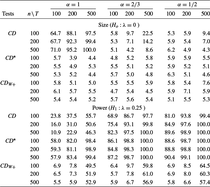
The simulation results for the DGPs with the errors following Gaussian distribution are shown in Tables 1–4. Table 1 gives the test results for the latent factor model with one factor, ( $m_{0}=1$ ). As to be expected, the standard CD test over-rejects when the factor is strong, namely, when $\alpha =1$ . By comparison, the rejection frequencies of both CD $^{\ast }$ and CD $_{W+}$ tests under the null ( $\lambda =0)$ are generally around the nominal size of $5$ %. Under the alternative (when $\lambda =0.25$ ), the CD $^{\ast }$ test has satisfactory power properties with significantly high rejection frequencies even when the sample size is small. But the CD $_{W+}$ test performs quite poorly under the spatial alternative, especially when T is small.

Table 1

Size and power of tests of error cross-sectional dependence using one PC $(\hat {m}=1)$ for the latent factor model with one factor $(m_{0}=1)$ and serially independent Gaussian errors

Table 1 Long description

The table is organized into two primary vertical sections: Size (null hypothesis lambda equals 0) and Power (alternative hypothesis lambda equals 0.25). The columns are grouped by alpha values: alpha equals 1, alpha equals 2 forward slash 3, and alpha equals 1 forward slash 2. Under each alpha, there are sub-columns for sample sizes T equals 100, 200, and 500. The rows are categorized by the test type (C D, C D super asterisk, and C D sub W plus) and further subdivided by sample size n equals 100, 200, and 500.

In the Size section:

- C D shows high values (64.7 to 100.0) when alpha equals 1, but decreases as alpha decreases, though it remains inflated at 22.5 for alpha equals 2 forward slash 3, T equals 500.

- C D super asterisk and C D sub W plus maintain stable size values near the 5 percent nominal level (ranging from 3.9 to 7.6) across all alpha and sample size combinations.

In the Power section:

- C D power decreases as n increases when alpha equals 1 (from 23.8 to 10.9), but increases with n for lower alpha values.

- C D super asterisk shows high power (57.9 to 100.0) across all alpha values, generally increasing with sample size T.

- C D sub W plus shows low power for T equals 100 and 200 (5.5 to 9.7) but a significant jump in power at T equals 500 (49.5 to 64.5).

Note: The DGP is given by (44) with $\beta _{i1}=\beta _{i2}=0$ and contains a single latent factor with different factor strengths, $\alpha =1, 2/3$ , and $1/2$ . $\lambda $ denotes the spatial autocorrelation coefficient defined by (48). $m_{0}$ is the true number of factors and $\hat {m}$ is the number of selected PCs used to compute the different CD statistics. $CD$ denotes the standard test of error cross-sectional dependence defined by (16), $CD^{\ast }$ is the bias-corrected version defined by (31), and $CD_{W+}$ is the power-enhanced randomized version defined by (50).

Table 2

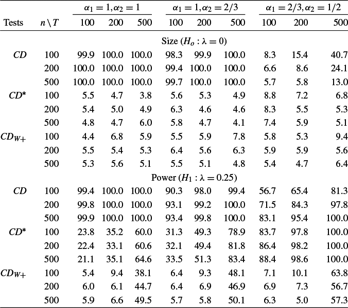
Size and power of tests of error cross-sectional dependence using two PCs $(\hat {m}=2)$ for the latent factor model with two factors $(m_{0}=2)$ and serially independent Gaussian errors

Table 2 Long description

The table is organized into two main vertical sections: Size (H sub o: lambda = 0) and Power (H sub 1: lambda = 0.25).

Header Structure:

* The top row defines three alpha parameter sets: (alpha sub 1 = 1, alpha sub 2 = 1), (alpha sub 1 = 1, alpha sub 2 = 2/3), and (alpha sub 1 = 2/3, alpha sub 2 = 1/2).

* Under each alpha set, columns are divided by sample size T: 100, 200, and 500.

* The leftmost columns identify the test type (L M, C D super *, C D sub W +) and the sample size n: 100, 200, and 500.

Data Summary for Size (H sub o: lambda = 0):

* L M test: Shows high values (98.3 to 100.0) for the first two alpha sets, but lower values (5.7 to 40.7) for the third set.

* C D super * and C D sub W + tests: Maintain values close to the 5 percent nominal level, ranging from 3.8 to 9.4 across all alpha sets and sample sizes.

Data Summary for Power (H sub 1: lambda = 0.25):

* L M test: High power across all sets, generally increasing with T and n, reaching 100.0 in many cases.

* C D super * test: Power increases significantly as alpha values decrease and sample sizes increase, ranging from 21.1 to 100.0.

* C D sub W + test: Shows lower power compared to others, with a notable increase to 63.8 only at the largest sample sizes (n=100, T=500) in the third alpha set.

Note: The DGP is given by (44) with $\beta _{i1}=\beta _{i2}=0$ , and contains two latent factors with different factor strengths, $(\alpha _{1},\alpha _{2})=(1,1)$ , $(1,2/3)$ , and $(2/3,1/2)$ . See also the note to Table 1.

Table 3

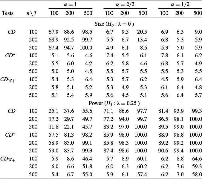
Size and power of tests of error cross-sectional dependence using one PC $(\hat {m}=1)$ for the panel regression model with one latent factor $(m_{0}=1)$ and serially independent Gaussian errors

Table 3 Long description

The table is organized into two main vertical sections: Size (null hypothesis lambda equals 0) and Power (alternative hypothesis lambda equals 0.25).

Horizontal headers define three alpha levels: alpha equals 1, alpha equals 2/3, and alpha equals 1/2. Under each alpha level, sample sizes (n minus T) are listed as 100, 200, and 500.

Vertical headers list three tests: L M, C D super asterisk, and C D sub W plus.

Key data points in the Size section:

* L M test shows high size distortion at alpha equals 1 (67.9 to 100.0) but improves as alpha decreases.

* C D super asterisk and C D sub W plus maintain stable sizes near the 5 percent nominal level across most alpha and sample size combinations, ranging roughly between 4.2 and 7.8.

Key data points in the Power section:

* L M test power increases with sample size, reaching 100.0 at alpha equals 2/3 and 1/2 for larger samples.

* C D super asterisk shows high power (up to 100.0) across all alpha levels as sample size increases.

* C D sub W plus shows significantly lower power compared to the other tests, particularly at smaller sample sizes, with values often below 10.0, only reaching approximately 55.0 to 64.6 at n minus T equals 500.

Note: The DGP is given by (44) with $\beta _{i1}$ and $\beta _{i2}$ both generated from normal distribution, and contains a single latent factor with different factor strengths, $\alpha =1, 2/3$ , and $1/2$ . See also the note to Table 1.

Table 4

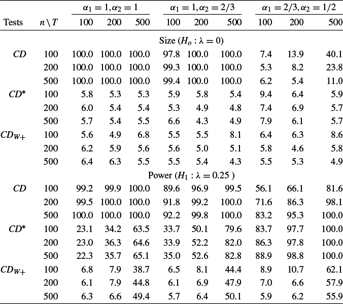
Size and power of tests of error cross-sectional dependence using two PCs $(\hat {m}=2)$ for the panel regression model with two latent factors $(m_{0}=2)$ and serially independent Gaussian errors

Table 4 Long description

The table is structured with three main columns for alpha parameter sets: alpha sub 1 equals 1, alpha sub 2 equals 1; alpha sub 1 equals 1, alpha sub 2 equals 2/3; and alpha sub 1 equals 2/3, alpha sub 2 equals 1/2. Each alpha set is subdivided by sample sizes n and T of 100, 200, and 500. The rows are divided into two primary sections: Size (H sub o: lambda equals 0) and Power (H sub 1: lambda equals 0.25).

Within each section, three tests are evaluated: L M, C D super asterisk, and C D sub W plus.

Key data trends:

* In the Size section, the L M test shows values near 100.0 for the first two alpha sets but drops significantly for the third set (e.g., 7.4 at n, T equals 100). C D super asterisk and C D sub W plus maintain values close to the 5 percent nominal level (ranging from 4.3 to 9.4).

* In the Power section, the L M test shows high power (often 100.0) across most configurations. C D super asterisk power increases with sample size, reaching 100.0 in the third alpha set at n, T equals 500. C D sub W plus shows lower power compared to the other tests, particularly in smaller sample sizes, but improves as n and T increase to 500.

Note: The DGP is given by (44) with $\beta _{i1}$ and $\beta _{i2}$ both generated from normal distribution, and contains two latent factors with different factor strengths, $(\alpha _{1},\alpha _{2})=(1,1),\text { }(1,2/3),\text { and }(2/3,1/2)$ . See also the note to Table 1.

Table 2 summarizes the size and power results for the latent factor model with $m_{0}=2,$ and reports the results when $\hat {m}$ (the selected number of PCs) is set to $2$ . The results are qualitatively similar to the ones reported for the one factor model. The CD test over-rejects if at least one of the factors is strong, but CD $^{\ast }$ and CD $_{W+}$ tests have sizes that are close to their nominal value of $5$ %. In terms of power, the CD $^{\ast }$ test performs well while the power of the CD $_{W^{+}}$ test is now even lower and quite close to $5$ % when $T<500$ .

Turning to panel regression models with latent factors estimated by CCE, the associated simulation results are summarized in Tables 3 and 4. As can be seen, the results are very close to the ones reported in Tables 1 and 2 for the latent factor model, and are in line with the asymptotic result in (39) that underlies the use of the CCE approach to filter out the effects of observed covariates, as well as latent factors.

7.3.2 Serially Independent Errors: Chi-Squared Distributed Errors

To save space, the simulation results for the DGPs with chi-squared errors are provided in Tables S.1–S.4 in the supplement of Pesaran and Xie (Reference Pesaran and Xie2025). For the standard CD test and its biased-corrected version, CD $^{\ast }$ , as shown in Tables S.1 and S.2, the results are very similar to the ones with Gaussian errors, suggesting that the CD $^{\ast}$ test is likely to be robust to departures from Gaussianity. As with the experiments with Gaussian errors, the standard CD test continues to over-reject unless $\alpha <2/3$ , and the CD $^{\ast}$ test has the correct size for all n and T combinations except when $T=100$ . The main difference between the results with and without Gaussian errors is the tendency for the CD $_{W^{+}}$ test to over-reject when $n>T$ , which seems to be a universal feature of this test and holds for all choices of $m_{0}$ , irrespective of whether the factors are strong or weak. This could be due to the screening component of the CD $_{W+}$ test not tending to zero sufficiently fast with n and T. Furthermore, the CD $^{\ast}$ test continues to have satisfactory power, but the CD $_{W^{+}}$ test clearly lacks power against spatial or network alternatives that are of primary interest.

Similar results are obtained for panel regression models with latent factors, summarized in Tables S.3 and S.4 in the supplement of Pesaran and Xie (Reference Pesaran and Xie2025).

7.3.3 Serially Correlated Errors

To save space, the results for the DGPs with serially correlated errors are summarized in Tables S.5–S.20 in the supplement of Pesaran and Xie (Reference Pesaran and Xie2025). Tables S.5–S.12 give the simulation results for the variance-adjusted CD tests, while Tables S.13–S.20 provide the results for the ARDL-adjusted tests. Overall, the results corroborate our earlier findings obtained for DGPs with serially independent errors. Both adjustments for serial error correlation work well, with size and power of the adjusted CD $^{\ast}$ tests being quite close to the results already reported for DGPs with serially independent errors. It is also clear that without adjustments for latent factors and error serial correlation, the standard CD test will lead to large size distortions when the latent factors are strong. But in line with our theoretical results, the standard CD test, when adjusted for error serial correlation if needed, tends to have the correct size when the latent factors are weak.

Comparing the two types of adjustments for error serial correlations (for pure latent factor models as well as for panel regression models with latent factors), the variance-adjusted CD $^{\ast}$ test works particularly well, and only shows mild over-rejection in the case where $T=100$ and $n>T$ . In contrast, the CD $_{W+}$ test with variance adjustment over-rejects for all combinations of n and T.

The ARDL-adjusted version of the CD $^{\ast}$ test also works well and tends to have the correct size for all $(n,T)$ combinations, although we observe some slight over-rejection when $n=100$ . The CD $_{W+}$ test using ARDL adjustment does better in controlling for the size when the errors are Gaussian, but tends to over-reject when the errors are chi-squared distributed and $n>T$ . Both adjusted versions of the CD $_{W+}$ test continue to lack power against spatial or network alternatives.

8 EMPIRICAL APPLICATION

It is well known that house price changes are spatially correlated, but it is unclear if such correlations are mainly due to common factors (national or regional) or arise from spatial spillover effects not related to the common factors, a phenomenon also referred to as the ripple effect (see, for example, (Holly, Pesaran, and Yamagata, Reference Holly, Pesaran and Yamagata2011; Tsai, Reference Tsai2015; Bailey et al., Reference Bailey, Holly and Pesaran2016; Chiang and Tsai, Reference Chiang and Tsai2016; Aquaro et al., Reference Aquaro, Bailey and Pesaran2021)). To test for the presence of ripple effects, the influence of common factors must first be filtered out and this is often a challenging exercise due to the latent nature of regional and national factors. Therefore, to find if there exist local spillover effects, one needs to test for significant residual cross-sectional dependence once the effects of common factors are filtered out.

We consider quarterly data on real house prices at the level of Metropolitan Statistical Areas (MSAs) in the United States. There are 381 MSAs, under the February 2013 definition provided by the U.S. Office of Management and Budget (OMB). We use quarterly data on real house price changes compiled by Yang (Reference Yang2021) which covers $n=377$ MSAs from the contiguous United States over the period 1975Q1–2014Q4 ( $T=160$ quarters). To allow for possible regional factors, we also follow Bailey et al. (Reference Bailey, Holly and Pesaran2016) and start with the Bureau of Economic Analysis eight regional classification, namely, New England, Mideast, Great Lakes, Plains, Southeast, Southwest, Rocky Mountain, and Far West. But due to the low number of MSAs in New England and Rocky Mountain regions, we combine New England and Mideast, and Southwest and Rocky Mountain as two regions. We end up with a six-region classification ( $R=6$ ), each covering a reasonable number of MSAs.

We model house price changes and consider an extended factor model with deterministic seasonal dummies to allow for seasonal movements in house prices. Bailey et al. (Reference Bailey, Holly and Pesaran2016) find evidence of regional factors in U.S. house price changes, which might not be picked up when using PCA. Given this finding, our model includes observed regional and national factors, as well as latent factors. Specifically, we suppose

(54) $$ \begin{align} \pi_{irt}=a_{ir}+\sum_{j=1}^{3}\beta_{ir,j}\text{l}\left\{ q_{t}=j\right\} +\delta_{ir,1}\bar{\pi}_{rt}+\delta_{ir,2}\bar{\pi}_{t}+\boldsymbol{\gamma }_{ir}^{{\prime}}\mathbf{f}_{t}+u_{irt}, \end{align} $$

where $\pi _{irt}$ is the real house price change in MSA i located in region $r=1,2,\ldots,R$ , l $\left \{ q_{t}=j\right \} $ is the index for quarter j, and $\mathbf {f}_{t}$ is the $m_{0}\times 1$ vector of latent factors. $\bar {\pi }_{rt}=n_{r}^{-1}\sum _{i=1}^{n_{r}}\pi _{irt}$ , where $n=\sum_{r=1}^Rn_r$ , and $n_r$ is the number of MSAs in region $r$ , and $\bar {\pi }_{t}=n^{-1} \sum _{r=1}^{R}\sum _{i=1}^{n_{r}}\pi _{irt}$ are proxies for the regional and national factors. To filter out the effects of seasonal dummies as well as observed factors, we first run the least squares regression of $\pi _{irt}$ on an intercept and $\left ( \text {l}\left \{ q_{t}=j\right \} ,\bar {\pi } _{rt},\bar {\pi }_{t}\right ) $ for each i to generate the residuals

(55) $$ \begin{align} \hat{v}_{irt}=\pi_{irt}-\hat{a}_{ir}-\sum_{j=1}^{3}\hat{\beta}_{ir,j} \text{l}\left\{ q_{t}=j\right\} -\hat{\delta}_{ir,1}\bar{\pi}_{rt} -\hat{\delta}_{ir,2}\bar{\pi}_{t}, \end{align} $$

and then apply PCA to $\left \{ \hat {v}_{irt}:i=1,2,\ldots,n_r,r=1,2,\ldots,R,t=1,2,\ldots,T \right\} $ to obtain $\boldsymbol {\hat {\gamma }}_{ir}$ and $\hat {\mathbf {f}}_{t}$ , yielding the residuals

(56) $$ \begin{align} \hat{u}_{irt}=\pi_{irt}-\hat{a}_{ir}-\sum_{j=1}^{3}\hat{\beta}_{ir,j} \text{l}\left\{ q_{t}=j\right\} -\hat{\delta}_{ir,1}\bar{\pi}_{rt} -\hat{\delta}_{ir,2}\bar{\pi}_{t}-\boldsymbol{\hat{\gamma}}_{ir}^{{\prime} }\hat{\mathbf{f}}_{t}. \end{align} $$

For the case without adjusting for error serial correlation, the above residuals are used to compute $CD$ , $CD^{\ast }$ , and $CD_{W+}$ , given by (16), (31), and (50). For the case with serially correlated errors, the variance-adjusted versions of the three CD statistics are generated by scaling original test statistics using (41), where $\tilde {\varepsilon }_{it,T}$ is replaced by the standardized residuals generated from (56), while the ARDL-adjusted versions are computed using the residuals from the following dynamic panel data model with latent factors, $\mathbf {h}_{t}$ :

(57) $$ \begin{align} \pi_{irt} & =a_{ir}+\rho_{ir}\pi_{irt-1}+\sum_{j=1}^{3}\beta_{ir,j} \text{l}\left\{ q_{t}=j\right\} +\delta_{ir,1}\bar{\pi}_{rt}+\delta _{ir,2}\bar{\pi}_{t}\nonumber\\ &\quad +\sum_{j=1}^{3}\lambda_{ir,j}\text{l}\left\{ q_{t-1}=j\right\} +\omega_{ir,1}\bar{\pi}_{rt-1}+\omega_{ir,2}\bar{\pi}_{t-1}+\mathbf{g} _{ir}^{\prime}\mathbf{h}_{t}+\epsilon_{irt}. \end{align} $$

To estimate the number of latent factors, m, we consider the information criteria $IC_{P1}$ and $IC_{P2}$ proposed by Bai and Ng (Reference Bai and Ng2002), and the $ER$ and $GR$ criteria proposed by Ahn and Horenstein (Reference Ahn and Horenstein2013). Given the spatial diversity of U.S. housing market, we set $m_{\max }= 10$ , although once we allow for national and regional factors, we would expect $m_{0}$ and its estimate, $\hat {m}$ , to be relatively small. The estimated number of factors and the associated CD test statistics are summarized in Table 5. The first four columns of the table report $\hat {m}$ , $CD$ , $CD^{\ast }$ , and $CD_{W+}$ statistics that are not adjusted for error serial correlation, while the middle and the final four columns report the variance-adjusted and ARDL-adjusted versions of these statistics, respectively.

Table 5

Tests of error cross-sectional dependence for the house price application

Table 5 Long description

The table is organized into three main horizontal sections under the primary header.

1. Not adjusted for error serial correlation:

- I C sub p 1: m-hat 10, C D 22.2, C D super star 53.8, C D sub W plus 1,080.9.

- I C sub p 2: m-hat 4, C D 112.4, C D super star 122.4, C D sub W plus 1,444.8.

- E R: m-hat 2, C D 107.9, C D super star 117.9, C D sub W plus 1,588.4.

- G R: m-hat 2, C D 107.9, C D super star 117.9, C D sub W plus 1,588.4.

2. Adjusted for error serial correlation (Variance adjusted):

- I C sub p 1: m-hat 10, C D 10.5, C D super star 25.5, C D sub W plus 512.2.

- I C sub p 2: m-hat 4, C D 50.7, C D super star 55.3, C D sub W plus 652.3.

- E R: m-hat 2, C D 47.3, C D super star 51.8, C D sub W plus 697.1.

- G R: m-hat 2, C D 47.3, C D super star 51.8, C D sub W plus 697.1.

3. Adjusted for error serial correlation (A R D L adjusted):

- I C sub p 1: m-hat 10, C D 59.1, C D super star 64.7, C D sub W plus 1,171.9.

- I C sub p 2: m-hat 2, C D 64.7, C D super star 66.3, C D sub W plus 1,598.4.

- E R: m-hat 1, C D 60.3, C D super star 61.4, C D sub W plus 1,766.8.

- G R: m-hat 1, C D 60.3, C D super star 61.4, C D sub W plus 1,766.8.

Note: The test statistics that do not adjust for serial correlation and that use variance adjustment are based on the panel regression in (54). The test statistics that use ARDL adjustment are based on the panel regression in (57). Both panel regressions allow for seasonal dummies and national and regional effects. $IC_{p1}$ and $IC_{p2}$ denote the two information criteria by Bai and Ng (Reference Bai and Ng2002), while $ER$ and $GR$ refer to the two criteria proposed by Ahn and Horenstein (Reference Ahn and Horenstein2013). The maximum number of latent factors, $m_{\max }$ , is set as $10$ . The number of selected factors is denoted by $\hat {m}$ . $CD$ denotes the standard test of error cross-sectional dependence defined by (16), $CD^{\ast }$ is the bias-corrected version defined by (31), and $CD_{W+}$ is the power-enhanced randomized version defined by (50).

As can be seen in the case of no error serial correlations, there are large differences in the number of factors selected by the different criteria, with $IC_{p1}$ selecting the assumed maximum number of factors, $IC_{p2}$ selecting $4$ , and $ER$ and $GR$ both selecting $2$ factors. These estimates are not affected when we allow for error serial correlations and consider variance adjustment.

CD, CD $^{\ast }$ , and CD $_{W+}$ tests all reject the null hypothesis of cross-sectional independence, irrespective of the choices of $\hat {m}$ and whether we allow for error serial correlation. In view of the theoretical and finite sample results reported in this article, it is advisable to focus on the CD $^{\ast}$ test results and recognize that the relatively large magnitudes obtained for CD and CD $_{W+}$ test statistics could be due to their tendencies to over-rejection in the presence of strong latent factors and non-Gaussian errors. Focusing on $CD^{\ast }$ , we find that even with $\hat {m}=10,$ the CD $^{\ast}$ test strongly rejects the null of cross-sectional independence with $CD^{\ast }$ statistic of $25.5$ , compared to 95% critical value of $1.96$ . There is clear evidence that in addition to latent factors, spatial modeling of the type carried out in Bailey et al. (Reference Bailey, Holly and Pesaran2016) and Aquaro et al. (Reference Aquaro, Bailey and Pesaran2021) is likely to be necessary to account for the remaining error cross-sectional dependence.

9 CONCLUDING REMARKS

This article revisits the problem of testing error cross-sectional independence in panel data models with latent factors. Starting with a pure latent multifactor model, we show that the standard CD test proposed by Pesaran (Reference Pesaran2004) remains valid if the latent factors are weak, but over-reject when one or more of the latent factors are strong. The over-rejection of the CD test in the case of strong factors is also established by Juodis and Reese (Reference Juodis and Reese2022), who propose a randomized test statistic to correct for over-rejection and add a screening component to achieve power. However, as we show, JR’s CD $_{W^{+}}$ test is not guaranteed to have the correct size and need not be powerful against spatial or network alternatives. Such alternatives are of particular interest in the analyses of ripple effects in housing markets, and clustering of firms within industries in capital or arbitrage asset pricing models. In fact, using Monte Carlo experiments, we show that under non-Gaussian errors, the JR test continues to over-reject when the cross section dimension (n) is larger than the time dimension (T), and often has power close to size against spatial alternatives. To overcome some of these shortcomings, we propose a simple bias-corrected CD test statistic, labeled $CD^{\ast }$ , which is shown to be asymptotically $\mathcal {N}(0,1)$ under the null when n and $T\rightarrow \infty $ such that $n/T\rightarrow \kappa $ , for a fixed constant $\kappa $ . In addition, the CD $^{\ast}$ test is shown to have power against network-type dependence. These results hold for pure latent factor models as well as for panel regression models with latent factors. To deal with possible error serial dependence, following Baltagi et al. (Reference Baltagi, Kao and Peng2016), we also consider a variance-adjusted version of $CD^{\ast }$ , as well as an alternative ARDL-adjusted version that eliminates the error serial dependence before the application of the CD $^{\ast}$ test procedure. Both of these approaches are shown to perform well within the Monte Carlo setup of the article.