





1. Introduction
It is well known that vortex-sheet evolution is ill posed and develops a curvature singularity in finite time due to the Kelvin–Helmholtz (K–H) instability (Moore Reference Moore1979; Caflisch & Orellana Reference Caflisch and Orellana1986, Reference Caflisch and Orellana1989; Krasny Reference Krasny1986b ; Caflisch et al. Reference Caflisch, Orellana and Siegel1990; Pullin & Shen Reference Pullin and Shen2023). Regularisations by using vortex blobs (Krasny Reference Krasny1986a ), vortex layers (Baker & Shelley Reference Baker and Shelley1990) and surface tension (Hou et al. Reference Hou, Lowengrub and Shelley1994, Reference Hou, Lowengrub and Shelley1997) have been shown to mitigate or cut off the high-wavenumber K–H instability and remove the curvature singularity. However, there still exist unstable eigenmodes which can cause the interface to roll up. On the other hand, it is known that a tangential electric field (TEF) can stabilise fluid systems in various physical scenarios (Melcher & Schwarz Jr. Reference Melcher and Schwarz1968; Tilley et al. Reference Tilley, Petropoulos and Papageorgiou2001; Papageorgiou Reference Papageorgiou2019). The Rayleigh–Taylor instability can be suppressed by a sufficiently strong TEF, as shown by weakly nonlinear models (Barannyk et al. Reference Barannyk, Papageorgiou and Petropoulos2012, Reference Barannyk, Papageorgiou, Petropoulos and Vanden-Broeck2015) and direct numerical simulations of the Navier–Stokes equations (Cimpeanu et al. Reference Cimpeanu, Papageorgiou and Petropoulos2014; Yang et al. Reference Yang, Li, Zhao, Shao and Xu2016; Anderson et al. Reference Anderson, Cimpeanu, Papageorgiou and Petropoulos2017). Linear stability analysis shows that a strong TEF can suppress the K–H instability for all wavenumbers, thus distinguishing it from the other regularisations mentioned above. Grandison et al. (Reference Grandison, Papageorgiou and Vanden-Broeck2012) showed that coupling TEFs with surface tension can suppress rupture of planar jets. These studies motivate the current investigation on the electrified vortex-sheet problem, given the surmise that the vortex sheet could become well posed and the curvature singularity eliminated. However, there exists limited numerical evidence that suggests that the latter may not be true. Kochurin & Zubarev (Reference Kochurin and Zubarev2018) and Kochurin (Reference Kochurin2019a ,Reference Kochurin b ) found curvature singularities in surface gravity-capillary waves even when there is a strong TEF. A reasonable explanation is that a sufficiently strong TEF makes the system almost non-dispersive. Therefore, for small-amplitude perturbations, the leading-order asymptotic model should be a quadratic nonlinear equation without linear dispersive terms, which is likely to develop a shock in finite time. To our knowledge, the regularity of electrified vortex sheets and their evolution is an open question. Of interest also is the recent study by Sohn & Baek (Reference Sohn and Baek2026) who address electrified vortex-sheet evolution by incorporating a vortex blob regularisation; hence, there is little overlap with our study which is entirely focussed on singularity formation and how it is affected by the electric field.
We consider vortex sheets between two dielectric, incompressible and inviscid fluids subjected to a uniform TEF. Given small-amplitude initial perturbations, we study their temporal evolution. To derive weakly nonlinear models, we take advantage of the Hamiltonian structure supported by the electrified vortex-sheet system. The Hamiltonian formulation was introduced to water waves by the pioneering work of Zakharov (Reference Zakharov1968). Later, Benjamin & Bridges (Reference Benjamin and Bridges1997) extended this formulation to two-layer interfacial flows with a uniform background shear, i.e. the vortex-sheet problem. Recently, the Hamiltonian approach has been widely applied to studies of electrified surface and interfacial waves (Kochurin et al. Reference Kochurin, Zubarev and Zubareva2013; Kochurin & Zubarev Reference Kochurin and Zubarev2018; Wang Reference Wang2017; Kochurin Reference Kochurin2019a , Reference Kochurinb ; Guan & Wang Reference Guan and Wang2022; Wang Reference Wang2022; Sohn & Baek Reference Sohn and Baek2026). In particular, Wang (Reference Wang2022) showed that the Hamiltonian of electrified two-layer shear-free potential flows is the Benjamin–Bridges Hamiltonian but incorporating the perturbed electric potential energy. By taking a variational derivative, the electric-energy term gives rise to the Maxwell stress tensor and leads to the correct dynamic boundary conditions. Combining the results of Benjamin & Bridges (Reference Benjamin and Bridges1997) and Wang (Reference Wang2022), it is trivial to extend the Hamiltonian formulation to our current problem. The superiority of the Hamiltonian approach comes from the fact that the global dependence of the unknowns, i.e. the Birkhoff–Rott equation and its equivalent integral relations, is intrinsically built into the Dirichlet–Neumann operators (DNOs), which can be asymptotically truncated to arbitrary orders through the Craig–Sulem recursion relation (Craig & Sulem Reference Craig and Sulem1993). This property has been widely used to derive weakly nonlinear models in various physical scenarios (Craig & Groves Reference Craig and Groves1994; Craig et al. Reference Craig, Guyenne and Sulem2012; Wang & Milewski Reference Wang and Milewski2012; Wang Reference Wang2017; Guan & Wang Reference Guan and Wang2022; Xu & Wang Reference Xu and Wang2025; Feng & Yang Reference Feng and Yang2026).
For fully nonlinear simulations of vortex sheets, the most efficient approach is the boundary integral method (BIM). In two dimensions there are three often-used versions: by using the Birkhoff–Rott equation (Baker et al. Reference Baker, Meiron and Orszag1982; Hou et al. Reference Hou, Lowengrub and Shelley1994, Reference Hou, Lowengrub and Shelley1997; Baker & Nachbin Reference Baker and Nachbin1998; Ambrose et al. Reference Ambrose, Camassa, Marzuola, McLaughlin, Robinson and Wilkening2022); using a Green’s function to derive a boundary integral equation (Longuet-Higgins & Cokelet Reference Longuet-Higgins and Cokelet1976; Baker et al. Reference Baker, Meiron and Orszag1982; Yang Reference Yang1992); and deriving the boundary integral equation by using Cauchy’s integral formula (Dold & Peregrine Reference Dold and Peregrine1986; Dold Reference Dold1992; Grue et al. Reference Grue, Friis, Palm and Rusaas1997; Ambrose et al. Reference Ambrose, Camassa, Marzuola, McLaughlin, Robinson and Wilkening2022; Guan & Vanden-Broeck Reference Guan and Vanden-Broeck2025). In this paper, we adopt the latter approach. Owing to the irrotationality and incompressibility of the flow field and the harmonic nature of the electrostatic field, one can introduce two related analytic functions that satisfy Cauchy’s integral formula at the interface. The resulting boundary integral equations take the form of Fredholm integral equations of the second kind, enabling efficient implementation of iterative solvers such as the generalised minimum residual method (GMRES). To track the evolution of the interface, we employ the
 $\theta -s_\alpha$
formulation (Yang Reference Yang1992; Hou et al. Reference Hou, Lowengrub and Shelley1994; Guan & Vanden-Broeck Reference Guan and Vanden-Broeck2025), which uses the tangent angle and the arclength derivative along the interface as primary unknowns. This removes the restriction that the interface must be a graph of the horizontal variable, allowing us to simulate overturned interfaces as long as there is no topological change. The formulation can be embedded into an Eulerian framework where all grid points are evenly separated using arclength as a parameter (Yang Reference Yang1992; Hou et al. Reference Hou, Lowengrub and Shelley1994; Guan & Vanden-Broeck Reference Guan and Vanden-Broeck2025). By using the small-scale decomposition method (Hou et al. Reference Hou, Lowengrub and Shelley1994, Reference Hou, Lowengrub and Shelley1997) (essentially an integrating-factor technique), we can significantly eliminate the capillary-induced numerical stiffness. In the current paper, there is no severe numerical-stiffness issue because we do not consider surface tension. In contrast, we find that the Lagrangian approach provides superior computational accuracy because fluid markers can cluster in the region where the curvature singularity develops.
The rest of the paper is organised as follows. Section 2 describes the problem setting, mathematical formulation, non-dimensionalisation and linear dispersion relation. Section 3 illustrates the Hamiltonian formulation, expansions of the DNOs and derives various weakly nonlinear models, a special case of which is a novel evolution equation for classical vortex sheets. Section 4 demonstrates the BIM
 $\theta -s_\alpha$
formulation, and includes details of the fully nonlinear simulations. Section 5 reports numerical results of the BIM and compares them with solutions of the models. Section 6 provides our conclusions.
2. Governing equations
We consider an electrified vortex sheet between two immiscible ideal fluids with a uniform TEF of strength
 $E_0$
acting parallel to the initially flat interface. Inside each fluid, there is a constant background flow
 $\tilde {U}_{\!j}$
, where the subscript
 $j$
is used to denote the lower fluid when
 $j=1$
, and the upper fluid when
 $j=2$
. The fluids are assumed to be perfect dielectrics with constant permittivities
 $\varepsilon _{\!j}$
and constant densities
 $\rho _{\!j}$
. We use
 $x$
and
 $y$
to denote the usual horizontal and vertical Cartesian coordinates. For convenience, the
 $y$
-axis points upwards and the
 $x$
-axis points in the direction of the electric field and coincides with the undisturbed interface. A schematic is given in figure 1. If at some given time
 $t$
the interface has elevation
 $\eta (x,t)$
, our objective is to calculate the subsequent evolution of the interface and in particular investigate whether an initially smooth interface remains smooth at later times.
Schematic of the electrified vortex sheet.

Assuming the flows are irrotational, we can introduce two perturbed velocity potentials
 $\phi _{\!j}$
so that the velocity
 $\boldsymbol{u}_{\!j}$
in each layer can be written as
 \begin{align} \boldsymbol{u}_{\!j} = \tilde {U}_{\!j}{\boldsymbol {i}}+\boldsymbol{\nabla }\phi _{\!j},\quad \text{for} \quad j = 1 \quad \text{and}\quad 2, \end{align}
where
 $\boldsymbol {i}$
denotes the unit vector in the
 $x$
-direction, and
 $\boldsymbol{\nabla }= (\partial _x,\partial _y)$
. Similarly, the electrostatic limit of Maxwell’s equations allows us to introduce perturbed voltage potentials
 $V_1$
and
 $V_2$
so that the electric field can be expressed as
 \begin{align} \boldsymbol{E}_{\!j} = E_0{\boldsymbol {i}} + \boldsymbol{\nabla }V_{\!j}, \quad \text{for} \quad j = 1 \quad \text{and} \quad 2. \end{align}
The velocity and voltage potentials satisfy Laplace’s equation
 \begin{align} \begin{cases} \phi _{1,xx} + \phi _{1,yy} = 0, \quad &\text{for} \,\,\, -\infty \lt y\lt \eta (x,t),\\[3pt] V_{1,xx} + V_{1,yy} = 0, \quad &\text{for} \,\,\, -\infty \lt y\lt \eta (x,t),\\[3pt] \phi _{2,xx} + \phi _{2,yy} = 0, \quad &\text{for} \,\,\,\eta (x,t)\lt y\lt \infty ,\\[3pt] V_{2,xx} + V_{2,yy} = 0, \quad &\text{for} \,\,\,\eta (x,t)\lt y\lt \infty . \end{cases} \end{align}
At the interface
 $y = \eta (x,t)$
, we have two kinematic boundary conditions
 \begin{align} \begin{cases} \eta _t + (\tilde {U}_1+\phi _{1,x})\eta _x = \phi _{1,y},\\[3pt] \eta _t + (\tilde {U}_2+\phi _{2,x})\eta _x = \phi _{2,y}, \end{cases} \end{align}
and a dynamic boundary condition
 \begin{align} \rho _1\bigg (\phi _{1,t} + \frac 12 |\boldsymbol{u_1}|^2 + g\eta \bigg ) - \rho _2\bigg (\phi _{2,t} + \frac 12 |\boldsymbol{u_2}|^2 + g\eta \bigg ) + \big [\boldsymbol{n}\boldsymbol{\cdot }\boldsymbol{\varSigma }\boldsymbol{\cdot }\boldsymbol{n}\big ]_2^1 = 0, \end{align}
where
 $\boldsymbol{n} = (-\eta _x,1)/\sqrt {1+\eta _x^2}$
is the unit normal vector pointing into fluid 2, and
 $\boldsymbol{\varSigma }$
represents the Maxwell stress tensor
 \begin{align} \boldsymbol{\varSigma } = \varepsilon _{\!j} \boldsymbol{E}_{\!j}\otimes \boldsymbol{E}_{\!j} - \frac {\varepsilon _{\!j}}{2}\,|\boldsymbol{E}_{\!j}|^2\,I \quad \,\,\, \text{in fluid } j. \end{align}
After some algebra we can write
 \begin{align} \big [\boldsymbol{n}\boldsymbol{\cdot }\boldsymbol{\varSigma }\boldsymbol{\cdot }\boldsymbol{n}\big ]_2^1 = \frac {\varepsilon _1}{2}\Big [\big (\boldsymbol{E}_1\boldsymbol{\cdot }\boldsymbol{n}\big )^2-\big (\boldsymbol{E}_1\boldsymbol{\cdot }\boldsymbol{t}\big )^2\Big ] - \frac {\varepsilon _2}{2}\Big [\big (\boldsymbol{E}_2\boldsymbol{\cdot }\boldsymbol{n}\big )^2-\big (\boldsymbol{E}_2\boldsymbol{\cdot }\boldsymbol{t}\big )^2\Big ], \end{align}
where
 $\boldsymbol{t} = (1,\eta _x)/\sqrt {1+\eta _x^2}$
is the unit tangent vector along the interface. In addition
 \begin{align} \boldsymbol{E}_{\!j}\boldsymbol{\cdot }\boldsymbol{n} = \frac {\partial V_{\!j}}{\partial \boldsymbol{n}} - E_0\frac {\eta _x}{\sqrt {1+\eta _x^2}}, \quad \boldsymbol{E}_{\!j}\boldsymbol{\cdot }\boldsymbol{t} = \frac {\partial V_{\!j}}{\partial \boldsymbol{t}} + E_0\frac {1}{\sqrt {1+\eta _x^2}}. \end{align}
The notation
 ${\partial V_{\!j}}/{\partial \boldsymbol{n}}=\boldsymbol{\nabla }V_{\!j}\boldsymbol{\cdot }\boldsymbol{n}$
and
 ${\partial V_{i}}/{\partial \boldsymbol{t}}=\boldsymbol{\nabla }V_{\!j}\boldsymbol{\cdot }\boldsymbol{t}$
has been introduced in (2.8), and will be used in the remainder of the paper. Furthermore, we have two boundary conditions at
 $y = \eta (x,t)$
for the voltage potentials. Namely, continuity of voltage potentials
 \begin{align} V_1 = V_2, \end{align}
and continuity of the electric displacement field
 \begin{align} \varepsilon _1 \boldsymbol{E_1}\boldsymbol{\cdot }\boldsymbol{n} - \varepsilon _2 \boldsymbol{E_1}\boldsymbol{\cdot }\boldsymbol{n} = 0\quad \Rightarrow \quad \varepsilon _1 \frac {\partial V_1}{\partial \boldsymbol{n}} - \varepsilon _2 \frac {\partial V_2}{\partial \boldsymbol{n}} = E_0(\varepsilon _1-\varepsilon _2)\frac {\eta _x}{\sqrt {1+\eta _x^2}}. \end{align}
Finally, we impose far-field conditions as
 $|y|\rightarrow \infty$
 \begin{align} \phi _{\!j} \rightarrow 0, \quad V_{\!j} \rightarrow 0 \quad \text{for} \quad j = 1 \quad \text{and} \quad 2. \end{align}
Without loss of generality we assume that
 $\tilde {U}_1 = -\tilde {U}_2 = \tilde {U}/2$
(a Galilean transformation can always achieve this). The system is non-dimensionalised by choosing typical scales for length, time, velocity, density, permittivity and electric field strength as
 \begin{align} \frac {L}{2\pi }, \quad \frac {L}{2\pi |\tilde U|}, \quad |\tilde {U}|, \quad \rho _1, \quad \varepsilon _1, \quad E_0, \end{align}
where
 $L$
is the smallest spatial period of the initial periodic perturbation. The following dimensionless parameters emerge:
 \begin{align} R = \frac {\rho _2}{\rho _1}, \quad F_r = \frac {|\tilde U|}{\sqrt {gL}}, \quad \varepsilon = \frac {\varepsilon _2}{\varepsilon _1}, \quad E_b = \frac {E_0^2 \varepsilon _1}{\rho _1 \tilde {U}^2}, \end{align}
which denote the density ratio, the Froude number for the flow, the permittivity ratio and an electric Weber number that measures the strength of the imposed electric field. The dimensionless kinematic and dynamic boundary conditions now read
 \begin{equation} \begin{cases} \eta _t + \dfrac {U}{2}\eta _x + \phi _{1,x}\eta _x = \phi _{1,y},\\[9pt] \eta _t - \dfrac {U}{2}\eta _x + \phi _{2,x}\eta _x = \phi _{2,y},\\[9pt] \phi _{1,t} - R \phi _{2,t} + \dfrac {U}{2}(\phi _{1,x}+ R\phi _{2,x}) + \dfrac {|\boldsymbol{\nabla }{\phi _1}|^2}{2} - \dfrac {R|\boldsymbol{\nabla }\phi _2|^2}{2} + \dfrac {(1-R)\eta }{F_r^2} + \dfrac {E_b}{2}\big [\boldsymbol{n}\boldsymbol{\cdot }\boldsymbol{\varSigma }\boldsymbol{\cdot }\boldsymbol{n}\big ]_2^1 = 0, \end{cases} \end{equation}
where the dimensionless background shear
 $U$
takes the values
 $1$
or
 $-1$
. The normal Maxwell shear stress (2.7) becomes
 \begin{align} \big [\boldsymbol{n}\boldsymbol{\cdot }\boldsymbol{\varSigma }\boldsymbol{\cdot }\boldsymbol{n}\big ]_2^1 &= \bigg [\frac {\partial V_1}{\partial \boldsymbol{n}}-\frac {\eta _x}{\sqrt {1+\eta _x^2}}\bigg ]^2 - \bigg [\frac {\partial V_1}{\partial \boldsymbol{t}}+\frac {1}{\sqrt {1+\eta _x^2}}\bigg ]^2 \nonumber \\[3pt] &- \varepsilon \bigg [\frac {\partial V_2}{\partial \boldsymbol{n}}-\frac {\eta _x}{\sqrt {1+\eta _x^2}}\bigg ]^2 + \varepsilon \bigg [\frac {\partial V_2}{\partial \boldsymbol{t}}+\frac {1}{\sqrt {1+\eta _x^2}}\bigg ]^2, \end{align}
while the boundary conditions (2.9) and (2.10) become
 \begin{align} \begin{cases} V_1 = V_2,\\[7pt] \dfrac {\partial V_1}{\partial \boldsymbol{n}} - \varepsilon \dfrac {\partial V_2}{\partial \boldsymbol{n}} = (1-\varepsilon )\dfrac {\eta _x}{\sqrt {1+\eta _x^2}} .\end{cases} \end{align}
Solving the linearised system by looking for solutions proportional to
 $\mathrm e^{ i(kx-\omega t)}$
(see Appendix A, where we also include a physical discussion of the stabilising electrostatic mechanism), one can derive two branches for the dispersion relation, namely
 \begin{align} \omega = \frac {U(1-R)}{2(1+R)}k \pm \sqrt {\frac {1-R}{(1+R)F_r^2}|k| + \frac {E_b(1-\varepsilon )^2}{(1+\varepsilon )(1+R)}k^2 - \frac {R}{(1+R)^2}k^2}. \end{align}
The three terms inside the square root represent, from left to right, the effects of buoyancy, the TEF and the background shear, respectively. When
 $R\leqslant 1$
(i.e. the heavier fluid is below), the system is neutrally stable for sufficiently strong fields satisfying
 \begin{align} E_b \gt \frac {R (1+\varepsilon )}{(1+R)(1-\varepsilon )^2}. \end{align}
Otherwise, it is linearly unstable due to the K–H instability. Note also that if Rayleigh–Taylor instability enters when
 $R\gt 1$
, then the flow will be linearly unstable for long enough waves (small enough
 $k$
) irrespective of the value of
 $E_b$
. The interplay between Rayleigh–Taylor instability and the electric field has been considered for both inviscid and viscous flows (Barannyk et al. Reference Barannyk, Papageorgiou and Petropoulos2012, Reference Barannyk, Papageorgiou, Petropoulos and Vanden-Broeck2015; Cimpeanu et al. Reference Cimpeanu, Papageorgiou and Petropoulos2014; Yang et al. Reference Yang, Li, Zhao, Shao and Xu2016; Guo et al. Reference Guo, Zhang and He2023).
Physically, the insulating perfect dielectric fluids modelled here will support polarisation charges on the interface. Following Jackson (Reference Jackson2012, pp. 108–112), the polarisation-charge density is given by
 \begin{align} \sigma _p = (\boldsymbol{P}_1-\boldsymbol{P}_2)\boldsymbol{\cdot }\boldsymbol{n}, \end{align}
where
 $\boldsymbol{P}_{1,2}$
are polarisations defined by (in dimensional form)
 \begin{align} \boldsymbol{P}_{1,2} = \frac {1}{4\pi }\bigg (\frac {\varepsilon _{1,2}}{\varepsilon _0}-1\bigg )\boldsymbol{E}_{1,2}, \end{align}
with
 $\varepsilon _0$
being the electric permittivity of free space. After simplification, we have
 \begin{align} \sigma _p = \frac {\varepsilon _1 \boldsymbol{E_1\boldsymbol{\cdot }\boldsymbol{n}} - \varepsilon _2 \boldsymbol{E_2\boldsymbol{\cdot }\boldsymbol{n}}}{4\pi \varepsilon _0} + \frac {\boldsymbol{E_1\boldsymbol{\cdot }\boldsymbol{n}} - \boldsymbol{E_2\boldsymbol{\cdot }\boldsymbol{n}}}{4\pi }. \end{align}
Using (2.8) and (2.10) gives the desired polarisation-charge distribution on the sheet
 \begin{align} \sigma _p = \frac {1}{4\pi }\bigg ( \frac {\partial V_1}{\partial \boldsymbol{n}} - \frac {\partial V_2}{\partial \boldsymbol{n}} \bigg ). \end{align}
3. Weakly nonlinear models
Zakharov (Reference Zakharov1968) first demonstrated that the water-wave problem under incompressible, irrotational and inviscid assumptions has a Hamiltonian structure. Later, Benjamin & Bridges (Reference Benjamin and Bridges1997) extended the Hamiltonian formulation to two-layer potential flows with a uniform background shear at the interface. They showed that the Hamiltonian is the perturbed energy of the system, and the two canonical variables are the interface elevation
 $\eta$
and the combination of the two perturbed velocity potentials
 $\varphi = \varphi _1 - R\varphi _2$
, where
 $\varphi _1 = \phi _1(x,\eta ,t)$
and
 $\varphi _2 = \phi _2(x,\eta ,t)$
. More recently, the Hamiltonian approach has been widely applied to studies of electrified surface and interfacial waves (Kochurin et al. Reference Kochurin, Zubarev and Zubareva2013; Kochurin & Zubarev Reference Kochurin and Zubarev2018; Wang Reference Wang2017; Kochurin Reference Kochurin2019a
,
Reference Kochurinb
; Guan & Wang Reference Guan and Wang2022; Wang Reference Wang2022). In particular, Wang (Reference Wang2022) showed that the Hamiltonian of the electrified two-layer interfacial wave problem, is the Benjamin–Bridges Hamiltonian incorporating the perturbed electric potential energy. Although Wang’s analysis does not account for the presence of background shear, we have confirmed that the conclusions remain valid for the present electrified vortex-sheet problem. This is evident since the variational derivative of the electrical potential energy only modifies the canonical equation of
 $\varphi$
, i.e. the dynamic boundary condition, and gives rise to the Maxwell stress term. Incorporating the work of Benjamin and Bridges and that of Wang, an alternative formulation of the electrified vortex-sheet problem considered here is
 \begin{align} \eta _t = \frac {\delta \mathcal H}{\delta \varphi },\quad \varphi _{t} &= -\frac {\delta \mathcal H}{\delta \eta }, \end{align}
where the Hamiltonian
 $\mathcal H$
reads
 \begin{align} \mathcal H =& \underbrace {\frac {1}{2}\int _{-\infty }^\eta \int _0^{2\pi } \bigg (|\boldsymbol{u}_1|^2-\frac 14\bigg )\,\mathrm dx\mathrm dy + \frac {R}{2}\int _\eta ^{\infty }\int _0^{2\pi } \bigg (|\boldsymbol{u}_2|^2-\frac 14\bigg )\,\mathrm dx\mathrm dy}_{\text{ kinetic energy}} + \underbrace {\frac {1-R}{2 F_r^2}\int _0^{2\pi } \eta ^2\,\mathrm dx\nonumber }_{\text{gravitational energy}}\\ &+ \underbrace {\frac {E_b}{2}\int _{-\infty }^\eta \int _0^{2\pi } |\boldsymbol{\nabla }V_1|^2\,\mathrm dx\mathrm dy + \frac {E_b\varepsilon }{2}\int _\eta ^{\infty }\int _0^{2\pi } |\boldsymbol{\nabla }V_2|^2\,\mathrm dx\mathrm dy}_{\text{electric energy}}. \end{align}
To derive weakly nonlinear models, we introduce DNOs, which map the Dirichlet boundary condition of Laplace’s equation to the corresponding Neumann boundary condition. For our two-layer fluid system, the DNOs
 $G^{\pm }(\eta )$
are defined by
 \begin{align} \begin{cases} G^-(\eta )\varphi _1 = \dfrac {\partial \phi _1}{\partial \boldsymbol{n}}\sqrt {1+\eta _x^2}, \quad G^+(\eta )\varphi _2 = -\dfrac {\partial \phi _2}{\partial \boldsymbol{n}}\sqrt {1+\eta _x^2},\quad \\[12pt] G^-(\eta )V = \dfrac {\partial V_1}{\partial \boldsymbol{n}}\sqrt {1+\eta _x^2}, \,\,\quad G^+(\eta )V = -\dfrac {\partial V_2}{\partial \boldsymbol{n}}\sqrt {1+\eta _x^2}, \end{cases} \end{align}
where
 \begin{align} V = V_1(x,\eta ,t) = V_2(x,\eta ,t), \end{align}
with the last condition following from (2.9). Using the divergence theorem,
 $\mathcal H$
can be rewritten as
 \begin{align} \mathcal H =& \frac {1}{2}\int _0^{2\pi } \big (\varphi _1 G^-(\eta )\varphi _1 + R \varphi _2 G^+(\eta )\varphi _2\big )\,\mathrm dx - \frac {U}{2} \int _0^{2\pi } (\varphi _1 + R\varphi _2) \eta _x\,\mathrm dx\nonumber \\ & + \frac {1-R}{2 F_r^2}\int _0^{2\pi } \eta ^2\,\mathrm dx + \frac {E_b}{2}\int _0^{2\pi } \big ( \textit{VG}^-(\eta )V + \varepsilon \textit{VG}^+(\eta )V\big ) \,\mathrm dx. \end{align}
After further simplifications (see Appendix B), we arrive at
 \begin{align} \mathcal H =& \frac {1}{2}\int \varphi G^- ( G^+ + \textit{RG}^- )^{-1} G^+ \varphi \,\mathrm dx - \frac {U}{2} \int \eta _x ( G^+ + \textit{RG}^- )^{-1} ( G^+ - \textit{RG}^-)\varphi \,\mathrm dx\nonumber \\ &- \frac {R}{2}\int \eta _x ( G^+ + \textit{RG}^- )^{-1} \eta _x\,\mathrm dx + \frac {1-R}{2 F_r^2}\int \eta ^2\,\mathrm dx+ \frac {E_b(1-\varepsilon )^2}{2}\int \eta _x ( G^- + \varepsilon G^+ )^{-1}\eta _x\,\mathrm dx, \end{align}
where for brevity we have dropped the lower and upper limits of integration, and the dependence of
 $G^{\pm }$
on
 $\eta$
. Combining the DNOs and (2.16) leads to the form of the voltage potential
 \begin{align} V = (1-\varepsilon )( G^- + \varepsilon G^+ )^{-1} \eta _x. \end{align}
Assuming
 $\eta = O(\delta )$
where
 $\delta \ll 1$
, the DNOs have convergent Taylor series (Coifman & Meyer Reference Coifman and Meyer1985)
 \begin{align} G^- = \sum _{n = 0}^{\infty } G_n, \quad G^+ = \sum _{n = 0}^{\infty } (-1)^n G_n, \end{align}
where
 $G_n = O(\delta ^n)$
. To derive a quadratic nonlinear model we only need the first two terms in the expansions, and these can be explicitly written down by using the Craig–Sulem expansion (Craig & Sulem Reference Craig and Sulem1993)
 \begin{align} G_0 &= (-\partial _{xx})^{1/2}, \\[-12pt]\nonumber \end{align}
 \begin{align} G_1 &= -G_0 \eta G_0 - \partial _x \eta \partial _x. \end{align}
The composite operators in (3.6) can be asymptotically expanded using
 $G_0$
and
 $G_1$
. For consistency with linear theory, we further assume that
 $\varphi = {O}(\delta )$
. Thus, an approximate Hamiltonian
 $\mathcal H_3$
, truncated to
 $O(\delta ^3)$
, reads
 \begin{align} \mathcal H_3 =& \frac {1}{2(1+R)}\int \varphi G_0 \varphi \,\mathrm dx + \frac {B}{2}\int \eta _x G^{-1}_0\eta _x\,\mathrm dx - C\int \eta _x \varphi \,\mathrm dx + \frac {1-R}{2 F_r^2}\int \eta ^2\,\mathrm dx\nonumber \\ &- \frac {A}{2(1+R)} \int \big ( \varphi G_0 \eta G_0 \varphi + \varphi \partial _x \eta \partial _x \varphi \big )\,\mathrm dx + \frac {D}{2}\int \big (\eta _x G_0^{-1}\partial _x\eta \partial _x G_0^{-1} \eta _x + \eta \eta _x^2\big )\,\mathrm dx\nonumber \\ &+\bigg (\textit{AC}- \frac {U}{2}\bigg )\int \big ( \eta _x G_0^{-1}\partial _x \eta \partial _x \varphi + \eta \eta _x G_0 \varphi \big )\,\mathrm dx, \end{align}
where
 \begin{align} A = \dfrac {1-R}{1+R}&,\quad B = \dfrac {E_b(1-\varepsilon )^2}{1+\varepsilon } - \dfrac {R}{1+R}, \nonumber \\[3pt] C = \dfrac {U(1-R)}{2(1+R)}&,\quad D = \dfrac {E_b(1-\varepsilon )^3}{(1+\varepsilon )^2} + \dfrac {R(1-R)}{(1+R)^2}. \end{align}
Setting
 $R=1$
and using (3.1) lead to the following weakly nonlinear model, correct to
 $O(\delta ^2)$
,
 \begin{align} \begin{cases} \eta _t = -\dfrac {1}{2}\mathrm H [\varphi _x] - \dfrac {U}{2}\big ( \big (\eta \mathrm H [\eta _x]\big )_x - \mathrm H[\eta \eta _x]_x \big ),\\[11pt] \varphi _t = \bigg (\dfrac {E_b(1-\varepsilon )^2}{1+\varepsilon } - \dfrac {1}{2}\bigg )\mathrm H[\eta _x] + \dfrac {E_b(1-\varepsilon )^3}{2(1+\varepsilon )^2}\big ( 2\mathrm H\big [\eta \mathrm H[\eta _x]\big ]_x + \mathrm H[\eta _x]^2 - \eta _x^2 + 2(\eta \eta _x)_x \big )\\[11pt] \quad - \dfrac {U}{2}\big ( \mathrm H[\eta \varphi _x]_x + \varphi _x \mathrm H [\eta _x] + \eta _x \mathrm H [\varphi _x] - \big (\eta \mathrm H [\varphi _x]\big )_x \big ), \end{cases} \end{align}
where
 $\mathrm H$
is the Hilbert transform defined by
 \begin{align} \mathrm H[f](x) = \frac {1}{\pi }{-}\kern-11.7pt \int _{-\infty }^{\infty } \frac {f(x')}{x'-x}\,\mathrm dx'. \end{align}
In Fourier space,
 $\widehat {\mathrm H} = \mathrm i\,\text{sgn}(k)$
. The corresponding approximation of the voltage potential (again correct to
 $O(\delta ^2)$
) is
 \begin{align} V = \frac {1-\varepsilon }{1+\varepsilon }\mathrm H[\eta ] + \frac {(1-\varepsilon )^2}{(1+\varepsilon )^2}\big (\eta \eta _x + \mathrm H\big [\eta \mathrm H[\eta _x]\big ]\big ). \end{align}
For stability, a critical electric field strength
 $E_b^{c}$
follows from the linearised forms of (3.13)
 \begin{align} E_b^{c} = \frac {1+\varepsilon }{2(1-\varepsilon )^2}. \end{align}
This value aligns with (2.18), as expected. In what follows we consider the evolution of the vortex sheet subject to subcritical (
 $E_b\lt E_b^{c}$
) and supercritical (
 $E_b\gt E_b^{c}$
) electric fields.
For completeness, we derive the asymptotic form of the polarisation-charge density
 $\sigma _p$
given by (2.22). Using the definitions (3.3) along with the interfacial voltage potential (3.7), allows us to express
 \begin{align} \sigma _p = \frac {1}{4\pi }\bigg ( \frac {\partial V_1}{\partial \boldsymbol{n}} - \frac {\partial V_2}{\partial \boldsymbol{n}} \bigg ) = \frac {1-\varepsilon }{4\pi \sqrt {1+\eta _x^2}} (G^- + G^+)(G^- + \varepsilon G^+)^{-1}\eta _x. \end{align}
At leading order,
 $G^{\pm }\sim G_0$
– see (3.8), thus
 \begin{align} \sigma _p \sim \frac {1-\varepsilon }{2\pi (1+\varepsilon )} \frac {\eta _x}{\sqrt {1+\eta _x^2}}. \end{align}
It is shown later that a finite-time curvature singularity forms at some point, implying that
 $\sigma _p$
has a cusp in its spatial distribution. This has been confirmed by results of the model and the full Euler problem (for brevity the results are not included here).
3.1. Subcritical tangential electric field,
 $E_b\lt E_b^{c}$

Following Kochurin et al. (Reference Kochurin, Zubarev and Zubareva2013) and Gao et al. (Reference Gao, Wang and Papageorgiou2024), we introduce two auxiliary functions
 \begin{align} p = \frac {\varphi +2\lambda \eta }{2},\quad q = \frac {\varphi -2\lambda \eta }{2}, \end{align}
where
 \begin{align} \lambda = \sqrt {\frac {1}{4}-\frac {E_b(1-\varepsilon )^2}{2(1+\varepsilon )}}. \end{align}
The choice of
 $\lambda$
follows from (2.17) with
 $R=1$
that gives the growth rate to be
 $\omega =\pm \lambda k$
in the subcritical case. Note that
 $p$
and
 $q$
correspond to the exponentially growing and decaying eigenmodes of the linearised system. To simplify the model, we assume that the initial condition only contains a linearly growing mode. Therefore, it is reasonable to assume
 $q = o(\delta ^2)$
and thus omit all nonlinear terms involving
 $q$
. Equations (3.13) then become
 \begin{align} p_t - q_t =& -\lambda \mathrm H[p_x] - \lambda \mathrm H[q_x] - \dfrac {U}{4\lambda } \big ( \big (p\mathrm H [p_x]\big )_x - \mathrm H[p p_x]_x \big ), \\[-12pt]\nonumber \end{align}
 \begin{align} p_t + q_t =& -\lambda \mathrm H[p_x] + \lambda \mathrm H[q_x] + \dfrac {E_b(1-\varepsilon )^3}{8\lambda ^2(1+\varepsilon )^2} \big ( 2\mathrm H\big [p\mathrm H[p_x]\big ]_x + \mathrm H[p_x]^2 - p_x^2 + 2(p p_x)_x \big )\nonumber \\ &- \dfrac {U}{4\lambda }\big ( \mathrm H[p p_x]_x + 2 p_x \mathrm H [p_x] - \big (p \mathrm H [p_x]\big )_x \big ). \end{align}
Adding (3.21) to (3.22) eliminates
 $q_t$
to give
 \begin{align} p_t + \lambda \mathrm H[p_x] = - \frac {U}{4\lambda } p_x\mathrm H[p_x] + \frac {E_b(1-\varepsilon )^3}{16\lambda ^2(1+\varepsilon )^2} \big ( 2\mathrm H\big [p\mathrm H[p_x]\big ]_x + \mathrm H[p_x]^2 + p_x^2 + 2 p p_{xx} \big ). \end{align}
An alternative equation for
 $\eta$
is
 \begin{align} \eta _t + \lambda \mathrm H[\eta _x] = - \frac {U}{2} \eta _x\mathrm H[\eta _x] + \frac {E_b(1-\varepsilon )^3}{8\lambda (1+\varepsilon )^2} \big ( 2\mathrm H\big [\eta \mathrm H[\eta _x]\big ]_x + \mathrm H[\eta _x]^2 + \eta _x^2 + 2 \eta \eta _{xx} \big ), \end{align}
where we have used the relation
 $p = 2\lambda \eta + o(\delta ^2)$
that follows from (3.19). Note that prescribing the initial condition
 \begin{align} \eta (x,0) = \delta \sin (x), \end{align}
to (3.24) is equivalent to giving initial condition
 \begin{align} \eta (x,0) = \delta \sin (x), \quad \varphi (x,0) = 2\delta \lambda \sin (x), \end{align}
to (3.13).
When
 $E_b = 0$
, we obtain a quadratic nonlinear model for the classical vortex-sheet problem
 \begin{align} \eta _t + \frac {1}{2}\mathrm H[\eta _x] + \frac {U}{2} \eta _x\mathrm H[\eta _x] = 0. \end{align}
Equation (3.27) differs from the one derived and studied by Caflisch & Semmes (Reference Caflisch and Semmes1990). To the best of our knowledge, (3.27) is a new vortex-sheet evolution model that has not been derived or studied previously in the literature. Note that (3.27) has similar features to the Constantin–Lax–Majda equation (Constantin et al. Reference Constantin, Lax and Majda1985), which is known to blow up in finite time. For (3.27), one can also derive the exact singularity formation time
 $t_s$
by noting that it is equivalent to the following complex Burgers’ equation (set
 $U = 1$
by rescaling):
 \begin{align} W_t + \frac {\mathrm i}{2}(1+W)W_x = 0, \end{align}
where
 $W=\eta _x - \mathrm i\mathrm H[\eta _x]$
. To trace the singularity, we solve (3.28) in the complex
 $x$
-plane by using the method of characteristics. For the initial condition
 $W(x,0) = \delta \mathrm e^{ ix}$
(consistent with (3.25)), the solution is written implicitly as
 \begin{align} W = \delta \mathrm e^{i \xi }, \quad \xi = x - \frac {\mathrm i}{2}\big(1+\delta \mathrm e^{ i \xi }\big)t, \end{align}
where
 $\xi \in \mathbb C$
labels different characteristics. The singularity first forms on
 $\xi = \xi ^*$
where
 $x_\xi = 0$
, leading to
 \begin{align} \xi ^* = 2\pi n + \mathrm i\ln \frac {\delta t}{2}, \end{align}
where
 $n\in \mathbb{Z}$
. The moment when the singularity intersects the real axis of the complex
 $x$
-plane corresponds to the physical singularity time
 $t_s$
, which gives
 \begin{align} 1+\frac {t_s}{2} + \ln t_s = \ln \frac {2}{\delta }. \end{align}
Replacing
 $\delta$
by
 $\delta /2$
(see the explanation below) gives the same result that Moore derived using the Birkhoff–Rott equation (Moore Reference Moore1979). It is worth mentioning that a local asymptotic form of the curvature singularity can be obtained by using this complex-variable approach. Since we aim to find the local behaviour close to the singularity
 $\xi ^* = \mathrm i\ln (\delta t/2)$
, we write
 \begin{align} \xi = \tilde {\xi } + \mathrm i\ln \frac {\delta t}{2}, \quad \text{for } \quad |\tilde \xi |\ll 1. \end{align}
Accordingly,
 \begin{align} \tilde \xi + \mathrm i\ln \frac {\delta t}{2} = x - \frac {\mathrm i}{2}\bigg (1 + \frac {2\mathrm e^{ i \tilde \xi }}{t}\bigg )t. \end{align}
Taylor expanding the right-hand side gives
 \begin{align} \tilde \xi + \mathrm i\ln \frac {\delta t}{2} = x - \frac {\mathrm i t}{2}- \mathrm i \bigg (1 + \mathrm i \tilde \xi - \frac {\tilde \xi ^2}{2}\bigg ) + O(\tilde \xi ^3). \end{align}
Since we are interested in solutions close to
 $t_s$
, we write
 $t = t_s - \tau$
and assume
 $0\lt \tau \ll 1$
. Then
 $\tilde \xi$
can be expressed as
 \begin{align} \tilde \xi \sim \sqrt {2\mathrm i x - \tau (1 + 2/t_s)}, \end{align}
where we have used the identity (3.31). Eventually, we have
 \begin{align} W = \delta \mathrm e^{ i\xi } = \frac {2}{t_s-\tau }\mathrm e^{ i\tilde \xi } \sim \frac {2}{t_s-\tau }\mathrm e^{i \sqrt {2i x - \tau (1 + 2/t_s)}},\quad \text{for } \quad |x|\ll 1. \end{align}
We are interested in solutions on the real axis (
 $\text{Im}\{x\} = 0$
) at the singularity time (
 $\tau = 0$
)
 \begin{align} W&\sim \frac {2}{t_s} \mathrm e^{ i\sqrt {2 i x}} = \frac {2}{t_s} \mathrm e^{(-1+\text{sgn}(x) i)\sqrt {|x|}}\sim \frac {2}{t_s} \big (1-(1-\text{sgn}(x)\mathrm i)\sqrt {|x|}\big ), \\[-12pt]\nonumber \end{align}
 \begin{align} W_x&\sim \frac {1}{t_s \sqrt {|x|}}\big (-\text{sgn}(x) + \mathrm i\big ), \end{align}
Taking the real part leads to a local form of
 $\eta _{xx}$
 \begin{align} \eta _{xx} \sim \frac {-\text{sgn}(x)}{t_s \sqrt {|x|}}, \quad \text{for } \quad |x|\ll 1. \end{align}
This is almost the same result as that derived by Cowley et al. (Reference Cowley, Baker and Tanveer1999), except our
 $t_s$
is replaced by their
 $t_\delta$
, which is solved from
 \begin{align} \frac {t_\delta }{2} + \ln t_\delta = \ln \frac {1}{\delta }. \end{align}
Note that
 $t_\delta \sim t_s + o(t_s)$
for
 $\delta \ll 1$
. More detailed investigations on the properties of (3.27) is left for future studies, but we note here the simplicity of obtaining Moore’s result using the Hamiltonian formulation and a DNO expansion.
To investigate the effect of the electric field on the singularity time
 $t_s$
as
 $\delta \rightarrow 0$
, we applied Moore’s analysis to (3.24) and derived the following implicit expression for
 $t_s$
(see Appendix C for details):
 \begin{align} 1+\lambda t_s + \ln t_s + \ln \delta + \frac {1}{2}\ln \Bigg (\frac {1}{4}+\bigg (\frac {E_b(1-\varepsilon )^3}{4\lambda (1+\varepsilon )^2}\bigg )^2\Bigg ) = 0. \end{align}
If, however, we prescribe a different initial condition to (3.13), i.e.
 \begin{align} \eta (x,0) = \delta \sin (x), \quad \varphi (x,0) = 0, \end{align}
then
 $t_s$
should be governed by the same equation with
 $\delta$
replaced by
 $\delta /2$
 \begin{align} 1+\lambda t_s + \ln t_s + \ln \frac {\delta }{2} + \frac {1}{2}\ln \Bigg (\frac {1}{4}+\bigg (\frac {E_b(1-\varepsilon )^3}{4\lambda (1+\varepsilon )^2}\bigg )^2\Bigg ) = 0, \end{align}
since the initial condition now contains both growing and decaying eigenmodes with initial amplitudes of
 $\delta /2$
, and
 $t_s$
is dominated by the growing eigenmode only. In particular, (3.43) recovers Moore’s result when
 $E_b = 0$
 \begin{align} 1+\frac {t_s}{2} + \ln t_s = \ln \frac {4}{\delta }. \end{align}


To examine the validity of (3.41), we solved the model (3.24) numerically by using a pseudospectral method in space and a fourth-order Runge–Kutta scheme in time. In figure 2, we plot solutions for
 $U = 1$
,
 $\varepsilon = 2$
,
 $E_b = 1$
(a subcritical value) and
 $\delta =0.1$
, with initial condition (3.25). Panels (a–d) show the interface displacement
 $\eta$
, the curvature
 $\kappa$
, the electric potential derivative
 $V_x$
and the second derivative
 $V_{xx}$
, at times
 $t = 0, 0.8, 1.6, 2.4, 2.8$
and
 $2.92$
. For this subcritical TEF, the results show that a curvature singularity appears at
 $x \approx -0.33$
. The electric field destroys the odd symmetry that solutions would have in its absence given odd-parity initial conditions. Meanwhile,
 $V_x$
nearly develops a shock at the same position as the curvature singularity, leading
 $V_{xx}$
to blow up. To numerically estimate
 $t_s$
, we used the relation
 \begin{align} \Vert \kappa ^{-1} \Vert _\infty = a(t_s-t) + b(t_s-t)^2,\quad \text{when } \quad t\rightarrow t_s, \end{align}
where
 $\Vert \boldsymbol{\cdot }\Vert _\infty$
is the
 $L^\infty$
norm evaluated for
 $x\in [-\pi ,\pi ]$
, and
 $t_s$
,
 $a$
and
 $b$
are numerically fitted from the computational data by using the least-squares method. A second approach by form fitting the numerical spectrum of
 $\theta$
to its asymptotic form was applied (Krasny Reference Krasny1986b
; Baker et al. Reference Baker, Caflisch and Siegel1993; Cowley et al. Reference Cowley, Baker and Tanveer1999). Here, we use the following relation:
 \begin{align} |\hat {\theta }(k,t)| = \frac {A}{k^{\nu _1}}\mathrm e^{-\nu _2 k}, \end{align}
and solve
 $A,\nu _1$
and
 $\nu _2$
by the least-squares method. Once we obtain
 $\nu _2$
at different times, we can extrapolate these numerical data to estimate the moment
 $t_s$
when
 $\nu _2$
vanishes. It turns out that the two approaches give nearly the same estimates for
 $t_s$
for most numerical solutions. We made direct comparisons of our solutions with those of Cowley et al. (Reference Cowley, Baker and Tanveer1999), running our codes with their initial conditions. Our estimates for
 $t_s$
are in complete agreement with deviations of 2 % or smaller. The largest errors appear for the smallest value of
 $\delta =0.005$
used, as also pointed out by Cowley et al. (Reference Cowley, Baker and Tanveer1999).
The dependence of
 $t_s$
on
 $\delta$
and the electric field strength
 $E_b$
is presented in figure 3. Figure 3(a) shows the variation of
 $t_s$
with
 $\delta$
for
 $U=1$
and
 $\varepsilon =2$
for the three subcritical electric field strengths
 $E_b=0, 1, 1.4$
; the triangles represent
 $t_s$
obtained from the numerical solution of (3.24) with initial condition (3.25), and the solid curves are the asymptotic estimates (3.41). The agreement between the numerical results and the analytical predictions is remarkable, clearly showing that
 $t_s \propto \ln (1/\delta )$
as
 $\delta \rightarrow 0$
, in line with Moore’s classical result. On the other hand, when
 $E_b$
increases towards
 $E_b^{c}$
, which is
 $1.5$
for current parameters, the numerical results follow the analytic prediction qualitatively but there is a visible discrepancy. In fact, when
 $E_b \rightarrow E_b^{c}$
, (3.41) yields that
 $t_s \rightarrow 0$
for fixed
 $\delta$
. This can be clearly seen from figures 3(b) and 3(c) which plot
 $t_s$
versus
 $E_b$
obtained from (3.41) for
 $\delta = 0.1$
. It can be seen that
 $t_s$
monotonically increases with
 $E_b$
until a sudden dip appears as
 $E_b \rightarrow E_b^{c}$
. This indicates that the model (3.24) breaks down because the nonlinear terms overwhelm the linear terms when
 $\lambda \rightarrow 0$
, thus violating the basic assumption of weak nonlinearity. Full computations of the Euler equations in this regime are presented later.
(a) Value of
 $t_s$
versus
 $\delta$
. Triangles and solid curves are numerical results of (3.24) and (3.41) for
 $U = 1$
and
 $\varepsilon = 2$
. The three groups of results correspond to
 $E_b = 0, 1, 1.4$
from the bottom to top. (b–c) Value of
 $t_s$
versus
 $E_b$
obtained from the (3.41) for
 $\delta = 0.1$
.

Figure 3. Long description
The image contains three line graphs labeled as Panel A, Panel B, and Panel C. Panel A shows a line graph with the vertical axis labeled as t subscript s and the horizontal axis labeled as delta. The graph includes multiple lines with triangles marking specific data points. An arrow indicates that E subscript b increases. Panel B presents a line graph with the vertical axis labeled as t subscript s and the horizontal axis labeled as E subscript b. Different curves are labeled with epsilon values of 0.2, 0.4, 0.6, and 0.8. Panel C also shows a line graph with the vertical axis labeled as t subscript s and the horizontal axis labeled as E subscript b. Curves are labeled with epsilon values of 2, 4, 6, and 8. Each panel illustrates how t subscript s varies with different parameters, showing trends and relationships in the data.
3.2. Supercritical tangential electric field,
$E_b\gt E_b^{c}$

We first recast the system (3.13) into a single equation for
 $\eta$
 \begin{align} \eta _{tt} - c^2\eta _{xx} -\frac {U}{2}\Big ( 2\mathrm H[\eta ]\eta _{xt} + \mathrm H\big [\mathrm H[\eta ]^2\big ]_{xt} \Big )_x + \frac {E_b(1-\varepsilon )^3}{4(1+\varepsilon )^2}\Big ( 2\mathrm H[\eta ]\eta _{xx} + \mathrm H\big [\mathrm H[\eta ]^2\big ]_{xx} \Big )_x = 0, \end{align}
where
 \begin{align} c^2 = \frac {E_b(1-\varepsilon )^2}{2(1+\varepsilon )} - \frac {1}{4}\gt 0. \end{align}
In general, solutions of (3.47) contain both right- and left-travelling modes. By assuming that only one uni-directional mode dominates, the same strategy used to derive the Korteweg–de Vries equation from the Boussinesq equation, we can simplify (3.47) further. We introduce
 $\tau = \delta t$
and
 $\xi = x - ct$
, and expand
 $\eta$
asymptotically as
 \begin{align} \eta \sim \eta _0(\xi ,\tau ) + \delta \eta _1(\xi ,\tau ) + {\cdots} . \end{align}
The leading order of (3.47) reads
 \begin{align} -2\delta c\eta _{0,\tau \xi } + 2\delta c\gamma \,\Big ( 2\mathrm H[\eta _0]\eta _{0,\xi \xi } + \mathrm H\big (\mathrm H[\eta _0]^2\big )_{\xi \xi } \Big )_\xi = O(\delta ^3), \end{align}
where
 \begin{align} \gamma = \frac {E_b(1-\varepsilon )^3}{8c(1+\varepsilon )^2} + \frac {U}{4}. \end{align}
Keeping leading-order terms and integrating (3.50) once with respect to
 $\xi$
, we have a simplified equation for
 $\eta _0$
, namely,
 \begin{align} \eta _{0,\tau } - \gamma \Big ( 2\mathrm H[\eta _0]\eta _{0,\xi \xi } + \mathrm H\big [\mathrm H[\eta _0]^2\big ]_{\xi \xi } \Big ) = 0. \end{align}
In arriving at (3.52) we have used the property
 $\mathrm H[fg] = \mathrm H[f]g+ f\mathrm H[g] + \mathrm H [\mathrm H[f]\mathrm H[g] ]$
. The constant of integration is zero because we require conservation of mass
 \begin{align} \int _0^{2\pi } \eta (\xi ,\tau )\,\mathrm d\xi = 0. \end{align}
We numerically solve (3.52) by using a pseudospectral method in space and a fourth-order Runge–Kutta scheme in time, as before. In the results of figure 4 we set
 $\gamma = 1$
and prescribe the initial condition
 $\eta _0(\xi ,0) = 0.1\sin (\xi )$
. A parity analysis of (3.52) shows that
 $\eta$
remains an odd function of
 $\xi$
. Successive solutions from
 $t = 0$
to
 $t = 2.276$
are plotted in figure 4(a), showing that the interface gradually steepens on the left side of the crest. The curvature at
 $t=2.276$
is plotted in figure 4(b), indicating the appearance of a curvature singularity. Close to the singularity time, we can seek a self-similar solution
 \begin{align} \eta _0(x,t) \sim (t_s - t)^a g (\zeta ), \quad \zeta = \frac {\xi }{(t_s-t)^b} = O(1), \end{align}
where
 $a$
and
 $b$
are positive constants. Substituting (3.54) into (3.52), we have the balance
 \begin{align} a - 2b = -1, \end{align}
and
 \begin{align} \Vert \kappa \Vert _\infty \sim \Vert \eta _{0,xx}\Vert _\infty \sim (t_s - t)^{a-2b} = (t_s - t)^{-1}. \end{align}
Considering this relation is true only when
 $t_s-t\ll 1$
, we can still use the assumed relation (3.45) to estimate
 $t_s$
. In figure 4(c), we plot the inverse curvature magnitude
 $\Vert \kappa \Vert _\infty ^{-1}$
and the least-squares fitted quadratic curve. The estimated singularity time is
 $t_s = 2.35$
.
Numerical solution of (3.52) with
 $\gamma = 1$
and initial condition
 $\eta _0(\xi ,0) = 0.1\sin (\xi )$
. (a) Interfaces at
 $t = 0, 0.5, 1, 1.5, 2$
and
 $2.276$
from bottom to top. (b) Curvature profile at
 $t = 2.276$
. (c) Inverse curvature amplitude versus time. The blue curve is the numerical result, and the red dotted line is the fitted curve using the quadratic relation (3.45). The red cross sign labels the estimated singularity time at
 $t = 2.35$
.

Note that (3.52) is invariant under the transformation
 \begin{align} \xi \rightarrow -\xi ,\quad \gamma \rightarrow -\gamma . \end{align}
Physically, changing the sign of
 $\xi$
by reversing the direction of the
 $\xi$
-axis, implies that
 $c$
and
 $U$
also change signs, leading to
 $\gamma \to -\gamma$
. In particular, for initial condition
 $\eta (\xi ,0) = 0.1\sin (\xi )$
and
 $\gamma =-1$
, the interface steepens on the right side of the crest. In general, the transformation
 \begin{align} \eta _0\rightarrow \delta \eta _0, \quad t\rightarrow \frac {t}{\delta |\gamma |}, \end{align}
rescales the initial amplitude to
 $1$
, and
 $\gamma$
to
 $1$
if it is positive, or
 $-1$
otherwise. Therefore, the singularity time is inversely proportional to
 $\delta |\gamma |$
. For initial condition
 $\eta _0(\xi ,0) = \delta \sin (\xi )$
, the result in figure 4 gives an estimate of the singularity time to be
 \begin{align} t_s = \frac {0.235}{\delta }\bigg |\frac {E_b(1-\varepsilon )^3}{8c(1+\varepsilon )^2} + \frac {U}{4}\bigg |^{-1}. \end{align}
Note that (3.52) is derived under the assumption that only one uni-directional component dominates. For model (3.13), this is guaranteed by giving the following initial conditions:
 \begin{align} \eta (x,0) = \delta \sin (x),\quad \varphi (x,0) = -2\delta c \cos (x). \end{align}
If, however, the initial conditions are
 \begin{align} \eta (x,0) = \delta \sin (x),\quad \varphi (x,0) = 0, \end{align}
there coexist two counter-travelling modes. Depending on the values of
 $U$
and
 $\varepsilon$
, the singularity first develops in the component travelling at a speed of
 $\text{sgn} ((1-\varepsilon )U )|c|$
. With
 $U\gt 0$
, which is the case we focus on, a curvature singularity forms and travels to the left (right) for
 $\varepsilon \gt 1$
(
 $\varepsilon \lt 1$
). Thus, an estimate of the singularity time is
 \begin{align} t_s = \frac {0.47}{\delta }\bigg ( \bigg |\frac {E_b(1-\varepsilon )^3}{8c(1+\varepsilon )^2}\bigg | + \frac {|U|}{4} \bigg )^{-1}. \end{align}
Note that Moore’s analysis is not adequate for model (3.52) because this method requires
 $t_s = o(1/\delta )$
(see Appendix C). For model (3.52), however, it is clear that
 $t_s\propto 1/\delta$
, which makes the asymptotic expansion non-uniformly valid when
 $t\rightarrow t_s$
.
Typical plots of
 $|\gamma |^{-1}$
versus
 $E_b$
for
 $cU\gt 0$
: (a)
 $\varepsilon \lt 1$
; (b)
 $\varepsilon \gt 1$
.

Figure 5. Long description
Two line graphs depict the relationship between inverse gamma and Eb for different values of epsilon. Panel A: The line graph shows the inverse of gamma on the vertical axis and Eb on the horizontal axis. The graph includes multiple lines representing different values of epsilon, specifically 0.1, 0.3, 0.5, and 0.7. Each line shows a trend where the inverse of gamma initially increases with Eb, reaches a peak, and then decreases. Panel B: The line graph shows the inverse of gamma on a logarithmic scale on the vertical axis and Eb on the horizontal axis. The graph includes multiple lines representing different values of epsilon, specifically 2, 2.5, and 3. Each line shows a trend where the inverse of gamma initially increases with Eb, reaches a peak, and then decreases, with the peaks becoming more pronounced as epsilon increases.
Depending on the values of
 $c, U$
, and
 $\varepsilon$
,
 $|\gamma |^{-1}$
either remains bounded or blows up at some specfici values of
 $E_b$
. In general, we have the following results that arise directly from (3.51):
 \begin{align} \max \{|\gamma |^{-1}\} = \begin{cases} \infty ,& \text{at}\,\, E_b = \dfrac { (1+\varepsilon )^2(1\pm \sqrt {\varepsilon })^2}{(1-\varepsilon )^4}, \,\,\text{when}\,\, c U\gt 0, \varepsilon \gt 1,\\[12pt] \infty ,& \text{at}\,\, E_b = \dfrac { (1+\varepsilon )^2(1\pm \sqrt {\varepsilon })^2}{(1-\varepsilon )^4}, \,\,\text{when}\,\, c U\lt 0, \varepsilon \lt 1,\\[12pt] 2(1+\varepsilon ),& \text{at}\,\,E_b = \dfrac { (1+\varepsilon )}{(1-\varepsilon )^2}, \,\,\text{when}\,\, c U\gt 0, \varepsilon \lt 1,\\[12pt] \dfrac {2(1+\varepsilon )}{\varepsilon },& \text{at}\,\,E_b = \dfrac { (1+\varepsilon )}{(1-\varepsilon )^2}, \,\,\text{when}\,\, c U\lt 0, \varepsilon \gt 1. \end{cases} \end{align}
It is worth mentioning that the two cases
 $c U\gt 0$
and
 $c U\lt 0$
can be transformed to each other by using the transformations
 \begin{align} U \rightarrow - U,\quad \varepsilon \rightarrow \frac {1}{\varepsilon },\quad E_b \rightarrow \varepsilon E_b, \end{align}
which can be interpreted as turning the two-layer system upside down. Since the definition of
 $E_b$
relies on the permittivity constant of the lower fluid, a factor
 $\varepsilon$
emerges when we flip the system. Equation (3.63) indicates that the curvature singularity may be significantly delayed when
 $E_b$
is close to the values that lead
 $ |\gamma |^{-1}$
to blow up. Strictly speaking, however, when
 $|\gamma | = O(\delta )$
, the cubic nonlinearity becomes equally important as the quadratic one, meaning that (3.52) is no longer an asymptotically valid model. Although the precise behaviour of solutions in this regime is unclear, i.e. whether the curvature singularity can be suppressed by a possible saturation arising from the cubic nonlinearity, it is certain that
 $t_s$
becomes significantly large, typically
 $O(1/\delta ^2)$
, and we shall confirm this assertion later in solutions of the Euler equations. Figure 5 plots some typical
 $|\gamma |^{-1}$
curves for
 $c U\gt 0$
. It is interesting to note that these curves indicate that
 $t_s$
decreases with
 $E_b$
when it becomes sufficiently large. When
 $E_b \rightarrow \infty$
 \begin{align} t_s \propto \frac {1}{\sqrt {E_b}}. \end{align}
At this stage the legitimacy of this estimate is unclear, as is also the prediction that
 $t_s\rightarrow 0$
when
 $E_b\rightarrow E_b^{c}$
. For similar reasons to those mentioned in § 5.2, i.e. when
 $|\gamma | = O(1/\delta )$
, the leading quadratic nonlinearity becomes as important as the linear terms, which may violate the basic weakly nonlinear assumption used to derive the model (3.13). Nevertheless, we shall check the validity of these asymptotic estimates in comparisons with full Euler simulations.
4. Boundary integral methods for Euler-electrostatics systems
In this section, we present a time-dependent algorithm to simulate the fully nonlinear evolution of electrified vortex sheets. The formulation is based on the
 $\theta -s_\alpha$
Lagrangian framework coupled with the BIM using the Cauchy integral formula.
4.1. The
$\theta -s_\alpha$
Lagrangian formulation

We parameterise the interface by a Lagrangian parameter
 $\alpha \in [0,1]$
. It is well known that for a two-dimensional material curve, its tangent angle
 $\theta (\alpha ,t)$
and arclength derivative
 $s_\alpha (\alpha ,t)$
are governed by the following
 $\theta -s_\alpha$
formulation (see Yang Reference Yang1992; Hou et al. Reference Hou, Lowengrub and Shelley1994, Reference Hou, Lowengrub and Shelley1997; Guan & Vanden-Broeck Reference Guan and Vanden-Broeck2025):
 \begin{align} \theta _{t} = \frac {N_{\alpha }}{s_{\alpha }} + \frac {\theta _{\alpha } T}{s_{\alpha }}, \\[-12pt]\nonumber \end{align}
 \begin{align} s_{\alpha t} = T_{\alpha } - \theta _{\alpha } N, \end{align}
where
 $T$
and
 $N$
represent the tangential and normal velocities that are defined below. Using the relation
 \begin{align} \frac {z_\alpha }{s_\alpha } = \mathrm e^{ i\theta },\quad z(\alpha ,t)=x(\alpha ,t)+\mathrm{i}\eta (\alpha ,t), \end{align}
one can construct the interface by the following integration:
 \begin{align} z(\alpha ,t) = \int _0^\alpha \mathrm e^{ i\theta (\alpha ',t)} s_\alpha (\alpha ',t)\,\mathrm d\alpha ' + z_0. \end{align}
The function
 $z_0= z(0,t) = x_0 + \mathrm i\eta _0$
is the complex coordinate of the leftmost Lagrangian marker, hence
 \begin{align} z_{0,t} = \big (T(0,t)+\mathrm i N(0,t)\big )\mathrm e^{i\theta (0,t)}. \end{align}
The tangential and normal velocities of the lower and upper fluid particles on the interface are
 \begin{align} T_{\!j} = -(-1)^j\frac {U}{2}\cos \theta + \frac {\partial \phi _{\!j}}{\partial \boldsymbol{t}},\quad N = (-1)^j\frac {U}{2}\sin \theta + \frac {\partial \phi _{\!j}}{\partial \boldsymbol{n}},\quad \text{for} \,\, j = 1 \,\,\text{and}\,\,2. \end{align}
Note that the normal velocity is continuous across the interface, so we can drop the subscript. On the other hand,
 $T_1 \neq T_2$
, so there is freedom to define
 $T$
in (4.1) and (4.2). Following Baker et al. (Reference Baker, Meiron and Orszag1982) and Grue et al. (Reference Grue, Friis, Palm and Rusaas1997), we write
 $T$
as a linear combination of
 $T_1$
and
 $T_2$
 \begin{align} T = \beta T_1 + (1-\beta ) T_2, \end{align}
where
 $\beta \in [0,1]$
. Note that
 $\beta = 0$
or
 $1$
corresponds to choosing the upper or the lower fluid particles as the Lagrangian markers, respectively. In our simulations, we find that
 $\beta = 0.5$
is the best choice for subcritical electric fields (this is also the usual choice in the Birkhoff–Rott equation). For supercritical electric fields, however, there is no general way to choose the optimal value of
 $\beta$
. Here by optimal, we mean the specific value of
 $\beta$
such that
 $s_\alpha$
takes a global minimum value at the singular point among all choices. In this case, we test different values of
 $\beta$
and take the one giving the smallest energy error (4.52).
Defining
 $\varphi _{\!j}(\alpha ,t) = \phi _{\!j} (x(\alpha ,t),\eta (\alpha ,t),t )$
, we have
 \begin{align} \varphi _{j,t} = \frac {D\phi _{\!j}}{Dt} = \phi _{j,t} + T\frac {\partial \phi _{\!j}}{\partial \boldsymbol{t}} + N\frac {\partial \phi _{\!j}}{\partial \boldsymbol{n}},\quad \text{for} \quad j = 1 \,\,\text{and}\,\,2, \end{align}
where
 $D/Dt$
denotes the material derivative associated with the Lagrangian markers. The dimensionless Bernoulli equation is expressed as
 \begin{align} \varphi _{t} - T\bigg [\frac {\partial \phi _1}{\partial \boldsymbol{t}}- R\frac {\partial \phi _2}{\partial \boldsymbol{t}}\bigg ] - N\bigg [\frac {\partial \phi _1}{\partial \boldsymbol{n}} - R\frac {\partial \phi _2}{\partial \boldsymbol{n}}\bigg ] + \frac {T_1^2+N^2}{2} - R\frac {T_2^2+N^2}{2} \nonumber \\ + \frac {1-R}{F_r^2}\eta + \frac {E_b}{2}\big [\boldsymbol{n}\boldsymbol{\cdot }\boldsymbol{\varSigma }\boldsymbol{\cdot }\boldsymbol{n}\big ]_2^1 = 0, \end{align}
where
 $\varphi (\alpha ,t) = \varphi _1(\alpha ,t)-R\varphi _2(\alpha ,t)$
. Using relations (4.6), we have
 \begin{align} \varphi _{t} &+ \frac {1-2\beta }{2}\big (T_1^2+\textit{RT}_2^2\big ) - \big (1-\beta -R\beta \big )T_1 T_2 - \frac {1-R}{2}N^2\nonumber \\ &+ \frac {U}{2}(1+R)\big (T\cos \theta -N\sin \theta \big ) + \frac {1-R}{F_r^2}\eta + \frac {E_b}{2}\big [\boldsymbol{n}\boldsymbol{\cdot }\boldsymbol{\varSigma }\boldsymbol{\cdot }\boldsymbol{n}\big ]_2^1 = 0, \end{align}
where
 \begin{align} \big [\boldsymbol{n}\boldsymbol{\cdot }\boldsymbol{\varSigma }\boldsymbol{\cdot }\boldsymbol{n}\big ]_2^1 = \bigg (\frac {\partial V_1}{\partial \boldsymbol{n}}-\sin \theta \bigg )^2 - \bigg (\frac {\partial V_1}{\partial \boldsymbol{t}}+\cos \theta \bigg )^2 \nonumber \\ - \varepsilon \bigg (\frac {\partial V_1}{\partial \boldsymbol{n}}-\sin \theta \bigg )^2 + \varepsilon \bigg (\frac {\partial V_1}{\partial \boldsymbol{t}}+\cos \theta \bigg )^2. \end{align}
Therefore, we have four time-evolution equations (4.1), (4.2), (4.5) and (4.10) for the unknowns
 $\theta$
,
 $s_\alpha$
,
 $z_0$
and
 $\varphi$
.
4.2. The Cauchy integral formula and derivation of integral equations of the second kind
In each fluid layer we define the complex velocity
 \begin{align} w_{\!j} = \phi _{j,x} - \mathrm i\phi _{j,y},\quad \text{for} \,\, j = 1 \,\,\text{and}\,\,2. \end{align}
They are analytic functions and satisfy Cauchy’s integral formula
 \begin{align} w_{\!j}(z_0) = \frac {1}{\pi \mathrm i} \mathrm{PV}\oint _{C_{\!j}} \frac {w_{\!j}(z)}{z-z_0}\,\mathrm dz,\quad \text{for} \,\, j = 1 \,\,\text{and}\,\,2, \end{align}
where PV denotes the Cauchy principal value,
 $z$
and
 $z_0$
are points on the interface and
 $C_1$
and
 $C_2$
are contours along the interface such that the fluid
 $1$
and
 $2$
are on their left side. Alternatively, we use the transformation
 $\zeta = \mathrm e^{-i z}$
to cast (4.13) into
 \begin{align} w_{\!j}(\zeta _0) = \frac {1}{\pi \mathrm i} \mathrm{PV}\oint _{\varOmega _{\!j}} \frac {w_{\!j}(\zeta )}{\zeta -\zeta _0}\,\mathrm d\zeta ,\quad \text{for} \,\, j = 1 \,\,\text{and}\,\,2. \end{align}
The new contours
 $\varOmega _1$
and
 $\varOmega _2$
are the images of
 $C_1$
and
 $C_2$
, and become closed under the transformation. Using (4.3) and the identities
 \begin{align} w_{\!j} \,\mathrm e^{ i\theta } = \frac {\partial \phi _{\!j}}{\partial \boldsymbol{t}} - \mathrm i \frac {\partial \phi _{\!j}}{\partial \boldsymbol{n}},\quad \text{for} \,\, j = 1 \,\,\text{and}\,\,2, \end{align}
we can rewrite (4.14) as
 \begin{align} \frac {\partial \phi _{1}}{\partial \boldsymbol{t}}(\alpha ') &- \mathrm i \frac {\partial \phi _{1}}{\partial \boldsymbol{n}}(\alpha ') = \frac {1}{\pi } \int _0^1 \frac {\mathrm e^{ i\theta (\alpha ')}s_{\alpha }(\alpha )}{1 - \mathrm e^{ i(z(\alpha )-z(\alpha '))}}\bigg ( \frac {\partial \phi _{1}}{\partial \boldsymbol{t}}(\alpha ) - \mathrm i \frac {\partial \phi _{1}}{\partial \boldsymbol{n}}(\alpha ) \bigg )\,\mathrm d\alpha , \\[-12pt]\nonumber \end{align}
 \begin{align} \frac {\partial \phi _{2}}{\partial \boldsymbol{t}}(\alpha ') &- \mathrm i \frac {\partial \phi _{2}}{\partial \boldsymbol{n}}(\alpha ') = -\frac {1}{\pi } \int _0^1 \frac {\mathrm e^{ i\theta (\alpha ')}s_{\alpha }(\alpha )}{1 - \mathrm e^{ i(z(\alpha )-z(\alpha '))}}\bigg ( \frac {\partial \phi _{2}}{\partial \boldsymbol{t}}(\alpha ) - \mathrm i \frac {\partial \phi _{2}}{\partial \boldsymbol{n}}(\alpha ) \bigg )\,\mathrm d\alpha , \end{align}
where we have dropped the PV for brevity. Similarly, the voltage potentials satisfy the following analogous equations:
 \begin{align} \frac {\partial V_{1}}{\partial \boldsymbol{t}}(\alpha ') &- \mathrm i \frac {\partial V_{1}}{\partial \boldsymbol{n}}(\alpha ') = \frac {1}{\pi } \int _0^1 \frac {\mathrm e^{ i\theta (\alpha ')}s_{\alpha }(\alpha )}{1 - \mathrm e^{ i(z(\alpha )-z(\alpha '))}}\bigg ( \frac {\partial V_{1}}{\partial \boldsymbol{t}}(\alpha ) - \mathrm i \frac {\partial V_{1}}{\partial \boldsymbol{n}}(\alpha ) \bigg )\,\mathrm d\alpha , \\[-12pt]\nonumber \end{align}
 \begin{align} \frac {\partial V_{2}}{\partial \boldsymbol{t}}(\alpha ') &- \mathrm i \frac {\partial V_{2}}{\partial \boldsymbol{n}}(\alpha ') = -\frac {1}{\pi } \int _0^1 \frac {\mathrm e^{ i\theta (\alpha ')}s_{\alpha }(\alpha )}{1 - \mathrm e^{ i(z(\alpha )-z(\alpha '))}}\bigg ( \frac {\partial V_{2}}{\partial \boldsymbol{t}}(\alpha ) - \mathrm i \frac {\partial V_{2}}{\partial \boldsymbol{n}}(\alpha ) \bigg )\,\mathrm d\alpha . \end{align}
These integral equations must be solved with appropriate boundary conditions. Since
 $\varphi$
is given as initial condition, we have
 \begin{align} \frac {\partial \phi _1}{\partial \boldsymbol{t}} - R \frac {\partial \phi _2}{\partial \boldsymbol{t}} = \frac {\varphi _\alpha }{s_\alpha }. \end{align}
The normal velocity
 $N$
is continuous across the interface, thus giving
 \begin{align} \frac {\partial \phi _1}{\partial \boldsymbol{n}} - \frac {\partial \phi _2}{\partial \boldsymbol{n}} = U\sin \theta . \end{align}
For the voltage potentials, we define
 $V(\alpha ,t) = V_1 (x(\alpha ,t),\eta (\alpha ,t),t ) = V_2 (x(\alpha ,t), \eta (\alpha ,t),t )$
. The tangential derivatives must be identical, meaning
 \begin{align} \frac {\partial V_{1}}{\partial \boldsymbol{t}} = \frac {\partial V_{2}}{\partial \boldsymbol{t}} = \frac {\partial V}{\partial \boldsymbol{t}}. \end{align}
For their normal derivatives, (2.10) gives
 \begin{align} \frac {\partial V_1}{\partial \boldsymbol{n}} - \varepsilon \frac {\partial V_2}{\partial \boldsymbol{n}} = (1-\varepsilon )\sin \theta . \end{align}
These are appropriate boundary conditions for (4.16)–(4.19). We illustrate how to embed them into the boundary integral equations for (4.16) and (4.17). Separating the real and imaginary parts, we have
 \begin{align} \frac {\partial \phi _1}{\partial \boldsymbol{n}}(\alpha ') &= \int _0^1 \bigg (\mathcal A(\alpha ',\alpha ) \frac {\partial \phi _1}{\partial \boldsymbol{n}}(\alpha ) - \mathcal B(\alpha ',\alpha )\frac {\partial \phi _1}{\partial \boldsymbol{t}}(\alpha )\bigg )\,\mathrm d\alpha , \\[-12pt]\nonumber \end{align}
 \begin{align} \frac {\partial \phi _2}{\partial \boldsymbol{n}}(\alpha ') &= \int _0^1 \bigg (\mathcal B(\alpha ',\alpha ) \frac {\partial \phi _2}{\partial \boldsymbol{t}}(\alpha ) - \mathcal A(\alpha ',\alpha ) \frac {\partial \phi _2}{\partial \boldsymbol{n}}(\alpha )\bigg )\,\mathrm d\alpha , \\[-12pt]\nonumber \end{align}
 \begin{align} \frac {\partial \phi _1}{\partial \boldsymbol{t}}(\alpha ') &= \int _0^1 \bigg (\mathcal A(\alpha ',\alpha ) \frac {\partial \phi _1}{\partial \boldsymbol{t}}(\alpha ) + \mathcal B(\alpha ',\alpha ) \frac {\partial \phi _1}{\partial \boldsymbol{n}}(\alpha )\bigg )\,\mathrm d\alpha , \\[-12pt]\nonumber \end{align}
 \begin{align} \frac {\partial \phi _2}{\partial \boldsymbol{t}}(\alpha ') &= -\int _0^1 \bigg (\mathcal A(\alpha ',\alpha ) \frac {\partial \phi _2}{\partial \boldsymbol{t}}(\alpha ) + \mathcal B(\alpha ',\alpha ) \frac {\partial \phi _2}{\partial \boldsymbol{n}}(\alpha )\bigg )\,\mathrm d\alpha , \end{align}
where
 \begin{align} \mathcal A(\alpha ',\alpha ) = \frac 1\pi \text{Re}\bigg (\frac {\mathrm e^{ i\theta (\alpha ')}s_{\alpha }(\alpha )}{1 - \mathrm e^{ i(z(\alpha )-z(\alpha '))}} \bigg ),\quad \mathcal B(\alpha ',\alpha ) = \frac 1\pi \text{Im}\bigg (\frac {\mathrm e^{ i\theta (\alpha ')}s_{\alpha }(\alpha )}{1 - \mathrm e^{ i(z(\alpha )-z(\alpha '))}} \bigg ). \end{align}
We introduce
 \begin{align} \mathcal T = \frac {\partial \phi _1}{\partial \boldsymbol{t}} - R\frac {\partial \phi _2}{\partial \boldsymbol{t}}, \quad \mathcal U = \frac {\partial \phi _1}{\partial \boldsymbol{t}} + \frac {\partial \phi _2}{\partial \boldsymbol{t}},\quad \mathcal J = \frac {\partial \phi _1}{\partial \boldsymbol{n}} - \frac {\partial \phi _2}{\partial \boldsymbol{n}}, \quad \mathcal Q = \frac {\partial \phi _1}{\partial \boldsymbol{n}} + R\frac {\partial \phi _2}{\partial \boldsymbol{n}}, \end{align}
to express the original unknowns as
 \begin{align} \frac {\partial \phi _1}{\partial \boldsymbol{t}} = \frac {\mathcal T+R \mathcal U}{1+R}, \quad \frac {\partial \phi _2}{\partial \boldsymbol{t}} = \frac {\mathcal U - \mathcal T}{1+R}, \quad \frac {\partial \phi _1}{\partial \boldsymbol{n}} = \frac {\mathcal Q + R \mathcal J}{1+R}, \quad \frac {\partial \phi _2}{\partial \boldsymbol{n}} = \frac {\mathcal Q - \mathcal J}{1+R}. \end{align}
Multiplying (4.25) by
 $R$
and adding it to (4.24), we have

Adding (4.26) to (4.27), we obtain

Similarly, after introducing
 \begin{align} \mathcal S = \frac {\partial V_1}{\partial \boldsymbol{n}} - \varepsilon \frac {\partial V_2}{\partial \boldsymbol{n}}, \quad \mathcal W = \frac {\partial V_1}{\partial \boldsymbol{n}} + \frac {\partial V_2}{\partial \boldsymbol{n}}, \end{align}
(4.18) and (4.19) can be rewritten as


The normal derivatives of the voltage potentials can be calculated from
 \begin{align} \frac {\partial V_1}{\partial \boldsymbol{n}} = \frac {\mathcal S + \varepsilon \mathcal W}{1+\varepsilon }, \quad \frac {\partial V_2}{\partial \boldsymbol{n}} = \frac {\mathcal W - \mathcal S}{1+\varepsilon }. \end{align}
Therefore, we obtain four decoupled Fredholm integral equations of the second kind. In particular, (4.31) and (4.25) are automatically solved when
 $R = 1$
. It is worth mentioning that the current boundary integral formulation can be readily applied to flows with flat or uneven solid boundaries. Interested readers are referred to Guan & Vanden-Broeck (Reference Guan and Vanden-Broeck2025) for more details.
4.3. Numerical implementation
We introduce
 $M$
Lagrangian markers
 \begin{align} \alpha _m = \frac {m}{M},\quad m = 0,1,{\cdots} ,M-1. \end{align}
All spatial derivatives and integrations are calculated using fast Fourier transforms (FFTs). When constructing the interface from (4.4),
 $x$
and
 $\eta$
are calculated via
 \begin{align} x(\alpha ,t) &= \int _0^\alpha \cos \big (\theta (\alpha ',t)\big ) s_\alpha (\alpha ',t)\,\mathrm d\alpha ' + x_0, \\[-12pt]\nonumber \end{align}
 \begin{align} \eta (\alpha ,t) &= \int _0^\alpha \sin \big (\theta (\alpha ',t)\big ) s_\alpha (\alpha ',t)\,\mathrm d\alpha ' + \eta _0. \end{align}
Note that directly evaluating (4.38) may violate the periodicity condition
 \begin{align} x(1,t) - x(0,t) = 2\pi , \end{align}
because this requires the mean of
 $\cos (\theta (\alpha ,t) ) s_\alpha (\alpha ,t)$
to be exactly
 $2\pi$
. Following Ambrose et al. (Reference Ambrose, Camassa, Marzuola, McLaughlin, Robinson and Wilkening2022), we rewrite (4.38) as
 \begin{align} x(\alpha ,t) = \int _0^\alpha \mathcal P\big (\cos \big (\theta (\alpha ',t)\big ) s_\alpha (\alpha ',t)\big )\,\mathrm d\alpha ' + 2\pi \alpha + x_0, \end{align}
where
 $\mathcal P$
is the zero-mean operator
 \begin{align} \mathcal P\big (f(\alpha )\big ) = f(\alpha ) - \int _0^1 f(\alpha )\,\mathrm d\alpha . \end{align}
Once the interface is computed, the boundary integral (4.31)–(4.35) can be solved. Note that when
 $\alpha \rightarrow \alpha _m$
 \begin{align} \frac {\mathrm e^{ i\theta (\alpha _m)}s_{\alpha }(\alpha )}{1 - \mathrm e^{ i(z(\alpha )-z(\alpha _m))}} = \frac {\mathrm i}{\alpha -\alpha _m} + \frac {\mathrm i s_{\alpha \alpha }(\alpha _m)}{2 s_\alpha (\alpha _m)} + \frac {s_\alpha (\alpha _m)\mathrm e^{ i\theta (\alpha _m)}}{2} + \frac {\theta _\alpha (\alpha _m)}{2} + O(\alpha -\alpha _m). \end{align}
Therefore,
 $\mathcal B(\alpha _m,\alpha )$
is singular at
 $\alpha = \alpha _m$
. For a smooth periodic function
 $f(\alpha )$
 \begin{align} \int _0^1 \mathcal B(\alpha _m,\alpha ) f(\alpha )\,\mathrm d\alpha = \int _{\alpha _m-\frac 12}^{\alpha _m+\frac 12} \bigg [\mathcal B(\alpha _m,\alpha )f(\alpha ) - \frac {f(\alpha _m)}{\pi (\alpha -\alpha _m)}\bigg ]\,\mathrm d\alpha \nonumber \\ + \underbrace {\frac {f(\alpha _m)}{\pi } \mathrm{PV}\int _{\alpha _m-\frac 12}^{\alpha _m+\frac 12} \frac {1}{\alpha -\alpha _m} \,\mathrm d\alpha }_{0}, \end{align}
where the integrals are understood to be principal valued, and we have used periodicity to change the lower and upper limits. The first integrand on the right-hand side of (4.44) becomes regular and tends to
 $f_\alpha /\pi$
when
 $\alpha \rightarrow \alpha _m$
. The trapezoid rule below provides spectral accuracy
 \begin{align} \int _0^1 \mathcal B(\alpha _m,\alpha ) f(\alpha )\,\mathrm d\alpha \approx \frac {1}{M}\sum _{n = 0,n \neq m}^{M-1} \mathcal B(\alpha _m,\alpha _n) f(\alpha _n) + \frac {f_\alpha (\alpha _m)}{\pi M}. \end{align}
Therefore, the discretised boundary integral (4.31)–(4.35) can be written in compact form as follows:
 \begin{align} \begin{bmatrix} \mathbb I - \dfrac {1-R}{1+R}\mathbb A & 0 & 0 & 0\\[9pt] 0 & \mathbb I + \dfrac {1-R}{1+R}\mathbb A & 0 & 0\\[9pt] 0 & 0 & \mathbb I + \dfrac {1-\varepsilon }{1+\varepsilon }\mathbb A & 0\\[9pt] 0 & 0 & 0 & \mathbb I - \dfrac {1-\varepsilon }{1+\varepsilon }\mathbb A \end{bmatrix} \begin{bmatrix} \mathcal Q^m\\[9pt] \mathcal U^m\\[9pt] \mathcal W^m\\[9pt] \Big (\dfrac {\partial V}{\partial \boldsymbol{t}}\Big )^m \end{bmatrix}\nonumber \\[5pt] = \begin{bmatrix} \dfrac {2R}{1+R}\mathbb A \mathcal J^m - \mathbb B \mathcal T^m\\[11pt] \dfrac {2}{1+R}\mathbb A \mathcal T^m + \mathbb B \mathcal J^m\\[11pt] \dfrac {2}{1+\varepsilon } \mathbb A \mathcal S^m\\[11pt] \dfrac {1}{1+\varepsilon } \mathbb B \mathcal S^m \end{bmatrix} + \begin{bmatrix} -\dfrac {1}{\pi M} \mathcal (T_{\alpha })^m\\[11pt] \dfrac {1}{\pi M} \mathcal (J_{\alpha })^m\\[11pt] 0\\[11pt] \dfrac {1}{\pi M(1+\varepsilon )} \mathcal (S_{\alpha })^m \end{bmatrix}\!, \end{align}
where the superscript
 $m$
denotes evaluation at
 $\alpha =\alpha _m, (m = 1,2,{\cdots} ,M-1)$
,
 $\mathbb I$
is the
 $M \times M$
identity matrix and
 $\mathbb A$
and
 $\mathbb B$
are defined as
 \begin{align} \mathbb A_{mn} &= \begin{cases} \dfrac {\mathcal A(\alpha _m,\alpha _n)}{M},\,\,\,\,\quad & m \neq n,\\[9pt] \dfrac {s_\alpha (\alpha _m)\cos \big (\theta (\alpha _m)\big )+\theta _\alpha (\alpha _m)}{2M},\,\,\,\,\quad & m = n, \end{cases} \\[-12pt]\nonumber \end{align}
 \begin{align} \mathbb B_{mn} &= \begin{cases} \dfrac {\mathcal B(\alpha _m,\alpha _n)}{M}, & m \neq n,\\[9pt] \dfrac {s_{\alpha \alpha }(\alpha _m)}{2M s_\alpha (\alpha _m)} + \dfrac {s_\alpha (\alpha _m)\sin \big (\theta (\alpha _m)\big )}{2M}, & m = n. \end{cases} \end{align}
Note that the first two diagonal blocks degenerate to the identity matrix when
 $R=1$
, reflecting the fact that
 $\mathcal Q^m$
and
 $\mathcal U^m$
are already solved in this case. For
 $\mathcal W^m$
and
 $(\partial V/\partial \boldsymbol{t})^m$
, we use the GMRES solver with a residual tolerance
 $10^{-11}$
.
Time integration of (4.1), (4.2), (4.5) and (4.10) is performed with a fourth-order Runge–Kutta method. Higher-order time-marching algorithms have been tested but we found that the fourth-order method balances accuracy and efficiency quite well.
To control aliasing errors we implemented and used both a Krasny filter
 $\mathcal K_1$
(Krasny Reference Krasny1986b
)
 \begin{align} \mathcal K_1\big (\hat f(k)\big ) = \begin{cases} \hat f(k), & |\hat f(k)| \gt 10^{-11},\\[5pt] 0, & |\hat f(k)| \leqslant 10^{-11} ,\end{cases} \end{align}
and a
 $36$
th-order exponentially decaying filter
 $\mathcal K_2$
(Hou & Li Reference Hou and Li2007)
 \begin{align} \mathcal K_2\big (\hat f(k)\big ) = \hat f(k) \exp \big (-36 (k/k_{\textit{max}})^{36}\big ), \end{align}
where
 $\hat f(k)$
denotes the Fourier transform of
 $f(\alpha )$
, and
 $k_{\textit{max}}$
is the Nyquist wavenumber. Here,
 $\mathcal K_1$
is applied at every time after performing the FFT, and
 $\mathcal K_2$
is used at the end of each Runge–Kutta step.
Calculations were typically started with
 $M = 64$
and
 $\Delta t = 0.005$
. When the amplitude of the last
 $20\,\%$
of
 $\hat \theta (k)$
exceeds
 $10^{-8}$
, the solution is spectrally interpolated by doubling or quadrupling
 $M$
. Simultaneously,
 $\Delta t$
is halved or quartered to prevent aliasing. This process continues until
 $M$
reaches a predefined value, typically
 $8192$
.
The Hamiltonian
 $\mathcal H$
given in § 3 is a conserved quantity, and it was used to monitor our numerical accuracy. An equivalent form of
 $\mathcal H$
is
 \begin{align} \mathcal H(t) &= \frac {1}{2}\int _0^1 \varphi _1 \frac {\partial \phi _1}{\partial \boldsymbol{n}}s_\alpha \,\mathrm d\alpha - \frac {U}{2} \int _0^1 \varphi _1 s_\alpha \sin \theta \,\mathrm d\alpha - \frac {R}{2}\int _0^1 \varphi _2 \frac {\partial \phi _2}{\partial \boldsymbol{n}}s_\alpha \,\mathrm d\alpha \nonumber \\ &- \frac {\textit{RU}}{2} \int _0^1 \varphi _2 s_\alpha \sin \theta \,\mathrm d\alpha + \frac {1-R}{2 F_r^2}\int _0^1 \eta ^2s_\alpha \cos \theta \,\mathrm d\alpha \nonumber \\ &+ \frac {E_b}{2} \int _0^1 V \frac {\partial V_1}{\partial \boldsymbol{n}}s_\alpha \,\mathrm d\alpha - \frac {E_b\varepsilon }{2} \int _0^1 V \frac {\partial V_2}{\partial \boldsymbol{n}}s_\alpha \,\mathrm d\alpha . \end{align}
We define its relative error
 \begin{align} \mathcal H_r(t) = \bigg |\frac {\mathcal H(t) - \mathcal H(0)}{\mathcal H(0)}\bigg |, \end{align}
and monitor its value during the simulation to anticipate loss of accuracy.
5. Numerical results
We focus on the case
 $U = 1$
and
 $R=1$
, which has dispersion relation (see (2.17))
 \begin{align} \omega = \pm \sqrt {\frac {E_b(1-\varepsilon )^2}{2(1+\varepsilon )}k^2 - \frac {1}{4}k^2}. \end{align}
The critical electric field strength is
 $E_{b}^{c} = (1+\varepsilon )/2(1-\varepsilon )^2$
. Throughout this section, we consider three kinds of initial conditions at
 $t=0$
 \begin{align} &\hspace{-6pc} \theta = -\mu \cos (2\pi \alpha ),\,\, \varphi = 0, \,\, z_0 = -\pi , \quad \quad \quad \quad \quad \quad \quad \,\,\,\,\,\text{for}\,\, E_b\geqslant 0; \end{align}
 \begin{align} &\theta = -\mu \cos (2\pi \alpha ),\,\, \varphi = -\mu \left ({1-\frac {2E_b(1-\varepsilon )^2}{(1+\varepsilon )}}\right )^{1/2}\sin (2\pi \alpha ),\,\, z_0 = -\pi ,\quad \text{for}\,\,0\leqslant E_b \leqslant E_b^{c}; \end{align}
 \begin{align} &\hspace{-0.5pc} \theta = -\mu \cos (2\pi \alpha ),\,\, \varphi = \mu \left (\frac {2E_b(1-\varepsilon )^2}{(1+\varepsilon )}-1\right )^{1/2}\cos (2\pi \alpha ), \,\, z_0 = -\pi ,\,\,\,\,\quad \text{for}\,\,E_b \geqslant E_b^{c}. \end{align}
Conditions (5.3) and (5.4) are the eigenmodes of the linearised system: the former represents an exponentially growing mode, while the latter corresponds to a mode travelling at the speed
 $c$
defined by (3.48). When
 $E_b = E_b^{c}$
, all three initial conditions are identical. We assume that the Lagrangian markers are uniformly distributed in arclength at
 $t=0$
, thus
 $s_{\alpha }(\alpha ,0) = S$
, where the total arclength
 $S$
can be calculated from
 \begin{align} S = 2\pi \bigg (\int _0^1 \cos \big (\theta (\alpha ,0)\big )\,\mathrm d\alpha \bigg )^{-1}. \end{align}
When comparing the numerical solutions of the BIM with those of the model equations, we transfer the initial conditions
 $\theta (\alpha ,0)$
and
 $\varphi (\alpha ,0)$
to their equivalent conditions for
 $\eta (x,0)$
and
 $\varphi (x,0)$
. This is implemented by first solving a set of non-uniform
 $\alpha$
values such that the corresponding
 $x$
-coordinates are uniformly distributed in the
 $x$
-direction, and then calculating the corresponding values of
 $\eta$
.
5.1. Curvature singularity
We begin with subcritical values of
 $E_b$
so that the system is linearly unstable and ill posed due to K–H instability. When
 $E_b = 0$
, we obtain the classical curvature singularity of vortex sheets (Moore Reference Moore1979; Krasny Reference Krasny1986b
; Cowley et al. Reference Cowley, Baker and Tanveer1999), as shown in figure 6 where the initial condition (5.2) was used. The interface and curvature remain odd functions of
 $x$
during the simulation. They grow and develop the curvature singularity rapidly. Interestingly, the singularity emerges at two symmetrical positions
 $x = \pm 0.254$
, instead of at
 $x = 0$
. This is a typical phenomenon when the initial amplitude is moderate, as reported by Krasny (Reference Krasny1986b
) and Cowley et al. (Reference Cowley, Baker and Tanveer1999).
In figure 7, we show the solution with
 $E_b = 1$
, with initial condition (5.2) as above. The electric field mitigates the K–H instability. The curvature singularity is postponed but eventually develops at
 $x \approx -0.35$
. Note that the odd symmetry of the interface and curvature is broken. In figure 8 we plot the first- and second-order tangential derivatives of the voltage potential
 $V$
with respect to the arclength. The behaviour is similar to that shown in figure 2, with
 $V_s$
and
 $V_{ss}$
developing a local shock and a singularity, respectively, as
 $t_s$
is approached.
Numerical solutions for
 $E_b = 0$
and
 $\mu =0.1$
with initial condition (5.2). (a) Interfaces at
 $t = 0, 1,2,3$
and
 $3.4925$
. (b) Curvature profiles at
 $t = 0,1,2,3$
. (c) Curvature at
 $t = 3.4925$
.

In this section we study the effects of subcritical and supercritical electric fields on curvature singularities. We fix
 $\varepsilon = 2$
, which implies a critical electric field strength
 $E_b^{c} = 1.5$
. Initial conditions (5.2)–(5.4) are considered with
 $\mu = 0.1$
, which give an almost sinusoidal interface with maximum elevation
 $0.10014$
at
 $t = 0$
.
Numerical solutions for
 $E_b = 1, \varepsilon = 2$
and
 $\mu =0.1$
with initial condition (5.2). (a) Interfaces at
 $t = 0,1,2,3,4$
and
 $4.5$
. (b) Curvature profiles at
 $t = 0,1,2,3,4$
. (c) Curvature at
 $t = 4.4975$
.

Figure 7. Long description
The image contains three line graphs labeled (a), (b), and (c). Panel A: A line graph shows the evolution of interfaces at different times. The x-axis is labeled x and ranges from -3 to 3. The y-axis is labeled η and ranges from -0.2 to 0.15. The graph displays multiple curves representing the interface at various times, with an arrow indicating the direction of increasing time. Panel B: A line graph illustrates the curvature profiles at a specific time. The x-axis is labeled x and ranges from -3 to 3. The y-axis is labeled κ and ranges from -0.2 to 0.2. The graph shows multiple curves representing the curvature profiles, with an arrow indicating the direction of increasing time. Panel C: A line graph depicts the curvature at a specific time. The x-axis is labeled x and ranges from -3 to 3. The y-axis is labeled κ and ranges from -10 to 10. The graph shows a single curve representing the curvature.
Numerical solutions for
 $E_b = 1, \varepsilon = 2$
and
 $\mu =0.1$
with initial condition (5.2): (a)
 $V_s$
at
 $t = 0,1,2,3,4$
and
 $4.5$
; (b)
 $V_{ss}$
at
 $t = 0,1,2,3,4$
; (c)
 $V_{ss}$
at
 $t = 4.4975$
.

Typical curvature amplitude
 $\Vert \kappa \Vert _\infty$
versus time
 $t$
for different values of
 $E_b$
.

For other values
 $E_b\lt E_b^{c}$
, similar solutions are observed but the time to the singularity increases significantly with
 $E_b$
. In figure 9, we display typical results for
 $E_b=0, 0.5, 1, 1.3, 1.5$
that show the evolution of the
 $L^\infty$
norm of the curvature. Interestingly, when
 $E_b = E_b^{c}=1.5$
, a similar growing behaviour of the curvature amplitude is observed, even though linear theory indicates that there is no unstable eigenmode.


For supercritical fields
 $E_b\gt E_b^c$
the system becomes neutrally stable and well posed in the linear sense. In figure 10 we set
 $E_b = 5$
and use the initial condition (5.2). Panels (a) and (b) exhibit contour plots of
 $\eta$
and
 $\theta$
, respectively, in the
 $x{-}t$
plane. The solution resembles standing waves with an approximate temporal period
 $2\pi /c = 8.22$
, where
 $c = 0.764$
. After one temporal period, the interface develops some visible distortions, but the amplitude is well bounded by its initial value of
 $0.10014$
. This demonstrates the stabilising effect of the electric fields. On the other hand, a cusp of
 $\theta$
is gradually formed and propagates leftward at approximately a speed
 $-c$
, consistent with the analysis carried out in § 3 that addressed which component develops the curvature singularity first. In panel (b), we plot a typical characteristic line
 \begin{align} x = -c t + 2\pi , \end{align}
which captures well the trajectory of the cusp in the
 $x-t$
plane.
In figure 11, we compare the results of the full BIM computation (solid curves) with the model (3.13) (dots). Panel (a) depicts the interface amplitude of
 $\eta$
by evaluating its
 $L^\infty$
norm
 $\Vert \eta \Vert _\infty$
(this is clearly bounded), and panel (b) shows the spatial variation of
 $\eta$
at the final computed time
 $t = 13.88$
. Panel (c) tracks the evolution of the curvature amplitude
 $\Vert \kappa \Vert _\infty$
, which is seen to exhibit oscillatory and growing behaviour, and panel (d) shows
 $\kappa$
at the final computed time
 $t = 13.88$
, showing the emergence of a curvature singularity. All results demonstrate excellent agreement between the weakly nonlinear model and the fully nonlinear solutions of the Euler-electrostatics equations. Panel (e) shows the relative error
 $\mathcal H_r$
of the Hamiltonian (see (4.52) for its definition), which oscillates near round-off level for most of the simulation. Results of the BIM and the model still match well, although a small discrepancy emerges as a singularity is encountered. The structure of the singularity is investigated in panel (e) where the spectrum of
 $\theta$
is plotted at successive times as the singularity is approached. The red line indicates an algebraically decaying rate proportional to
 $k^{-1.5}$
, a typical result of the vortex-sheet curvature singularity (Moore Reference Moore1979; Krasny Reference Krasny1986b
; Cowley et al. Reference Cowley, Baker and Tanveer1999).
Numerical results for
 $E_b = 5$
,
 $\varepsilon = 2$
and
 $\mu =0.1$
with initial condition (5.2). (a) Interface amplitude
 $\Vert \eta \Vert _\infty$
versus
 $t$
. (b) Value of
 $\eta$
at
 $t = 13.88$
. (c) Curvature amplitude
 $\Vert \kappa \Vert _\infty$
versus time
 $t$
. (d) Local blow-up of
 $\kappa$
at
 $t = 13.88$
. (d) Relative error of the Hamiltonian
 $\mathcal H_r$
. (e) Spectrum of
 $\theta$
at
 $t = 4,8,12,13.6$
and
 $13.88$
from left to right. The red line is proportional to
 $k^{-1.5}$
. In (a–c), solid lines and dots are results of the BIM and model (3.13).

Figure 12 shows the results for
 $E_b = 5$
and the initial condition (5.4). Panel (a) displays four interfacial solutions at increasing times. The profiles are shifted upwards for comparison. The solid curves, circles and asterisks are results of the BIM, model (3.13) and model (3.52), respectively. The agreement is excellent, with no visible discrepancy. In panel (b), we plot the profiles of
 $\theta$
at
 $t = 14.45$
, just before a cusp develops. The discrepancy between the three solutions can now be clearly seen. As explained in § 3.2, given an odd initial condition for
 $\eta$
, model (3.52) preserves the odd symmetry with respect to the vertical line
 $x-ct = 0$
. Therefore, the corresponding
 $\theta$
displays even symmetry. On the other hand, neither (3.13) nor the full Euler-electrostatics equations have this property. This discrepancy is due to the absence of high-order corrections in (3.52). Nevertheless, (3.52) still provides an excellent estimate of the singularity time
 $t_s$
, as will be shown in the next subsection. Panel (c) plots the curvature amplitude
 $\Vert \kappa \Vert _\infty$
versus time
 $t$
for the three solutions, exhibiting finite-time blow-up behaviour in all cases. In panel (d) we plot the relative error
 $\mathcal H_r$
of the Hamiltonian calculated from the BIM, and we see that it is smaller than
 $2\times 10^{-11}$
throughout the simulation.
5.2. Singularity time
In what follows we display some typical numerical results on the singularity time
 $t_s$
and compare them with the asymptotic estimates obtained in § 3. Note that for the linearised system, the initial conditions (5.3) and (5.4) correspond to a temporally growing eigenmode for subcritical electric fields and a right-travelling eigenmode for supercritical electric fields. They align with the basic assumptions that are used to derive models (3.24) and (3.52). On the other hand, the initial condition (5.2) represents a mixture of growing and decaying eigenmodes, or left-travelling and right-travelling eigenmodes. Therefore, the singularity time is dominated by one of these two modes whose initial amplitudes are halved, and the asymptotic estimations remain valid if we replace
 $\delta$
by
 $\delta /2$
, as observed earlier. For convenience, we summarise the theoretical model predictions from § 3 in table 1.
Theoretical predictions of the singular time
 $t_s$
and the asymptotic behaviours for the three initial conditions and different ranges of
 $E_b$
.

Table 1. Long description
A table with three columns and four rows, including a header row. The columns are labeled Range of Eb, Initial conditions, and Asymptotic behaviours. The rows compare different ranges of Eb and their corresponding initial conditions and asymptotic behaviors. Row 1: Range of Eb: (5.2), Initial conditions: (5.3), Asymptotic behaviours: delta to 0. Row 2: Range of Eb: Eb less than Eb sub c, Initial conditions: (3.43), Asymptotic behaviours: t s proportional to ln(1/delta). Row 3: Range of Eb: Eb greater than Eb sub c, Initial conditions: (3.62), Asymptotic behaviours: t s proportional to 1/delta. Row 4: Range of Eb: (5.4), Initial conditions: (3.41), Asymptotic behaviours: t s proportional to Eb sub b to the power of negative 1/2.
Results for
 $E_b = 5$
and the initial condition (5.4) in the frame of reference moving at a speed
 $c = 0.7638$
. (a) Interfaces at
 $t = 0, 5, 10$
and
 $14.45$
. (b) Profiles of
 $\theta$
at
 $t = 14.45$
. (c) Curvature amplitude
 $\Vert \kappa \Vert _\infty$
versus time
 $t$
. (d) Relative error
 $\mathcal H_r$
of the Hamiltonian. Solid curves, circles and asterisks represent solutions of BIM, (3.13) and (3.52).

Figure 12. Long description
Panel A: A line graph shows the evolution of the interface over time. The horizontal axis is labeled x minus c t and ranges from negative 3 to positive 3. The vertical axis is labeled eta and ranges from negative 0.10 to positive 0.25. The graph includes multiple lines representing different time points, with an arrow indicating the direction of increasing time. Panel B: A line graph displays the profiles of theta at different times. The horizontal axis is labeled x minus c t and ranges from negative 1.5 to positive 4.5. The vertical axis is labeled theta and ranges from negative 0.10 to positive 0.30. An inset zooms in on the region from negative 0.3 to positive 0.3 on the horizontal axis. Panel C: A line graph illustrates the curvature amplitude versus time. The horizontal axis is labeled t and ranges from 0 to 15. The vertical axis is labeled with a mathematical symbol and ranges from 0.1 to 100 on a logarithmic scale. Panel D: A line graph shows the relative error of the Hamiltonian over time. The horizontal axis is labeled t and ranges from 0 to 15. The vertical axis is labeled H subscript r and ranges from 10 to the power of negative 15 to 10 to the power of negative 11 on a logarithmic scale.
Value of
 $t_s$
versus
 $E_b$
obtained from the BIM (circles) and asymptotic estimates (curves) for
 $\varepsilon =0.5$
. The initial conditions are those matching the theoretical predictions in table 1 with
 $\mu = 0.1$
. The black dashed line identifies the critical electric field strength
 $E_b^{c} = 3$
.

Figure 13 displays some typical results of the variation of
 $t_s$
with
 $E_b$
for
 $\varepsilon = 0.5$
. For the parameters used the critical electric field strength is
 $E_b^{c} = 3$
. Solid curves show results for the four asymptotic predictions represented by their labels, and circles are results obtained from the full BIM simulations with the matched initial conditions shown in table 1. The numerical results show that for subcritical values of the electric field, the singularity time
 $t_s$
increases monotonically with
 $E_b$
. This behaviour is captured well by the asymptotic estimates (3.41) and (3.43), except in a narrow region adjacent to
 $E_b = E_b^{c}=3$
where a drastic decrease of
 $t_s$
is predicted. As mentioned previously, this is due to the underlying model (3.24) becoming non-uniformly valid near
 $E_b^c$
. The numerical results of the BIM simulations (open circles) show that for initial condition (5.2),
 $t_s$
smoothly increases and passes through the critical line
 $E_b = E_b^{c}$
. For supercritical electric fields, (3.63) yields that
 $t_s$
reaches a finite maximum value at
 $E_b = (1+\varepsilon )/(1-\varepsilon )^2 = 6$
, which perfectly matches the numerical results. When
 $E_b\gt 6$
,
 $t_s$
slowly decreases with
 $E_b$
, following the theoretical prediction closely.
Comparisons of
 $t_s$
obtained from the BIM (circles) and asymptotic estimates (solid curves) for
 $\varepsilon =2$
. The initial condition for the BIM is (5.4) with
 $\mu = 0.1$
. The black dashed lines label the two roots,
 $E_b = 1.544$
and
 $52.46$
, of
 $\gamma = 0$
. The corresponding critical electric field strength
 $E_b^c = 1.5$
.

When
 $\varepsilon \gt 1$
,
 $t_s$
exhibits a totally different behaviour. Figure 14 shows a typical result for
 $\varepsilon = 2$
. The circles represent the results of the BIM simulations for initial condition (5.4) with
 $\mu = 0.1$
, and the solid curves correspond to the asymptotic estimate (3.59). Following (3.63),
 $|\gamma |^{-1}$
blows up at
 $E_b = 1.544$
and
 $E_b = 52.46$
, suggesting that the curvature singularity is significantly postponed in parameter regions adjacent to these two values. This explains well the observed local peak of
 $t_s$
around
 $E_b = 1.544$
, even though the full BIM simulation predicts a curvature singularity for
 $E_b=1.544$
at
 $t_s\approx 19.4$
. As discussed earlier, the predicted unbounded growth
 $t_s\to \infty$
by the model (3.24) reflects its breakdown in the vicinity of
 $E_b = 1.544$
. However, it is interesting to note that for solutions centred around
 $E_b = 52.46$
, the corresponding
 $t_s$
for the full BIM simulations does indeed increase rapidly and follows the theoretical prediction closely. We have not included data for
 $t_s$
for the full BIM simulations in the interval
 $E_b\in (35,80)$
, because the curvature singularity develops very slowly and makes the precise estimate of
 $t_s$
challenging. It is worth mentioning that given small-amplitude initial conditions, solutions for
 $E_b = 52.46$
are rather stable. Using only
 $64$
Fourier modes, we ran the fully nonlinear simulations up to
 $t = 1000$
for
 $\mu = 0.1$
and
 $0.2$
with initial condition (5.4). The spectrum of
 $\theta$
for
 $\mu = 0.2$
broadens, with the largest amplitude among the last
 $20\,\%$
Fourier modes at
 $t=1000$
falling below
 $10^{-10}$
, and the amplitude for
 $\mu = 0.1$
being of the order of round-off level. All solutions exhibit perfect travelling-wave forms. Results for
 $\mu = 0.1$
are shown in figure 15 where the profiles of the interface and the curvature at
 $t = 0$
and
 $1000$
(the latter profile is shifted along the
 $x$
-direction for comparison) are compared.
Numerical solutions for
 $E_b = 52.46$
and
 $\varepsilon = 2$
at
 $t = 0$
(curve) and
 $t = 1000$
(circles). (a) Interface
 $\eta$
. (b) Curvature
 $\kappa$
. The solution at
 $t = 1000$
is shifted along the
 $x$
-direction for comparison.

In the limit
 $E_b\rightarrow \infty$
, the asymptotic estimates (3.59) and (3.62) predict that
 $t_s\propto E_b^{-1/2}$
. Figure 16 presents some typical results for
 $\varepsilon =0.5$
employing a
 $\log$
–
 $\log$
scale, and using initial condition (5.4) with
 $\mu = 0.1$
. As
 $E_b$
increases up to
 $10^4$
, the computed estimates of
 $t_s$
show excellent agreement with the theoretical prediction. The numerical results converge to the predicted power law scaling
 $E_b^{-1/2}$
scaling, which is indicated by the red line.


Finally, we examine the dependence of
 $t_s$
on the initial amplitude. When
 $\mu \ll 1$
, the initial conditions (5.2)–(5.4) give rise to almost sinusoidal interface profiles with amplitudes nearly equal to
 $\mu$
. For instance,
 $\mu = 0.1$
corresponds to an almost sinusoidal interface with an amplitude of
 $0.10014$
. Therefore, we directly compare our numerical results and the asymptotic estimations without distinguishing
 $\mu$
and
 $\delta$
. In figure 17 we present the numerical results of the BIM simulations and the three model (3.13), (3.24) and (3.52). The results for each are represented by the circles, plus signs, triangles and crosses, respectively. The solid curves are theoretical predictions corresponding to their labels. The initial conditions are those matched in table 1, and they are numerically transformed into the initial conditions for
 $\eta$
and
 $\varphi$
when solving the model equations, as explained in § 5. In figure 17(a) we set
 $E_b = 1$
and
 $\varepsilon = 2$
(subcritical electric field). The
 $t_s$
values obtained from the BIM simulations and the various model equations agree well and follow the theoretical predictions consistently. Figure 17(b) displays results for
 $E_b = 5$
and
 $\varepsilon = 0.5$
(supercritical TEF) using a
 $\log$
–
 $\log$
scale. The numerical results exhibit a clear inverse proportionality with
 $\delta$
, and match the theoretical predictions precisely when
 $\delta \lt 0.1$
. For moderate values of
 $\delta$
, nonlinear effects cause
 $t_s$
to slightly deviate from the theoretical predictions, with an underestimation for (3.59) and an overestimation of (3.62).
Singular time
 $t_{s}$
versus
 $\delta$
for
 $E_b = 1, \varepsilon = 2$
(a), and
 $E_b = 5, \varepsilon = 0.5$
(b). The circles, plus signs, triangles and crosses are numerical results obtained from the BIM simulations, (3.13), (3.24) and (3.52), respectively. The solid curves are theoretical estimates represented by their labels. The initial conditions are those matching the theoretical predictions in table 1.

6. Conclusions
In this paper we investigated the nonlinear evolution of electrified vortex sheets and addressed computationally the question of existence of large time solutions starting from smooth initial conditions. Our study is motivated by the observations that strong TEFs can suppress the K–H instability in the linear regime, hence suggesting that the electrified vortex sheet might arrest the finite-time curvature singularity encountered in non-electrified vortex sheets. The electric field acts as a regularisation mechanism that has not been studied in detail. We undertake both theoretical and computational approaches. For small-amplitude initial perturbations, linear stability analysis shows that the system undergoes a transition from an unstable regime, to a neutrally stable regime and then an unstable regime when the electric field strength
 $E_b$
exceeds a critical value
 $E_b^{c}$
. This suggests that electrified vortex sheets would have very different behaviour in the subcritical regime
 $E_b\lt E_b^{c}$
, and the supercritical regime
 $E_b\gt E_b^{c}$
.
To derive leading-order reduced-dimension evolution equations, we take advantage of the Hamiltonian formulation that has been widely used in studies of water waves and interfacial waves (Zakharov Reference Zakharov1968; Benjamin & Bridges Reference Benjamin and Bridges1997; Guan & Wang Reference Guan and Wang2022; Wang Reference Wang2022). By using the Craig–Sulem recursion relation of the DNOs (Craig & Sulem Reference Craig and Sulem1993), we obtain three quadratic weakly nonlinear models: these are model (3.24) that applies in the subcritical regime, model (3.52) valid in the supercritical regime and model (3.13) that applies for general cases. As far as we know these models are new and provide alternative approaches to the study of vortex sheets (electrified or not) to be compared with models proposed by Caflisch & Semmes (Reference Caflisch and Semmes1990), for example. In particular, model (3.24) is similar to the Constantin–Lax–Majda equation (Constantin et al. Reference Constantin, Lax and Majda1985) when
 $E_b = 0$
, but is derived from a physical problem from first principles rather than proposed phenomenologically.
In addition to analysis and computations of model equations, we propose a time-dependent BIM to simulate the fully nonlinear evolution of the electrified vortex sheets governed by the Euler-electrostatic equations. Our numerical scheme uses Cauchy’s integral formula to solve Laplace’s equation, and the
 $\theta -s_\alpha$
formulation (Yang Reference Yang1992; Hou et al. Reference Hou, Lowengrub and Shelley1994; Guan & Vanden-Broeck Reference Guan and Vanden-Broeck2025) to track the interface. Following Grue et al. (Reference Grue, Friis, Palm and Rusaas1997), we apply a Lagrangian framework by introducing artificial fluid markers on the interface. This is particularly efficient when curvature singularities develop because the accumulation of fluid markers significantly enhances the physical resolution.
For small-amplitude sinusoidal initial conditions, we observe finite-time curvature singularities for the model equations and the fully nonlinear BIM simulations, regardless of the strength of the TEFs. In the subcritical regime, the singularity is the counterpart of the Moore singularity found in the classical vortex-sheet problem (Moore Reference Moore1979), with the difference that the odd parity of the solutions is broken by the electric field. Meanwhile, the first-order derivative of the voltage potential, i.e. the tangential component of the electric field, develops a shock at the same position as the curvature singularity. To estimate the singularity time
 $t_s$
, we perform Moore’s analysis to model (3.24) and find that
 $t_s \propto \ln (1/\delta )$
for
 $\delta \ll 1$
, where
 $\delta$
is the initial amplitude of the perturbation to a flat vortex sheet. Interestingly, our result degenerates to Moore’s classical result when
 $E_b=0$
. For fixed
 $\delta$
, the full BIM simulations suggest that
 $t_s$
monotonically increases with
 $E_b$
until entering the supercritical regime. This behaviour is captured well by the theoretical estimates of
 $t_s$
given by (3.41) and (3.43), except when
 $E_b\rightarrow E_b^{c}$
when the model (3.24) breaks down.
In the supercritical regime, solutions resemble standing waves or travelling waves, depending on the specific form of the initial condition, but curvature singularities eventually appear, albeit at possibly large times. The quadratic nonlinear model (3.52) captures this singular behaviour well, although some small discrepancies with the full BIM solutions are observed, most likely due to the lack of high-order corrections in the models. In addition, the model (3.52) yields that
 $t_s \propto 1/\delta$
for
 $\delta \ll 1$
, and this matches the numerical results remarkably well. For fixed
 $\delta$
, the theoretical estimates (3.59) and (3.62) show that
 $t_s$
follows two types of behaviour: (i) for
 $cU(\varepsilon -1)\lt 0$
,
 $t_s$
reaches a finite maximum; (ii) for
 $cU(\varepsilon -1)\gt 0$
,
 $t_s$
becomes infinite when
 $E_b$
takes on two special values that we can determine analytically. We find that case (i) matches the full BIM solutions very well. For case (ii), when
 $E_b$
takes on the larger of the special predicted values the solutions become rather stable and longer lived, while for the other smaller special value the evolution leads to a curvature singularity in moderate time. A possible explanation for this is that when
 $E_b$
is close to these special values the cubic nonlinearity becomes equally important as the quadratic nonlinearity retained in the models, leading to the possibility of singularity formation in finite time. When
 $E_b\rightarrow \infty$
, both theoretical predictions and the fully nonlinear simulations suggest that
 $t_s\propto E_b^{-1/2}$
.
The current work did not consider the effects of gravity and surface tension. It would be interesting to couple these physical mechanisms with an electric field and investigate how they influence the vortex sheet. Some of our preliminary results show that the curvature singularity is replaced by the pinching singularity, similar to those reported in Hou et al. (Reference Hou, Lowengrub and Shelley1994, Reference Hou, Lowengrub and Shelley1997). The simulations can also be extended to the finite-depth case. It is not clear whether there is curvature singularity or the touch-down singularity found by Gao et al. (Reference Gao, Wang and Papageorgiou2024). For models (3.24) and (3.52), extensions to include cubic nonlinearities when
 $E_b = E_b^{c}$
or the values leading to
 $t_s$
blow up, are necessary. This might give some clues to understand the robust solutions that we observed.
Funding
X.G. was supported by a Chapman Fellowship, Department of Mathematics, Imperial College London. The work of D.T.P. was partly supported by CBET-EPSRC grant EP/V062298/1.
Declaration of interests
The authors report no conflict of interest.
Data availability statement
Data available on request from the authors.
Appendix A. Linear dispersion relation and physical mechanism of electrostatic stabilisation
After linearising the boundary conditions (2.14) and (2.16), we have
 \begin{align} \begin{cases} \eta _t + \dfrac {U}{2}\eta _x - \phi _{1,y} = 0,\\[7pt] \eta _t - \dfrac {U}{2}\eta _x - \phi _{2,y} = 0,\\[7pt] \phi _{1,t} + \dfrac {U}{2}\phi _{1,x} + \dfrac {\eta }{F_r^2} - R\bigg (\phi _{2,t} - \dfrac {U}{2}\phi _{2,x} + \dfrac {\eta }{F_r^2}\bigg ) + E_b \big (\varepsilon V_{2,x}-V_{1,x}\big ) = 0,\\[7pt] V_1 - V_2 = 0,\\[7pt] V_{1,y} - \varepsilon V_{2,y} - (1-\varepsilon )\eta _x = 0. \end{cases} \end{align}
Assuming that
 \begin{align} (\eta ,\phi _1,\phi _2,V_1,V_2) = \mathrm e^{i(kx-\omega t)} (\tilde {\eta },\mathrm e^{|k|y}\tilde {\phi _1},\mathrm e^{-|k|y}\tilde {\phi _2},\mathrm e^{|k|y}\tilde {V_1},\mathrm e^{-|k|y}\tilde {V_2})+\text{c.c.}, \end{align}
where
 $\text{c.c.}$
denotes complex conjugate and
 $\tilde {\eta },\tilde {\phi _1},\tilde {\phi _2},\tilde {V_1}$
and
 $\tilde {V_2}$
are small constant coefficients. Substituting (A2) into (A1), we arrive at the following homogeneous linear equations:
 \begin{align} \begin{bmatrix} -\mathrm i \omega _1 & -|k| & 0 & 0 & 0 \\[7pt] -\mathrm i \omega _2 & 0 & |k| & 0 & 0 \\[7pt] 0 & 0 & 0 & 1 & -1 \\[7pt] -\mathrm i k (1-\varepsilon ) & 0 & 0 & |k| & |k| \varepsilon \\[7pt] (1-R)/F_r^2 & -\mathrm i \omega _1 & \mathrm i R\omega _2 & -\mathrm i k E_b & \mathrm i k E_b \varepsilon \end{bmatrix} \begin{bmatrix} \tilde {\eta }\\[7pt] \tilde {\phi _1}\\[7pt] \tilde {\phi _2}\\[7pt] \tilde {V_1}\\[7pt] \tilde {V_2} \end{bmatrix} = \begin{bmatrix} 0\\[7pt] 0\\[7pt] 0\\[7pt] 0\\[7pt] 0 \end{bmatrix}\!, \end{align}
where
 $\omega _{i} = \omega + (-1)^ik U/2, (i = 1,2)$
. This gives the following linear solution:
 \begin{align} \tilde {\phi _1} = -\frac {\mathrm i\omega _1}{|k|}\tilde {\eta }, \quad \tilde {\phi _2} = \frac {\mathrm i\omega _2}{|k|}\tilde {\eta }, \quad \tilde {V_1} = \tilde {V_2} = \mathrm i\,\text{sgn}(k)\frac {1-\varepsilon }{1+\varepsilon }\tilde {\eta }. \end{align}
The solvability condition of (A3) gives rise to the following quadratic equation for
 $\omega$
:
 \begin{align} \mathcal A \omega ^2 - \mathcal B \omega + \mathcal C = 0, \end{align}
where
 \begin{align} \mathcal A =& (1+\varepsilon )(1+R), \\[-12pt]\nonumber \end{align}
 \begin{align} \mathcal B =& kU(1+\varepsilon ) (1 - R), \\[-12pt]\nonumber \end{align}
 \begin{align} \mathcal C =& k^2(1+\varepsilon )( 1+R )/4 - |k|(1-R)(1+\varepsilon )/F_r^2 - k^2E_b(1-\varepsilon )^2. \end{align}
Solving (A5), we obtain the following dispersion relation:
 \begin{align} \omega = \frac {U(1-R)}{2(1+R)}k \pm \sqrt {\frac {1-R}{(1+R)F_r^2}|k|+\frac {E_b (1-\varepsilon )^2}{(1+\varepsilon )(1+R)}k^2 - \frac {R}{(1+R)^2}k^2}. \end{align}
We consider next the mechanism of linear stabilisation by a horizontal electric field. Given a small interfacial perturbation
 $\eta = \delta \cos (kx)$
, we can calculate the electric force normal to the interface from the formula
 \begin{align} f_e = -\big [\boldsymbol{n}\boldsymbol{\cdot }\boldsymbol{\varSigma }\boldsymbol{\cdot }\boldsymbol{n}\big ]_2^1, \end{align}
where
 $\boldsymbol{\varSigma }$
is the electrostatic Maxwell stress tensor, and
 $\boldsymbol{n}$
represents the unit normal pointing into fluid 2 (dimensional variables are used). Consequently, a positive
 $f_e$
corresponds to a net force on the interface pointing into fluid 2. Using the linear solution detailed above, we have
 \begin{align} f_e \approx \frac {\varepsilon _2-\varepsilon _1}{2}E_0^2 - \delta \frac {(\varepsilon _2-\varepsilon _1)^2}{\varepsilon _2+\varepsilon _1}E_0^2|k|\cos (kx) = \frac {\varepsilon _2-\varepsilon _1}{2}E_0^2 - \frac {(\varepsilon _2-\varepsilon _1)^2}{\varepsilon _2+\varepsilon _1}E_0^2|k|\eta . \end{align}
The first term on the right-hand side of (A11) represents a constant electrostatic pressure jump across the flat interface and has no influence on linear stability. The second term is proportional to the interfacial displacement and underpins the linear stability characteristics. Since the fluctuating part of
 $f_e$
in (A11) is proportional to
 $-\eta$
, i.e. is out of phase, it follows that it induces a restoring force which tends to suppress the growth of perturbation due to the K–H instability. Figure 18 shows an illustration of this electric force stabilisation mechanism.
An illustration of the electric force due to an interface perturbation.

We can conclude that the stabilising effect of horizontal electric fields is similar to that due to surface tension, but there are two important distinctions: first, surface tension generates a restoring force proportional to
 $k^2\eta$
, so it is more pronounced for short waves compared with the electric force. Second, the effect of surface tension is local because it only depends on curvature. On the other hand, the electric force depends on the interface displacement
 $\eta$
and the voltage potential
 $V$
globally because it involves
 $\partial V_{1,2}/\partial \boldsymbol{n}$
which must be obtained by solving Laplace’s equation.
Appendix B. The Hamiltonian structure
Following § 3, the Hamiltonian is written as
 \begin{align} \mathcal H &= \frac {1}{2}\int \varphi _1 G^-\varphi _1\,\mathrm dx + \frac {R}{2}\int \varphi _2 G^+\varphi _2\,\mathrm dx - \frac {U}{2} \int \varphi _1 \eta _x\,\mathrm dx - \frac {R U}{2} \int \varphi _2 \eta _x\,\mathrm dx\nonumber \\[5pt] & + \frac {E_b}{2}\int V\big ( G^-V + \varepsilon G^+V\big ) \,\mathrm dx + \frac {1-R}{2 F_r^2}\int \eta ^2\,\mathrm dx, \end{align}
where we have omitted the upper and lower limits of the integration, and suppressed the dependence of
 $G^{\pm }$
on
 $\eta$
, for convenience. To express
 $\mathcal H$
in terms of
 $\eta$
and
 $\varphi$
, we first rewrite the kinematic boundary condition as
 \begin{align} \begin{cases} \eta _t + \dfrac {U}{2}\eta _x = G^-\varphi _1,\\[9pt] \eta _t - \dfrac {U}{2}\eta _x = -G^+\varphi _2. \end{cases} \end{align}
Eliminating
 $\eta$
, we get the following identity:
 \begin{align} G^-\varphi _1 + G^+\varphi _2 = U \eta _x. \end{align}
Since
 $\varphi = \varphi _1 - R\varphi _2$
, (B3) is equivalent to
 \begin{align} G^-(\varphi + R\varphi _2) + G^+\varphi _2 &= U \eta _x, \\[-12pt]\nonumber \end{align}
 \begin{align} \textit{RG}^-\varphi _1 + G^+(\varphi _1-\varphi ) &= \textit{RU} \eta _x. \end{align}
Therefore,
 $\varphi _{1}$
and
 $\varphi _2$
can be expressed as
 \begin{align} \varphi _1 &= ( G^+ + \textit{RG}^-)^{-1} (G^+\varphi + R U\eta _x), \\[-12pt]\nonumber \end{align}
 \begin{align} \varphi _2 &= ( G^+ + \textit{RG}^-)^{-1} (U\eta _x - G^-\varphi ). \\[10pt] \nonumber \end{align}
Using (B3), (B6) and (B7), the first line of (B1) becomes
 \begin{align} &\frac {1}{2}\int \varphi _1 G^- \varphi _1\,\mathrm dx + \frac {R}{2}\int \varphi _2 (U\eta _x - G^-\varphi _1)\,\mathrm dx - \frac {U}{2} \int \varphi _1 \eta _x\,\mathrm dx - \frac {\textit{RU}}{2} \int \varphi _2 \eta _x\,\mathrm dx\nonumber \\ &= \frac {1}{2}\int \varphi G^- ( G^+ + \textit{RG}^-)^{-1} G^+ \varphi \,\mathrm dx - \frac {U}{2}\int \eta _x \varphi \,\mathrm dx + R U \int \eta _x (G^+ + \textit{RG}^-)^{-1} G^- \varphi \,\mathrm dx\nonumber \\ &- \frac {R}{2}\int \eta _x (G^+ + \textit{RG}^-)^{-1} \eta _x\,\mathrm dx\nonumber \\ &= \frac {1}{2}\int \varphi G^- ( G^+ + \textit{RG}^-)^{-1} G^+ \varphi \,\mathrm dx - \frac {U}{2}\int \eta _x (G^+ + \textit{RG}^-)^{-1} (G^+ - \textit{RG}^-) \varphi \,\mathrm dx\nonumber \\ &- \frac {R}{2}\int \eta _x (G^+ + \textit{RG}^-)^{-1} \eta _x\,\mathrm dx, \end{align}
where we have used the fact that
 $G^-$
and
 $G^+$
are self-adjoint operators, and consequently so is
 $(G^+ + \textit{RG}^-)^{-1}$
. To simplify the second line of (B1), we use the condition (2.10)
 \begin{align} (G^- + \varepsilon G^+)V = (1-\varepsilon )\eta _x. \end{align}
Ultimately, we obtain the following form of the Hamiltonian:
 \begin{align} \mathcal H &= \frac {1}{2}\int \varphi G^- ( G^+ + \textit{RG}^- )^{-1} G^+ \varphi \,\mathrm dx - \frac {U}{2}\int \eta _x ( G^+ + \textit{RG}^- )^{-1} (G^+ -\textit{RG}^-)\varphi \,\mathrm dx\nonumber \\ &- \frac {R}{2}\int \eta _x ( G^+ + \textit{RG}^- )^{-1} \eta _x\,\mathrm dx + \frac {E_b(1-\varepsilon )^2}{2}\int \eta _x ( G^- + \varepsilon G^+ )^{-1}\eta _x\,\mathrm dx + \frac {1-R}{2 F_r^2}\int \eta ^2\,\mathrm dx. \end{align}
When
 $\eta \ll 1$
,
 $G^-$
and
 $G^+$
have convergent Taylor series
 \begin{align} G^- = \sum _{n = 0}^{\infty } G_n, \quad G^+ = \sum _{n = 0}^{\infty } (-1)^n G_n. \end{align}
The first two terms are
 \begin{align} G_0 &= (-\partial _{xx})^{1/2}, \\[-12pt]\nonumber \end{align}
 \begin{align} G_1 &= -G_0 \eta G_0 - \partial _x \eta \partial _x. \end{align}
The composite operators in (B1) can be expanded asymptotically. For instance, the operator
 $(G^+ + \textit{RG}^-)^{-1}$
can be expanded as
 \begin{align} (G^+ + \textit{RG}^-)^{-1} & = \bigg [(1+R)G_0\bigg (1-\frac {1-R}{1+R}G_0^{-1}G_1 + {\cdots} \bigg )\bigg ]^{-1}\nonumber \\ &= \frac {G_0^{-1}}{1+R} - \frac {1-R}{(1+R)^2} \Big (\eta + \partial _x G_0^{-1} \eta G_0^{-1} \partial _x\Big ) + {\cdots} . \end{align}
This allows us to truncate the Hamiltonian to any desired order.
Numerical results of (3.24) with
 $U = 1, E_b =1$
,
 $\varepsilon = 2$
and initial condition
 $\eta (x,0) = 0.1\sin (x)$
: (a)
 $|a_m\mathrm e^{-\lambda m t}|$
versus
 $t\in [0, 2.932]$
in a
 $\log$
–
 $\log$
scale. From top to bottom,
 $m$
ranges from
 $1$
to
 $10$
. The solid lines and circles are results from the model equation and the asymptotic estimate (C17); (b)
 $a_m$
at
 $t = 0, 2, 2.8$
and
 $2.932$
from left to right. The red straight line is proportional to
 $m^{-2.5}$
.

Figure 19. Long description
The image contains two line graphs labeled as Panel A and Panel B. Panel A is a log-log plot showing the evolution of the absolute value of a variable over time. The x-axis represents time (t) in a logarithmic scale ranging from 10^-2 to 10^1, and the y-axis represents the absolute value of the variable (|a_m e^(-λ_m t)|) in a logarithmic scale ranging from 10^-15 to 10^0. Multiple lines with circles indicate results from the model equation and the asymptotic estimate for different values of a parameter, ranging from 1 to 10. Panel B is another log-log plot showing the absolute value of the variable (|a_m|) against the mode number (m). The x-axis represents the mode number (m) in a logarithmic scale ranging from 10^0 to 10^3, and the y-axis represents the absolute value of the variable (|a_m|) in a logarithmic scale ranging from 10^-15 to 10^0. Multiple lines show the results at a specific time, and a red straight line indicates a trend proportional to m^-2.5.
Appendix C. Moore’s analysis
For (3.24), we write its solutions in the form of Fourier series
 \begin{align} \eta (x,t) = \sum _{m = -\infty }^{\infty } \underbrace {\delta ^{|m|}\mathrm e^{\lambda |m|t} A_m(t)}_{a_m(t)} \mathrm e^{ i m x}. \end{align}
The initial condition
 \begin{align} \eta (x,0) = \delta \sin (x), \end{align}
implies that
 \begin{align} A_m(0) = \begin{cases} -\dfrac {\mathrm i}{2},\,\,\,&\text{if $m=1$;}\\[9pt] \dfrac {\mathrm i}{2},\,\,\,&\text{if $m=-1$;}\\[9pt] 0,\,\,& \text{otherwise}. \end{cases} \end{align}
Since
 $\eta$
is a real-valued function, we only need to consider the case
 $m\gt 0$
. Substituting (C1) into (3.24) and collecting the
 $O(\delta ^{|m|})$
terms, we have
 \begin{align} \frac {{\rm d} A_m}{{\rm d}t} &\sim \mathrm i\frac {U}{2} \sum _{n=0}^{m} |n| (m-n) A_{m-n}A_n + \frac {E_b(1-\varepsilon )^3}{8\lambda (1+\varepsilon )^2}\Bigg [ \sum _{n=0 }^{m } 2|m||n| A_{m-n}A_n\nonumber \\ &+ \sum _{n=0}^{m} |m-n||n| A_{m-n}A_n - \sum _{n=0}^{m} (m-n)n A_{m-n}A_n - 2\sum _{n=0}^{m} n^2A_{m-n}A_n \Bigg ]. \end{align}
Note that other terms ignored in the infinite sum are assumed to be secondary important, provided that
 $\lambda t \lt \ln (1/\delta )$
. By taking the leading order of (C4), we have
 \begin{align} A_m(t) \sim B_m t^{m-1}. \end{align}
Numerical evidence supporting (C5) is shown in figure 19(a). Note that (C5) implies that the asymptotic expansion (C1) is uniformly valid provided
 $t = o(1/\delta )$
. Assuming this is true for a moment (its legitimacy will be confirmed a posteriori), we get an algebraic equation for
 $B_m$
 \begin{align} (m-1)B_m = J\sum _{n=1}^{m-1} (m-n)n B_{m-n}B_n, \end{align}
where
 \begin{align} J = \mathrm i\frac {U}{2} + \frac {E_b(1-\varepsilon )^3}{4\lambda (1+\varepsilon )^2}. \end{align}
Following Moore (Reference Moore1979), we introduce a generating function
 $g(x)$
 \begin{align} g(x) = B_1 x + B_2 x^2 + B_3 x^3 + {\cdots} , \end{align}
where
 $B_1 = -\mathrm i/2$
, according to (C3). Equation (C6) is equivalent to the following ordinary differential equation:
 \begin{align} \frac {d}{{\rm d}x}\bigg (\frac {g}{x}\bigg ) = J \bigg (\frac {{\rm d}g}{{\rm d}x}\bigg )^2. \end{align}
An implicit solution is
 \begin{align} \begin{cases} g(v) = \dfrac {1}{2J}\bigg (v - \dfrac {v^2}{2}\bigg ),&\\[9pt] x(v) = \dfrac {\mathrm i}{J}v\mathrm e^{-v}.& \end{cases} \end{align}
Since
 $x'(v) = 0$
at
 $v = 1$
, this is the only branch point. According to Darboux’s method, the asymptotic behaviour of
 $B_m$
can be obtained by seeking the Maclaurin expansion of the leading singular term of
 $g$
. Introducing
 \begin{align} d = 1+\mathrm i J\mathrm ex = 1-v\mathrm e^{1-v}, \end{align}
it is straightforward to show that
 \begin{align} v \sim 1 - \sqrt {2d} + \frac {2}{3} d - \frac {5\sqrt {2}}{9} d^{3/2} + {\cdots} , \quad \text{as} \quad d\rightarrow 0. \end{align}
As a result
 \begin{align} g \sim \frac {1}{2J} \bigg ( \frac {1}{2} - d + \frac {2\sqrt {2}}{3}d^{3/2} + {\cdots} \bigg ), \quad \text{as} \quad d\rightarrow 0. \end{align}
Assuming the leading singular term has Maclaurin expansion
 \begin{align} \frac {\sqrt {2}}{3J}(1+\mathrm i J\mathrm ex)^{3/2} = \sum _{m=1}^{\infty } b_m x^m, \end{align}
Darboux’s method suggests that
 \begin{align} B_m\sim b_m,\quad \text{as} \quad m\rightarrow \infty . \end{align}
Using the binomial theorem and the gamma function, we have
 \begin{align} B_m \sim \frac {1}{2\sqrt {2\pi }J}(-\mathrm i J \mathrm e)^m m^{-5/2}, \quad \text{as} \quad m\rightarrow \infty , \end{align}
and consequently
 \begin{align} a_m(t) &\sim \frac {1}{2\sqrt {2\pi }J} m^{-5/2} \mathrm e^{ m\big (1+\lambda t + \ln t + \ln (- i J) + \ln \delta \big )}. \end{align}
Since
 $t_s$
is defined as the moment that
 $a_m$
loses its exponential decay rate with
 $m$
, and
 \begin{align} \text{Re}\big \{\ln (-\mathrm i J)\big \} = \frac {1}{2}\ln \Bigg (\frac {1}{4}+\bigg (\frac {E_b(1-\varepsilon )^3}{4\lambda (1+\varepsilon )^2}\bigg )^2\Bigg ), \end{align}
we obtain the following equation for
 $t_s$
:
 \begin{align} 1+\lambda t_s + \ln t_s + \ln \delta + \frac {1}{2}\ln \Bigg (\frac {1}{4}+\bigg (\frac {E_b(1-\varepsilon )^3}{4\lambda (1+\varepsilon )^2}\bigg )^2\Bigg ) = 0. \end{align}
Figure 19 compares the numerical results of (3.24) with
 $U = 1, E_b =1, \varepsilon = 2$
and the initial condition
 $\eta (x,0) = 0.1\sin (x)$
. In panel (a), the solid curves are the temporal evolution of
 $|a_m \mathrm e^{-\lambda m t}|$
for
 $m =1,2,{\cdots} ,10$
. The circles are from the asymptotic relation (C17). The results are plotted in a
 $\log$
–
 $\log$
scale to clearly show that the relation (C5) is accurate. In panel (b), we plot the Fourier coefficients
 $a_m$
at
 $t = 0, 2, 2.8$
and
 $2.932$
from left to right. The red straight line is proportional to
 $m^{-5/2}$
, which matches the final spectrum very well. According to (C19), the singularity time
 $t_s = 3.02$
.
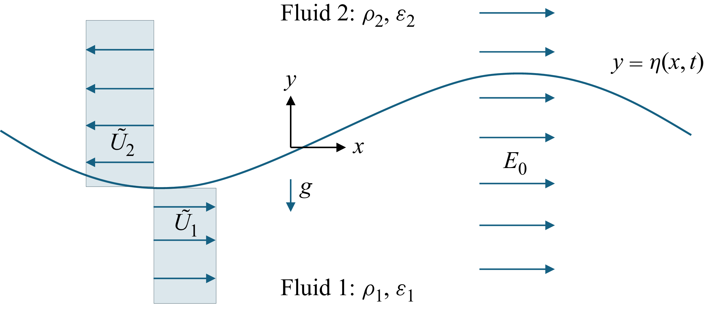
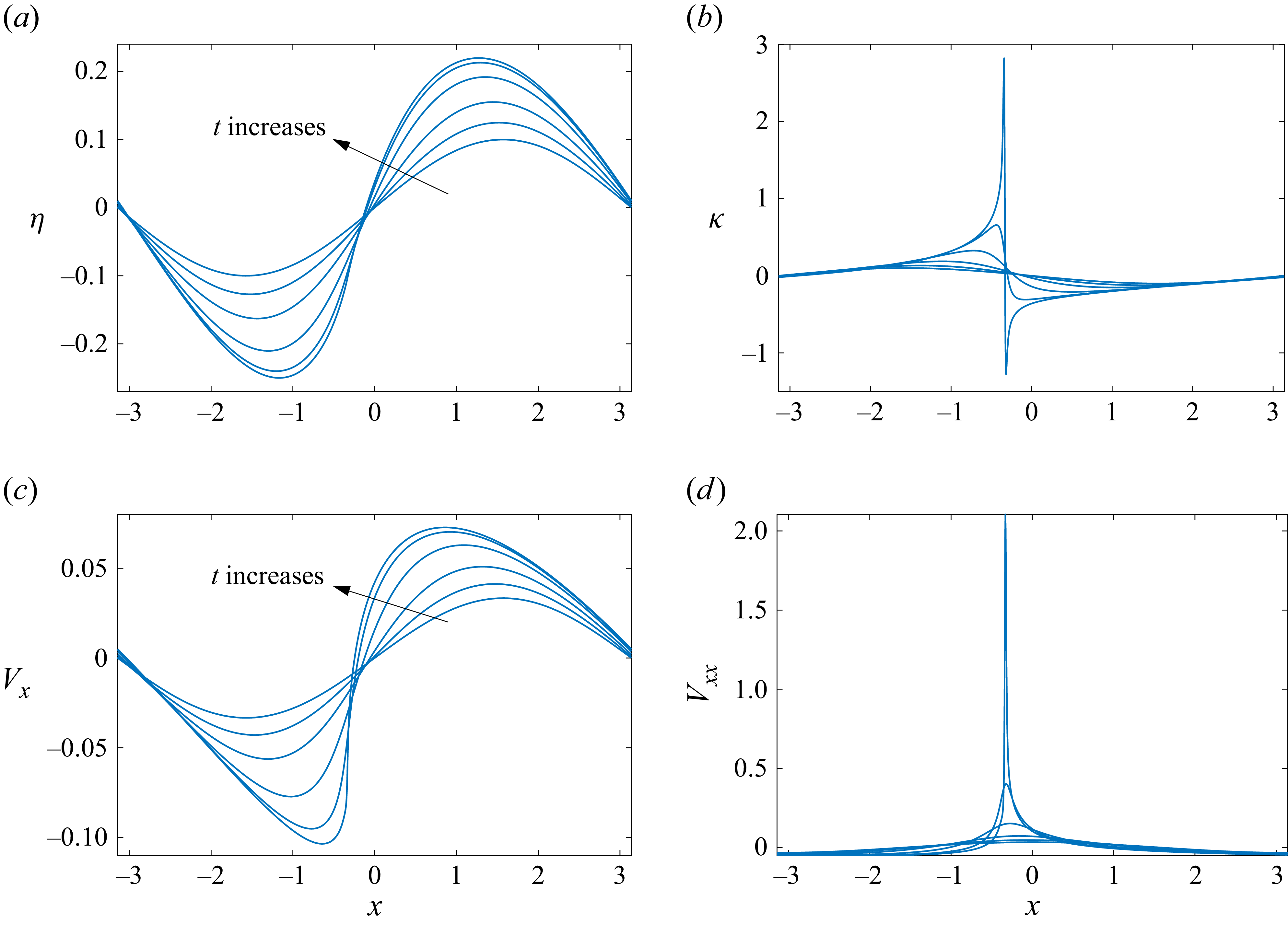
 U=1,ε=2,Eb=1
 δ=0.1
 η,κ,Vx
 Vxx
 t=0,0.8,1.6,2.4,2.8,2.92
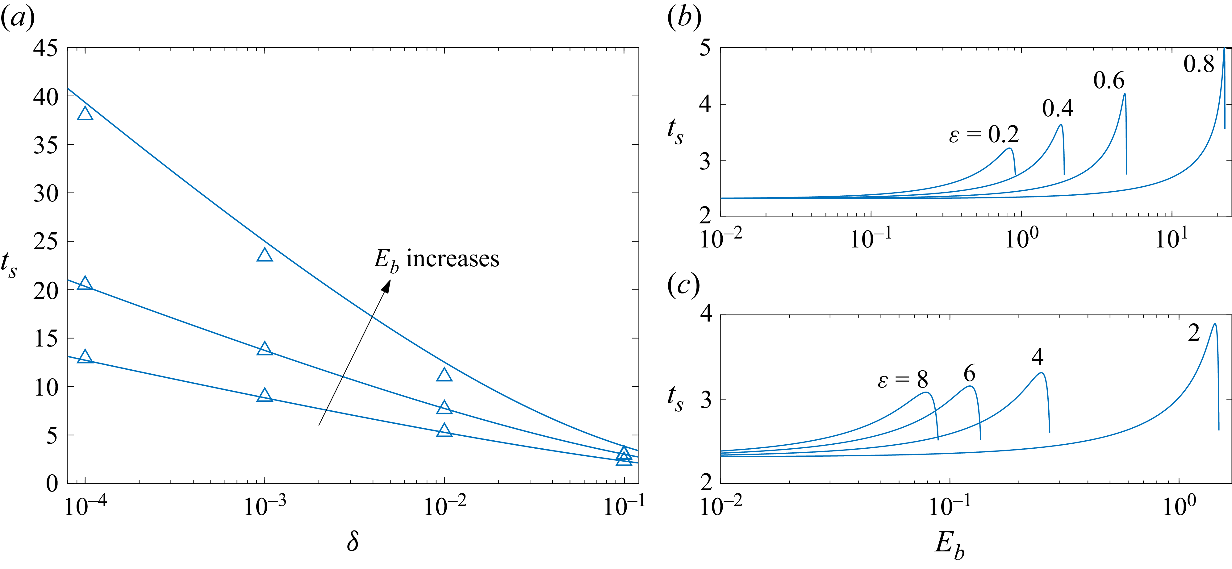
 ts
 δ
 U=1
 ε=2
 Eb=0,1,1.4
 ts
 Eb
 δ=0.1

 γ=1
 η0(ξ,0)=0.1sin(ξ)
 t=0,0.5,1,1.5,2
 2.276
 t=2.276
 t=2.35

 |γ|−1
 Eb
 cU>0
 ε<1
 ε>1
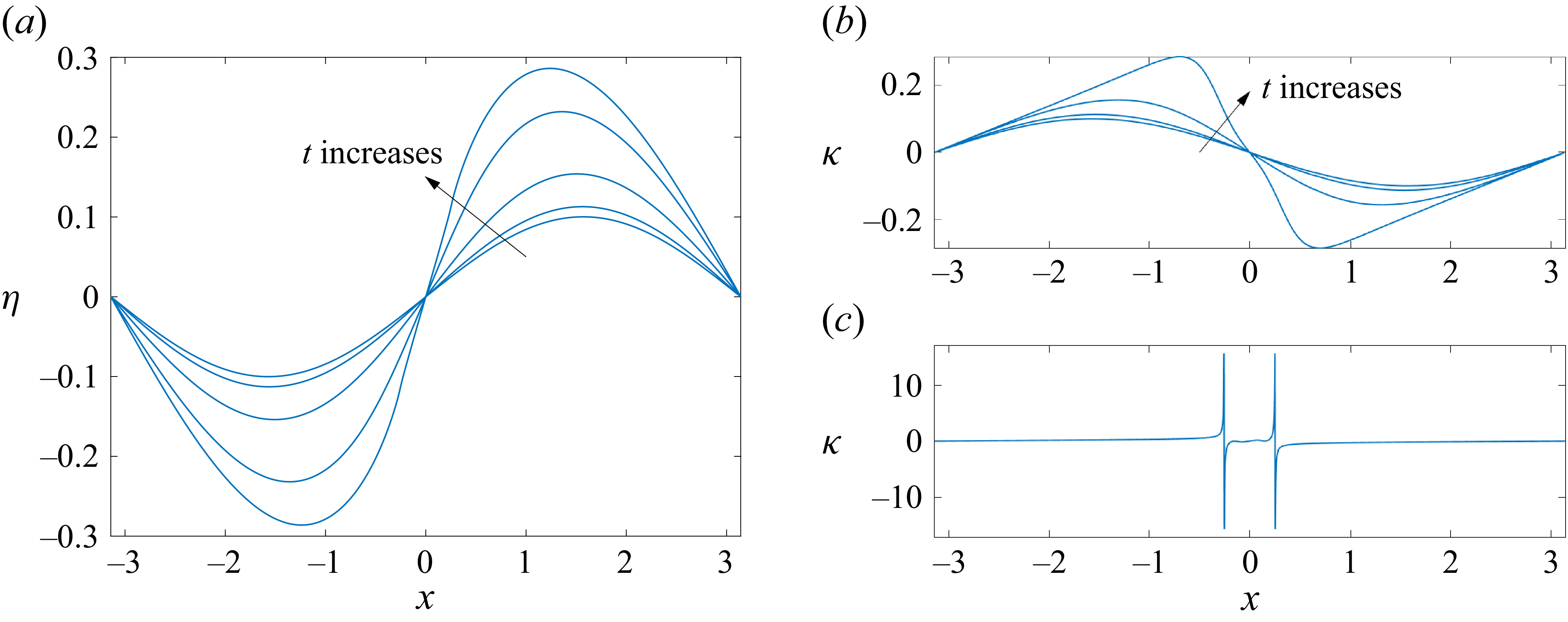
 Eb=0
 μ=0.1
 t=0,1,2,3
 3.4925
 t=0,1,2,3
 t=3.4925

 Eb=1,ε=2
 μ=0.1
 t=0,1,2,3,4
 4.5
 t=0,1,2,3,4
 t=4.4975

 Eb=1,ε=2
 μ=0.1
 Vs
 t=0,1,2,3,4
 4.5
 Vss
 t=0,1,2,3,4
 Vss
 t=4.4975
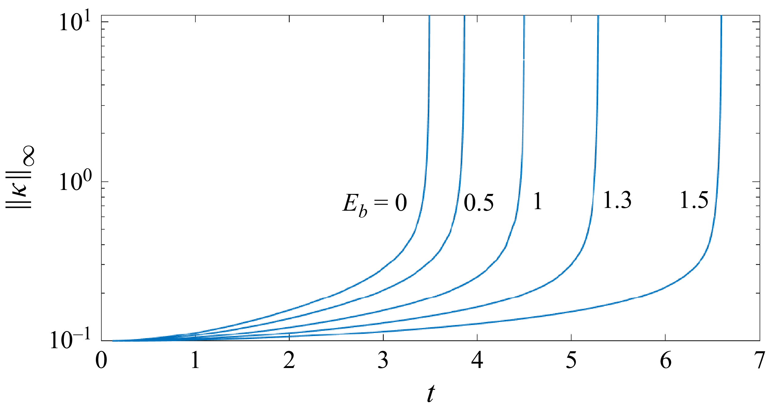
 ‖κ‖∞
 t
 Eb

 η
 θ
 Eb=5
 ε=2
 μ=0.1

 Eb=5
 ε=2
 μ=0.1
 ‖η‖∞
 t
 η
 t=13.88
 ‖κ‖∞
 t
 κ
 t=13.88
 Hr
 θ
 t=4,8,12,13.6
 13.88
 k−1.5
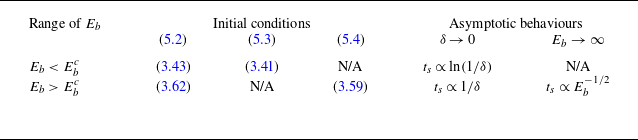
 ts
 Eb

 Eb=5
 c=0.7638
 t=0,5,10
 14.45
 θ
 t=14.45
 ‖κ‖∞
 t
 Hr

 ts
 Eb
 ε=0.5
 μ=0.1
 Ebc=3

 ts
 ε=2
 μ=0.1
 Eb=1.544
 52.46
 γ=0
 Ebc=1.5

 Eb=52.46
 ε=2
 t=0
 t=1000
 η
 κ
 t=1000
 x

 ts
 Eb
 log
 log
 ε=0.5
 μ=0.1
 Eb−1/2

 ts
 δ
 Eb=1,ε=2
 Eb=5,ε=0.5


 U=1,Eb=1
 ε=2
 η(x,0)=0.1sin(x)
 |ame−λmt|
 t∈[0,2.932]
 log
 log
 m
 1
 10
 am
 t=0,2,2.8
 2.932
 m−2.5

 Open access

