2.1. Mean wall-normal velocity at the boundary-layer edge

For a statistically steady compressible turbulent boundary layer, the mean continuity equation is (see Huang, Coleman & Bradshaw Reference Huang, Coleman and Bradshaw1995)

(2.1) \begin{align} 0 & = \dfrac {\partial (\overline {\rho }\, \widetilde {u})} {\partial x} + \dfrac {\partial (\overline {\rho } \, \widetilde {v}) }{\partial y}. \end{align}

In this study, the Reynolds decomposition of a general flow variable $\varphi$ is expressed as $\varphi = \overline {\varphi } + {\varphi '}$ , where $\overline{\varphi}$ denotes the Reynolds-averaged value and $\varphi'$ its fluctuation. The Favre (density-weighted) decomposition is written as $\varphi = \widetilde {\varphi } + \varphi ''$ , where $\widetilde{\varphi}$ is the Favre-averaged quantity and $\varphi{''}$ the corresponding fluctuation. In this notation, $\overline{\rho}$ is the Reynolds averaged density, and $\widetilde{u}$ and $\widetilde{v}$ are the Favre-averaged streamwise ( $x$ ) and wall-normal ( $y$ ) velocity components, respectively. Integrating the mean continuity (2.1) from the wall to the boundary-layer edge gives an expression for the Favre averaged mean wall-normal velocity at the boundary-layer edge as (see Appendix A for details)

(2.2) \begin{equation} \dfrac {\widetilde {v}_e}{\widetilde {u}_e} = \dfrac {\mathrm{d} \delta _1}{\mathrm{d} x} \;-\; \dfrac {(\delta _e - \delta _1)}{\widetilde {u}_e} \dfrac {\mathrm{d} \widetilde {u}_e}{\mathrm{d} x} - \dfrac {(\delta _e - \delta _1) }{\overline {\rho }_e} \dfrac {\textrm {d} \overline {\rho }_e}{\textrm {d}x}, \end{equation}

where the subscript $e$ indicates evaluation at the boundary-layer edge. For example, $\widetilde{u}_e, \widetilde{v}_e$ are the Favre-averaged streamwise and wall-normal velocity compoents at the boundary layer edge, respectively. $\delta_e$ is the boundary layer thickness, and $\overline{\rho}_e$ is the mean density at the boundary layer edge. Here, the mass displacement thickness for compressible boundary-layer flows is defined as $\delta _1 \mathrel {\stackrel {\scriptscriptstyle{\textrm{def}}}{=}} \int _0^{\delta _e} (1 - ((\overline {\rho }\, \widetilde {u})/(\overline {\rho }_e \widetilde {u}_e)))\, \textrm {d}y$ (Schlichting Reference Schlichting1979). At the boundary-layer edge, terms $\overline {\rho ' u'}$ and $\overline {\rho ' v'}$ vanish, leading to $\widetilde {u}_e = \overline {u}_e + \overline {\rho ' u'\!}_e/\overline {\rho }_e = \overline {u}_e$ and $\widetilde {v}_e = \overline {v}_e + \overline {\rho ' v'\!}_e/\overline {\rho }_e = \overline {v}_e$ . Consequently, (2.2) also applies to the Reynolds-averaged velocities.

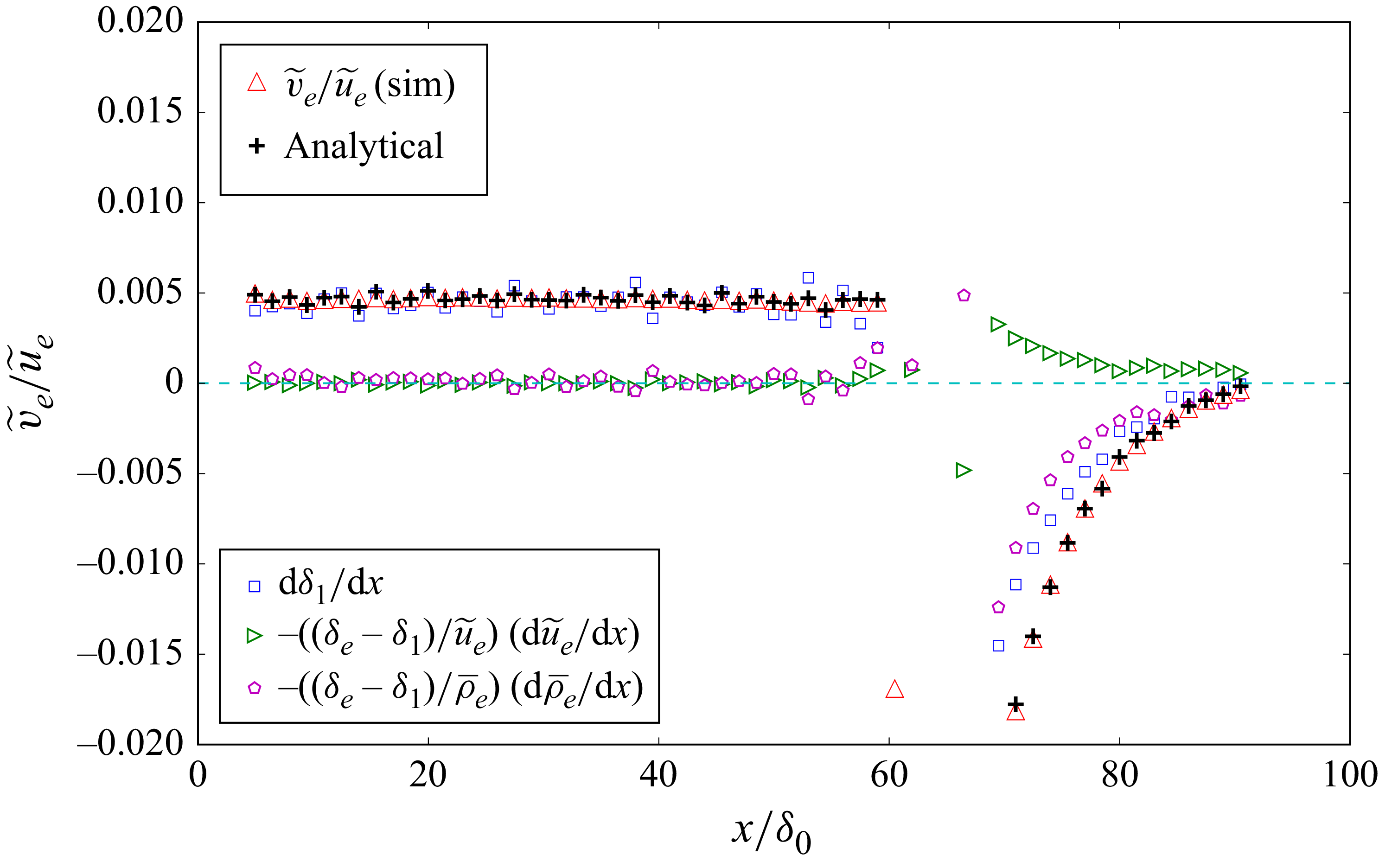
Figure 3 compares the ratio ${\widetilde {v}_e}/{\widetilde {u}_e}$ obtained from simulations with the analytical prediction of (2.2). The agreement is excellent throughout most of the domain, with noticeable discrepancies only near the impingement point. In this region, sharp streamwise variations in $\delta _e$ and $\delta _1$ (see figure 2) make accurate evaluation of the $\textrm {d}/\textrm {d}x$ terms particularly challenging in the postprocessing.

Figure 3.

Comparison of the mean wall-normal velocity at the boundary-layer edge (red triangles) and analytical (2.2) (black plus symbols). The DNS data are from Ceci et al. (Reference Ceci, Palumbo, Larsson and Pirozzoli2023).

Figure 4.

Ratio of the final two terms in (2.2), based on DNS data from Ceci et al. (Reference Ceci, Palumbo, Larsson and Pirozzoli2023).

Figure 3 also shows that $\widetilde {v}_e$ remains much smaller than $\widetilde {u}_e$ (of the order of 0.5 %) away from the impingement point, specifically for $x/\delta _0 \lt 55$ or $x/\delta _0 \gt 80$ in the simulations of Ceci et al. (Reference Ceci, Palumbo, Larsson and Pirozzoli2023). In contrast, near the impingement point, the ratio $\widetilde {v}_e/\widetilde {u}_e$ increases sharply, reaching values of approximately $-13\,\%$ at $x/\delta _0 \approx 64$ . These larger values are omitted from the figure to maintain clarity in the regions away from the impingement point.

Compared with the incompressible analytical solution of Wei et al. (Reference Wei, Li, Knopp and Vinuesa2023a ), the key distinction in compressible flow is the last term in (2.2) that accounts for streamwise variations in $\overline {\rho }_e$ . This density-gradient term is negligible far from the impingement point ( $x/\delta _0 \lesssim 55$ or $x/\delta _0 \gtrsim 80$ ), where $\widetilde {v}_e/\widetilde {u}_e$ can be accurately approximated by $\textrm {d} \delta _1/\textrm {d}x$ .

Upstream of the impingement point, the last two terms in (2.2) are negligibly small. Downstream of the impingement point, however, these terms become significant, and their profiles are closely correlated, as shown in figure 3. Their relationship can be quantified through the ratio, which, under the assumption of isentropic compressible flow, becomes

(2.3) \begin{equation} \dfrac {\dfrac {1}{\overline {\rho }_e} \dfrac {\textrm {d} \overline {\rho }_e}{\textrm {d}x}}{ \dfrac {1}{\widetilde {u}_e} \dfrac {\textrm {d} \widetilde {u}_e}{\textrm {d}x} } \; \approx - {M}^2_e, \end{equation}

where ${M}_e$ denotes the local Mach number at the boundary-layer edge (see Appendix B for details). This is checked in figure 4, where data upstream of the impingement point are omitted as both numerator and denominator are negligibly small (see figure 3). Downstream of the impingement point, we find that (2.3) applies with good accuracy.

From equations (2.3) and (2.2), the mean wall-normal velocity at the boundary-layer edge is directly related to the outer-flow Mach number. Specifically, we find that

(2.4) \begin{equation} \dfrac {\widetilde {v}_e}{\widetilde {u}_e} \approx \dfrac {\mathrm{d} \delta _1}{\mathrm{d} x} \;-\; \dfrac {(\delta _e - \delta _1)}{\widetilde {u}_e} \dfrac {\mathrm{d} \widetilde {u}_e}{\mathrm{d} x} \big ( 1 - {M}^2_e \big ) . \end{equation}

In the incompressible limit, where the density is constant and ${M}_e \to 0$ , (2.4) reduces to the mean wall-normal velocity relation for incompressible flows (Wei et al. Reference Wei, Li, Knopp and Vinuesa2023a ). This confirms that (2.4) provides a unified description that consistently extends the incompressible theory to compressible supersonic boundary layers.

2.2. Mean wall-normal velocity distribution

To derive an analytical equation for the mean wall-normal velocity, we begin by transforming the mean continuity equation into a dimensionless form. This transformation is achieved by introducing the following normalised variables:

(2.5) \begin{equation} x^* \mathrel {\stackrel {\scriptscriptstyle{\textrm{def}}}{=}} \dfrac {x}{L}, \qquad y^* \mathrel {\stackrel {\scriptscriptstyle{\textrm{def}}}{=}} \dfrac {y}{\delta _e(x)}, \qquad U^*(x^*,y^*) \mathrel {\stackrel {\scriptscriptstyle{\textrm{def}}}{=}} 1 - \dfrac {\overline {\rho } \, \widetilde {u}}{ \overline {\rho }_e \widetilde {u}_e}, \qquad V^*(x^*,y^*) \mathrel {\stackrel {\scriptscriptstyle{\textrm{def}}}{=}} \dfrac {\overline {\rho } \, \widetilde {v}}{ \overline {\rho }_e \widetilde {v}_e}, \end{equation}

where $L$ is a length scale in the $x\hbox{-}$ direction and $\delta _e$ is the boundary-layer thickness. It is important to emphasise that the use of these normalised variables does not imply the presence or absence of self-similarity in the flow. Instead, it provides a mathematical framework that facilitates the derivation and analysis of the mean wall-normal velocity.

Using the defined normalised variables, the terms in the mean continuity (2.1) can be expressed as

(2.6) \begin{align} \dfrac {\partial (\overline {\rho } \, \widetilde {u} )}{\partial x} & = \dfrac {\mathrm{d} \big(\overline {\rho }_e \widetilde {u}_e\big)}{\mathrm{d} x} -\dfrac {\mathrm{d} \big(\overline {\rho }_e \widetilde {u}_e\big)}{\mathrm{d} x} U^* + \dfrac {\overline {\rho }_e \widetilde {u}_e}{\delta _e} \dfrac {\mathrm{d} \delta _e}{\mathrm{d} x} y^* \dfrac {\partial U^*}{\partial y^*} - \dfrac {\overline {\rho }_e \widetilde {u}_e}{L} \dfrac {\partial U^*}{\partial x^*}, \end{align}

(2.7) \begin{align} \dfrac {\partial (\overline {\rho } \, \widetilde {v} )}{\partial y} & = \dfrac {\overline {\rho }_e \widetilde {v}_e}{\delta _e} \dfrac {\partial V^*}{\partial y^*}. \end{align}

Simple mathematics produces a dimensionless continuity equation in the form of

(2.8) \begin{align} \dfrac {\partial V^*}{\partial y^*} = & - \dfrac {\delta _e}{\overline {\rho }_e \widetilde {v}_e} \dfrac {\mathrm{d} \big(\overline {\rho }_e \widetilde {u}_e\big)}{\mathrm{d} x} \;+\; \left [ \dfrac {1}{\widetilde {v}_e} \dfrac {\mathrm{d} \big(\widetilde {u}_e \delta _e\big)}{\mathrm{d} x} + \dfrac {\widetilde {u}_e \delta _e}{\widetilde {v}_e} \dfrac {1}{\overline {\rho }_e} \dfrac {\textrm {d} \overline {\rho }_e}{\textrm {d}x} \right ] U^* \nonumber \\ & \;-\; \dfrac {\widetilde {u}_e}{\widetilde {v}_e} \dfrac {\mathrm{d} \delta _e}{\mathrm{d} x}\dfrac {\partial (y^* U^*)}{\partial y^*} \;+\; \dfrac {\widetilde {u}_e}{\widetilde {v}_e} \dfrac {\delta _e}{L}\dfrac {\partial U^*}{\partial x^*} . \end{align}

Integrating (2.8) with respect to $y^*$ yields an analytical equation for the mean wall-normal velocity distribution:

(2.9) \begin{align} V^* = & \underbrace {-\left [ \dfrac {\delta _e}{ \widetilde {v}_e} \dfrac {\mathrm{d} \widetilde {u}_e}{\mathrm{d} x} \right ]}_{a_{{_I}}}y^* \; \underbrace {- \left [ \dfrac {\widetilde {u}_e}{\widetilde {v}_e} \dfrac {\textrm {d} \delta _e}{\textrm {d}x} \right ]}_{a_{{_{\textit{II}}}}}y^* U^* \; + \; \underbrace {\left [ \dfrac {1}{\widetilde {v}_e} \dfrac {\textrm {d} \big(\widetilde {u}_e \delta _e\big)}{\textrm {d}x} \right ]}_{-(a_{{_{I}}}+a_{{_{\textit{II}}}})} \int _0^{y^*} U^* \textrm {d}y^* \nonumber \\ & + \; \underbrace {\left [ \dfrac {\widetilde {u}_e}{\widetilde {v}_e} \dfrac {\delta _e}{L} \right ]}_{a_{{_{\textit{III}}}}} \int _0^{y^*} \dfrac {\partial U^*}{\partial x^*}\textrm {d}y^* \; \underbrace {-\left [ \dfrac {\widetilde {u}_e }{\widetilde {v}_e} \dfrac {\delta _e}{\overline {\rho }_e} \dfrac {\textrm {d} \overline {\rho }_e}{\textrm {d}x} \right ]}_{a_{{_{_{\textit{IV}}}}}} \int _0^{y^*} (1-U^*)\, \textrm {d}y^* . \end{align}

Evaluation of (2.9) at $y^* = 1$ yields (2.2), providing the mean wall-normal velocity at the boundary-layer edge.

Figure 5.

Comparison of the simulated mean wall-normal velocity profile with the analytical prediction from (2.9). Black plus symbols represent the sum of the five components in (2.9): (a) $x/\delta _0 = 32.467$ , (b) $x/\delta _0 = 67.485$ . The DNS data are from Ceci et al. (Reference Ceci, Palumbo, Larsson and Pirozzoli2023).

As an illustration, figure 5 compares the analytical solution from (2.9) with the simulated  $V^*$ profiles at two streamwise locations: one upstream of the impingement point and one near the impingement point. In both cases, the analytical prediction shows good agreement with the simulations, accurately capturing the mean wall-normal velocity distribution across the boundary layer.

The last term in (2.9) arises from density variations and is absent in incompressible flows. As shown in figure 5, this term plays a crucial role in shaping the mean wall-normal velocity distribution in compressible boundary layers. It can be further decomposed into two contributions: a linear growth component ( $a_{{_{\textit{IV}}}} y^*$ ), and an integral component ( $a_{{_{\textit{IV}}}} \int _0^{y^*} U^*\, \textrm {d}y^*$ ). The latter approaches a constant value of $a_{{_{\textit{IV}}}} \delta _1/\delta _e$ at the boundary-layer edge. Consequently, (2.9) yields two distinct linear growth terms: the first term and the linear contribution from the density-gradient term. These linear behaviours are clearly visible in figure 5, particularly beyond the boundary-layer edge. Notably, the slope ratio of these two components, $a_{{_{\textit{IV}}}}/a_{{_{I}}}$ , matches that defined in (2.3). Since this ratio exceeds unity, the density-variation-induced contribution exhibits a steeper slope than the first term.

2.3. Analytical equation for the wall shear stress

The mean streamwise momentum equation for compressible boundary-layer flows is given by (Huang et al. Reference Huang, Coleman and Bradshaw1995)

(2.10) \begin{equation} \dfrac {\partial (\overline {\rho } \, \widetilde {u}\, \widetilde {u})}{\partial x} + \dfrac {\partial (\overline {\rho } \, \widetilde {u} \, \widetilde {v})}{\partial y} = - \dfrac {\partial \overline {p}}{\partial x} + \frac {\partial \overline {\tau }_{xy}}{\partial y} - \dfrac {\partial (\overline {\rho } \widetilde {u'' u''})}{\partial x} - \dfrac {\partial (\overline {\rho } \widetilde {u'' v''\ })}{\partial y}, \end{equation}

where $\overline{p}$ is the mean pressure, $\overline{\rho}\,\widetilde{u'' u''}$ and $\overline{\rho}\widetilde{u'' v''}$ are the Favre-averaged Reynolds normal and shear stresses, respectively, and $\overline {\tau }_{xy}$ is the mean viscous shear stress. Integrating the momentum (2.10) from the wall to the boundary-layer edge and applying the corresponding boundary conditions yields

(2.11) \begin{equation} \int _0^{\delta _e} \dfrac {\partial (\overline {\rho } \, \widetilde {u}\, \widetilde {u})}{\partial x} \textrm {d}y + \overline {\rho }_e \widetilde {u}_e \widetilde {v}_e = - \int _0^{\delta _e} \dfrac {\partial \overline {p}}{\partial x} \textrm {d}y - \tau _{w\textit{all}} - \int _0^{\delta _e} \dfrac {\partial (\overline {\rho }\, \widetilde {u'' u''})}{\partial x} \textrm {d}y .\end{equation}

Through a sequence of mathematical manipulations (see Appendix C), the momentum integral equation is derived:

(2.12) \begin{align} \tau _{w\textit{all}} \;= & \; \underbrace {\overline {\rho }_e \widetilde {u}_e \delta _1 \dfrac {\textrm {d} \widetilde {u}_e}{\textrm {d}x}}_{\mathrm{I}} \;+\ \underbrace {\overline {\rho }_e \dfrac {\textrm {d}\big( \widetilde {u\,}^2_e\delta _2 \big)}{\textrm {d}x}}_{\mathrm{II}} \; \underbrace {- \dfrac {\textrm {d}}{\textrm {d}x} \left ( \int _0^{\delta _e} (\overline {\rho }\, \widetilde {u'' u''})\, \textrm {d}y\right )}_{\mathrm{III}} \nonumber \\[10pt] & \underbrace {- \int _0^{\delta _e} \left ( \dfrac {\partial \overline {p}}{\partial x} + \overline {\rho }_e \widetilde {u}_e \dfrac {\textrm {d} \widetilde {u}_e}{\textrm {d}x} \right ) \textrm {d} y }_{\mathrm{IV}} \; +\; \underbrace { \widetilde {u}^2_e \delta _2 \dfrac {\textrm {d} \overline {\rho }_e}{\textrm {d}x}}_{\mathrm{V}} , \end{align}

where $\delta _2 = \int _0^{\delta _e} (\overline {\rho } \widetilde {u})/( \overline {\rho }_e \widetilde {u}_e) ( 1- \widetilde {u}/\widetilde {u}_e)\, \textrm {d}y$ is the momentum thickness defined for compressible flows (Schlichting Reference Schlichting1979).

For incompressible flow, where the density is constant, the first two terms on the right-hand side of (2.12) reduce to the classical Kármán–Pohlhausen momentum integral equation (von Kármán Reference von Kármán1921; Pohlhausen Reference Pohlhausen1921; Gruschwitz Reference Gruschwitz1931).

In studies of incompressible boundary layers with pressure gradients, Wei, Li & Wang (Reference Wei, Li and Wang2024) demonstrated that the commonly assumed relation $\partial \overline {p}/\partial x = - \rho \overline {u}_e \, \textrm {d}\overline {u}_e/\textrm {d}x$ fails under strong pressure gradients, as $\partial \overline {p}/\partial x$ exhibits pronounced wall-normal variation. To account for this effect, Wei et al. (Reference Wei, Li, Knopp and Vinuesa2023a ) introduced an additional contribution (term IV) into the momentum integral formulation, thereby extending the classical Kármán–Pohlhausen formulation.

In compressible turbulent boundary layers, the streamwise pressure gradient $\partial \overline {p}/\partial x$ also exhibits pronounced wall-normal variation when the flow is subjected to strong pressure gradients, as shown in figure 6. The figure presents profiles of $\partial \overline {p}/\partial x$ at four streamwise locations. Away from the impingement region (e.g. $x/\delta _0 = 40$ and $x/\delta _0 = 80$ ), the pressure gradient remains nearly uniform in the wall-normal direction. In contrast, closer to the impingement point (e.g. $x/\delta _0 = 60$ and $x/\delta _0=64$ ), $\partial \overline {p}/\partial x$ shows significant wall-normal variation. The inclusion of term IV in (2.12) explicitly accounts for these wall-normal variations of $\partial \overline {p}/\partial x$ , thereby improving the prediction of wall shear stress near the impingement point.

Figure 6.

Wall-normal distributions of the streamwise pressure gradient $\partial \overline {p}/\partial x$ at four $x$ -locations.

For compressible turbulent boundary layers, the general form of the momentum integral (2.12) introduces an additional term V, which arises from density variations, hence not present in the incompressible case (Wei et al. Reference Wei, Li and Wang2024). Note that the ratio of term V to term I in the momentum integral (2.12) is directly connected to the ratio given in (2.3), namely

(2.13) \begin{equation} \dfrac { \widetilde {u\,}^2_e \delta _2 \dfrac {\textrm {d} \overline {\rho }_e}{\textrm {d}x} }{ \overline {\rho }_e \widetilde {u}_e \delta _1 \dfrac {\textrm {d} \widetilde {u}_e}{\textrm {d}x} } \; = \; \dfrac {1}{H_{12}} \dfrac {\dfrac {1}{\overline {\rho }_e} \dfrac {\textrm {d} \overline {\rho }_e}{\textrm {d}x}}{ \dfrac {1}{\widetilde {u}_e} \dfrac {\textrm {d} \widetilde {u}_e}{\textrm {d}x} } , \end{equation}

where $H_{12} = \delta_1/\delta_2$ is the shape factor. Figure 7 evaluates the momentum integral (2.12) using DNS data from Ceci et al. (Reference Ceci, Palumbo, Larsson and Pirozzoli2023). The analytical predictions, shown as black plus symbols, demonstrate excellent agreement with the DNS results. The scatter observed in the comparison arises primarily from numerical errors introduced during the numerical evaluation of the streamwise derivatives. Upstream of the impingement point ( $x/\delta _0 \lesssim 55$ ), the second term on the right-hand side of (2.12) dominates the wall shear stress, while all other contributions remain negligible. In contrast, downstream of the impingement point, term I (associated with the pressure gradient) and term IV (arising from pressure-gradient variations in the wall-normal direction) become significant. Term V (arising from density gradient) in (2.12) plays a crucial role downstream of the impingement point, as illustrated in figure 7. In contrast, DNS data from Ceci et al. (Reference Ceci, Palumbo, Larsson and Pirozzoli2023) indicate that the contribution from the turbulent normal stress, $\overline {\rho }\,\widetilde {u'' u''}$ (term III), remains small throughout the domain, including the region around the impingement point.

Figure 7.

Comparison of the mean momentum integral (2.12) with DNS data from Ceci et al. (Reference Ceci, Palumbo, Larsson and Pirozzoli2023).

Schlichting (Reference Schlichting1979) presented a momentum integral equation for compressible laminar boundary-layer flows, assuming that pressure remains constant across the boundary layer. As a result, his formulation is limited to laminar flows subjected to zero or weak pressure gradients. In contrast, (2.12) is more general and applicable to both laminar and turbulent compressible boundary layers under arbitrary pressure-gradient conditions.

By substituting the analytical expression for $\widetilde {v}_e$ from (2.2) into the integral momentum (2.12), the latter can be recast into an alternative form, as detailed in the Appendix C:

(2.14) \begin{align} \dfrac {\overline {\rho }_e \, \widetilde {u}_e \, \widetilde {v}_e}{\tau _{w\textit{all}}} = & \; H_{_{12}} \;+\; \dfrac { \overline {\rho }_e \, \widetilde {u\,}^2_e \,\delta _1 }{\tau _{w\textit{all}}}\, \dfrac {1}{H_{_{12}}} \dfrac {\textrm {d} H_{_{12}}}{\textrm {d}x} \; + \; \dfrac {H_{_{12}}}{\tau _{w\textit{all}}} \dfrac {\textrm {d}}{\textrm {d}x} \left ( \int _0^{\delta _e} (\overline {\rho }\, \widetilde {u'' u''\ }) \textrm {d}y\right ) \nonumber \\[10pt] & \; + \; \dfrac {H_{_{12}}}{\tau _{w\textit{all}}} \int _0^{\delta _e} \left ( \dfrac {\partial \overline {p}}{\partial x} + \overline {\rho }_e \widetilde {u}_e \dfrac {\textrm {d} \widetilde {u}_e}{\textrm {d}x} \right ) \textrm {d} y \; - \ \left ( 1 + \dfrac {\delta _e}{\delta _1} + H_{_{12}} \right ) \dfrac { \overline {\rho }_e \, \widetilde {u}_e \, \delta _1}{\tau _{w\textit{all}}} \, \dfrac {\textrm {d} \widetilde {u}_e}{\textrm {d}x} \; - \; \dfrac { \widetilde {u\,}^2_e \delta _e }{\tau _{w\textit{all}}}\, \dfrac {\textrm {d}\overline {\rho }_e}{\textrm {d}x}. \end{align}

Figure 8.

Comparison of the analytical expression for wall shear stress, (2.14), with DNS data from Ceci et al. (Reference Ceci, Palumbo, Larsson and Pirozzoli2023).

Figure 8 presents a comparison between the analytical (2.14) and the DNS data from Ceci et al. (Reference Ceci, Palumbo, Larsson and Pirozzoli2023). Overall, the analytical predictions show good agreement with the DNS results, demonstrating the accuracy of the derived equation.

For compressible boundary-layer flows subjected to weak pressure gradients, only the term $H_{_{12}}$ on the right side of (2.14) remains significant, while the contributions of the other terms become negligible. Consequently, for such flows, (2.14) simplifies to $(\overline {\rho }_e \, \widetilde {u}_e \, \widetilde {v}_e)/\tau _{w\textit{all}} \approx \; H_{_{12}}$ , as illustrated in figure 8 for $x/\delta _0 \lt 55$ . Note that the counterpart for incompressible zero-pressure-gradient turbulent boundary layer is $({\overline {u}_e \, \overline {v}_e})/{u^2_\tau } \approx \; H_{_{12}}$ (see Wei & Klewicki Reference Wei and Klewicki2016, Reference Wei and Klewicki2023).

By straightforward manipulation, (2.14) can be recast into a form suitable for evaluating the skin-friction coefficient, $C_f = \tau _{w\textit{all}}/(0.5 \, \overline {\rho }_e \, \widetilde {u\,}^2_e)$ , as

(2.15) \begin{align} C_f = & \dfrac {2}{H_{12}} \left \{\, \dfrac {\widetilde {v}_e}{\widetilde {u}_e} - \dfrac {\delta _1}{H_{12}}\dfrac {\textrm {d}H_{12} }{\textrm {d}x} + \left ( 1 + \dfrac {\delta _e}{\delta _1} + H_{_{12}} \right ) \dfrac {\delta _1}{\widetilde {u}_e}\dfrac {\textrm {d}\widetilde {u}_e }{\textrm {d}x} \right. \nonumber \\[8pt] & - \left. \dfrac {H_{12}}{\overline {\rho }_e\, \widetilde {u\,}^2_e}\left ( \dfrac {\textrm {d}}{\textrm {d}x} \int _0^{\delta _e} \big(\overline {\rho }\, \widetilde {u'' u''} \big) \textrm {d}y + \int _0^{\delta _e} \left ( \dfrac {\partial \overline {p}}{\partial x} + \overline {\rho }_e \widetilde {u}_e \dfrac {\textrm {d} \widetilde {u}_e}{\textrm {d}x} \right ) \textrm {d} y\right ) \, + \dfrac {\delta _e}{\overline {\rho }_e} \dfrac {\textrm {d} \overline {\rho }_e}{\textrm {d}x} \right \}\!.\end{align}

This formulation expresses the skin-friction coefficient as a function of key boundary-layer parameters, including $\widetilde {u}_e$ , $\widetilde {v}_e$ , $H_{_{12}}$ and others, which evolve along the streamwise direction. Figure 9 compares the simulated friction coefficient $C_f$ with the analytical prediction from (2.15) and its individual components, showing good overall agreement.

Under weak pressure-gradient conditions, $C_f$ is governed primarily by the first term on the right-hand side of (2.15). Downstream of the impingement point, where the DNS results indicate flow separation, $C_f$ becomes more strongly influenced by the terms involving $\widetilde {v}_e$ (first term on the right-hand side), $\textrm {d}H_{_{12}}/\textrm {d}x$ (second term), the pressure gradient (third term) and the density gradient (last term). During and following boundary-layer separation, $\widetilde {v}_e$ (or the first term) becomes negative–indicating entrainment of free-stream fluid into the boundary layer. At the same time, $H_{_{12}}$ decreases rapidly in the streamwise direction, leading to a positive contribution from the second term. In compressible boundary-layer flows, density variations (last term) also play a significant role in determining the skin-friction coefficient, particularly in regions of strong pressure gradients.

Figure 9.

Comparison of the analytical expression for the friction coefficient, (2.15), with DNS data from Ceci et al. (Reference Ceci, Palumbo, Larsson and Pirozzoli2023).

In free-shear turbulent flows, such as wakes and jets, the mean transverse velocity is much smaller than the mean axial velocity. Nevertheless, studies have demonstrated that it plays a key role in scaling turbulence quantities, including the turbulent shear stress (Wei & Livescu Reference Wei and Livescu2021; Wei, Livescu & Liu Reference Wei, Livescu and Liu2022). A similar situation arises in turbulent boundary-layer flows, where the mean wall-normal velocity is also much smaller than the streamwise velocity and is virtually impossible to measure directly in physical experiments. Consequently, the mean wall-normal velocity has often been overlooked in previous studies of boundary layers. Despite its small magnitude, the mean wall-normal velocity at the boundary-layer edge, $\widetilde {v}_e$ , is closely related to the skin-friction coefficient, as shown in (2.15).