
 m=3
 pB=1
 pR∈[0,1]
 m=3
 pB
 pR















1. Introduction
1.1. Overview of our learning model
For any positive integer m with
 $m \geqslant 2$
, let
 $\mathbb{T}_{m}$
indicate the infinite rooted tree, with root
 $\phi$
, in which each vertex has precisely m children. Let
 $V(\mathbb{T}_{m})$
denote the set of all vertices of
 $\mathbb{T}_{m}$
, and imagine an agent occupying each vertex of
 $V(\mathbb{T}_{m})$
. We consider a learning model in which each agent, at each time step (where time is indexed by the set
 $\mathbb{N}_{0}$
of non-negative integers), has to adopt one of two possible technologies that we henceforth refer to as colours or states and denote by the letters B and R. The state of the agent at a vertex
 $v \in V(\mathbb{T}_{m})$
at time step t, for each
 $t \in \mathbb{N}_{0}$
, is denoted by
 $C_{t}(v)$
. Conditioned on the states of the agents at all the vertices of
 $V(\mathbb{T}_{m})$
at time step t, the (random) state
 $C_{t+1}(v)$
to which the agent at v updates itself at time step
 $t+1$
has a probability distribution that is a function of
 $C_{t}(v_{1}), C_{t}(v_{2}), \ldots, C_{t}(v_{m})$
, where
 $v_{1}, v_{2}, \ldots, v_{m}$
are the children of v.
Such a model can be viewed from a number of different perspectives, such as
-
(i) as a discrete-time interacting system of particles on
 $\mathbb{T}_{m}$
with infinitely many changes allowed to happen at each time step,
-
(ii) as a model for social learning, for understanding the diffusion of technologies throughout an infinite population of agents, and
-
(iii) as a probabilistic finite state tree automaton on
$\mathbb{T}_{m}$
.


We delve deeper into each of the above motivating reasons for the study of such models in Subsection 1.4.
Each model studied in this paper admits a crucial component known as a policy function: it governs how the agent at v, for each
 $v \in V(\mathbb{T}_{m})$
, learns from the states
 $C_{t}(v_{i})$
,
 $i \in \{1,2,\ldots,m\}$
, of the agents situated at the children
 $v_{1}, v_{2}, \ldots, v_{m}$
of v at time step t, and subsequently updates its own state to
 $C_{t+1}(v)$
at time step
 $t+1$
. When such a model is viewed as a probabilistic tree automaton (PTA), as explained in Subsection 1.4, the policy function is referred to as the stochastic update rule associated with that PTA. We are concerned with studying the absolute majority policy function, which we describe in detail in Subsection 1.2.
1.2. Absolute majority policy
In this model, the agent occupying vertex v, for each
 $v \in V(\mathbb{T}_{m})$
, is endowed with two random variables,
 $X_{t}(v)$
and
 $Y_{t}(v)$
, for each time step
 $t \in \mathbb{N}_{0}$
. For each
 $v \in V(\mathbb{T}_{m})$
and each
 $t \in \mathbb{N}_{0}$
, the random variable
 $X_{t}(v)$
captures the outcome of the (random) experiment performed by the agent located at v, during the time step or epoch t, using the technology
 $C_{t}(v)$
that this agent is currently equipped with. This experiment has two possible outcomes—success and failure—so
 $X_{t}(v)$
is a Bernoulli random variable that acts as an indicator for the event of success. We let
 $X_{t}(v)$
follow Bernoulli
 $(\, p_{B})$
conditioned on
 $C_{t}(v)=B$
, and we let
 $X_{t}(v)$
follow Bernoulli
 $(\, p_{R})$
conditioned on
 $C_{t}(v)=R$
, where
 $p_{B}, p_{R} \in [0, 1]$
are preassigned parameters in our model. The random variable
 $Y_{t}(v)$
follows Bernoulli
 $\left(\frac{1}{2}\right)$
for each
 $v \in V(\mathbb{T}_{m})$
and each
 $t \in \mathbb{N}_{0}$
. It is assumed that the entire collection
 $\left\{X_{t}(v)\,:\, v \in V(\mathbb{T}_{m})\right\}\cup\left\{Y_{t}(v)\,:\, v \in V(\mathbb{T}_{m})\right\}$
of random variables is independent for each time step
 $t \in \mathbb{N}_{0}$
, and the collection
 $\left\{Y_{t}(v)\,:\, v \in V(\mathbb{T}_{m})\right\}$
is independent of
 $\left\{C_{s}(u)\,:\, u \in V(\mathbb{T}_{m}), s \in \{0,1,\ldots,t\}\right\}$
for each
 $t \in \mathbb{N}_{0}$
.
Conditioned on
 $\left\{C_{t}(u)\,:\, u \in V(\mathbb{T}_{m})\right\}$
, the agent at v updates its state to
 $C_{t+1}(v)$
according to the following rule, where
 $v_{1}, v_{2}, \ldots, v_{m}$
denote the children of v:
 \begin{equation} C_{t+1}(v) = \begin{cases} B & \text{if } \sum_{i=1}^{m}X_{t}(v_{i})\mathbf{1}_{C_{t}(v_{i})=B} > \sum_{i=1}^{m}X_{t}(v_{i})\mathbf{1}_{C_{t}(v_{i})=R}, \\[3pt] B & \text{if } \sum_{i=1}^{m}X_{t}(v_{i})\mathbf{1}_{C_{t}(v_{i})=B} = \sum_{i=1}^{m}X_{t}(v_{i})\mathbf{1}_{C_{t}(v_{i})=R} \text{ and } Y_{t}(v)=1, \\[3pt] R & \text{otherwise.} \end{cases}\end{equation}
In words, this can be described as follows: the agent at the vertex v counts the number
 $\sum_{i=1}^{m}X_{t}(v_{i})\mathbf{1}_{C_{t}(v_{i})=B}$
of successful experiments performed, during epoch t, by all those agents that occupy the children of v and that are in state B at time step t, and likewise, it also counts the number
 $\sum_{i=1}^{m}X_{t}(v_{i})\mathbf{1}_{C_{t}(v_{i})=R}$
of successful experiments performed, during epoch t, by all those agents that occupy the children of v and that are in state R at time step t. If the former count strictly exceeds the latter then the agent at v updates its state to B at time step
 $t+1$
, while if the latter strictly exceeds the former then the agent at v updates its state to R at time step
 $t+1$
. If the two counts are equal then the agent at v tosses a fair coin in order to break the tie. If the coin lands as a head, indicated by
 $Y_{t}(v)=1$
, then the agent at v updates its state to B at time step
 $t+1$
, and if the coin lands as a tail, it updates its state to R at time step
 $t+1$
.
We begin the process at time step
 $t=0$
with an independent and identically distributed (i.i.d.) assignment of states to the vertices of
 $\mathbb{T}_{m}$
, i.e. the collection
 $\left\{C_{0}(v)\,:\, v \in V(\mathbb{T}_{m})\right\}$
is i.i.d. with
 \begin{equation}C_{0}(v)=B \text{ with probability } \pi_{0} \text{ and } C_{0}(v)=R \text{ with probability } 1-\pi_{0}\end{equation}
for each
 $v \in V(\mathbb{T}_{m})$
. Letting
 $\nu_{t}$
denote the joint law of
 $\left\{C_{t}(v)\,:\, v \in V(\mathbb{T}_{m})\right\}$
for each
 $t \in \mathbb{N}_{0}$
, we are concerned in this paper with answering the following question: does
 $\left\{\nu_{t}\right\}_{t \in \mathbb{N}_{0}}$
converge as
 $t \rightarrow \infty$
, and if it does, what is its distributional limit? We investigate this question for all values of
 $(\, p_{B},p_{R}) \in [0, 1]^{2}$
when
 $m=2$
, whereas when
 $m \geqslant 3$
, we consider two regimes of values of the parameter pair
 $(\, p_{B},p_{R})$
. The first of these regimes is where
 $p_{B}=p_{R}=p$
for some
 $p \in [0, 1]$
, i.e. an agent, located at any vertex of
 $\mathbb{T}_{m}$
, stands the same chance of achieving a successful outcome in the experiment performed during epoch t irrespective of whether its state at time step t is B or R. We present a full description of what happens in such a scenario as the common value p of the two parameters is allowed to vary over [0, 1]. The complement of this regime is where
 $p_{B} \neq p_{R}$
, but when
 $m \geqslant 3$
, the analysis for
 $p_{B} \neq p_{R}$
, without additional assumptions, quickly becomes intractable, and it becomes difficult to conclude anything about the distributional limit(s) of
 $\left\{\nu_{t}\right\}_{t \in \mathbb{N}_{0}}$
(depending on the initial distribution
 $\nu_{0}$
given by (2), and on the values of
 $p_{B}$
and
 $p_{R}$
). We, therefore, focus on the special case of
 $p_{B}=1$
and
 $p_{R} \in [0,1)$
, and we demonstrate, via the relatively less unwieldy examples of
 $m=2$
and
 $m=3$
, that the conclusion is rather non-intuitive and further investigations are warranted. This special case can be considered ‘extremal’ in the sense that a vertex that is in state B is sure to achieve success when it performs its experiment (using technology B), since
 $p_{B}=1$
, whereas the experiment performed (with technology R) by a vertex in state R has a positive probability of resulting in a failure. Intuition seems to suggest that in such a scenario, eventually, every vertex of
 $\mathbb{T}_{m}$
would opt for the (evidently superior) technology B, but it turns out (see Section 5) that this is not necessarily the case, and the distributional limit depends heavily on the value of
 $p_{R}$
.
1.3. Main results
We begin with a result that is applicable to all values of the parameter pair
 $(\, p_{B},p_{R})$
.
Theorem 1. Recall that
 $\nu_{t}$
indicates the joint law of
 $\left\{C_{t}(v)\,:\, v \in V(\mathbb{T}_{m})\right\}$
for each
 $t \in \mathbb{N}_{0}$
, and recall that we begin from an i.i.d. assignment of states (from
 $\{B,R\}$
) to the vertices of
 $\mathbb{T}_{m}$
, as described in (2). The following are true.
-
(i) For each
$t \in \mathbb{N}$
, the random variables
$C_{t}(v)$
, for
$v \in V(\mathbb{T}_{m})$
, are i.i.d. with (3)for each
\begin{equation}C_{t}(v)=B \,{ with\ probability }\ \pi_{t} \text{ and } C_{t}(v)=R \ { with\ probability }\ 1-\pi_{t}\end{equation}
$v \in V(\mathbb{T}_{m})$
.
-
(ii) The sequence
$\{\nu_{t}\}_{t \in \mathbb{N}_{0}}$
converges if and only if the sequence
$\{\pi_{t}\}_{t \in \mathbb{N}_{0}}$
converges, as
$t \rightarrow \infty$
, and in that case, if
$\pi = \lim_{t \rightarrow \infty}\pi_{t}$
then
$\{\nu_{t}\}_{t \in \mathbb{N}_{0}}$
converges to
$\nu$
, where
$\nu$
is the joint law of the collection
$\left\{C_{\infty}(v)\,:\, v \in V(\mathbb{T}_{m})\right\}$
of i.i.d. random variables
$C_{\infty}(v)$
, where (4)for each
\begin{equation}C_{\infty}(v) = B \ { with\ probability }\ \pi \ { and }\ C_{\infty}(v) = R \ { with\ probability }\ 1-\pi\end{equation}
$v \in V(\mathbb{T}_{m})$
.
-
(iii) The limit
$\pi = \lim_{t \rightarrow \infty}\pi_{t}$
, when it exists, is a fixed point of the function
$g_{m} \, : \, [0, 1] \rightarrow [0, 1]$
defined as (5)in which
\begin{equation}g_{m}(x) = \sum_{k=0}^{m}f_{m}(k) \binom{m }{ k} x^{k}(1-x)^{m-k},\end{equation}
(6)where the random variable
\begin{equation}f_{m}(k) = \operatorname{\mathbb{P}}\left[A_{k} > B_{m-k}\right] + \frac{1}{2}\operatorname{\mathbb{P}}\left[A_{k} = B_{m-k}\right],\end{equation}
$A_{k}$
follows Binomial
$(k,p_{B})$
, the random variable
$B_{m-k}$
follows Binomial
$(m-k,p_{R})$
, and
$A_{k}$
and
$B_{m-k}$
are independent of each other.


From the last assertion made in the statement of Theorem 1, it becomes apparent that we need to answer the following questions.
-
(i) Does the function
$g_{m}$
have a unique fixed point in [0, 1]? -
(ii) If
$g_{m}$
has multiple fixed points in [0, 1], which of these are attractive and which are repulsive?


Let us now make the following simple observation.
Remark 1. When
 $g_{m}$
has a unique fixed point, say
 $\pi$
, in [0, 1], it must be attractive, i.e. no matter what value
 $\pi_{0} \in [0, 1]$
we choose in (2), the sequence of laws
 $\{\nu_{t}\}_{t \in \mathbb{N}_{0}}$
converges, as
 $t \rightarrow \infty$
, to
 $\nu$
defined by (4).
Proof. Let us consider any subsequence
 $\left\{\pi_{t_{k}}\right\}_{k \in \mathbb{N}}$
of the sequence
 $\{\pi_{t}\}_{t \in \mathbb{N}_{0}}$
(defined in (3)). Since this subsequence is bounded, it has a further subsequence, say
 $\left\{\pi_{t_{k_{\ell}}}\right\}_{\ell \in \mathbb{N}}$
, that converges as
 $\ell \rightarrow \infty$
. From 1 of Theorem 1, we know that
 $\lim_{\ell \rightarrow \infty}\pi_{t_{k_{\ell}}}$
has to be a fixed point of
 $g_{m}$
, and as
 $g_{m}$
has a unique fixed point,
 $\pi$
, in [0, 1], we must have
 $\lim_{\ell \rightarrow \infty}\pi_{t_{k_{\ell}}}=\pi$
. This allows us to conclude that the entire sequence
 $\{\pi_{t}\}_{t \in \mathbb{N}_{0}}$
converges to
 $\pi$
as
 $t\rightarrow \infty$
, and the rest of the conclusion in Remark 1 follows from 1 of Theorem 1.
Before moving on to higher values of m, we state the following result concerning
 $m=2$
and all possible values of
 $p_{B}$
and
 $p_{R}$
.
Theorem 2. The function
 $g_{2}$
is strictly convex for
 $p_{R} > p_{B}$
, strictly concave for
 $p_{R} < p_{B}$
, and linear for
 $p_{B}=p_{R}$
. In each of these cases, except when
 $p_{B}=p_{R}=1$
, the function
 $g_{2}$
has a unique fixed point in (0, 1). When
 $p_{B}=p_{R}=1$
, the entire interval [0, 1] constitutes the set of fixed points of
 $g_{2}$
.
From Remark 1, it is evident that for
 $m=2$
and when
 $(\, p_{B},p_{R}) \neq (1,1)$
, the sequence
 $\{\nu_{t}\}_{t \in \mathbb{N}_{0}}$
converges to
 $\nu$
, as
 $t \rightarrow \infty$
, where
 $\nu$
is as defined by (4), with
 $\pi$
being the unique fixed point of
 $g_{2}$
. For
 $m=2$
and
 $p_{B}=p_{R}=1$
, for each
 $\pi_{0} \in [0, 1]$
(where
 $\pi_{0}$
is as defined in (2)), the law
 $\nu_{t}$
is the same as
 $\nu_{0}$
for every
 $t \in \mathbb{N}$
, so the limit equals
 $\nu_{0}$
itself.
We now come to the two specific regimes of values of the parameter pair
 $(\, p_{B},p_{R})$
that, as mentioned towards the end of Subsection 1.2, are considered in this paper. When
 $p_{B}=p_{R}=p$
for some
 $p \in [0, 1]$
, the learning model with the absolute majority policy described in Subsection 1.2 admits the following phase transition phenomenon.
Theorem 3. Recall the function
 $g_{m}$
defined in (5), and consider
 $p_{B}=p_{R}=p$
in the definition of the function
 $f_{m}$
in (6). For each
 $m \in \mathbb{N}$
with
 $m \geqslant 2$
, there exists
 $p(m) \in (0,1)$
such that
-
(i) for all
$p \leqslant p(m)$
, the function
$g_{m}$
has a unique fixed point in [0, 1], which is
$1/2$
; -
(ii) for all
$p > p(m)$
, the function
$g_{m}$
has precisely three fixed points in [0, 1], of the form
$\alpha$
,
$1/2$
, and
$1-\alpha$
, where
$\alpha=\alpha(p,m) < 1/2$
is some function of p and m.


Recall
 $\pi_{t}$
from (3), for each
 $t \in \mathbb{N}$
. For every choice of the initial distribution (i.e. for every choice of
 $\pi_{0}$
, as defined in (2)), the sequence
 $\{\pi_{t}\}_{t \in \mathbb{N}_{0}}$
converges, as
 $t \rightarrow \infty$
, to
 $\pi$
(as defined in the statement of Theorem 1). Here,
 $\pi=1/2$
for each
 $\pi_{0} \in [0, 1]$
when
 $p \leqslant p(m)$
, whereas when
 $p > p(m)$
, we have (i)
 $\pi=\alpha$
when
 $\pi_{0} \in [0,1/2)$
, (ii)
 $\pi=1/2$
when
 $\pi_{0}=1/2$
, and (iii)
 $\pi=1-\alpha$
when
 $\pi_{0} \in (1/2,1]$
.
Remark 2. Note that in the regime where
 $p \leqslant p(m)$
, since
 $g_{m}$
has a unique fixed point in [0, 1], and this equals
 $1/2$
, by Remark 1 we already know that
 $\pi=1/2$
for each
 $\pi_{0} \in [0, 1]$
. Therefore, in the last assertion made in the statement of Theorem 3, we need focus only on the regime where
 $p > p_{m}$
.
In particular, we show, via analytical methods in Subsection 4.1, that for
 $m=3$
, the threshold
 $p(m) \approx 0.557507$
, whereas for
 $m=4$
, the threshold
 $p(m) \approx 0.42842$
.
When
 $p_{B}=1$
and
 $p_{R} \in [0,1)$
, our learning model is devoid of any phase transition for
 $m=2$
(which follows as a special case of Theorem 2), whereas a striking and rather non-intuitive phenomenon of phase transition is observed when
 $m=3$
, as stated below.
Theorem 4. When
 $m=3$
,
 $p_{B}=1$
, and
 $p_{R} \in [0, 1]$
, the function
 $g_{m}$
defined in (5):
-
(i) has a unique fixed point in [0, 1], which is 1, when
$p_{R} \in [0,\sqrt{3}-1)$
; -
(ii) has two distinct fixed points in [0, 1], namely
$\alpha=2/3-1/\sqrt{3}$
and 1, when
$p_{R} = \sqrt{3}-1$
; and -
(iii) has three distinct fixed points in [0, 1], one of which is 1, when
$p_{R} \in (\sqrt{3}-1,1]$
.


Let
 $\pi_{0}$
be as defined in (2), and recall
 $\pi=\lim_{n \rightarrow \infty}\pi_{n}$
, where
 $\pi_{n}$
is as defined in (3). When
 $p_{R} \in [0,\sqrt{3}-1)$
, we have
 $\pi=1$
. When
 $p_{R} = \sqrt{3}-1$
, we have
 $\pi=\alpha$
when
 $\pi_{0} \in [0,\alpha]$
and
 $\pi=1$
when
 $\pi_{0} \in (\alpha,1]$
. When
 $p_{R} \in (\sqrt{3}-1,1)$
, let the two fixed points other than 1 be denoted by
 $\alpha_{1}=\alpha_{1}(p_{R})$
and
 $\alpha_{2}=\alpha_{2}(p_{R})$
, with
 $0 < \alpha_{1} < \alpha_{2} < 1$
. In this case, we have
 $\pi=\alpha_{1}$
whenever
 $\pi_{0} \in [0,\alpha_{2})$
, and
 $\pi=1$
whenever
 $\pi_{0} \in (\alpha_{2},1]$
, whereas
 $\pi=\alpha_{2}$
when
 $\pi_{0}=\alpha_{2}$
.
The reason we describe this result as non-intuitive is as follows. The value
 $p_{B}=1$
ensures that every experiment performed with the technology labelled B is bound to result in a success. Evidently, the technology labelled B is superior to the technology labelled R, unless
 $p_{R}=1$
. This would seem to suggest that eventually the state of each vertex of
 $\mathbb{T}_{m}$
would be updated to B and would remain that way, but this is not the case when
 $p_{R}$
is sufficiently large (i.e. for
 $p_{R} \geqslant \sqrt{3}-1$
). The phase transition exhibited by our model in Theorem 4, therefore, seems unusual.
1.4. Motivation and a brief discussion of relevant literature
As alluded to in Subsection 1.1, there is a myriad of perspectives from which the study of our model can be motivated. For any two vertices
 $u, v \in V(\mathbb{T}_{m})$
, with u the parent of v, let us refer to the agent located at v as an influencing neighbour to the agent located at u. Our model can then be viewed as an interacting particle system in which each agent, at each time step, is allowed to update its policy or protocol on some matter by taking note of the policies or protocols adopted, and the outcomes (such as rewards or penalties) obtained as a consequence, by its influencing neighbours at the previous time step. Each agent can adopt one of two available policies (such as a liberal stance and a conservative stance) at the beginning of time step t, following which it executes a plan of action (as decreed by the adopted policy) during the epoch t. Such a plan of action (which is a random experiment) has two possible outcomes: a desirable one and an undesirable one. At the end of time step t, each agent counts the number of its influencing neighbours who adopted the liberal stance at the beginning of time step t and who were then rewarded with the desirable outcome, and the number of its influencing neighbours who adopted the conservative stance at the beginning of time step t and who were then rewarded with the desirable outcome. If the former exceeds the latter, the agent adopts the liberal stance at the beginning of time step
 $t+1$
, whereas if the latter exceeds the former, the agent adopts the conservative stance at the beginning of time step
 $t+1$
. If the two counts are equal, the agent decides which stance to adopt by tossing a fair coin and thereby breaking the tie.
The interpretation presented above is reminiscent of the well-known and well-studied voter model. In the classical linear voter model (see, for instance, [Reference Holley and Liggett57], which introduced the voter model as a continuous-time proximity process, as well as [Reference Liggett68], [Reference Liggett67], and [Reference Liggett66] for a detailed review of old and new developments in this topic of research), individuals or agents occupy the elements (referred to as sites) of an arbitrary countable set S, and each agent, at any given point in time, can have one of two possible opinions on an issue. For each site
 $x \in S$
, at exponential times with a specified rate, the agent located at x chooses a site
 $y \in S \setminus \{x\}$
with probability p(x, y) (where
 $p(x,y) \geqslant 0$
for each
 $y \in S\setminus\{x\}$
and
 $\sum_{y \in S \setminus \{x\}}p(x,y)=1$
) and adopts the opinion being currently held by the agent at y.
Yet another interpretation of the voter model is that of two species, fairly matched, competing for territory, and the invasion by one species of the territory belonging to the other. In our model, each vertex v of
 $\mathbb{T}_{m}$
can be viewed as a city, and B and R can be thought of as two belligerent armies contesting the city. At any time step t, the event
 $C_{t}(v)=B$
indicates that army B retains dominion over the city v at the beginning of time step t, but that there are ongoing clashes between B and R during the epoch t. Conditioned on
 $C_{t}(v)=B$
, the event
 $X_{t}(v)=1$
indicates that the defenders, i.e. the armed forces of B, are able to defeat the invaders, i.e. the armed forces of R, in the battle that takes place in v during the epoch t. It is not only reasonable, but is even practical, to assume that, in the event of
 $X_{t}(v)=0$
, even though the invaders clinch a victory over the defenders, they incur heavy losses, and those among them that remain alive are not able to travel from v to anywhere else for further attempts at conquests. A similar interpretation is true if
 $C_{t}(v)=R$
. Letting
 $v_{1}, v_{2}, \ldots, v_{m}$
denote the children of v, we may imagine them to be, in some sense, ‘border cities’ or ‘outposts’ of the ‘main city’ v, with routes leading to v (along which armies can travel). From each outpost
 $v_{i}$
where the defenders B defeat the invaders R in the battle that takes place during the epoch t, a battalion of soldiers loyal to B is dispatched to v by the end of the epoch t. Likewise, from each
 $v_{i}$
where the defenders R defeat the invaders B in the battle that takes place during the epoch t, a battalion of soldiers loyal to R is dispatched to v by the end of the epoch t. The inequality
 $\sum_{i=1}^{m}X_{t}(v_{i})\mathbf{1}_{C_{t}(v_{i})=B} > \sum_{i=1}^{m}X_{t}(v_{i})\mathbf{1}_{C_{t}(v_{i})=R}$
then indicates that the soldiers who are loyal to B and who travel to v from its outposts outnumber the soldiers who are loyal to R and who travel to v from its outposts, resulting in v becoming occupied by B by the beginning of the epoch
 $t+1$
. On the other hand, when
 $\sum_{i=1}^{m}X_{t}(v_{i})\mathbf{1}_{C_{t}(v_{i})=B} = \sum_{i=1}^{m}X_{t}(v_{i})\mathbf{1}_{C_{t}(v_{i})=R}$
, the number of soldiers loyal to B who travel to v from its outposts equals the number of soldiers loyal to R who travel to v from its outposts, and in this case, v is equally likely to be conquered by either of the armies by the beginning of the epoch
 $t+1$
. In this regard, we mention [Reference Clifford and Sudbury26], in which a simple stochastic model is devised for two fairly matched species competing for territory along the boundary or frontier of their respective regions of dominion, wherein the result of the conflict is the invasion by one of the species of territory previously held by the other. Asymptotic results for the pattern of territories held by a single species are presented in [Reference Clifford and Sudbury26], along with the exhibition of markedly distinct behaviour between one-dimensional and two-dimensional competitions on one hand, and three-dimensional competition on the other.
Interacting particle systems are indispensable for modelling complex phenomena, in natural and social sciences, that involve a very large number of interrelated components (such as the flow of traffic on highways, interaction among the constituents of a cell, opinion dynamics, the spread of epidemics or fires, reaction diffusion systems, crystal surface growth, and chemotaxis). For instance, the biased voter model, a generalization of the voter model described above, has been studied in [Reference Williams and Bjerknes101], [Reference Bramson and Griffeath19], [Reference Bramson and Griffeath20], and [Reference Komarova61], in the context of how cancerous cells spread and metastasize throughout the body of an organism. In [Reference Mukhopadhyay, Mazumdar and Roy80], binary opinion dynamics in a fully connected network of interacting agents is studied, with agents being biased towards one of the two opinions and allowed to interact according to (i) the voter rule, where an updating agent simply copies the opinion of a different, randomly sampled, agent, and (ii) the majority rule, where an updating agent samples multiple other agents and adopts the opinion that is in majority among the members of this selected sample. The diverse applications of the voter model and its variants in the field of social sciences, especially in the analysis of discrete and continuous opinion dynamics, can be seen, for example, in [Reference Granovsky and Madras49], [Reference Mobilia75], [Reference Mobilia and Georgiev76], [Reference Mobilia, Petersen and Redner77], [Reference Congleton29], [Reference Sood and Redner91], [Reference Sood, Antal and Redner90], [Reference Masuda, Gibert and Redner72], and [Reference Castellano, Muñoz and Pastor-Satorras23].
We mention here that the two other extensively studied models of interacting particle systems are the contact processes (see, for instance, [Reference Griffeath50], [Reference Durrett and Liu36], [Reference Bezuidenhout and Grimmett16], [Reference Stacey92, Reference Stacey93] and [Reference Liggett67]) and the exclusion processes (see, for instance, [Reference Liggett65], [Reference De Masi, Presutti and Scacciatelli30], [Reference Quastel85], [Reference Sandow87], [Reference Schütz88], [Reference Rajewsky, Santen, Schadschneider and Schreckenberg86], [Reference Tracy and Widom94], [Reference Mallick71], and [Reference Liggett67]). Of these, the contact process finds applications in the study of the susceptible-infected-susceptible (SIS) model of compartmental epidemiology (see, for instance, [Reference Berger, Borgs, Chayes and Saberi14]), wherein every vertex of the network under consideration, at any point in time, is either infected or healthy but susceptible, and whereas each infected vertex becomes healthy, independent of all else, at a given constant rate, a healthy vertex becomes infected at a rate that equals the product of the propagation ratio of the disease and the number of infected neighbours of that vertex (at that time). Much like the model considered in this paper, this, too, is a model involving agents stationed at the vertices of a given (or random) graph or network (in particular, Berger et al. [Reference Berger, Borgs, Chayes and Saberi14] studied the contact process, emulating the spread of a virus throughout a network of computers in the presence of a particular class of antivirus software, on scale-free graphs in preferential attachment models), wherein each agent can be in one of two possible states at any given point in time, and if an agent is currently healthy, the rate at which it transitions into the infected state is influenced by the number of infected neighbours it currently possesses. In [Reference Durrett and Jung37], the contact process/SIS model is studied on small-world networks proposed by Newman and Watts [Reference Newman and Watts83], wherein all pairs of vertices that are a distance m or less apart are connected (referred to as short-range connections), and in addition, there is a density p of edges (called long-range connections) that connect vertices to neighbours that are farther away and are chosen at random from the graph.
The model studied in this paper also seems to be redolent of models for competing first passage percolation, such as that studied in [Reference Antunović, Dekel, Mossel and Peres4]. Here, at any time
 $t\geqslant 0$
of the stochastic process, the set of vertices V of a given graph
 $G=(V,E)$
can be partitioned into three subsets, namely (i)
 $\mathcal{B}_{t}$
, consisting of all the vertices painted blue so far, (ii)
 $\mathcal{R}_{t}$
, consisting of all the vertices painted red so far, and (iii)
 $V\setminus\left(\mathcal{B}_{t}\cup\mathcal{R}_{t}\right)$
, consisting of the yet-uncoloured vertices, and the Markov process evolves by having each yet-uncoloured vertex v of V assigned (i) the colour blue with rate equal to
 $\beta\left|N(v)\cap\mathcal{B}_{t}\right|$
and (ii) the colour red with rate equal to
 $\rho\left|N(v)\cap\mathcal{R}_{t}\right|$
, where N(v) indicates the set of all neighbours of v in G, and
 $\rho$
and
 $\beta$
are positive rates that remain fixed throughout the process. Here, however, once a vertex has been coloured, it retains that colour forever in the future. Continuing with this line of thought, we are ushered into the world of two-type Richardson models, introduced in [Reference Häggström and Pemantle52], wherein two infections, type 1 and type 2, starting from two distinct sources,
 $s_{1}$
and
 $s_{2}$
, respectively, in the cubic grid
 $\mathbb{Z}^{d}$
, compete to invade the sites of
 $\mathbb{Z}^{d}$
, each progressing like a first-passage percolation process on
 $\mathbb{Z}^{d}$
governed by the same family of i.i.d. exponential random variables, but with the assumption that once a site is captured by the type i infection, it remains of type i forever and cannot transmit the other infection. In [Reference Häggström and Pemantle53], the two-type Richardson model on
 $\mathbb{Z}^{d}$
, with
 $d\geqslant 2$
, is studied in the asymmetric case with different infection rates: a site
 $\mathbf{x}$
in
 $\mathbb{Z}^{d}$
that is yet uninfected may either become type 1 infected at a rate that is equal to
 $\lambda_{1}$
times the number of type-1-infected neighbours of
 $\mathbf{x}$
or else become type 2 infected at a rate that is equal to
 $\lambda_{2}$
times the number of type-2-infected neighbours of
 $\mathbf{x}$
, with
 $\lambda_{1}\neq \lambda_{2}$
. The main question of interest in both [Reference Häggström and Pemantle52] and [Reference Häggström and Pemantle53] is whether it is possible, with positive probability, for both the set of sites that are type 1 infected and the set of sites that are type 2 infected to keep growing indefinitely as time approaches
 $\infty$
(in other words, whether coexistence is possible). In [Reference Garet and Marchand43], it is shown that coexistence occurs with strictly positive probability when stationary ergodic first-passage percolation is considered (on
 $\mathbb{Z}^{d}$
for
 $d\geqslant 2$
, and also on an infinite cluster of Bernoulli percolation) and some additional assumptions (such as integrability conditions on the passage times, finite energy properties, and positivity conditions on the functional giving the directional asymptotic speeds) are imposed.
In [Reference Hoffman56], results from the study of stationary first-passage percolation are applied to the analysis of limiting configurations in a large family of competing spatial growth models that may be interpreted as variants of the two-type Richardson model, on
 $\mathbb{Z}^{d}$
. In [Reference Deijfen and Häggström31], a generalized version of the two-type Richardson model (with infection rates of the type 1 and type 2 infections being
 $\lambda_{1}$
and
 $\lambda_{2}$
, respectively) is considered, in which it is assumed that at the start of the process, all sites in the set
 $\xi_{i}$
are infected with type i, where
 $\xi_{1}$
and
 $\xi_{2}$
are two finite, disjoint subsets of
 $\mathbb{Z}^{d}$
, and all sites in
 $\mathbb{Z}^{d}\setminus\left(\xi_{1}\cup\xi_{2}\right)$
are uninfected. The set
 $\xi_{i}$
is said to strangle the set
 $\xi_{j}$
, for
 $\{i,j\}=\{1,2\}$
, if there exists no infinite self-avoiding path in
 $\mathbb{Z}^{d}$
that starts at a vertex in
 $\xi_{j}$
and does not intersect
 $\xi_{i}$
, and the pair
 $(\xi_{1},\xi_{2})$
is said to be fertile if neither of them strangles the other. In [Reference Deijfen and Häggström31], it is shown that as long as
 $(\xi_{1},\xi_{2})$
is fertile, the actual choice of
 $\xi_{1}$
and
 $\xi_{2}$
has no impact on whether the probability of coexistence is strictly positive or not. In [Reference Deijfen and Häggström32], the two-type Richardson model is studied on graphs other than the cubic lattice
 $\mathbb{Z}^{d}$
, and the existence of graphs that (i) exhibit coexistence at some value of the parameter pair
 $(\lambda_{1},\lambda_{2})$
such that
 $\lambda_{1}\neq \lambda_{2}$
and (ii) exhibit non-coexistence when the ratio
 $\lambda_{1}/\lambda_{2}$
is brought closer to 1 is proved. In [Reference Deijfen and Häggström33], unbounded sets of initially infected sites are considered, and it is shown that (i) if, initially, all sites of
 $\mathcal{H}\setminus (0,0,\ldots,0)$
, where
 $\mathcal{H}=\left\{(x_{1},x_{2},\ldots,x_{d})\in\mathbb{Z}^{d}\,:\,x_{1}=0\right\}$
, are type 1 infected and the site
 $(0,0,\ldots,0)$
is type 2 infected, then there is a positive probability for the type 2 infection to grow unboundedly if and only if its intensity strictly exceeds that of the type 1 infection (i.e.
 $\lambda_{2}>\lambda_{1}$
), whereas (ii) if, initially, all sites of
 $\mathcal{L}\setminus(0,0,\ldots,0)$
, where
 $\mathcal{L}=\left\{(x_{1},x_{2},\ldots,x_{d})\,:\,x_{1}\leqslant 0, x_{i}=0 \text{ for each }i\in\{2,\ldots,d\}\right\}$
, are type 1 infected and the site
 $(0,0,\ldots,0)$
is type 2 infected, then there is a positive probability for the type 2 infection to grow unboundedly even if
 $\lambda_{1}=\lambda_{2}$
. In [Reference Garet and Marchand44], a weakened version of non-coexistence for the two-type Richardson model with distinct infection rates for the two infection types is proved, i.e. assuming that the two types of infection propagate according to passage times that are distinct and stochastically comparable, [Reference Garet and Marchand44] shows that when the weaker infection type survives, the space occupied by the stronger infection is almost impossible to detect, and in particular, in dimension 2, one of the two infection types occupies a set of sites with full density, while the other occupies a set of sites with null density.
In [Reference Deijfen and van der Hofstad34], the two-type Richardson model is studied on random graphs generated by the configuration model, and it is shown that, as the number of vertices tends to infinity, (i) if the degree distribution is a power law with exponent in (2, 3), one of the infection types will occupy all but finitely many vertices, and (2) which infection type wins is random, and either infection type has a positive probability of winning, irrespective of the values of
 $\lambda_{1}$
and
 $\lambda_{2}$
. In the same thread, we mention [Reference Baroni, van der Hofstad and Komjáthy11], [Reference van der Hofstad and Komjáthy98], and [Reference van der Hofstad97], which study the two-type Richardson model on scale-free random graphs with degree distributions satisfying asymptotic power laws with infinite variance, where the spread of each of the two types of infection is governed by i.i.d. passage times (whose distributions may depend on the type of infection considered). In [Reference Ahlberg, Griffiths, Janson and Morris3], the two-type Richardson model is studied in two settings, namely a planar growth model related to two-neighbour bootstrap percolation, and a system of urns with graph-based interactions. In [Reference Ahlberg, Deijfen and Janson2], the two-type Richardson model is studied on configuration models with given degree sequences, and as the total number of vertices approaches infinity, it is shown that (i) when
 $\lambda_{1}=\lambda_{2}$
and the degree of a randomly chosen vertex has a finite second moment, the proportion of vertices infected by type 1 converges to a continuous random variable
 $V\in(0,1)$
, and (ii) when
 $\lambda_{1}>\lambda_{2}$
, the type 1 infection occupies all but a vanishing fraction of vertices. In [Reference Lodewijks and Maitra69], competition between two growth models with long-range interactions on a torus of size n in dimension d is studied.
We mention here [Reference Asavathiratham, Roy, Lesieutre and Verghese6], which admits, as a special case of the influence model studied therein, the binary influence model. Here, at any given point in time, each site of the network under consideration can be in one of two statuses, and transitions between these statuses at any given site can occur under the influence only of the neighbours (of that site) that have the opposite status (i.e. opposite the current status of that site). The binary influence model evolves in discrete time, and the structure of the underlying network plays a crucial role in determining whether all sites, eventually, reach a consensus status.
Some discussion is now in order as to the apparent connection that our work bears with [Reference Antunović, Mossel and Rácz5], which studies a model that couples the growth of a random network with the nodal dynamics taking place on that network. To elucidate, [Reference Antunović, Mossel and Rácz5] studies a dynamically evolving network,
 $\{G_{n}\}_{n}$
, consisting of vertices coloured either blue or red. This begins with an initial graph
 $G_{0}$
, with an assignment
 $\left\{C(u)\,:\,u \in G_{0}\right\}$
of colours to the vertices of
 $G_{0}$
. At time stamp
 $(n+1)$
, a new vertex, say
 $v_{n+1}$
, with m edges attached to it, is introduced. Each of these m edges, independent of all else, attaches to vertex u in
 $G_{n}$
with probability proportional to
 $\deg_{n}(u)$
, which is the degree of u in
 $G_{n}$
. Once this step has been completed, the probability with which
 $v_{n+1}$
is assigned the colour blue is equal to
 $p_{k}$
, where k is the number of edges that connect
 $v_{n+1}$
with blue vertices in
 $G_{n}$
. The goal of [Reference Antunović, Mossel and Rácz5] is to investigate the limiting behaviour of
 $a_{n}=(A_{n}+B_{n})^{-1}A_{n}$
, where
 $A_{n}$
is the number of blue vertices in
 $G_{n}$
, and
 $B_{n}$
is the number of red vertices in
 $G_{n}$
. This is accomplished by studying the Markov process
 $\{(A_{n},X_{n})\}_{n}$
, where
 $X_{n}$
equals the sum of the degrees of all blue vertices in
 $G_{n}$
, and the analysis is done by expressing
 $\{(A_{n},X_{n})\}_{n}$
as a stochastic approximation process. The conditional expectation of the increment
 $A_{n+1}-A_{n}$
, conditioned on
 $\mathcal{F}_{n}$
(the
 $\sigma$
-field containing all information regarding the stochastic process up to and including time stamp n) is computed, yielding a drift function (which takes as the argument the proportion
 $x_{n}=(X_{n}+Y_{n})^{-1}X_{n}$
, where
 $X_{n}$
is as defined above, and
 $Y_{n}$
is the sum of the degrees of all red vertices in
 $G_{n}$
) that is closely connected with the function
 $g_{m}$
defined in (5) (when
 $p_{k}=f_{m}(k)+k/m$
for each k). This similarity arises from the interpretation that each new vertex being introduced in the model studied in [Reference Antunović, Mossel and Rácz5] has, as its ‘children’, the existing vertices to which it becomes connected via its m edges—of course, there may not, in this case, be m distinct ‘children’ of
 $v_{n+1}$
, but the decision as to which colour
 $v_{n+1}$
will adopt is made via m distinct edges. This is reminiscent of how, in our model, at the beginning of each epoch, the agent located at any vertex v of
 $\mathbb{T}_{m}$
relies on the feedback it receives from the agents located at the m children of v (over the previous epoch) in order to update its selection of technology. It should be noted, however, that the model presented in [Reference Antunović, Mossel and Rácz5] differs from the model studied in this paper in two crucial aspects.
-
(i) The underlying network in [Reference Antunović, Mossel and Rácz5] evolves with time, whereas the underlying network (i.e.
$\mathbb{T}_{m}$
) in our model remains fixed throughout. -
(ii) In [Reference Antunović, Mossel and Rácz5], the colour of each vertex, once chosen, remains fixed throughout, whereas in our model, every vertex gets the opportunity of updating its choice of which technology to adopt during every epoch.

Our analysis relies on the deduction and resolution of recursive distributional equations (see (10)), and since we are, ultimately, interested in the limiting joint distribution of the technologies adopted by all the agents on
 $\mathbb{T}_{m}$
, i.e. the limit of the joint distribution of
 $\left(C_{t}(v)\,:\,v \in V\left(\mathbb{T}_{m}\right)\right)$
as
 $t\rightarrow\infty$
, recursive distributional equations seem to be the most direct and effective approach to our problem. On the other hand, recurrence relations of the forms given by equations (2) and (3) in [Reference Antunović, Mossel and Rácz5] seem to be the most obvious approach to analysing the dynamics of the set-up studied in [Reference Antunović, Mossel and Rácz5], following which it is natural to study these recurrence relations as a stochastic approximation process. While (1) does relate
 $C_{t+1}(v)$
, for each v and each
 $t\in\mathbb{N}_{0}$
, with
 $C_{t}(v_{i})$
and
 $X_{t}(v_{i})$
for
 $i\in\{1,2,\ldots,m\}$
, where
 $v_{1},\ldots,v_{m}$
are the children of v, it does not take the same form as a stochastic approximation process, since we cannot get a recurrence relation directly connecting the random variables
 $C_{t+1}(v)$
and
 $C_{t}(v)$
. Having said this, we speculate that when studying similar models of social learning involving (possibly) more complicated update policies, it may be the case that the sequence of random variables
 $\left\{C_{t}(v)\,:\,t\in\mathbb{N}_{0}\right\}$
for each
 $v\in V\left(\mathbb{T}_{m}\right)$
(or perhaps some other, more suitable, statistic, as a function of time) can be expressed as a stochastic approximation process, and from there onward, the techniques used in [Reference Antunović, Mossel and Rácz5] may prove to be very helpful.
As a sequel to [Reference Antunović, Mossel and Rácz5], we mention here [Reference Haslegrave and Jordan54], wherein a conjecture, postulating that an extension of the model studied in [Reference Antunović, Mossel and Rácz5] to more than two opinions exhibits the same behaviour as its two-opinion counterpart (in that there is almost sure convergence to a limit which is a stationary point of a multidimensional vector field), is shown to be false. In the counterexample proposed in [Reference Haslegrave and Jordan54], each agent/vertex may adopt one of three available opinions, and the opinion-assignment mechanism (for the incoming vertex) is inspired by the game of ‘rock-paper-scissors’. Another work closely related to [Reference Antunović, Mossel and Rácz5] is [Reference Jordan59], wherein the class of attachment models studied in [Reference Antunović, Mossel and Rácz5] is extended in order to take into account the possibility that the two types (or colours, i.e. red and blue, as mentioned in the previous paragraph) have different fitnesses (for instance, one of the types may be favoured, or seen as having higher fitness than the other), inspired by the multiplicative fitness model (see [Reference Bianconi and Barabási18]) as well as the additive fitness model (see [Reference Ergün and Rodgers1]). Finally, in [Reference Haslegrave, Jordan and Yarrow55], the work accomplished in [Reference Antunović, Mossel and Rácz5] is extended to take into account a community structure in the network, and whether the proportions of vertices of each type synchronize between communities has been investigated.
Our learning model is also relevant in the context of social learning, a term that was first coined in [Reference Ellison and Fudenberg39]. In [Reference Ellison and Fudenberg39], each economic agent decides between two technologies, whose relative profitability is unknown, by taking into account the experiences of its neighbours and via exogenously specified rules of thumb that ignore historical data. Two learning environments are considered in [Reference Ellison and Fudenberg39], in one of which the same technology is considered optimal for all agents, whereas in the other, each technology is better for some of the agents. In [Reference Ellison and Fudenberg40], economic agents rely on information obtained via word-of-mouth communication in order to make decisions, without knowing the costs and benefits of the available choices. Two scenarios are considered in [Reference Ellison and Fudenberg40], the first of which allows a choice between two competing products with unequal qualities or pay-offs, while the second allows a choice between two products that are equally good. In [Reference Bala and Goyal7], when the pay-offs from the various possible actions are unknown, agents use their own past experience as well as the experiences of agents belonging to their neighbourhoods to guide them in their decision-making, and a general framework to study the relationship between the structure of these neighbourhoods and the process of social learning is proposed and analysed. In [Reference Bala and Goyal8], an approach to network formation is presented assuming that the link formed by one agent with another allows the former access, in part and in due course, to the benefits available to the latter via their own links, and that the cost of formation of a link is incurred only by the agent who initiates the formation, thereby allowing the network formation process to be formulated as a non-cooperative game. In [Reference Watts99], the process of network formation in a dynamic framework is analysed, with agents being allowed to form and sever links with one another, while in [Reference Mele73], agents are assumed to meet sequentially at random, myopically updating their links. More about the topic of social learning, as well as about learning models based on networks of agents, can be found, in, for example, [Reference Brown and Reingen21], [Reference Goldenberg, Libai and Muller45], [Reference Goldenberg, Libai and Muller46], [Reference Banerjee and Fudenberg10], [Reference Fudenberg and Levine41], [Reference Goyal47], [Reference Goyal48], and [Reference Mobius and Rosenblat78].
As is evident from the description presented in Subsection 1.2, in our model of social learning, an agent located at a vertex v decides upon the technology to adopt for a particular epoch entirely on the basis of the technologies chosen, and the outcomes achieved thereby, by the agents located at the children of v during the previous epoch. If we identify an agent with the vertex at which it is stationed, then the above implies that a vertex ‘learns’ from its children. This aspect of our model is inspired by the notion of pure altruism, commonly used in models of intergenerational altruism, such as in [Reference Barro12] and [Reference Loury70]. As described in [Reference Galperti and Strulovici42], which proposes an axiomatic theory of pure, direct altruism with altruistic, forward-looking preferences, a generation exhibits pure altruism if it derives utility, besides possibly from its own consumptions, from its descendants’ overall utility or well-being. Altruism is said to be direct if it directly depends on the well-being of all future generations (for instance, environmental policies chosen with a regard to all future generations reflect direct altruism towards these generations). The approach adopted in [Reference Barro12] is also examined in [Reference Michel, Vidal, Thibault, Kolm and Mercier Ythier74]—this approach to intergenerational altruism assumes that successive generations are linked by recursive altruistic preferences, and that individuals have an altruistic concern only for their children, who, in turn, have altruistic feelings towards their own children, and so on. In [Reference Becker and Barro13], too, the model studied assumes the dependence of a parent’s utility on the children’s.
Models for social learning serve as frameworks for the dissemination of technologies throughout a population of agents forming a specified network. In [Reference Chatterjee and Xu25], in a population of myopic, memoryless agents stationed at the integer points of
 $\mathbb{Z}$
, each agent, at each time step, performs an experiment using one of two technologies available to them, then observes the technology choices and the corresponding outcomes of its two nearest neighbours and of itself. Two learning rules are considered, with the first allowing an agent to change its technology only if it has experienced a failure, and the second allowing each agent to update its technology on the basis of the neighbourhood average. In [Reference Bandyopadhyay, Roy and Sarkar9], each
 $x \in \mathbb{Z}$
is occupied by an agent, and each agent, at each time step, is allowed to adopt one of two available technologies: B and R. An agent retains the technology it adopted in the previous time step if it achieves success using that technology. Otherwise, it observes the technologies adopted, and the outcomes achieved as a consequence, by its two nearest neighbours, and it opts for a change, say from B to R, only if, among its neighbours and itself, the proportion of successes with R is strictly bigger than the proportion of successes with B. In [Reference Young102], models for (i) the spread of a contagion, (ii) the spread of social influence, and (iii) social learning are formulated at a high level of generality, allowing there to be essentially any distribution of heterogeneous characteristics among the agents concerned, and key differences in their dynamical structures and in their patterns of acceleration are pointed out. In [Reference Lamberson62], agents decide whether to adopt a new technology, with unknown pay-offs, on the basis of their prior beliefs and the experiences of their neighbours in the network, and it is shown, with use of the mean-field approximations, that this process of diffusion always has at least one stable equilibrium. In [Reference Sethi and Yildiz89], each agent (i) possesses unobservable perspectives, (ii) receives private information about the current state and forms an opinion, and (iii) chooses a target agent (different from itself) and observes the target’s opinion.
In [Reference Chatterjee and Dutta24], an individual outside the network, termed the firm, has private information regarding the quality of the technology it seeks to diffuse throughout the network, and may pay some agent in the network, known as an implant, to propagate its product or idea. Each agent observes the actions of its neighbours over time in order to decide whether to adopt the new technology. Agents are either innovators who always adopt the new technology or standard players who are fully rational and make decisions based on utility maximization. What the firm knows about the interactions of agents with other agents is restricted to the neighbours of the implant chosen, if any exists. In such a model, learning occurs via strategic choices by agents, and this plays a role in determining whether diffusion occurs throughout the whole population or dies out within some finite distance of the origin. In [Reference Bharathi, Kempe and Salek17], a game of innovation diffusion with multiple competing innovations, such as when multiple companies market competing products using viral marketing, is studied, wherein an individual’s decision whether to adopt a product or innovation is highly dependent on the choices made by the individual’s peers or neighbours in the underlying social network. In [Reference Domingos and Richardson35], it is proposed that, instead of simply comparing the cost of marketing to a customer with the expected profit to be generated from that customer, one should take into account the customer’s network value, i.e. the expected profit from sales to customers whose choices the customer may influence directly or in a recursive manner. In [Reference Kempe, Kleinberg, Tardos, Caires, Italiano, Monteiro, Palamidessi and Yung60], the target set selection problem is studied for the decreasing cascade model, i.e. [Reference Kempe, Kleinberg, Tardos, Caires, Italiano, Monteiro, Palamidessi and Yung60] investigated the choice of the initial set of active vertices such that the cascade (which is the extent to which an innovation or behaviour spreads through the social network under consideration when the influence that an individual’s friends and acquaintances have over that individual’s decision to purchase or adopt the innovation is leveraged) resulting from this initial active set is as large as possible in expectation. We also mention here [Reference Mossel and Roch79], in which a conjecture of [Reference Kempe, Kleinberg, Tardos, Caires, Italiano, Monteiro, Palamidessi and Yung60] is established. In [Reference Watts100], a sparse random network of interacting agents, in which each agent’s decision is determined by the actions of its neighbours via a simple threshold rule, is studied, and two regimes, in which the network is susceptible to very large cascades or global cascades, are identified. In [Reference Lelarge64] (see also [Reference Lelarge63]), a model of diffusion, with two available strategies, is studied wherein each agent, at each point in time, chooses the strategy with the best pay-off, given the strategies currently adopted by its neighbours. In [Reference Lelarge64], criteria under which one of the strategies becomes widespread throughout a random network are proposed, the game’s equilibria are analysed, and conditions under which both strategies may coexist in large connected sets are identified. Numerous other studies exist in the literature on models studying the diffusion of technologies, such as [Reference Tsakas95], [Reference Namatame, Morita and Matsuyama82], [Reference Tsakas96], and [Reference Namatame, Pan, Tsihrintzis and Virvou81].
A third motivation for studying our model arises from its interpretation as a PTA. PTAs admit a very general definition, such as discussed in [Reference Ellis38], but in this case it suffices to define a PTA (on
 $\mathbb{T}_{m}$
) as a state machine that consists of two components, namely (i) a finite set
 $\mathcal{A}$
of symbols or colours known as the alphabet and (ii) a stochastic update rule given by a stochastic matrix
 $\varphi\,:\, \mathcal{A}^{m} \times \mathcal{A} \rightarrow [0, 1]$
. For any vertex
 $v \in V(\mathbb{T}_{m})$
, letting
 $v_{1}, v_{2}, \ldots, v_{m}$
denote its children, and conditioned on
 $\left(\eta_{t}(v_{1}), \eta_{t}(v_{2}), \ldots, \eta_{t}(v_{m})\right)$
, where
 $\eta_{t}(v_{i}) \in \mathcal{A}$
denotes the symbol assigned to
 $v_{i}$
at time step t for each
 $i \in \{1,2,\ldots,m\}$
, the symbol assigned to v at time step
 $t+1$
is a random variable
 $\eta_{t+1}(v)$
whose probability distribution is given by
 \begin{align*}\operatorname{\mathbb{P}} {\big[\eta_{t+1}(v)=\alpha\big| {\eta_{t}(v_{1})},{ \eta_{t}(v_{2})}, \ldots, {\eta_{t}(v_{m})}\big]} = \varphi {\left(\left(\eta_{t}(v_{1}), {\eta_{t}(v_{2})}, \ldots,{ \eta_{t}(v_{m})}\right), \alpha\right)} \,\,\, {\text{for each}} \ {\alpha} {\in} {\mathcal{A}}. \\[-10pt]\end{align*}
The update from
 $\eta_{t}(v)$
to
 $\eta_{t+1}(v)$
is assumed to happen independently over all
 $v \in V(\mathbb{T}_{m})$
. One of the primary questions asked about a PTA is the enumeration and characterization of all its fixed points: a joint law
 $\nu$
of
 $\left\{\eta_{0}(v)\,:\, v \in V(\mathbb{T}_{m})\right\}$
is called a fixed point of the PTA under consideration if the joint law of
 $\left\{\eta_{1}(v)\,:\, v \in V(\mathbb{T}_{m})\right\}$
is also
 $\nu$
. This is also the question we seek to answer in this paper for our model. More on PTAs (and their deterministic counterparts, endowed with update rules that are deterministic), as well as their applications, can be found in, for example, [Reference Cohen, Kimelfeld and Sagiv27], [Reference Bernabeu, Calera-Rubio, Iñesta and Rizo15], [Reference Carayol, Haddad and Serre22], and [Reference Comon, Dauchet, Gilleron, Jacquemard, Lugiez, Löding, Tison and Tommasi28].
We conclude this section with [Reference Pemantle84], which provides an extensive survey of the tools and techniques—primarily (i) martingales and the stochastic approximation and (ii) dynamical systems and their stochastic counterparts—that are used in the analysis of stochastic processes with reinforcements (such as urn processes, reinforced random walks, reinforced diffusions, and processes with negative reinforcement such as self-avoiding walks). Stochastic models involving learning, such as the one studied in this paper, often exhibit reinforced behaviour (in the sense that the agents are often more inclined to select technologies that seem to bring greater rewards), and we speculate that the array of tools and techniques described in [Reference Pemantle84] would prove to be very useful in the analysis of many such models that are dictated by complicated learning rules.
1.5. Organization of this paper
The rest of this paper is organized as follows. The proof of Theorem 1 is presented in Section 2, with Subsections 2.1, 2.2, and 2.3 respectively addressing parts 1, 1, and 1. The proof of Theorem 2 is outlined in Section 3. Theorem 3 is proved in Section 4, and this section includes, as part of the proof, the statements and proof of the crucial Theorem 5, Lemma 1, and Theorem 6. In Subsection 4.1, the value of p(m), as defined in the statement of Theorem 3, is explicitly computed, by analytical means, for
 $m=3$
and
 $m=4$
. The proof of Theorem 4 is provided in Section 5. Finally, since we are not able to provide a mathematically rigorous analysis even for relatively small values of m (such as
 $m=3$
) when completely arbitrary values of
 $(\, p_{B},p_{R}) \in [0,1)^{2}$
are considered, Section 6 is dedicated to a detailed discussion, culminating in a conjecture and supported by several examples, of what we believe happens when we consider general values of
 $p_{B}$
and
 $p_{R}$
for
 $m=3$
.
2. Proof of Theorem 1
2.1. Proof of 1 of Theorem 1
Recall, from Subsection 1.2, the description of the model we work with when we consider the absolute majority policy. From (2), we already know that the random variables
 $C_{0}(v)$
, for
 $v \in V(\mathbb{T}_{m})$
, are i.i.d., proving the base case of the inductive argument we plan to outline for the proof of 1, the first assertion of Theorem 1. Let us assume that the random variables
 $C_{t}(v)$
, for
 $v \in V(\mathbb{T}_{m})$
, have been shown to be i.i.d., with their common distribution given by (3), for each
 $t \leqslant n$
, for some
 $n \in \mathbb{N}$
. We now consider
 $C_{n+1}(v)$
, for
 $v \in V(\mathbb{T}_{m})$
.
Let
 $S \subset V(\mathbb{T}_{m})$
denote any finite subset of vertices of our tree
 $\mathbb{T}_{m}$
. For each
 $v \in V(\mathbb{T}_{m})$
, let
 $\Gamma(v)$
indicate the set of all children of v. Recall, from Subsection 1.2, the random variables
 $X_{t}(v)$
and
 $Y_{t}(v)$
, for each
 $v \in V(\mathbb{T}_{m})$
and each
 $t \in \mathbb{N}_{0}$
. Since our induction hypothesis states that the collection
 $\left\{C_{t}(v)\,:\, v \in V(\mathbb{T}_{m})\right\}$
consists of i.i.d. random variables for each
 $t \leqslant n$
, and since
 $\Gamma(v) \cap \Gamma(v') = \emptyset$
for all
 $v, v' \in V(\mathbb{T}_{m})$
with
 $v \neq v'$
, the random tuples
 $\left(C_{n}(u)\,:\, u \in \Gamma(v)\right)$
are also i.i.d. over all
 $v \in S$
. Next, recall from Subsection 1.2 that, for each
 $t \in \mathbb{N}_{0}$
, the collection
 $\left\{X_{t}(v)\,:\, v \in V(\mathbb{T}_{m})\right\} \cup \left\{Y_{t}(v)\,:\, v \in V(\mathbb{T}_{m})\right\}$
is independent; therefore, the entire collection
 $\left\{\left(X_{n}(u)\,:\, u \in \Gamma(v)\right)\,:\, v \in S\right\} \cup \left\{Y_{n}(v)\,:\, v \in S\right\}$
is independent.
From (1), it is evident that
 $C_{n+1}(v)$
is a function of
 $C_{n}(u)$
and
 $X_{n}(u)$
for each
 $u \in \Gamma(v)$
, as well as of
 $Y_{n}(v)$
. The discussion in the previous paragraph implies the independence of
 $\left\{\left(C_{n}(u)\,:\, u \in \Gamma(v)\right), \left(X_{n}(u)\,:\, u \in \Gamma(v)\right), Y_{n}(v)\right\}$
over all
 $v \in S$
. This, in turn, implies the independence of
 $C_{n+1}(v)$
over all
 $v \in S$
. That
 $C_{n+1}(v)$
has the same distribution for each
 $v \in V(\mathbb{T}_{m})$
becomes evident from (1) (which ensures that the conditional distribution of
 $C_{n+1}(v)$
, conditioned on
 $C_{n}(u), u \in \Gamma(v)$
, is the same for all
 $v \in V(\mathbb{T}_{m})$
) and our induction hypothesis that
 $\left\{C_{n}(v)\,:\, v \in V(\mathbb{T}_{m})\right\}$
forms an i.i.d. collection.
2.2. Proof of 1 of Theorem 1
Our having established 1 of Theorem 1, let the distribution of
 $C_{t}(v)$
be as described by (3), for each
 $v \in V(\mathbb{T}_{m})$
and each
 $t \in \mathbb{N}$
. Recall that
 $\nu_{t}$
is the joint law of
 $\left\{C_{t}(v)\,:\, v \in V(\mathbb{T}_{m})\right\}$
.
We first show that if the sequence
 $\left\{\pi_{t}\right\}_{t \in \mathbb{N}_{0}}$
converges to a limit
 $\pi$
then
 $\left\{\nu_{t}\right\}_{t \in \mathbb{N}_{0}}$
converges to the law
 $\nu$
of the i.i.d. collection of random variables
 $\left\{C_{\infty}(v)\,:\, v \in V(\mathbb{T}_{m})\right\}$
, where the common distribution of each
 $C_{\infty}(v)$
is as given in (4). Note that each
 $\nu_{t}$
is defined on
 $\{B,R\}^{V(\mathbb{T}_{m})}$
, which is compact by Tychonoff’s theorem (since the set
 $\{B,R\}$
is compact), so the sequence
 $\left\{\nu_{t}\right\}_{t \in \mathbb{N}_{0}}$
is already tight. Therefore, to show that
 $\left\{\nu_{t}\right\}_{t \in \mathbb{N}_{0}}$
converges to
 $\nu$
, it suffices to show that all finite-dimensional marginals of
 $\left\{\nu_{t}\right\}_{t \in \mathbb{N}_{0}}$
converge to the corresponding marginals of
 $\nu$
.
To this end, for any
 $k \in \mathbb{N}$
, let
 $v_{1}, v_{2}, \ldots, v_{k}$
be any k vertices in
 $V(\mathbb{T}_{m})$
. Under
 $\nu_{t}$
, the joint law of
 $\left(C_{t}(v_{1}), C_{t}(v_{2}), \ldots, C_{t}(v_{k})\right)$
is given by
 \begin{equation}\nu_{t}\Big|_{v_{1},v_{2},\ldots,v_{k}}(\eta_{1},\eta_{2},\ldots,\eta_{k}) = \pi_{t}^{\sum_{i=1}^{k}\mathbf{1}_{\eta_{i}=B}}\left(1-\pi_{t}\right)^{k-\sum_{i=1}^{k}\mathbf{1}_{\eta_{i}=B}},\end{equation}
for each
 $(\eta_{1},\eta_{2},\ldots,\eta_{k}) \in \{B,R\}^{k}$
. Since
 $\pi_{t} \rightarrow \pi$
as
 $t \rightarrow \infty$
, and the function on the right-hand side of (7) is a continuous one (it is a polynomial in
 $\pi_{t}$
),
 \begin{align*}\lim_{t \rightarrow \infty}\pi_{t}^{\sum_{i=1}^{k}\mathbf{1}_{\eta_{i}=B}}\left(1-\pi_{t}\right)^{k-\sum_{i=1}^{k}\mathbf{1}_{\eta_{i}=B}} = \pi^{\sum_{i=1}^{k}\mathbf{1}_{\eta_{i}=B}}& \left(1-\pi\right)^{k-\sum_{i=1}^{k}\mathbf{1}_{\eta_{i}=B}} \\ &\quad = \nu\Big|_{v_{1},v_{2},\ldots,v_{k}} (\eta_{1}, \eta_{2}, \ldots,\eta_{k}),\nonumber\end{align*}
for each
 $(\eta_{1},\eta_{2},\ldots,\eta_{k}) \in \{B,R\}^{k}$
, thus completing the proof of one side of the two-way implication in 1.
Conversely, let
 $\left\{\nu_{t}\right\}_{t \in \mathbb{N}_{0}}$
converge to a distributional limit
 $\nu$
as
 $t \rightarrow \infty$
. Fix any vertex v of
 $\mathbb{T}_{m}$
, and let
 $C_{\infty}(v)$
denote the random variable that indicates the state of v under the measure
 $\nu$
. Since
 $C_{\infty}(v)$
takes only the values B and R, its distribution must be of the form given in (4), i.e.
 $C_{\infty}(v)=B$
with probability
 $\pi$
and
 $C_{\infty}(v)=R$
with probability
 $1-\pi$
. Note that the probability distribution of
 $C_{\infty}(v)$
is the marginal of the law
 $\nu$
when we restrict ourselves to the vertex v, just as the probability distribution of
 $C_{t}(v)$
is the marginal of
 $\nu_{t}$
when we restrict ourselves to v. Since
 $\nu_{t}$
converges to
 $\nu$
as
 $t \rightarrow \infty$
, we conclude that
 $C_{t}(v)$
converges in distribution to
 $C_{\infty}(v)$
as
 $t \rightarrow \infty$
. Since
 $C_{t}(v)$
is of the form given by (3), we conclude that
 $\pi_{t} \rightarrow \pi$
as
 $t \rightarrow \infty$
.
2.3. Proof of 1 of Theorem 1
We begin by establishing a recurrence relation connecting
 $\pi_{t}$
with
 $\pi_{t+1}$
, for each
 $t \in \mathbb{N}_{0}$
. Fix
 $v \in V(\mathbb{T}_{m})$
and let
 $v_{1}, v_{2}, \ldots, v_{m}$
denote its children. Fix any
 $k \in \{0,1,\ldots,m\}$
. From (1), we know that
 $C_{t}(v_{1})$
,
 $C_{t}(v_{2})$
,
 $\ldots$
,
 $C_{t}(v_{m})$
are i.i.d., with each of them following the distribution given by 3. Hence, the probability that precisely k of these m random variables equal B and the remaining
 $m-k$
equal R is given by
 \begin{equation}\operatorname{\mathbb{P}}\left[\sum_{i=1}^{m}\mathbf{1}_{C_{t}(v_{i})=B}=k\right] = \binom{m }{ k}\pi_{t}^{k}(1-\pi_{t})^{m-k}.\end{equation}
Conditioned on the event that
 $C_{t}(v_{i})=B$
for each
 $i \in \{1,2,\ldots,k\}$
and that
 $C_{t}(v_{j})=R$
for each
 $j \in \{k+1,\ldots,m\}$
, the random variables
 $X_{t}(v_{1}), \ldots, X_{t}(v_{k})$
are i.i.d. Bernoulli
 $(\, p_{B})$
, while the random variables
 $X_{t}(v_{k+1}), \ldots, X_{t}(v_{m})$
are i.i.d. Bernoulli
 $(\, p_{R})$
. The absolute majority policy, defined in (1), yields
 \begin{align}{}&\operatorname{\mathbb{P}}\big[C_{t+1}(v)=B\big|\text{precisely } k \text{ children of } v \text{ are in state } B \text{ at time step } t\big] \nonumber\\[3pt]={}& \operatorname{\mathbb{P}}\left[C_{t+1}(v)=B\Big|\sum_{i=1}^{m}\mathbf{1}_{C_{t}(v_{i})=B}=k\right]\nonumber\\[3pt]={}&\operatorname{\mathbb{P}}\big[C_{t+1}(v)=B\big|C_{t}(v_{i})=B \text{ for } i \in \{1,\ldots,k\}, C_{t}(v_{j})=R \text{ for } j \in \{k+1,\ldots,m\}\big]\nonumber\\[3pt]={}&\operatorname{\mathbb{P}}\left[\sum_{i=1}^{k}X_{t}(v_{i}) > \sum_{j=k+1}^{m}X_{t}(v_{j})\right]+\operatorname{\mathbb{P}}\left[\sum_{i=1}^{k}X_{t}(v_{i}) = \sum_{j=k+1}^{m}X_{t}(v_{j}), Y_{t}(v)=1\right]\nonumber\\[3pt]={}& \operatorname{\mathbb{P}}\left[A_{k} > B_{m-k}\right]+\frac{1}{2}\operatorname{\mathbb{P}}\left[A_{k}=B_{m-k}\right],\end{align}
where we set
 $A_{k} = \sum_{i=1}^{k}X_{t}(v_{i})$
and
 $B_{m-k} = \sum_{j=k+1}^{m}X_{t}(v_{j})$
, so, conditioned on the event mentioned above,
 $A_{k}$
follows Binomial
 $(k,p_{B})$
and
 $B_{m-k}$
follows Binomial
 $(m-k,p_{R})$
. When
 $k=0$
(respectively when
 $k=m$
), the random variable
 $A_{0}$
(respectively
 $B_{0}$
) is simply degenerate at 0. The expression obtained in the last step in (9) is precisely
 $f_{m}(k)$
as defined in (6). From (8) and (9), the unconditional probability of v being in state B at time step
 $t+1$
is given by
 \begin{align*}\pi_{t+1} ={}& \operatorname{\mathbb{P}}\left[C_{t+1}(v)=B\right] = \sum_{k=0}^{m}\operatorname{\mathbb{P}}\left[C_{t+1}(v)=B\Big|\sum_{i=1}^{m}\mathbf{1}_{C_{t}(v_{i})=B}=k\right]\operatorname{\mathbb{P}}\left[\sum_{i=1}^{m}\mathbf{1}_{C_{t}(v_{i})=B}=k\right]\nonumber\\[3pt]={}& \sum_{k=0}^{m}\left\{\operatorname{\mathbb{P}}\left[A_{k} > B_{m-k}\right]+\frac{1}{2}\operatorname{\mathbb{P}}\left[A_{k}=B_{m-k}\right]\right\}\binom{m }{ k}\pi_{t}^{k}(1-\pi_{t})^{m-k} \nonumber\\[3pt]={}& \sum_{k=0}^{m}f_{m}(k)\binom{m }{ k}\pi_{t}^{k}(1-\pi_{t})^{m-k},\nonumber\end{align*}
so, from (5), we can write
 \begin{equation}\pi_{t+1} = g_{m}(\pi_{t}) \text{ for each } t \in \mathbb{N}_{0}.\end{equation}
When
 $\pi=\lim_{t \rightarrow \infty}\pi_{t}$
exists, taking the limit, as
 $t \rightarrow \infty$
, on both sides of (10) and using the fact that
 $g_{m}$
is a polynomial and hence a continuous function, we obtain
 \begin{equation*}\pi = g_{m}(\pi),\end{equation*}
i.e. we conclude that
 $\pi$
is a fixed point of
 $g_{m}$
, in the interval [0, 1]. This concludes the proof of 1 of Theorem 1.
3. Proof of Theorem 2
The crux of the proof lies in studying the function
 $g_{2}$
. From (6), we see that
 \begin{align*}f_{2}(0) &= \frac{1}{2}\operatorname{\mathbb{P}}[B_{2}=0] = \frac{1}{2}(1-p_{R})^{2},\nonumber\\[3pt]f_{2}(1) &= \operatorname{\mathbb{P}}[A_{1}=1,B_{1}=0]+\frac{1}{2}\operatorname{\mathbb{P}}[A_{1}=B_{1}=1]+\frac{1}{2}\operatorname{\mathbb{P}}[A_{1}=B_{1}=0] \nonumber\\[3pt]&= p_{B}(1-p_{R})+\frac{p_{B}p_{R}}{2}+\frac{(1-p_{B})(1-p_{R})}{2},\nonumber\\[3pt]f_{2}(2) &= \operatorname{\mathbb{P}}[A_{2}\geqslant 1]+\frac{1}{2}\operatorname{\mathbb{P}}[A_{2}=0] = 1-\frac{1}{2}\operatorname{\mathbb{P}}[A_{2}=0] = 1-\frac{(1-p_{B})^{2}}{2}.\nonumber\end{align*}
Substituting these in (5), we obtain
 \begin{align*}g_{2}(x) ={}& \frac{1}{2}(1-p_{R})^{2}(1-x)^{2}+2\left\{p_{B}(1-p_{R})+\frac{p_{B}p_{R}}{2}+\frac{(1-p_{B})(1-p_{R})}{2}\right\}x(1-x)\nonumber\\[3pt]&+\left\{1-\frac{(1-p_{B})^{2}}{2}\right\}x^{2},\nonumber\end{align*}
so
 \begin{align*}\frac{\mathrm{d}^{2}}{\mathrm{d}x^{2}}g_{2}(x)={}& (1-p_{R})^{2}-4p_{B}(1-p_{R})-2p_{B}p_{R}-2(1-p_{B})(1-p_{R})+2-(1-p_{B})^{2}= p_{R}^{2}-p_{B}^{2},\nonumber\end{align*}
thus implying that
 $g_{2}$
is strictly convex throughout [0, 1] for
 $p_{R} > p_{B}$
, strictly concave throughout [0, 1] for
 $p_{R} < p_{B}$
, and linear when
 $p_{B}=p_{R}$
. Furthermore, we have
 \begin{align*}g_{2}(0)=\frac{1}{2}(1-p_{R})^{2} > 0 \ \ \text{for each } p_{R} \in [0,1)\ \ \text{and} \ \ g_{2}(1)=1-\frac{(1-p_{B})^{2}}{2}<1 \ \ \text{for all } p_{B} \in [0,1).\nonumber\end{align*}
Consequently, the curve
 $y=g_{2}(x)$
lies above the line
 $y=x$
at
 $x=0$
and beneath the line
 $y=x$
at
 $x=1$
when
 $p_{B}, p_{R} \in [0,1)$
. The two observations mentioned above, when combined, allow us to conclude that there is a unique point of intersection between
 $y=g_{2}(x)$
and
 $y=x$
. When
 $p_{R}=1$
and
 $p_{B} \in [0,1)$
, this unique point of intersection is
 $x=0$
, whereas when
 $p_{B}=1$
and
 $p_{R} \in [0,1)$
, it is
 $x=1$
.
Let us now focus on the special case of
 $p_{B}=p_{R}=p \in [0, 1]$
. This yields
 \begin{equation*}g_{2}(x) = \frac{1}{2}(1-p)^{2}+(2p-p^{2})x,\nonumber\end{equation*}
which, in turn, yields the unique fixed point
 $x=1/2$
when
 $p\in [0,1)$
, whereas when
 $p=1$
,
 $y=g_{2}(x)$
coincides with the line
 $y=x$
, and therefore, the entire [0, 1] constitutes the set of fixed points of
 $g_{2}$
in that case.
4. Proof of Theorem 3
We begin by summarizing the broad steps via which we accomplish the proof of Theorem 3 (for each fixed but arbitrary
 $m \in \mathbb{N}$
with
 $m \geqslant 2$
).
-
(i) We begin by observing that
$1/2$
is always a fixed point of
$g_{m}$
, and that
$\alpha \in [0, 1]$
is a fixed point of
$g_{m}$
if and only if
$1-\alpha$
is also a fixed point of
$g_{m}$
. -
(ii) In Theorem 5, we establish that the function
$g_{m}$
is strictly convex on
$[0,1/2]$
and strictly concave on
$[1/2,1]$
for every
$p \in (0, 1]$
(for
$p=0$
, we show that
$g_{m}(x)=1/2$
for all
$x \in [0, 1]$
). This, in turn, allows us to conclude that the curve
$y=g_{m}(x)$
may intersect the line
$y=x$
at most twice in the interval
$[0,1/2]$
, and at most twice in
$[1/2,1]$
. Because of 1, we have two possibilities:-
(a)
$g_{m}$
has a unique fixed point,
$1/2$
, in the interval [0, 1]; -
(b)
$g_{m}$
has precisely three fixed points in [0, 1], and these are of the form
$\alpha$
,
$1/2$
, and
$1-\alpha$
, for some
$\alpha \in [0,1/2)$
.
-
-
(iii) We then show, in Lemma 1, that
$g_{m}$
has a unique fixed point in [0, 1] if and only if its slope at
$1/2$
is bounded above by 1, i.e.
$g'_{m}(1/2) \leqslant 1$
. -
(iv) In Theorem 6, we show that the derivative
$g'_{m}(1/2)$
of
$g_{m}$
at
$1/2$
is strictly increasing as a function of p, for
$p \in (0,1)$
. This is followed by our showing that
$g'_{m}(1/2)=0$
at
$p=0$
, and
$g'_{m}(1/2)>1$
at
$p=1$
. Together, these guarantee the existence of a unique
$p(m) \in (0,1)$
such that
$g'_{m}(1/2)\leqslant 1$
for all
$p \in [0,p(m)]$
and
$g'_{m}(1/2)>1$
for all
$p \in (p(m),1]$
. -
(v) From the final conclusion of 4, from 3, and from b, we conclude that:
-
(a)
$g_{m}$
has a unique fixed point in [0, 1] for each
$p \in [0,p(m)]$
; -
(b)
$g_{m}$
has precisely three fixed points, of the form
$\alpha$
,
$1/2$
, and
$1-\alpha$
, for some
$\alpha = \alpha(p) < 1/2$
, for each
$p \in (p(m),1]$
.
-


As outlined above, we begin with a couple of simple observations, as follows. When
 $p_{B}=p_{R}=p$
, in the definition of
 $f_{m}$
in (6), the random variable
 $A_{k}$
follows Binomial(k, p) and the random variable
 $B_{m-k}$
follows Binomial
 $(m-k,p)$
, for each
 $k \in \{0,1,\ldots,m\}$
. This allows us to write
 \begin{align}f_{m}(m-k) ={}& \operatorname{\mathbb{P}}\left[A_{m-k} > B_{k}\right] + \frac{1}{2}\operatorname{\mathbb{P}}\left[A_{m-k}=B_{k}\right]\nonumber\\[3pt]={}& 1 - \operatorname{\mathbb{P}}\left[A_{m-k} < B_{k}\right] - \operatorname{\mathbb{P}}\left[A_{m-k}=B_{k}\right] + \frac{1}{2}\operatorname{\mathbb{P}}\left[A_{m-k}=B_{k}\right]\nonumber\\[3pt]={}& 1 - \operatorname{\mathbb{P}}\left[A_{k} > B_{m-k}\right] - \frac{1}{2}\operatorname{\mathbb{P}}\left[A_{k}=B_{m-k}\right] = 1-f_{m}(k).\end{align}
In particular, when m is even, this implies that
 $f_{m}(m/2) = 1/2$
. We refer to this condition, which boils down to the identity
 $f_{m}(k)+f_{m}(m-k)=1$
for each
 $k \in \{0,1,\ldots,m\}$
, as the symmetry criterion. Next, using (11), we have, for any
 $\alpha \in [0, 1]$
,
 \begin{align*}g(\alpha) ={}& \sum_{k=0}^{m}f_{m}(k)\binom {m }{ k}\alpha^{k}(1-\alpha)^{m-k} = \sum_{k=0}^{m}\left\{1-f_{m}(m-k)\right\}\binom {m }{ k}\alpha^{k}(1-\alpha)^{m-k} \nonumber\\[3pt]={}& \sum_{k=0}^{m}\binom {m }{ k}\alpha^{k}(1-\alpha)^{m-k} - \sum_{k=0}^{m}f_{m}(m-k)\binom{m }{ m-k}\alpha^{k}(1-\alpha)^{m-k} = 1-g(1-\alpha),\nonumber\end{align*}
which immediately tells us that when
 $p_{B}=p_{R}$
:
-
(i)
$1/2$
is always a fixed point of
$g_{m}$
; -
(ii)
$\alpha \in [0, 1]$
is a fixed point of
$g_{m}$
if and only if
$1-\alpha$
is as well.


This completes 1, and we now come to 2. To prove Theorem 3, it is crucial that we understand what the function
 $g_{m}$
looks like in the interval [0, 1]. This is what is captured in Theorem 5.
Theorem 5. For each
 $p \in (0, 1]$
, the curve
 $g_{m}$
, defined as in (5) (with
 $f_{m}$
as defined in (6)), is strictly convex on the interval
 $[0,1/2]$
and strictly concave on the interval
 $[1/2,1]$
.
Remark 3. Note that, at
 $p=0$
,
 $f_{m}(k)=1/2$
for each
 $k \in \{0,1,\ldots,m\}$
, as is evident from (9) (since each of
 $A_{k}$
and
 $B_{m-k}$
, in (9), is degenerate at 0 when
 $p=0$
). Thus, (5) yields
 $g_{m}(x)=1/2$
, a constant function. Therefore, the conclusion of Theorem 5 trivially holds for
 $p=0$
. Moreover, this shows that
 $g_{m}$
has only one fixed point in the interval [0, 1], namely
 $1/2$
, when
 $p=0$
.
Proof. The crux of the proof lies in determining the sign of g
″(x) for
 $x \in [0,1/2]$
and for
 $x \in [1/2,1]$
, separately. To this end, we note, from (5), that
 \begin{align}g'_{m}(x) ={}& \frac{\mathrm{d}}{\mathrm{d}x}\sum_{k=0}^{m}f_{m}(k)\binom {m }{ k}x^{k}(1-x)^{m-k}=m\sum_{\ell=0}^{m-1}\left\{f_{m}(\ell+1)-f_{m}(\ell)\right\}\binom {m-1 }{ \ell}x^{\ell}(1-x)^{m-1-\ell}.\end{align}
Iterating the same argument that leads to (12), we obtain
 \begin{align}g''_{m}(x) ={}& m(m-1)\sum_{\ell=0}^{m-2}\left\{\,f_{m}(\ell+2)-2\,f_{m}(\ell+1)+f_{m}(\ell)\right\}\binom{m-2 }{ \ell}x^{\ell}(1-x)^{m-2-\ell}.\end{align}
So far we have not used any property specific to the function
 $f_{m}$
, i.e. any property pertaining to the absolute majority policy. In what follows, we use (11). The notation
 $\lceil x \rceil$
, for any
 $x \in \mathbb{R}$
, indicates the smallest integer that is greater than or equal to the real number x, and the notation
 $\lfloor x \rfloor$
indicates the largest integer that is bounded above by x. When m is even, we note that (11) (along with the identity
 $f_{m}(m/2)=1/2$
that was stated immediately after (11)) yields
 \begin{equation*}f_{m}\left(\frac{m}{2}+1\right)-2\,f_{m}\left(\frac{m}{2}\right)+f_{m}\left(\frac{m}{2}-1\right) = 1 - 2 \cdot \frac{1}{2} = 0,\nonumber\end{equation*}
so the summand corresponding to
 $\ell=\left\lceil\frac{m}{2}\right\rceil-1$
in (13) equals 0 when m is even. This observation, along with the application of (11), allows us to conclude the following:
 \begin{align*}g''(x) ={}& m(m-1)\sum_{\ell=0}^{\left\lceil\frac{m}{2}\right\rceil-2}\left\{f_{m}(\ell+2)-2f_{m}(\ell+1)+f_{m}(\ell)\right\}\binom{m-2 }{ \ell}x^{\ell}(1-x)^{m-2-\ell} \nonumber\\[3pt]&+ \sum_{\ell=\left\lceil\frac{m}{2}\right\rceil-1}^{m-2}\left\{f_{m}(\ell+2)-2f_{m}(\ell+1)+f_{m}(\ell)\right\}\binom{m-2 }{ \ell}x^{\ell}(1-x)^{m-2-\ell}\nonumber\\[3pt]={}& m(m-1)\sum_{\ell=0}^{\left\lceil\frac{m}{2}\right\rceil-2}\left\{f_{m}(\ell+2)-2f_{m}(\ell+1)+f_{m}(\ell)\right\}\binom{m-2 }{ \ell}x^{\ell}(1-x)^{\ell}\nonumber\\[3pt]&\left\{(1-x)^{m-2-2\ell}-x^{m-2-2\ell}\right\}.\nonumber\end{align*}
The difference
 $(1-x)^{m-2-2\ell}-x^{m-2-2\ell}$
is strictly positive for
 $x \in [0,1/2)$
, and strictly negative for
 $x \in (1/2,1]$
, for each
 $\ell \in \left\{0,1,\ldots,\left\lceil\frac{m}{2}\right\rceil-2\right\}$
(this range of values for
 $\ell$
ensures that the exponent
 $(m-2-2\ell)$
is strictly positive). To prove Theorem 5, it thus suffices to show that
 \begin{equation}f_{m}(\ell+2)-2f_{m}(\ell+1)+f_{m}(\ell) > 0\quad \text{for each } \ell \in \left\{0,1,\ldots,\left\lceil\frac{m}{2}\right\rceil-2\right\} \text{ and each } p \in (0, 1].\end{equation}
The rest of the proof of Theorem 5 is dedicated to establishing (14). We first focus on
 $p \in (0,1)$
, and prove (14) for the special case of
 $p=1$
later.
To begin with, we express the left side of the inequality in (14) in terms of
 $X_{t}(v_{1}), X_{t}(v_{2}), \ldots, X_{t}(v_{m})$
(where
 $v_{1}, v_{2}, \ldots, v_{m}$
are the children of an arbitrary but fixed vertex v of
 $\mathbb{T}_{m}$
), via (9). We consider the event in which
 $C_{t}(v_{i})=B$
for each
 $i \in \{1,2,\ldots,\ell\}$
and
 $C_{t}(v_{i})=R$
for each
 $i \in \{\ell+3,\ldots,m\}$
(similar to the event conditioned on before we began the derivation of (9)). The idea we use is as follows.
-
(i) When computing
$f_{m}(\ell)$
, we assume that
$C_{t}(v_{\ell+1})=C_{t}(v_{\ell+2})=R$
; when computing
$f_{m}(\ell+1)$
, we assume that
$C_{t}(v_{\ell+1})=B$
and
$C_{t}(v_{\ell+2})=R$
; when computing
$f_{m}(\ell+2)$
, we assume that
$C_{t}(v_{\ell+1})=C_{t}(v_{\ell+2})=B$
. -
(ii) We then consider various possible scenarios (in terms of the values of
$\sum_{i=1}^{\ell}X_{t}(v_{i})$
and
$\sum_{i=\ell+3}^{m}X_{t}(v_{i})$
, relative to each other), and determine the extent to which each such scenario contributes to each of the conditional probabilities
$f_{m}(\ell)$
,
$f_{m}(\ell+1)$
, and
$f_{m}(\ell+2)$
. -
(iii) Finally, we compute the contribution of each such scenario to
$f_{m}(\ell+2)-2f_{m}(\ell+1)+f_{m}(\ell)$
, and add everything to obtain our final expression.


Scenario 1: When
 $\sum_{i=1}^{\ell}X_{t}(v_{i}) > \sum_{i=\ell+3}^{m}X_{t}(v_{i})+2$
, we have
 $\sum_{i=\ell+1}^{m}X_{t}(v_{i}) < \sum_{i=1}^{\ell}X_{t}(v_{i})$
no matter what the values of
 $X_{t}(v_{\ell+1})$
and
 $X_{t}(v_{\ell+2})$
are, which further implies
 $\sum_{i=\ell+2}^{m}X_{t}(v_{i}) < \sum_{i=1}^{\ell+1}X_{t}(v_{i})$
and
 $\sum_{i=\ell+3}^{m}X_{t}(v_{i}) < \sum_{i=1}^{\ell+2}X_{t}(v_{i})$
. Therefore, the contribution of this scenario to each of
 $f_{m}(\ell)$
,
 $f_{m}(\ell+1)$
, and
 $f_{m}(\ell+2)$
is
 $\operatorname{\mathbb{P}}\left[\sum_{i=1}^{\ell}X_{t}(v_{i}) > \sum_{i=\ell+3}^{m}X_{t}(v_{i})+2\right]$
. Consequently, the contribution of this scenario to
 $f_{m}(\ell+2)-2f_{m}(\ell+1)+f_{m}(\ell)$
is 0.
Scenario 2: When
 $\sum_{i=1}^{\ell}X_{t}(v_{i}) = \sum_{i=\ell+3}^{m}X_{t}(v_{i})+2$
, the strict inequality
 $\sum_{i=\ell+1}^{m}X_{t}(v_{i}) < \sum_{i=1}^{\ell}X_{t}(v_{i})$
holds if and only if
 $\left(X_{t}(v_{\ell+1}),X_{t}(v_{\ell+2})\right) \in \{(0,0), (0,1), (1,0)\}$
, and it becomes an equality if and only if
 $\left(X_{t}(v_{\ell+1}),X_{t}(v_{\ell+2})\right) = (1,1)$
. Thus, the contribution of this scenario to
 $f_{m}(\ell)$
, from (9), is
 \begin{align*}{}&\operatorname{\mathbb{P}}\left[\sum_{i=1}^{\ell}X_{t}(v_{i}) = \sum_{i=\ell+3}^{m}X_{t}(v_{i})+2,\left(X_{t}(v_{\ell+1}),X_{t}(v_{\ell+2})\right) \in \{(0,0), (0,1), (1,0)\}\right] \nonumber\\[3pt]&+ \frac{1}{2}\operatorname{\mathbb{P}}\left[\sum_{i=1}^{\ell}X_{t}(v_{i}) = \sum_{i=\ell+3}^{m}X_{t}(v_{i})+2,\left(X_{t}(v_{\ell+1}),X_{t}(v_{\ell+2})\right) = (1,1)\right]\!.\nonumber\end{align*}
On the other hand, we have
 $\sum_{i=\ell+2}^{m}X_{t}(v_{i}) < \sum_{i=1}^{\ell+1}X_{t}(v_{i})$
no matter what the values of
 $X_{t}(v_{\ell+1})$
and
 $X_{t}(v_{\ell+2})$
are, further implying that
 $\sum_{i=\ell+3}^{m}X_{t}(v_{i}) < \sum_{i=1}^{\ell+2}X_{t}(v_{i})$
. Thus, the contribution of this scenario to each of
 $f_{m}(\ell+1)$
and
 $f_{m}(\ell+2)$
is
 $\operatorname{\mathbb{P}}\left[\sum_{i=1}^{\ell}X_{t}(v_{i}) = \sum_{i=\ell+3}^{m}X_{t}(v_{i})+2\right]$
. The net contribution of this scenario to
 $f_{m}(\ell+2)-2f_{m}(\ell+1)+f_{m}(\ell)$
is
 \begin{align*}{}& \operatorname{\mathbb{P}}\left[\sum_{i=1}^{\ell}X_{t}(v_{i}) = \sum_{i=\ell+3}^{m}X_{t}(v_{i})+2\right] - 2\operatorname{\mathbb{P}}\left[\sum_{i=1}^{\ell}X_{t}(v_{i}) = \sum_{i=\ell+3}^{m}X_{t}(v_{i})+2\right] \nonumber\\[3pt]&+ \operatorname{\mathbb{P}}\left[\sum_{i=1}^{\ell}X_{t}(v_{i}) = \sum_{i=\ell+3}^{m}X_{t}(v_{i})+2,\left(X_{t}(v_{\ell+1}),X_{t}(v_{\ell+2})\right) \in \{(0,0), (0,1), (1,0)\}\right] \nonumber\\[3pt]&+ \frac{1}{2}\operatorname{\mathbb{P}}\left[\sum_{i=1}^{\ell}X_{t}(v_{i}) = \sum_{i=\ell+3}^{m}X_{t}(v_{i})+2,\left(X_{t}(v_{\ell+1}),X_{t}(v_{\ell+2})\right) =(1,1)\right]\nonumber\\[3pt]={}& -\frac{1}{2}\operatorname{\mathbb{P}}\left[\sum_{i=1}^{\ell}X_{t}(v_{i}) = \sum_{i=\ell+3}^{m}X_{t}(v_{i})+2,\left(X_{t}(v_{\ell+1}),X_{t}(v_{\ell+2})\right) = (1,1)\right] \nonumber\\[3pt]={}& -\frac{p^{2}}{2}\operatorname{\mathbb{P}}\left[\sum_{i=1}^{\ell}X_{t}(v_{i}) = \sum_{i=\ell+3}^{m}X_{t}(v_{i})+2\right].\nonumber\end{align*}
Scenario 3: When
 $\sum_{i=1}^{\ell}X_{t}(v_{i}) = \sum_{i=\ell+3}^{m}X_{t}(v_{i})+1$
, the strict inequality
 $\sum_{i=\ell+1}^{m}X_{t}(v_{i}) < \sum_{i=1}^{\ell}X_{t}(v_{i})$
holds if and only if
 $\left(X_{t}(v_{\ell+1}), X_{t}(v_{\ell+2})\right)=(0,0)$
, and it becomes an equality if
 $\left(X_{t}(v_{\ell+1}),X_{t}(v_{\ell+2})\right) \in \{(0,1), (1,0)\}$
. Thus, the contribution of this scenario to
 $f_{m}(\ell)$
is
 \begin{align*}{}& \operatorname{\mathbb{P}}\left[\sum_{i=1}^{\ell}X_{t}(v_{i}) = \sum_{i=\ell+3}^{m}X_{t}(v_{i})+1,\left(X_{t}(v_{\ell+1}),X_{t}(v_{\ell+2})\right)=(0,0)\right] \nonumber\\[3pt]&+ \frac{1}{2}\operatorname{\mathbb{P}}\left[\sum_{i=1}^{\ell}X_{t}(v_{i}) = \sum_{i=\ell+3}^{m}X_{t}(v_{i})+1, \left(X_{t}(v_{\ell+1}),X_{t}(v_{\ell+2})\right) \in \{(0,1),(1,0)\}\right].\nonumber\end{align*}
Next, the strict inequality
 $\sum_{i=\ell+2}^{m}X_{t}(v_{i}) < \sum_{i=1}^{\ell+1}X_{t}(v_{i})$
holds if and only if
 $\left(X_{t}(v_{\ell+1}),\right. \left. X_{t}(v_{\ell+2})\right) \in \{(0,0),(1,0),(1,1)\}$
, and it becomes an equality if and only if
 $\left(X_{t}(v_{\ell+1}),X_{t}(v_{\ell+2})\right) = (0,1)$
. Thus, the contribution of this scenario to
 $f_{m}(\ell+1)$
is
 \begin{align*}{}&\operatorname{\mathbb{P}}\left[\sum_{i=1}^{\ell}X_{t}(v_{i}) = \sum_{i=\ell+3}^{m}X_{t}(v_{i})+1,\left(X_{t}(v_{\ell+1}),X_{t}(v_{\ell+2})\right) \in \{(0,0),(1,0),(1,1)\}\right]\nonumber\\[3pt]&+ \frac{1}{2}\operatorname{\mathbb{P}}\left[\sum_{i=1}^{\ell}X_{t}(v_{i}) = \sum_{i=\ell+3}^{m}X_{t}(v_{i})+1, \left(X_{t}(v_{\ell+1}),X_{t}(v_{\ell+2})\right)=(0,1)\right].\nonumber\end{align*}
Finally, since
 $\sum_{i=\ell+3}^{m}X_{t}(v_{i}) < \sum_{i=1}^{\ell+2}X_{t}(v_{i})$
no matter what values
 $X_{t}(v_{\ell+1})$
and
 $X_{t}(v_{\ell+2})$
assume, the contribution of this scenario to
 $f_{m}(\ell+2)$
is
 $\operatorname{\mathbb{P}}\left[\sum_{i=1}^{\ell}X_{t}(v_{i}) = \sum_{i=\ell+3}^{m}X_{t}(v_{i})+1\right]$
. The net contribution of this scenario to
 $f_{m}(\ell+2)-2f_{m}(\ell+1)+f_{m}(\ell)$
is
 \begin{align*}{}&\operatorname{\mathbb{P}}\left[\sum_{i=1}^{\ell}X_{t}(v_{i}) = \sum_{i=\ell+3}^{m}X_{t}(v_{i})+1,\left(X_{t}(v_{\ell+1}),X_{t}(v_{\ell+2})\right)=(0,0)\right] \nonumber\\[3pt]&+ \frac{1}{2}\operatorname{\mathbb{P}}\left[\sum_{i=1}^{\ell}X_{t}(v_{i}) = \sum_{i=\ell+3}^{m}X_{t}(v_{i})+1, \left(X_{t}(v_{\ell+1}),X_{t}(v_{\ell+2})\right) \in \{(0,1),(1,0)\}\right]\nonumber\\[3pt]&-2\operatorname{\mathbb{P}}\left[\sum_{i=1}^{\ell}X_{t}(v_{i}) = \sum_{i=\ell+3}^{m}X_{t}(v_{i})+1,\left(X_{t}(v_{\ell+1}),X_{t}(v_{\ell+2})\right) \in \{(0,0),(1,0),(1,1)\}\right] \nonumber\\[3pt]& - \operatorname{\mathbb{P}}\left[\sum_{i=1}^{\ell}X_{t}(v_{i}) = \sum_{i=\ell+3}^{m}X_{t}(v_{i})+1,\left(X_{t}(v_{\ell+1}),X_{t}(v_{\ell+2})\right)=(0,1)\right]\nonumber\\[3pt]&+\operatorname{\mathbb{P}}\left[\sum_{i=1}^{\ell}X_{t}(v_{i}) = \sum_{i=\ell+3}^{m}X_{t}(v_{i})+1\right]\nonumber\\[3pt]={}& -\frac{1}{2}\operatorname{\mathbb{P}}\left[\sum_{i=1}^{\ell}X_{t}(v_{i}) = \sum_{i=\ell+3}^{m}X_{t}(v_{i})+1,\left(X_{t}(v_{\ell+1}),X_{t}(v_{\ell+2})\right)=(1,0)\right]\nonumber\\[3pt]&+\frac{1}{2}\operatorname{\mathbb{P}}\left[\sum_{i=1}^{\ell}X_{t}(v_{i}) = \sum_{i=\ell+3}^{m}X_{t}(v_{i})+1,\left(X_{t}(v_{\ell+1}),X_{t}(v_{\ell+2})\right)=(0,1)\right] \\&-\operatorname{\mathbb{P}}\left[\sum_{i=1}^{\ell}X_{t}(v_{i}) = \sum_{i=\ell+3}^{m}X_{t}(v_{i})+1,\left(X_{t}(v_{\ell+1}),X_{t}(v_{\ell+2})\right)=(1,1)\right]\nonumber\\[3pt]={}& -p^{2}\operatorname{\mathbb{P}}\left[\sum_{i=1}^{\ell}X_{t}(v_{i}) = \sum_{i=\ell+3}^{m}X_{t}(v_{i})+1\right].\nonumber\end{align*}
Scenario 4: When
 $\sum_{i=1}^{\ell}X_{t}(v_{i})=\sum_{i=\ell+3}^{m}X_{t}(v_{i})$
, the strict inequality
 $\sum_{i=\ell+1}^{m}X_{t}(v_{i}) < \sum_{i=1}^{\ell} X_{t}(v_{i})$
never holds, but an equality does if and only if
 $\left(X_{t}(v_{\ell+1}),X_{t}(v_{\ell+2})\right)=(0,0)$
. The contribution of this scenario to
 $f_{m}(\ell)$
is thus
 \begin{equation*}\frac{1}{2}\operatorname{\mathbb{P}}\left[\sum_{i=1}^{\ell}X_{t}(v_{i})=\sum_{i=\ell+3}^{m}X_{t}(v_{i}),\left(X_{t}(v_{\ell+1}),X_{t}(v_{\ell+2})\right)=(0,0)\right].\nonumber\end{equation*}
Next, the strict inequality
 $\sum_{i=\ell+2}^{m}X_{t}(v_{i})<\sum_{i=1}^{\ell+1}X_{t}(v_{i})$
holds if and only if
 $\left(X_{t}(v_{\ell+1}, X_{t} (v_{\ell+2})\right)=(1,0)$
, and it becomes an equality if and only if
 $\left(X_{t}(v_{\ell+1},X_{t}(v_{\ell+2})\right) \in \{(0,0),(1,1)\}$
. The contribution of this scenario to
 $f_{m}(\ell+1)$
is thus
 \begin{align*}{}&\operatorname{\mathbb{P}}\left[\sum_{i=1}^{\ell}X_{t}(v_{i})=\sum_{i=\ell+3}^{m}X_{t}(v_{i}),\left(X_{t}(v_{\ell+1}),X_{t}(v_{\ell+2})\right)=(1,0)\right]\nonumber\\[3pt]&+\frac{1}{2}\operatorname{\mathbb{P}}\left[\sum_{i=1}^{\ell}X_{t}(v_{i})=\sum_{i=\ell+3}^{m}X_{t}(v_{i}),\left(X_{t}(v_{\ell+1}),X_{t}(v_{\ell+2})\right)\in \{(0,0),(1,1)\}\right].\nonumber\end{align*}
Finally, the strict inequality
 $\sum_{i=\ell+3}^{m}X_{t}(v_{i})<\sum_{i=1}^{\ell+2}X_{t}(v_{i})$
holds if and only if
 $(X_{t}(v_{\ell+1}, X_{t} (v_{\ell+2})) \in \{(0,1),(1,0),(1,1)\}$
, and it becomes an equality if and only if
 $\left(X_{t}(v_{\ell+1},X_{t}(v_{\ell+2})\right) = (0,0)$
. Therefore, the contribution of this scenario to
 $f_{m}(\ell+2)$
is
 \begin{align*}{}&\operatorname{\mathbb{P}}\left[\sum_{i=1}^{\ell}X_{t}(v_{i})=\sum_{i=\ell+3}^{m}X_{t}(v_{i}),\left(X_{t}(v_{\ell+1}),X_{t}(v_{\ell+2})\right) \in \{(0,1),(1,0),(1,1)\}\right]\nonumber\\[3pt]&+\frac{1}{2}\operatorname{\mathbb{P}}\left[\sum_{i=1}^{\ell}X_{t}(v_{i})=\sum_{i=\ell+3}^{m}X_{t}(v_{i}),\left(X_{t}(v_{\ell+1}),X_{t}(v_{\ell+2})\right)=(0,0)\right].\nonumber\end{align*}
The net contribution of this scenario to
 $f_{m}(\ell+2)-2f_{m}(\ell+1)+f_{m}(\ell)$
is thus
 \begin{align*}{}&\frac{1}{2}\operatorname{\mathbb{P}}\left[\sum_{i=1}^{\ell}X_{t}(v_{i})=\sum_{i=\ell+3}^{m}X_{t}(v_{i}),\left(X_{t}(v_{\ell+1}),X_{t}(v_{\ell+2})\right)=(0,0)\right]\nonumber\\[3pt]&-2\operatorname{\mathbb{P}}\left[\sum_{i=1}^{\ell}X_{t}(v_{i})=\sum_{i=\ell+3}^{m}X_{t}(v_{i}),\left(X_{t}(v_{\ell+1}),X_{t}(v_{\ell+2})\right)=(1,0)\right]\nonumber\\[3pt]&-\operatorname{\mathbb{P}}\left[\sum_{i=1}^{\ell}X_{t}(v_{i})=\sum_{i=\ell+3}^{m}X_{t}(v_{i}),\left(X_{t}(v_{\ell+1}),X_{t}(v_{\ell+2})\right)\in \{(0,0),(1,1)\}\right]\\&+\operatorname{\mathbb{P}}\left[\sum_{i=1}^{\ell}X_{t}(v_{i})=\sum_{i=\ell+3}^{m}X_{t}(v_{i}),\left(X_{t}(v_{\ell+1}),X_{t}(v_{\ell+2})\right) \in \{(0,1),(1,0),(1,1)\}\right]\nonumber\\[3pt]&+\frac{1}{2}\operatorname{\mathbb{P}}\left[\sum_{i=1}^{\ell}X_{t}(v_{i})=\sum_{i=\ell+3}^{m}X_{t}(v_{i}),\left(X_{t}(v_{\ell+1}),X_{t}(v_{\ell+2})\right)=(0,0)\right]\nonumber\\[3pt]={}& -\operatorname{\mathbb{P}}\left[\sum_{i=1}^{\ell}X_{t}(v_{i})=\sum_{i=\ell+3}^{m}X_{t}(v_{i}),\left(X_{t}(v_{\ell+1}),X_{t}(v_{\ell+2})\right)=(1,0)\right] \nonumber\\[3pt]&+ \operatorname{\mathbb{P}}\left[\sum_{i=1}^{\ell}X_{t}(v_{i})=\sum_{i=\ell+3}^{m}X_{t}(v_{i}),\left(X_{t}(v_{\ell+1}),X_{t}(v_{\ell+2})\right)=(0,1)\right] = 0.\nonumber\end{align*}
Scenario 5: When
 $\sum_{i=1}^{\ell}X_{t}(v_{i})=\sum_{i=\ell+3}^{m}X_{t}(v_{i})-1$
, we have
 $\sum_{i=1}^{\ell}X_{t}(v_{i}) < \sum_{i=\ell+1}^{m}X_{t}(v_{i})$
no matter what the values of
 $X_{t}(v_{\ell+1})$
and
 $X_{t}(v_{\ell+2})$
are, so this scenario contributes nothing to
 $f_{m}(\ell)$
. Next, we have
 $\sum_{i=\ell+2}^{m}X_{t}(v_{i}) = \sum_{i=1}^{\ell+1}X_{t}(v_{i})$
if and only if
 $\left(X_{t}(v_{\ell+1}),X_{t}(v_{\ell+2})\right)=(1,0)$
, and under no circumstances do we have the strict inequality
 $\sum_{i=\ell+2}^{m}X_{t}(v_{i}) < \sum_{i=1}^{\ell+1}X_{t}(v_{i})$
. Thus, the contribution of this scenario to
 $f_{m}(\ell+1)$
is
 \begin{equation*}\frac{1}{2}\operatorname{\mathbb{P}}\left[\sum_{i=1}^{\ell}X_{t}(v_{i})=\sum_{i=\ell+3}^{m}X_{t}(v_{i})-1,\left(X_{t}(v_{\ell+1}),X_{t}(v_{\ell+2})\right)=(1,0)\right].\nonumber\end{equation*}
Finally, the strict inequality
 $\sum_{i=\ell+3}^{m}X_{t}(v_{i}) < \sum_{i=1}^{\ell+2}X_{t}(v_{i})$
holds if and only if
 $(X_{t}(v_{\ell+1}), X_{t} (v_{\ell+2}))=(1,1)$
, and this becomes an equality if and only if
 $\left(X_{t}(v_{\ell+1}),X_{t}(v_{\ell+2})\right) \in \{(0,1),(1,0)\}$
. Thus, the contribution of this scenario to
 $f_{m}(\ell+2)$
is
 \begin{align*}{}&\operatorname{\mathbb{P}}\left[\sum_{i=1}^{\ell}X_{t}(v_{i})=\sum_{i=\ell+3}^{m}X_{t}(v_{i})-1,\left(X_{t}(v_{\ell+1}),X_{t}(v_{\ell+2})\right)=(1,1)\right]\nonumber\\[3pt]&+\frac{1}{2}\operatorname{\mathbb{P}}\left[\sum_{i=1}^{\ell}X_{t}(v_{i})=\sum_{i=\ell+3}^{m}X_{t}(v_{i})-1,\left(X_{t}(v_{\ell+1}),X_{t}(v_{\ell+2})\right)\in \{(0,1),(1,0)\}\right].\nonumber\end{align*}
The net contribution of this scenario to
 $f_{m}(\ell+2)-2f_{m}(\ell+1)+f_{m}(\ell)$
is thus
 \begin{align*}{}&\operatorname{\mathbb{P}}\left[\sum_{i=1}^{\ell}X_{t}(v_{i})=\sum_{i=\ell+3}^{m}X_{t}(v_{i})-1,\left(X_{t}(v_{\ell+1}),X_{t}(v_{\ell+2})\right)=(1,1)\right]\nonumber\\[3pt]&\qquad +\frac{1}{2}\operatorname{\mathbb{P}}\left[\sum_{i=1}^{\ell}X_{t}(v_{i})=\sum_{i=\ell+3}^{m}X_{t}(v_{i})-1,\left(X_{t}(v_{\ell+1}),X_{t}(v_{\ell+2})\right)\in \{(0,1),(1,0)\}\right]\nonumber\\[3pt]&\qquad -\operatorname{\mathbb{P}}\left[\sum_{i=1}^{\ell}X_{t}(v_{i})=\sum_{i=\ell+3}^{m}X_{t}(v_{i})-1,\left(X_{t}(v_{\ell+1}),X_{t}(v_{\ell+2})\right)=(1,0)\right]\nonumber\\[3pt]&\quad =p^{2}\operatorname{\mathbb{P}}\left[\sum_{i=1}^{\ell}X_{t}(v_{i})=\sum_{i=\ell+3}^{m}X_{t}(v_{i})-1\right]. \\[-40pt]\end{align*}
Scenario 6: When
 $\sum_{i=1}^{\ell}X_{t}(v_{i})=\sum_{i=\ell+3}^{m}X_{t}(v_{i})-2$
, we have
 $\sum_{i=\ell+2}^{m} X_{t}(v_{i})=\sum_{i=\ell+3}^{m} X_{t} (v_{i}) +X_{t}(v_{\ell+2})=\sum_{i=1}^{\ell}X_{t}(v_{i})+2+X_{t}(v_{\ell+2}) > \sum_{i=1}^{\ell}X_{t}(v_{i})+X_{t}(v_{\ell+1}) = \sum_{i=1}^{\ell+1}X_{t}(v_{i})$
no matter what the values of
 $X_{t}(v_{\ell+1})$
and
 $X_{t}(v_{\ell+2})$
are. This inequality further implies that
 $\sum_{i=\ell+1}^{m}X_{t}(v_{i}) > \sum_{i=1}^{\ell}X_{t}(v_{i})$
. Thus, this scenario has no contribution to
 $f_{m}(\ell+1)$
or to
 $f_{m}(\ell)$
. We have
 $\sum_{i=\ell+3}^{m}X_{t}(v_{i})=\sum_{i=1}^{\ell+2}X_{t}(v_{i})$
if and only if
 $\left(X_{t}(v_{\ell+1}),X_{t}(v_{\ell+2})\right)=(1,1)$
. Thus, the contribution of this scenario to
 $f_{m}(\ell+2)$
, and to
 $f_{m}(\ell+2)-2f_{m}(\ell+1)+f_{m}(\ell)$
, is
 \begin{align*}{}&\frac{1}{2}\operatorname{\mathbb{P}}\left[\sum_{i=1}^{\ell}X_{t}(v_{i})=\sum_{i=\ell+3}^{m}X_{t}(v_{i})-2,\left(X_{t}(v_{\ell+1}),X_{t}(v_{\ell+2})\right)=(1,1)\right]\nonumber\\[3pt]&\quad = \frac{p^{2}}{2}\operatorname{\mathbb{P}}\left[\sum_{i=1}^{\ell}X_{t}(v_{i})=\sum_{i=\ell+3}^{m}X_{t}(v_{i})-2\right].\nonumber\end{align*}
Scenario 7: When
 $\sum_{i=1}^{\ell}X_{t}(v_{i})<\sum_{i=\ell+3}^{m}X_{t}(v_{i})-2$
, it is straightforward to see that it contributes to none of
 $f_{m}(\ell)$
,
 $f_{m}(\ell+1)$
, and
 $f_{m}(\ell+2)$
, so its net contribution to
 $f_{m}(\ell+2)- 2f_{m}(\ell+1)+f_{m}(\ell)$
is 0.
Combining the contributions obtained from all the scenarios considered above, we conclude that
 \begin{align}f_{m}&(\ell+2)-2f_{m}(\ell+1)+f_{m}(\ell) \nonumber\\[3pt] & ={} p^{2}\left\{\operatorname{\mathbb{P}}\left[\sum_{i=1}^{\ell}X_{t}(v_{i})=\sum_{i=\ell+3}^{m}X_{t}(v_{i})-1\right]-\operatorname{\mathbb{P}}\left[\sum_{i=1}^{\ell}X_{t}(v_{i}) = \sum_{i=\ell+3}^{m}X_{t}(v_{i})+1\right]\right\}\nonumber\\[3pt]& \quad + \frac{p^{2}}{2}\left\{\operatorname{\mathbb{P}}\left[\sum_{i=1}^{\ell}X_{t}(v_{i})=\sum_{i=\ell+3}^{m}X_{t}(v_{i})-2\right]-\operatorname{\mathbb{P}}\left[\sum_{i=1}^{\ell}X_{t}(v_{i})=\sum_{i=\ell+3}^{m}X_{t}(v_{i})+2\right]\right\}.\end{align}
Since
 $\sum_{i=1}^{\ell}X_{t}(v_{i})$
follows Binomial
 $(\ell,p)$
,
 $\sum_{i=\ell+3}^{m}X_{t}(v_{i})$
follows Binomial
 $(m-\ell-2,p)$
, and they are independent of each other, we have (the strict inequality holds because
 $p \in (0,1)$
, making the omitted term strictly positive)
 \begin{align}& \operatorname{\mathbb{P}}\left[\sum_{i=1}^{\ell}X_{t}(v_{i})=\sum_{i=\ell+3}^{m}X_{t}(v_{i})-1\right]-\operatorname{\mathbb{P}}\left[\sum_{i=1}^{\ell}X_{t}(v_{i})=\sum_{i=\ell+3}^{m}X_{t}(v_{i})+1\right]\nonumber\\[3pt]& = \sum_{r=0}^{\ell}\operatorname{\mathbb{P}}\left[\sum_{i=1}^{\ell}X_{t}(v_{i})=r,\sum_{i=\ell+3}^{m}X_{t}(v_{i})=r+1\right]-\sum_{r=0}^{\ell-1}\operatorname{\mathbb{P}}\left[\sum_{i=1}^{\ell}X_{t}(v_{i})=r+1,\sum_{i=\ell+3}^{m}X_{t}(v_{i})=r\right]\nonumber\\[3pt]& > \sum_{r=0}^{\ell-1}\binom {\ell }{ r}p^{r}(1-p)^{\ell-r}\binom{m-2-\ell }{ r+1}p^{r+1}(1-p)^{m-3-\ell-r}\nonumber\\[3pt]&\quad -\sum_{r=0}^{\ell-1}\binom{\ell }{ r+1}p^{r+1}(1-p)^{\ell-r-1}\binom{m-2-\ell }{ r}p^{r}(1-p)^{m-2-\ell-r}\\{}&= \sum_{r=0}^{\ell-1}\frac{\ell!(m-2-\ell)!}{r!(r+1)!(\ell-r)!(m-2-r-\ell)!}\left\{(m-2-r-\ell)-(\ell-r)\right\}p^{2r+1}(1-p)^{m-3-2r}\\{}&= \sum_{r=0}^{\ell-1}\frac{\ell!(m-2-\ell)!(m-2-2\ell)}{r!(r+1)!(\ell-r)!(m-2-r-\ell)!}p^{2r+1}(1-p)^{m-3-2r},\end{align}
and this is strictly positive for all
 $p \in (0,1)$
since
 $\ell \leqslant \left\lceil\frac{m}{2}\right\rceil-2 \implies m-2-2\ell \geqslant 1$
. This takes care of the first difference in the expression in (15).
We deal with the second difference in (15) in much the same manner as the first, but with a couple of additional observations, as follows.
-
(i) When m is odd and
$\ell = \left\lceil\frac{m}{2}\right\rceil-2$
, we have
$\ell+2 > m-\ell-2 = \ell+1$
, which means that the event
$\left\{\sum_{i=1}^{\ell}X_{t}(v_{i})=\sum_{i=\ell+3}^{m}X_{t}(v_{i})-2\right\}$
equals the union
$\bigcup_{r=0}^{\ell-1}\left\{\sum_{i=1}^{\ell} \right. X_{t}(v_{i}) =r, \left. \sum_{i=\ell+3}^{m}X_{t}(v_{i})=r+2\right\}$
, whereas when
$\ell < \left\lceil\frac{m}{2}\right\rceil-2$
, it equals the union
$\bigcup_{r=0}^{\ell}\left\{\sum_{i=1}^{\ell} \right. \left. X_{t}(v_{i})=r,\sum_{i=\ell+3}^{m}X_{t}(v_{i})=r+2\right\}$
. -
(ii) When m is even, the event
$\left\{\sum_{i=1}^{\ell}X_{t}(v_{i})=\sum_{i=\ell+3}^{m}X_{t}(v_{i})-2\right\}$
equals the union
$\bigcup_{r=0}^{\ell} \left\{\sum_{i=1}^{\ell}X_{t}(v_{i})=r,\sum_{i=\ell+3}^{m}X_{t}(v_{i})=r+2\right\}$
for each
$\ell \in \left\{0,1,\ldots,\left\lceil\frac{m}{2}\right\rceil-2\right\}$
.


We can thus write
 $\operatorname{\mathbb{P}}\left[\sum_{i=1}^{\ell}X_{t}(v_{i})=\sum_{i=\ell+3}^{m}X_{t}(v_{i})-2\right] \geqslant \sum_{r=0}^{\ell-1} \operatorname{\mathbb{P}} \left[\sum_{i=1}^{\ell}X_{t}(v_{i})=r, \right. \left. \sum_{i=\ell+3}^{m}X_{t}(v_{i})=r+2\right]$
. Therefore, the second difference in the expression in (15) becomes (once again, the strict inequality holds because
 $p \in (0,1)$
, making the omitted term strictly positive)
 \begin{align}{}&\operatorname{\mathbb{P}}\left[\sum_{i=1}^{\ell}X_{t}(v_{i})=\sum_{i=\ell+3}^{m}X_{t}(v_{i})-2\right]-\operatorname{\mathbb{P}}\left[\sum_{i=1}^{\ell}X_{t}(v_{i})=\sum_{i=\ell+3}^{m}X_{t}(v_{i})+2\right]\nonumber\\[3pt]\geqslant{}& \sum_{r=0}^{\ell-1}\operatorname{\mathbb{P}}\left[\sum_{i=1}^{\ell}X_{t}(v_{i})=r,\sum_{i=\ell+3}^{m}X_{t}(v_{i})=r+2\right] - \sum_{r=0}^{\ell-2}\operatorname{\mathbb{P}}\left[\sum_{i=1}^{\ell}X_{t}(v_{i})=r+2,\sum_{i=\ell+3}^{m}X_{t}(v_{i})=r\right]\nonumber\\[3pt]>{}& \sum_{r=0}^{\ell-2}\binom {\ell }{ r}p^{r}(1-p)^{\ell-r}\binom{m-\ell-2 }{ r+2}p^{r+2}(1-p)^{m-\ell-r-4}\nonumber\\[3pt]&- \sum_{r=0}^{\ell-2}\binom{\ell }{ r+2}p^{r+2}(1-p)^{\ell-r-2}\binom{m-\ell-2 }{ r}p^{r}(1-p)^{m-\ell-r-2}\nonumber\\[3pt]={}& \!\sum_{r=0}^{\ell{-}2}\frac{\ell!(m{-}2-\ell)!\left\{(m-\ell-r-3)(m-\ell-r-2)-(\ell-r-1)(\ell-r)\right\}}{r!(r+2)!(\ell-r)!(m-\ell-r-2)!}p^{2r+2}(1{-}p)^{m-2r-4},\end{align}
and this is strictly positive for
 $p \in (0,1)$
because, as noted above,
 $\ell \leqslant \left\lceil\frac{m}{2}\right\rceil-2 \implies m-2-2\ell \geqslant 1$
, which in turn implies that
 $m-\ell-r-2 > \ell-r$
as well as
 $m-\ell-r-3 > \ell-r-1$
.
Since we have established that the expression in (16) as well as that in (17) is strictly positive for each
 $\ell \in \left\{0,1,\ldots,\left\lceil\frac{m}{2}\right\rceil-2\right\}$
and for each
 $p \in (0,1)$
, so is the expression in (15), which in turn accomplishes our objective of proving (14) for
 $p \in (0,1)$
.
We now come to the proof of (14) for
 $p=1$
. Note, in this case, from (9), that (i)
 $f_{m}(\ell)=1$
if
 $\ell > m-\ell$
, (ii)
 $f_{m}(\ell)=1/2$
if
 $\ell=m-\ell$
(which happens only if m is even), and (iii)
 $f_{m}(\ell)=0$
if
 $\ell < m-\ell$
. Note that
 $\ell \leqslant \left\lceil\frac{m}{2}\right\rceil-2 \implies \ell+1 \leqslant m-\ell-2 < m-(\ell+1)$
, so
 $f_{m}(\ell+1)=0$
, further implying
 $f_{m}(\ell)=0$
, for each
 $\ell \in \left\{0,1,\ldots,\left\lceil\frac{m}{2}\right\rceil-2\right\}$
. Moreover,
 $\ell < \left\lceil\frac{m}{2}\right\rceil-2 \implies \ell \leqslant \left\lceil\frac{m}{2}\right\rceil-3 \implies \ell+2 \leqslant m-\ell-3 < m-(\ell+2)$
, so
 $f_{m}(\ell+2)=0$
for all
 $\ell < \left\lceil\frac{m}{2}\right\rceil-2$
. When
 $m=2n$
for some
 $n \in \mathbb{N}$
, and
 $\ell=\left\lceil\frac{m}{2}\right\rceil-2=n-2$
, we have
 $\ell+2=n=m-\ell-2$
, implying that
 $f_{m}(\ell+2)=1/2$
in this case. When
 $m=2n+1$
for some
 $n \in \mathbb{N}$
, and
 $\ell=\left\lceil\frac{m}{2}\right\rceil-2=n-1$
, we have
 $\ell+2=n+1>n=m-\ell-2$
, so
 $f_{m}(\ell+2)=1$
in this case. All these observations together imply that the expression
 $f_{m}(\ell+2)-2f_{m}(\ell+1)+f_{m}(\ell)$
equals 0 for each
 $\ell < \left\lceil\frac{m}{2}\right\rceil-2$
, and when
 $\ell=\left\lceil\frac{m}{2}\right\rceil-2$
, it equals
 $1/2$
for m even and 1 for m odd, once again establishing (14).
This completes the proof of (14), and consequently Theorem 5, for all
 $p \in (0, 1]$
.
Before we proceed any further, we explain why we already have the full picture of
 $g_{m}$
when
 $p=1$
. From Theorem 5, we conclude that the curve
 $y=g_{m}(x)$
has at most two points of intersection with the line
 $y=x$
in each of the two intervals
 $[0,1/2]$
and
 $[1/2,1]$
. From 1, we know that
 $1/2$
is already a fixed point, which means that
 $g_{m}$
is allowed to have at most one fixed point in the interval
 $[0,1/2)$
, and at most one fixed point in the interval
 $(1/2,1]$
. From (9), we note that (i)
 $f_{m}(k)=1$
for each
 $k \in \{n+1,\ldots,2n+1\}$
when
 $m=2n+1$
and (ii)
 $f_{m}(k)=1$
for each
 $k \in \{n+1,\ldots,2n\}$
and
 $f_{m}(n)=1/2$
when
 $m=2n$
, when
 $p=1$
. This tells us that when
 $p=1$
, we have
 $g_{m}(0)=0$
, and this, along with 4, yields both 0 and 1 as fixed points of
 $g_{m}$
when
 $p=1$
. Consequently, 0,
 $1/2$
, and 1 are the three fixed points of
 $g_{m}$
when
 $p=1$
.
Recall from Remark 3 that
 $y=g_{m}(x)$
coincides with the line
 $y=1/2$
when
 $p=0$
, so
 $g_{m}$
has the unique fixed point
 $1/2$
in [0, 1] when
 $p=0$
. We, therefore, need focus only on investigating the number of fixed points of
 $g_{m}$
when
 $p \in (0,1)$
. The following result is the first step towards such an investigation.
Lemma 1. For
 $p \in (0,1)$
, the function
 $g_{m}$
has a unique fixed point in [0, 1] if and only if its derivative
 $g'_{m}(1/2)$
at
 $1/2$
is bounded above by 1.
Proof. Note that, from (5) and (9), we have
 $g_{m}(0)=f_{m}(0)=\frac{1}{2}\operatorname{\mathbb{P}}[B_{m}=0] = \frac{1}{2}(1-p)^{m} > 0$
(since
 $p < 1$
), so the curve
 $y=g_{m}(x)$
lies above the line
 $y=x$
at
 $x=0$
. If
 $\alpha$
is the smallest fixed point of
 $g_{m}$
in the interval [0, 1] (and
 $\alpha > 0$
since we have just shown that
 $g_{m}(0) > 0$
), the curve
 $y=g_{m}(x)$
travels from above
 $y=x$
to beneath
 $y=x$
at
 $x=\alpha$
. Therefore, the slope
 $g'_{m}(\alpha)$
of the curve
 $y=g_{m}(x)$
at
 $x=\alpha$
must be bounded above by the slope of the line
 $y=x$
, which is 1. We already know, from 4, that
 $1/2$
is a fixed point of
 $g_{m}$
. When
 $g_{m}$
has a unique fixed point in [0, 1], it must be
 $\alpha=1/2$
, allowing us to conclude that
 $g'_{m}(1/2) \leqslant 1$
.
When
 $g_{m}$
has multiple fixed points in [0, 1], we know, from 4 and 4, that
 $\alpha < 1/2$
, and that
 $\alpha$
,
 $1/2$
, and
 $1-\alpha$
are all fixed points of
 $g_{m}$
. From Theorem 5, we know that
 $g_{m}$
has at most two fixed points in
 $[0,1/2]$
and at most two in
 $[1/2,1]$
, so
 $\alpha$
,
 $1/2$
, and
 $1-\alpha$
constitute all of the fixed points of
 $g_{m}$
in [0, 1]. Evidently, the curve
 $y=g_{m}(x)$
travels from above
 $y=x$
to beneath
 $y=x$
at
 $x=\alpha$
, whereas it travels from beneath
 $y=x$
to above
 $y=x$
at
 $x=1/2$
. Consequently, the slope
 $g'_{m}(1/2)$
of
 $g_{m}$
at
 $1/2$
must be strictly greater than the slope of the line
 $y=x$
, which is 1, yielding
 $g'_{m}(1/2) > 1$
in this case, as desired. This completes the proof.
We now come to the final step, i.e. 4, of proving Theorem 3. From Lemma 1 as well as the second paragraph of its proof, it suffices for us to show that, for each
 $m \in \mathbb{N}$
with
 $m \geqslant 2$
, there exists
 $p(m) \in (0,1)$
such that
 $g'_{m}(1/2) \leqslant 1$
for each
 $p \leqslant p(m)$
, and
 $g'_{m}(1/2) > 1$
for each
 $p > p(m)$
. This is precisely what is accomplished by proving the following result.
Theorem 6. For each
 $m \in \mathbb{N}$
with
 $m \geqslant 2$
, the derivative
 $g'_{m}(1/2)$
is a strictly increasing function of the parameter p, for
 $p \in (0,1)$
.
Proof. We have, so far, used the notation
 $f_{m}(\ell)$
, for each
 $\ell \in \{0,1,\ldots,m-1\}$
, which does not make explicit the dependence that these functions (recall their definitions from (6)) have on p. Since this proof constitutes investigating the behaviour of these functions with respect to p, we tweak the notation a little (just for the sake of this proof and not beyond that), and replace
 $f_{m}(\ell)$
by
 $f_{m}^{\ell}(p)$
, for each
 $\ell \in \left\{0,1,\ldots,m\right\}$
. Likewise, to emphasize the dependence of
 $g'_{m}(1/2)$
on the value of p under consideration, we write
 $g'_{m}(1/2)\big|_{p}$
throughout the proof of Theorem 6.
We use (12) and (11) (along with the fact that
 $f_{m}^{m/2}(p)=1/2$
when m is even, stated immediately after (11)) to obtain, for each
 $p \in (0,1)$
,
 \begin{align}g'_{m}\left(\frac{1}{2}\right)\Big|_{p} ={}& \frac{m}{2^{m-1}}\sum_{\ell=0}^{m-1}\left\{f_{m}^{\ell+1}(p)-f_{m}^{\ell}(p)\right\}\binom {m-1 }{ \ell}\nonumber\\[3pt]={}&\frac{m}{2^{m-2}}\left[\sum_{\ell=0}^{\left\lfloor\frac{m-1}{2}\right\rfloor}\frac{(m-1)!(2\ell-m)f_{m}^{\ell}(p)}{\ell!(m-\ell)!}+ \binom{m-1 }{ \left\lfloor\frac{m-1}{2}\right\rfloor}\right].\end{align}
Our task is to establish that the derivative of the expression in (18), with respect to p, is strictly positive for each
 $p \in (0,1)$
. Since
 $\ell \leqslant \left\lfloor\frac{m-1}{2}\right\rfloor \implies 2\ell-m < 0$
, this amounts to showing that the derivative of
 $f_{m}(\ell)$
with respect to p, for each
 $\ell \in \left\{0,1,\ldots,\left\lfloor\frac{m-1}{2}\right\rfloor\right\}$
, is strictly negative for each
 $p \in (0,1)$
. To this end, we prove the following claim:
 \begin{equation}\frac{\mathrm{d}}{\mathrm{d}p}f_{m}^{\ell}(p) = -\frac{m-2\ell}{2}\sum_{i=0}^{\ell}\binom{m-\ell }{ i}\binom{\ell }{ i}p^{2i}(1-p)^{m-1-2i} \text{ for each } \ell \in \left\{0,1,\ldots,\left\lfloor\frac{m-1}{2}\right\rfloor\right\}.\end{equation}
To prove (19), we fix an
 $\ell \in \left\{0,1,\ldots,\left\lfloor\frac{m-1}{2}\right\rfloor\right\}$
for the rest of the proof.
The idea used in proving (19) is the same as that inspiring Russo’s formula (see, for instance, Subsection 2.4 of [Reference Grimmett51]). Fix a vertex v of
 $\mathbb{T}_{m}$
, and let
 $v_{1}, \ldots, v_{m}$
denote its children. To take into account how the rate of change of
 $f_{m}^{\ell}(p)$
with respect to p is impacted by the outcome of the experiment performed by the agent at each of
 $v_{1}, \ldots, v_{m}$
at time step t, let us fix
 $p_{1}, p_{2}, \ldots, p_{m}$
, each in (0, 1), and let
 $X_{t}(v_{1})$
,
 $\ldots$
,
 $X_{t}(v_{m})$
be mutually independent, but with
 $X_{t}(v_{i})$
now following Bernoulli
 $(\, p_{i})$
for each
 $i \in \{1,2,\ldots,m\}$
. We let
 $\overline{p}=(p_{1},p_{2},\ldots,p_{m})$
, and introduce the generalized definition
 \begin{align*}f_{m}^{\ell}(\overline{p}) ={}& \operatorname{\mathbb{P}}[C_{t+1}(v)=B\big|C_{t}(v_{i})=B \quad\text{for each } i \in \{1,\ldots,\ell\} \nonumber\\[3pt]&\text{and}\quad C_{t}(v_{i})=R \quad\text{for each } i \in \{\ell+1,\ldots,m\}],\nonumber\end{align*}
where the rule for deciding
 $C_{t+1}(v)$
, given
 $C_{t}(v_{1}), \ldots, C_{t}(v_{m})$
, is the same as that described in (1). Note that, in our original set-up, we have
 $p_{1}=p_{2}=\cdots=p_{m}=p$
, and
 $f_{m}^{\ell}(\overline{p})$
simply boils down to
 $f_{m}^{\ell}(p)$
.
If we fix any
 $0 \leqslant \Delta(p_{i}) \leqslant 1-p_{i}$
for each
 $i \in \{1,2,\ldots,m\}$
, and set
 $\Delta(\overline{p})=\left(\Delta(p_{1}), \Delta(p_{2}), \right. \left.\ldots,\Delta(p_{m})\right)$
, then, by the well-known formula for total derivatives, we obtain
 \begin{equation}f_{m}^{\ell}\left(\overline{p}+\Delta(\overline{p})\right) - f_{m}^{\ell}(\overline{p}) = \sum_{i=1}^{m}\frac{\partial}{\partial p_{i}}f_{m}^{\ell}(\overline{p}) \cdot \Delta(p_{i}).\end{equation}
Note that in our original set-up, where
 $p_{1}=p_{2}=\cdots=p_{m}=p$
, we have, due to symmetry,
 \begin{align}{}&\frac{\partial}{\partial p_{1}}f_{m}^{\ell}(\overline{p})\Big|_{(p,p,\ldots,p)} = \cdots = \frac{\partial}{\partial p_{\ell}}f_{m}^{\ell}(\overline{p})\Big|_{(p,p,\ldots,p)} \text{ and } \frac{\partial}{\partial p_{\ell+1}}f_{m}^{\ell}(\overline{p})\Big|_{(p,p,\ldots,p)} \nonumber\\[3pt]&= \cdots = \frac{\partial}{\partial p_{m}}f_{m}^{\ell}(\overline{p})\Big|_{(p,p,\ldots,p)},\end{align}
which is why it suffices for us to find only
 $\frac{\partial}{\partial p_{1}}f_{m}^{\ell}(\overline{p})$
and
 $\frac{\partial}{\partial p_{\ell+1}}f_{m}^{\ell}(\overline{p})$
. Furthermore, when
 $p_{1}=p_{2}=\cdots=p_{m}=p$
and
 $\Delta(p_{1})=\Delta(p_{2})=\cdots=\Delta(p_{m})=\Delta(p)$
, we have
 \begin{equation}\frac{\mathrm{d}}{\mathrm{d}p}f_{m}^{\ell}(p) = \lim_{\Delta(p) \rightarrow 0}\frac{1}{\Delta(p)}\left\{f_{m}^{\ell}\left(\overline{p}+\Delta(\overline{p})\right)\Big|_{(p+\Delta(p),p+\Delta(p),\ldots,p+\Delta(p))} - f_{m}^{\ell}(\overline{p})\Big|_{(p,p,\ldots,p)}\right\}.\end{equation}
For each
 $i \in \{1,2,\ldots,m\}$
, we set
 $\Delta^{(i)}(\overline{p})$
to be the m-tuple in which the ith coordinate equals
 $\Delta(p_{i})$
, and every other coordinate equals 0. Note that computing
 $\frac{\partial}{\partial p_{i}}\,f_{m}^{\ell}(\overline{p})$
amounts to finding
 $f_{m}^{\ell}\left(\overline{p}+\Delta^{(i)}(\overline{p})\right)-f_{m}^{\ell}(\overline{p})$
for each
 $i \in \{1,2,\ldots,m\}$
.
Let
 $U_{1}, U_{2}, \ldots, U_{m}$
denote i.i.d. Uniform[0, 1] random variables. When
 $X_{t}(v_{i})$
follows Bernoulli
 $(\, p_{i})$
, we can write
 $X_{t}(v_{i}) = \mathbf{1}_{U_{i} \leqslant p_{i}}$
, for each
 $i \in \{1,2,\ldots,m\}$
. Consequently, analogous to (9), we obtain
 \begin{align*}f_{m}^{\ell}(\overline{p}) ={}& \operatorname{\mathbb{P}}\left[\sum_{i=1}^{\ell}\mathbf{1}_{U_{i} \leqslant p_{i}} > \sum_{i=\ell+1}^{m}\mathbf{1}_{U_{i} \leqslant p_{i}}\right] + \frac{1}{2}\operatorname{\mathbb{P}}\left[\sum_{i=1}^{\ell}\mathbf{1}_{U_{i} \leqslant p_{i}} = \sum_{i=\ell+1}^{m}\mathbf{1}_{U_{i} \leqslant p_{i}}\right].\nonumber\end{align*}
We utilize this to now compute
 $f_{m}^{\ell}\left(\overline{p}+\Delta^{(1)}(\overline{p})\right)-f_{m}^{\ell}(\overline{p})$
, considering various possible scenarios.
-
(i) When
$\sum_{i=2}^{\ell}\mathbf{1}_{U_{i} \leqslant p_{i}} > \sum_{i=\ell+1}^{m}\mathbf{1}_{U_{i}\leqslant p_{i}}$
, since each of
$\mathbf{1}_{U_{1} \leqslant p_{1}}$
and
$\mathbf{1}_{U_{1} \leqslant p_{1}+\Delta(p_{1})}$
is non-negative, we have
$\sum_{i=1}^{\ell}\mathbf{1}_{U_{i} \leqslant p_{i}} > \sum_{i=\ell+1}^{m}\mathbf{1}_{U_{i}\leqslant p_{i}}$
as well as
$\mathbf{1}_{U_{1} \leqslant p_{1}+\Delta(p_{1})}+\sum_{i=2}^{\ell}\mathbf{1}_{U_{i} \leqslant p_{i}} > \sum_{i=\ell+1}^{m}\mathbf{1}_{U_{i}\leqslant p_{i}}$
, which means that
$\operatorname{\mathbb{P}}\left[\sum_{i=2}^{\ell}\mathbf{1}_{U_{i} \leqslant p_{i}} > \sum_{i=\ell+1}^{m}\mathbf{1}_{U_{i}\leqslant p_{i}}\right]$
is present in each of
$f_{m}^{\ell}\left(\overline{p}+\Delta^{(1)}(\overline{p})\right)$
and
$f_{m}^{\ell}(\overline{p})$
. Consequently, it has no contribution to
$f_{m}^{\ell}\left(\overline{p}+\Delta^{(1)}(\overline{p})\right)-f_{m}^{\ell}(\overline{p})$
. -
(ii) When
$\sum_{i=2}^{\ell}\mathbf{1}_{U_{i} \leqslant p_{i}} = \sum_{i=\ell+1}^{m}\mathbf{1}_{U_{i}\leqslant p_{i}}$
, its contribution to
$f_{m}^{\ell}(\overline{p})$
is given by whereas its contribution to
\begin{align*}\operatorname{\mathbb{P}}\left[U_{1} \leqslant p_{1},\sum_{i=2}^{\ell}\mathbf{1}_{U_{i} \leqslant p_{i}} = \sum_{i=\ell+1}^{m}\mathbf{1}_{U_{i}\leqslant p_{i}}\right]+\frac{1}{2}\operatorname{\mathbb{P}}\left[U_{1} > p_{1},\sum_{i=2}^{\ell}\mathbf{1}_{U_{i} \leqslant p_{i}} = \sum_{i=\ell+1}^{m}\mathbf{1}_{U_{i}\leqslant p_{i}}\right],\nonumber\end{align*}
$f_{m}^{\ell}\left(\overline{p}+\Delta^{(1)}(\overline{p})\right)$
is given by If we combine these, the contribution of this scenario to
\begin{align*}{}&\operatorname{\mathbb{P}}\left[U_{1} \leqslant p_{1}+\Delta(p_{1}),\sum_{i=2}^{\ell}\mathbf{1}_{U_{i} \leqslant p_{i}} = \sum_{i=\ell+1}^{m}\mathbf{1}_{U_{i}\leqslant p_{i}}\right]\nonumber\\[3pt]&+\frac{1}{2}\operatorname{\mathbb{P}}\left[U_{1} > p_{1}+\Delta(p_{1}),\sum_{i=2}^{\ell}\mathbf{1}_{U_{i} \leqslant p_{i}} = \sum_{i=\ell+1}^{m}\mathbf{1}_{U_{i}\leqslant p_{i}}\right].\nonumber\end{align*}
$f_{m}^{\ell}\left(\overline{p}+\Delta^{(1)}(\overline{p})\right)-f_{m}^{\ell}(\overline{p})$
becomes
\begin{align*}{}&\frac{1}{2}\operatorname{\mathbb{P}}\left[p_{1} < U_{1} \leqslant p_{1}+\Delta(p_{1}),\sum_{i=2}^{\ell}\mathbf{1}_{U_{i} \leqslant p_{i}} = \sum_{i=\ell+1}^{m}\mathbf{1}_{U_{i}\leqslant p_{i}}\right] \nonumber\\[3pt]&\quad = \frac{\Delta(p_{1})}{2}\operatorname{\mathbb{P}}\left[\sum_{i=2}^{\ell}\mathbf{1}_{U_{i} \leqslant p_{i}} = \sum_{i=\ell+1}^{m}\mathbf{1}_{U_{i}\leqslant p_{i}}\right].\nonumber\end{align*}
-
(iii) When
$\sum_{i=2}^{\ell}\mathbf{1}_{U_{i} \leqslant p_{i}} = \sum_{i=\ell+1}^{m}\mathbf{1}_{U_{i}\leqslant p_{i}}-1$
, its contribution to
$f_{m}^{\ell}(\overline{p})$
is given by whereas its contribution to
\begin{align*}\frac{1}{2}\operatorname{\mathbb{P}}\left[U_{1} \leqslant p_{1}, \sum_{i=2}^{\ell}\mathbf{1}_{U_{i} \leqslant p_{i}} = \sum_{i=\ell+1}^{m}\mathbf{1}_{U_{i}\leqslant p_{i}}-1\right],\nonumber\end{align*}
$f_{m}^{\ell}\left(\overline{p}+\Delta^{(1)}(\overline{p})\right)$
is given by Thus, the contribution of this scenario to
\begin{align*}\frac{1}{2}\operatorname{\mathbb{P}}\left[U_{1} \leqslant p_{1}+\Delta(p_{1}), \sum_{i=2}^{\ell}\mathbf{1}_{U_{i} \leqslant p_{i}} = \sum_{i=\ell+1}^{m}\mathbf{1}_{U_{i}\leqslant p_{i}}-1\right].\nonumber\end{align*}
$f_{m}^{\ell}\left(\overline{p}+\Delta^{(1)}(\overline{p})\right)-f_{m}^{\ell}(\overline{p})$
is
\begin{align*}{}&\frac{1}{2}\operatorname{\mathbb{P}}\left[p_{1} < U_{1} \leqslant p_{1}+\Delta(p_{1}),\sum_{i=2}^{\ell}\mathbf{1}_{U_{i} \leqslant p_{i}} = \sum_{i=\ell+1}^{m}\mathbf{1}_{U_{i}\leqslant p_{i}}-1\right]\nonumber\\[3pt]&\quad = \frac{\Delta(p_{1})}{2}\operatorname{\mathbb{P}}\left[\sum_{i=2}^{\ell}\mathbf{1}_{U_{i} \leqslant p_{i}} = \sum_{i=\ell+1}^{m}\mathbf{1}_{U_{i}\leqslant p_{i}}-1\right].\nonumber\end{align*}
-
(iv) Finally, when
$\sum_{i=2}^{\ell}\mathbf{1}_{U_{i} \leqslant p_{i}} < \sum_{i=\ell+1}^{m}\mathbf{1}_{U_{i}\leqslant p_{i}}-1$
, its contribution to each of
$f_{m}^{\ell}(\overline{p})$
and
$f_{m}^{\ell}\left(\overline{p}+\Delta^{(1)}(\overline{p})\right)$
is 0, so its contribution to their difference is also 0.


Combining the contributions from the four scenarios considered above, we obtain
 \begin{align}f_{m}^{\ell}\left(\overline{p}+\Delta^{(1)}(\overline{p})\right)-f_{m}^{\ell}(\overline{p}) ={}& \frac{\Delta(p_{1})}{2}\Bigg\{\operatorname{\mathbb{P}}\Bigg[\sum_{i=2}^{\ell}\mathbf{1}_{U_{i} \leqslant p_{i}} = \sum_{i=\ell+1}^{m}\mathbf{1}_{U_{i}\leqslant p_{i}}\Bigg]\nonumber\\[3pt]&+\operatorname{\mathbb{P}}\Bigg[\sum_{i=2}^{\ell}\mathbf{1}_{U_{i} \leqslant p_{i}} = \sum_{i=\ell+1}^{m}\mathbf{1}_{U_{i}\leqslant p_{i}}-1\Bigg]\Bigg\}.\end{align}
We now compute
 $f_{m}^{\ell}\left(\overline{p}+\Delta^{(\ell+1)}(\overline{p})\right)-f_{m}^{\ell}(\overline{p})$
via a case-by-case analysis in the same manner as above.
-
(i) When
$\sum_{i=1}^{\ell}\mathbf{1}_{U_{i}\leqslant p_{i}} > \sum_{i=\ell+2}^{m}\mathbf{1}_{U_{i}\leqslant p_{i}}+1$
, we have
$\sum_{i=1}^{\ell}\mathbf{1}_{U_{i}\leqslant p_{i}} > \sum_{i=\ell+1}^{m}\mathbf{1}_{U_{i}\leqslant p_{i}}$
as well as
$\sum_{i=1}^{\ell}\mathbf{1}_{U_{i}\leqslant p_{i}} > \mathbf{1}_{U_{\ell+1}\leqslant p_{\ell+1}}+\sum_{i=\ell+2}^{m}\mathbf{1}_{U_{i}\leqslant p_{i}}$
. Thus, the contribution of this scenario to each of
$f_{m}^{\ell}(\overline{p})$
and
$f_{m}^{\ell}\left(\overline{p}+\Delta^{(\ell+1)}(\overline{p})\right)$
is
$\operatorname{\mathbb{P}}\big[\sum_{i=1}^{\ell}\mathbf{1}_{U_{i}\leqslant p_{i}} > \sum_{i=\ell+2}^{m}\mathbf{1}_{U_{i}\leqslant p_{i}}+1\big]$
, and therefore its contribution to their difference is 0. -
(ii) When
$\sum_{i=1}^{\ell}\mathbf{1}_{U_{i}\leqslant p_{i}} = \sum_{i=\ell+2}^{m}\mathbf{1}_{U_{i}\leqslant p_{i}}+1$
, its contribution to
$f_{m}^{\ell}(\overline{p})$
is Likewise, the contribution of this scenario to
\begin{align*}{}&\operatorname{\mathbb{P}}\Bigg[\sum_{i=1}^{\ell}\mathbf{1}_{U_{i}\leqslant p_{i}} = \sum_{i=\ell+2}^{m}\mathbf{1}_{U_{i}\leqslant p_{i}}+1,U_{\ell+1}>p_{\ell+1}\Bigg]\nonumber\\[3pt]&+\frac{1}{2}\operatorname{\mathbb{P}}\Bigg[\sum_{i=1}^{\ell}\mathbf{1}_{U_{i}\leqslant p_{i}} = \sum_{i=\ell+2}^{m}\mathbf{1}_{U_{i}\leqslant p_{i}}+1,U_{\ell+1}\leqslant p_{\ell+1}\Bigg].\nonumber\end{align*}
$f_{m}^{\ell}\left(\overline{p}+\Delta^{(\ell+1)}(\overline{p})\right)$
is Consequently, the contribution of this scenario to
\begin{align*}{}&\operatorname{\mathbb{P}}\Bigg[\sum_{i=1}^{\ell}\mathbf{1}_{U_{i}\leqslant p_{i}} = \sum_{i=\ell+2}^{m}\mathbf{1}_{U_{i}\leqslant p_{i}}+1,U_{\ell+1}>p_{\ell+1}+\Delta(p_{\ell+1})\Bigg]\nonumber\\[3pt]&+\frac{1}{2}\operatorname{\mathbb{P}}\Bigg[\sum_{i=1}^{\ell}\mathbf{1}_{U_{i}\leqslant p_{i}} = \sum_{i=\ell+2}^{m}\mathbf{1}_{U_{i}\leqslant p_{i}}+1,U_{\ell+1}\leqslant p_{\ell+1}+\Delta(p_{\ell+1})\Bigg].\nonumber\end{align*}
$f_{m}^{\ell}\left(\overline{p}+\Delta^{(\ell+1)}(\overline{p})\right)-f_{m}^{\ell}(\overline{p})$
is
\begin{align*}{}&-\frac{1}{2}\operatorname{\mathbb{P}}\Bigg[\sum_{i=1}^{\ell}\mathbf{1}_{U_{i}\leqslant p_{i}} = \sum_{i=\ell+2}^{m}\mathbf{1}_{U_{i}\leqslant p_{i}}+1,p_{\ell+1}< U_{\ell+1} \leqslant p_{\ell+1}+\Delta(p_{\ell+1})\Bigg]\nonumber\\[3pt]&=-\frac{\Delta(p_{\ell+1})}{2}\operatorname{\mathbb{P}}\Bigg[\sum_{i=1}^{\ell}\mathbf{1}_{U_{i}\leqslant p_{i}} = \sum_{i=\ell+2}^{m}\mathbf{1}_{U_{i}\leqslant p_{i}}+1\Bigg].\nonumber\end{align*}
-
(iii) When
$\sum_{i=1}^{\ell}\mathbf{1}_{U_{i}\leqslant p_{i}} = \sum_{i=\ell+2}^{m}\mathbf{1}_{U_{i}\leqslant p_{i}}$
, its contribution to
$f_{m}^{\ell}(\overline{p})$
is and its contribution to
\begin{align*}\frac{1}{2}\operatorname{\mathbb{P}}\Bigg[\sum_{i=1}^{\ell}\mathbf{1}_{U_{i}\leqslant p_{i}} = \sum_{i=\ell+2}^{m}\mathbf{1}_{U_{i}\leqslant p_{i}}, U_{\ell+1} > p_{\ell+1}\Bigg],\nonumber\end{align*}
$f_{m}^{\ell}\left(\overline{p}+\Delta^{(\ell+1)}(\overline{p})\right)$
is The contribution of this scenario to
\begin{align*}\frac{1}{2}\operatorname{\mathbb{P}}\Bigg[\sum_{i=1}^{\ell}\mathbf{1}_{U_{i}\leqslant p_{i}} = \sum_{i=\ell+2}^{m}\mathbf{1}_{U_{i}\leqslant p_{i}}, U_{\ell+1} > p_{\ell+1}+\Delta(p_{\ell+1})\Bigg].\nonumber\end{align*}
$f_{m}^{\ell}\left(\overline{p}+\Delta^{(\ell+1)}(\overline{p})\right)-f_{m}^{\ell}(\overline{p})$
is thus
\begin{align*}{}&-\frac{1}{2}\operatorname{\mathbb{P}}\Bigg[p_{\ell+1} < U_{\ell+1}\leqslant p_{\ell+1}+\Delta(p_{\ell+1}),\sum_{i=1}^{\ell}\mathbf{1}_{U_{i}\leqslant p_{i}} = \sum_{i=\ell+2}^{m}\mathbf{1}_{U_{i}\leqslant p_{i}}\Bigg]\nonumber\\[3pt]={}&-\frac{\Delta(p_{\ell+1})}{2}\operatorname{\mathbb{P}}\Bigg[\sum_{i=1}^{\ell}\mathbf{1}_{U_{i}\leqslant p_{i}} = \sum_{i=\ell+2}^{m}\mathbf{1}_{U_{i}\leqslant p_{i}}\Bigg].\nonumber\end{align*}
-
(iv) Finally, when
$\sum_{i=1}^{\ell}\mathbf{1}_{U_{i}\leqslant p_{i}} < \sum_{i=\ell+2}^{m}\mathbf{1}_{U_{i}\leqslant p_{i}}$
, its contribution to each of
$f_{m}^{\ell} (\overline{p} +\Delta^{(\ell+1)} (\overline{p}))$
and
$f_{m}^{\ell}(\overline{p})$
is 0, so its contribution to their difference is also 0.


Combining the contributions from the four scenarios considered above, we obtain
 \begin{align}f_{m}^{\ell}\left(\overline{p}+\Delta^{(\ell+1)}(\overline{p})\right)-f_{m}^{\ell}(\overline{p})={}&-\frac{\Delta(p_{\ell+1})}{2}\Bigg\{\operatorname{\mathbb{P}}\Bigg[\sum_{i=1}^{\ell}\mathbf{1}_{U_{i}\leqslant p_{i}} = \sum_{i=\ell+2}^{m}\mathbf{1}_{U_{i}\leqslant p_{i}}+1\Bigg]\nonumber\\[3pt]&+\operatorname{\mathbb{P}}\Bigg[\sum_{i=1}^{\ell}\mathbf{1}_{U_{i}\leqslant p_{i}} = \sum_{i=\ell+2}^{m}\mathbf{1}_{U_{i}\leqslant p_{i}}\Bigg]\Bigg\}.\end{align}
We come back to our set-up, i.e. where
 $p_{1}=p_{2}=\cdots=p_{m}=p$
and
 $\Delta(p_{1})=\Delta(p_{2})=\cdots=\Delta(p_{m})=\Delta(p)$
. Setting
 $Z=\sum_{i=2}^{\ell}\mathbf{1}_{U_{i}\leqslant p}$
and
 $W=\sum_{i=\ell+2}^{m}\mathbf{1}_{U_{i}\leqslant p}$
for the sake of brevity, and recalling that
 $X_{t}(v_{1})=\mathbf{1}_{U_{1}\leqslant p}$
and
 $X_{t}(v_{\ell+1})=\mathbf{1}_{U_{\ell+1} \leqslant p}$
, we have, from (20), (21), (23), and (24),
 \begin{align} f_{m}^{\ell}&(\overline{p}+\Delta(\overline{p}))\big|_{(p+\Delta(p),p+\Delta(p),\ldots,p+\Delta(p))}-f_{m}^{\ell}(\overline{p})\big|_{(p,p,\ldots,p)}\nonumber\\[3pt]={}& \frac{\ell \Delta(p)}{2}\operatorname{\mathbb{P}}\big[Z=X_{t}(v_{\ell+1})+W\big]+\frac{\ell \Delta(p)}{2}\operatorname{\mathbb{P}}\left[Z=X_{t}(v_{\ell+1})+W-1\right]\nonumber\\[3pt]&-\frac{(m-\ell) \Delta(p)}{2}\operatorname{\mathbb{P}}\left[X_{t}(v_{1})+Z=W+1\right]-\frac{(m-\ell) \Delta(p)}{2}\operatorname{\mathbb{P}}\left[X_{t}(v_{1})+Z=W\right]\nonumber\\[3pt]={}&\frac{\Delta(p)}{2}\Big\{\frac{\ell}{1-p}\operatorname{\mathbb{P}}\left[Z=X_{t}(v_{\ell+1})+W,X_{t}(v_{1})=0\right]+\ell\operatorname{\mathbb{P}}\left[Z=X_{t}(v_{\ell+1})+W-1\right]\nonumber\\[3pt]&-(m-\ell)\operatorname{\mathbb{P}}\left[X_{t}(v_{1})+Z=W+1\right]-\frac{m-\ell}{1-p}\operatorname{\mathbb{P}}\left[X_{t}(v_{1})+Z=W,X_{t}(v_{\ell+1})=0\right]\Big\}\nonumber\\[3pt]={}&\frac{\Delta(p)}{2}\Big\{\frac{\ell}{1-p}\operatorname{\mathbb{P}}\left[X_{t}(v_{1})+Z=X_{t}(v_{\ell+1})+W,X_{t}(v_{1})=0\right]+\ell\operatorname{\mathbb{P}}\left[Z=X_{t}(v_{\ell+1})+W-1\right]\nonumber\\[3pt]&-(m-\ell)\operatorname{\mathbb{P}}\left[X_{t}(v_{1})+Z=W+1\right]-\frac{m-\ell}{1-p}\operatorname{\mathbb{P}}\left[X_{t}(v_{1})+Z=W+X_{t}(v_{\ell+1}),X_{t}(v_{\ell+1})=0\right]\Big\}\nonumber\\[3pt]={}&\frac{\Delta(p)}{2}\Big\{\frac{\ell}{1-p}\operatorname{\mathbb{P}}\left[X_{t}(v_{1})+Z=X_{t}(v_{\ell+1})+W\right]-\frac{\ell}{1-p}\operatorname{\mathbb{P}}\left[X_{t}(v_{1})+Z=X_{t}(v_{\ell+1})+W,X_{t}(v_{1})=1\right]\nonumber\\[3pt]&+\ell\operatorname{\mathbb{P}}\left[1+Z=X_{t}(v_{\ell+1})+W\right]-(m-\ell)\operatorname{\mathbb{P}}\left[X_{t}(v_{1})+Z=W+1\right]\nonumber\\[3pt]&-\frac{m-\ell}{1-p}\operatorname{\mathbb{P}}\left[X_{t}(v_{1})+Z=W+X_{t}(v_{\ell+1})\right]+\frac{m-\ell}{1-p}\operatorname{\mathbb{P}}\left[X_{t}(v_{1})+Z=W+X_{t}(v_{\ell+1}),X_{t}(v_{\ell+1})=1\right]\Big\}\nonumber\\[3pt]={}&\frac{\Delta(p)}{2}\Big\{-\frac{(m-2\ell)}{1-p}\operatorname{\mathbb{P}}\left[X_{t}(v_{1})+Z=X_{t}(v_{\ell+1})+W\right]-\frac{\ell p}{1-p}\operatorname{\mathbb{P}}\left[1+Z=X_{t}(v_{\ell+1})+W\right] \nonumber \\[3pt]&+\ell\operatorname{\mathbb{P}}\left[1+Z=X_{t}(v_{\ell+1})+W\right]\nonumber\\[3pt]&-(m-\ell)\operatorname{\mathbb{P}}\left[X_{t}(v_{1})+Z=W+1\right]+\frac{(m-\ell)p}{1-p}\operatorname{\mathbb{P}}\left[X_{t}(v_{1})+Z=W+1\right]\Big\}\nonumber\\[3pt]={}&\frac{\Delta(p)}{2}\Big\{-\frac{(m-2\ell)}{1-p}\operatorname{\mathbb{P}}\left[X_{t}(v_{1})+Z=X_{t}(v_{\ell+1})+W\right]+\frac{\ell(1-2p)}{1-p}\operatorname{\mathbb{P}}\left[1+Z=X_{t}(v_{\ell+1})+W\right]\nonumber\\[3pt]&-\frac{(m-\ell)(1-2p)}{1-p}\operatorname{\mathbb{P}}\left[X_{t}(v_{1})+Z=W+1\right]\Big\}.\end{align}
In the computation above, we have made use of the mutual independence of the random variables
 $X_{t}(v_{1})$
, Z,
 $X_{t}(v_{\ell+1})$
, and W. Note that in our set-up (i.e. where
 $p_{1}=p_{2}=\cdots=p_{m}=p$
and
 $X_{t}(v_{i})$
are i.i.d. Bernoulli(p) for all
 $i \in \{1,2,\ldots,m\}$
), Z follows Binomial
 $(\ell-1,p)$
, W follows Binomial
 $(m-\ell-1,p)$
,
 $X_{t}(v_{\ell+1})+W$
follows Binomial
 $(m-\ell,p)$
, and
 $X_{t}(v_{1})+Z$
follows Binomial
 $(\ell,p)$
). Moreover, Z and
 $X_{t}(v_{\ell+1})+W$
are independent of each other, as are
 $X_{t}(v_{1})+Z$
and W. We now focus on the second part of the final expression in (25), recalling from (19) that we consider
 $\ell \leqslant \left\lfloor\frac{m-1}{2}\right\rfloor$
, which implies
 $\ell < m-\ell$
:
 \begin{align*}&\ell\operatorname{\mathbb{P}}\left[1+Z=X_{t}(v_{\ell+1})+W\right]-(m-\ell)\operatorname{\mathbb{P}}\left[X_{t}(v_{1})+Z=W+1\right]\nonumber\\[3pt]&=\ell\sum_{r=0}^{\ell-1}\operatorname{\mathbb{P}}\left[Z=r,X_{t}(v_{\ell+1})+W=r+1\right]-(m-\ell)\sum_{r=0}^{\ell-1}\operatorname{\mathbb{P}}\left[X_{t}(v_{1})+Z=r+1,W=r\right]\nonumber\\[3pt]&=\ell\sum_{r=0}^{\ell-1}\binom{\ell-1 }{ r}p^{r}(1-p)^{\ell-1-r}\binom{m-\ell }{ r+1}p^{r+1}(1-p)^{m-\ell-r-1}\nonumber\\[3pt]&\quad -(m-\ell)\sum_{r=0}^{\ell-1}\binom{\ell }{ r+1}p^{r+1}(1-p)^{\ell-r-1} \binom{m-\ell-1 }{ r}p^{r}(1-p)^{m-\ell-1-r} = 0.\nonumber\end{align*}
Incorporating this observation into (25), and applying (22), we obtain
 \begin{align*}\frac{\mathrm{d}}{\mathrm{d}p}\,f_{m}^{\ell}(p) ={}& -\frac{(m-2\ell)}{2(1-p)}\operatorname{\mathbb{P}}\left[X_{t}(v_{1})+Z=X_{t}(v_{\ell+1})+W\right]\nonumber\\[3pt]={}&-\frac{(m-2\ell)}{2(1-p)}\sum_{r=0}^{\ell}\operatorname{\mathbb{P}}\left[X_{t}(v_{1})+Z=X_{t}(v_{\ell+1})+W=r\right]\nonumber\\[3pt]={}&-\frac{m-2\ell}{2}\sum_{r=0}^{\ell}\binom {\ell }{ r}\binom{m-\ell }{ r}p^{2r}(1-p)^{m-1-2r},\nonumber\end{align*}
which is precisely the identity in (19) that we set out to establish. From (18) and (19), we conclude that
 $\frac{\mathrm{d}}{\mathrm{d}p}g'_{m}(1/2)\big|_{p} > 0$
for each
 $p \in (0, 1)$
. This completes the proof of Theorem 6.
As explained in 4, our task now is to show that
 $g'_{m}(1/2)\big|_{p=0} < 1$
and
 $g'_{m}(1/2)\big|_{p=1} > 1$
. Recall, from the very last paragraph of the proof of Theorem 5, that
 $f_{m}^{\ell}(1)=0$
for each
 $\ell \leqslant \left\lfloor\frac{m-1}{2}\right\rfloor$
. This, along with (18), yields
 \begin{equation*}g'_{m}\left(\frac{1}{2}\right)\Big|_{p=1}=\frac{m}{2^{m-2}}\binom{m-1 }{ \big\lfloor\frac{m-1}{2}\big\rfloor}.\nonumber\end{equation*}
Comparing the values of
 $g'_{m}(1/2)|_{p=1}$
for
 $m=2n+1$
and
 $m=2(n+1)+1$
, we obtain
 \begin{equation*}\frac{g'_{2(n+1)+1}\big(\frac{1}{2}\big)\big|_{p=1}}{g'_{2n+1}\left(\frac{1}{2}\right)\big|_{p=1}}=\frac{2n+3}{2^{2n+1}}\binom{2n+2 }{ n+1} \left(\frac{2n+1}{2^{2n-1}}\binom{2n }{ n}\right)^{-1} = \frac{2n+3}{2n+2} > 1,\nonumber\end{equation*}
for each
 $n \in \mathbb{N}_{0}$
, so
 $\left\{g'_{2n+1}(1/2)\big|_{p=1}\right\}_{n \in \mathbb{N}}$
is a strictly increasing sequence. Likewise, comparing the values of
 $g'_{m}(1/2)\big|_{p=1}$
for
 $m=2n$
and
 $m=2(n+1)$
, we obtain
 \begin{equation*}\frac{g'_{2(n+1)}\left(\frac{1}{2}\right)\big|_{p=1}}{g'_{2n}\left(\frac{1}{2}\right)\big|_{p=1}}=\frac{2n+2}{2^{2n}}\binom{2n+1 }{ n}\left(\frac{2n}{2^{2n-2}}\binom{2n-1 }{ n-1}\right)^{-1} = \frac{2n+1}{2n} > 1,\nonumber\end{equation*}
for each
 $n \in \mathbb{N}$
, so
 $\left\{g'_{2n}(1/2)\big|_{p=1}\right\}_{n \in \mathbb{N}}$
is a strictly increasing sequence. Moreover, we have
 $g'_{3}(1/2)\big|_{p=1}=3$
and
 $g'_{2}(1/2)\big|_{p=1}=2$
. These observations, together, allow us to conclude that
 $g'_{m}(1/2)\big|_{p=1} > 1$
for every
 $m \in \mathbb{N}$
with
 $m \geqslant 2$
. Finally, recall, from Remark 3, that when
 $p=0$
, the function
 $g_{m}(x)=1/2$
for all
 $x \in [0, 1]$
, so
 $g'_{m}(1/2)=0$
, for every
 $m \in \mathbb{N}$
with
 $m \geqslant 2$
. As explained in 4, the proofs of 3 and 3 of Theorem 3 are now complete.
We now come to the proof of the third and last assertion made in the statement of Theorem 3. To this end, we first state and prove a lemma that will be useful in other regimes of values of
 $(\, p_{B},p_{R})$
as well. The reader may refer to the green curve in Figure 1 for a pictorial representation of Lemma 2 with a specific instance of the function h.
Standard plot of
 $y=g_{3}(x)$
, for various values of
 $p_{R}$
, along with
 $y=x$
, in the
 $[0, 1]\times [0, 1]$
grid.

Lemma 2. Let h be a strictly increasing, continuous function on [0, 1], with
 $h(0) \geqslant 0$
,
 $h(1) \leqslant 1$
, and three distinct fixed points, namely
 $0 \leqslant \alpha_{1} < \alpha_{2} < \alpha_{3} \leqslant 1$
. Fix any
 $\gamma_{0} \in [0, 1]$
, and let
 $\gamma_{n+1}=h(\gamma_{n})$
for each
 $n \in \mathbb{N}_{0}$
. Then the limit
 $\gamma = \lim_{n \rightarrow \infty}\gamma_{n}$
exists and equals (i)
 $\alpha_{1}$
when
 $\gamma_{0} \in [0,\alpha_{2})$
, (ii)
 $\alpha_{3}$
when
 $\gamma_{0} \in (\alpha_{2},1]$
, and (iii)
 $\alpha_{2}$
when
 $\gamma_{0}=\alpha_{2}$
.
Proof. We first observe that
 $0 \leqslant h(x) \leqslant 1$
for each
 $x \in [0, 1]$
. We note that the curve
 $y=h(x)$
lies:
-
(i) above the line
$y=x$
for
$x \in [0,\alpha_{1})$
(if
$\alpha_{1}=0$
, which is equivalent to saying that
$h(0)=0$
, this subinterval simply does not exist); -
(ii) beneath the line
$y=x$
for
$x \in (\alpha_{1},\alpha_{2})$
; -
(iii) above the line
$y=x$
for
$x \in (\alpha_{2},\alpha_{3})$
; and -
(iv) beneath the line
$y=x$
for
$x \in (\alpha_{3},1]$
(if
$\alpha_{3}=1$
, which is equivalent to saying that
$h(1)=1$
, this subinterval simply does not exist).


Note also that whenever the limit
 $\gamma$
, as defined in the statement of Lemma 2, exists, it must be a fixed point of h. This is because, by continuity of the function h, we have
 \begin{equation}h(\gamma) = h\left(\lim_{n \rightarrow \infty}\gamma_{n}\right) = \lim_{n \rightarrow \infty}h(\gamma_{n}) = \lim_{n \rightarrow \infty}\gamma_{n+1} = \gamma.\end{equation}
Let us consider
 $\gamma_{0} \in [0,\alpha_{1})$
(when this subinterval is non-empty, i.e. when
 $h(0) > 0$
). The curve
 $y=h(x)$
lies above the line
 $y=x$
for
 $x \in [0,\alpha_{1})$
, so
 $h(\gamma_{0}) > \gamma_{0}$
, and since h is strictly increasing, an iterative application of h yields
 $\gamma_{n+1} > \gamma_{n}$
for each
 $n \in \mathbb{N}_{0}$
. Thus, the sequence
 $\{\gamma_{n}\}_{n \in \mathbb{N}_{0}}$
is strictly increasing. It is also bounded between 0 and 1, which implies that the limit
 $\gamma = \lim_{n \rightarrow \infty}\gamma_{n}$
exists. Since
 $\gamma_{0} < \alpha_{1}$
, the strictly increasing nature of h also ensures that
 $\gamma_{n} < \alpha_{1}$
for each
 $n \in \mathbb{N}_{0}$
. This, in turn, implies that
 $\gamma \leqslant \alpha_{1}$
as well. Since
 $\gamma$
must be a fixed point of h, the only possibility is that
 $\gamma=\alpha_{1}$
.
When
 $\gamma_{0} \in (\alpha_{2},\alpha_{3})$
, we argue in the same manner as above that
 $\gamma = \lim_{n \rightarrow \infty}\gamma_{n}$
exists, and that it equals
 $\alpha_{3}$
. Note that in this regime, too, the curve
 $y=h(x)$
lies above the line
 $y=x$
, ensuring that
 $\{\gamma_{n}\}_{n \in \mathbb{N}_{0}}$
is a strictly increasing sequence bounded above by
 $\alpha_{3}$
, and additionally is bounded below by
 $\gamma_{0}$
, which is strictly greater than
 $\alpha_{2}$
, leading to the conclusion that
 $\gamma=\lim_{n\rightarrow\infty}\gamma_{n}$
must exist, and, by (26), must equal
 $\alpha_{3}$
.
Let us now consider
 $\gamma_{0} \in (\alpha_{1},\alpha_{2})$
. The curve
 $y=h(x)$
lies beneath the line
 $y=x$
for
 $x \in (\alpha_{1},\alpha_{2})$
, so
 $h(\gamma_{0}) < \gamma_{0}$
, and since h is strictly increasing, an iterative application of h yields
 $\gamma_{n+1} < \gamma_{n}$
for each
 $n \in \mathbb{N}_{0}$
. Thus, the sequence
 $\{\gamma_{n}\}_{n \in \mathbb{N}_{0}}$
is strictly decreasing. It is also bounded between 0 and 1, which implies that the limit
 $\gamma = \lim_{n \rightarrow \infty}\gamma_{n}$
exists. Since
 $\gamma_{n} < \gamma_{0}$
, and
 $\alpha_{1} < \gamma_{0}$
implies, via an iterative application of the strictly increasing h, that
 $\alpha_{1} < \gamma_{n}$
, we conclude that
 $\alpha_{1} < \gamma_{n} < \gamma_{0}$
for each n, so
 $\alpha_{1} \leqslant \gamma < \gamma_{0}$
. Since the only fixed point in
 $[\alpha_{1},\gamma_{0})$
is
 $\alpha_{1}$
,
 $\gamma=\alpha_{1}$
in this case.
When
 $\gamma_{0} \in (\alpha_{3},1]$
(when this subinterval is non-empty, i.e. when
 $h(1) < 1$
), we argue in the same manner as in the previous paragraph that
 $\gamma = \lim_{n \rightarrow \infty}\gamma_{n}$
exists, and that it equals
 $\alpha_{3}$
. Here, too, the curve
 $y=h(x)$
lies beneath the line
 $y=x$
, ensuring that
 $\{\gamma_{n}\}_{n \in \mathbb{N}_{0}}$
is strictly decreasing, bounded above by
 $\gamma_{0}$
, and bounded below by
 $\alpha_{3}$
, so
 $\gamma=\lim_{n\rightarrow\infty}\gamma_{n}$
must exist, and, by (26), must equal
 $\alpha_{3}$
.
Finally, if
 $\gamma_{0}=\alpha_{i}$
for any
 $i \in \{1,2,3\}$
then
 $\gamma_{n}=\alpha_{i}$
for each
 $n \in \mathbb{N}$
, so
 $\gamma = \alpha_{i}$
as well. This completes the proof of Lemma 2.
As evident from Remark 2 and 3 of Theorem 3, for every choice of
 $\pi_{0}$
in (2), the sequence
 $\{\pi_{t}\}_{t \in \mathbb{N}_{0}}$
, defined via (3), converges to the unique fixed point
 $1/2$
of
 $g_{m}$
as
 $t \rightarrow \infty$
. Therefore, we need focus only on the regime
 $p(m) < p < 1$
, where the fixed points of
 $g_{m}$
, in the interval [0, 1], are of the form
 $\alpha$
,
 $1/2$
, and
 $1-\alpha$
, for some
 $\alpha \in [0,1/2)$
, by part 3 of Theorem 3. We begin by showing that, for a fixed
 $m \in \mathbb{N}$
with
 $m \geqslant 2$
and a fixed
 $p \in (0, 1]$
, the function
 $g_{m}$
is strictly increasing on [0, 1] (when
 $p=0$
, we have already seen from Remark 3 that
 $g_{m}$
equals the constant function
 $1/2$
). Note, from (12) and (9), that
 \begin{align*}g'_{m}(1)& = m\left\{\,f_{m}(m)-f_{m}(m-1)\right\} \nonumber\\[3pt]&= m\left\{\operatorname{\mathbb{P}}[A_{m}>0]+\frac{1}{2}\operatorname{\mathbb{P}}[A_{m}=0]-\operatorname{\mathbb{P}}[A_{m-1}>B_{1}]-\frac{1}{2}\operatorname{\mathbb{P}}[A_{m-1}=B_{1}]\right\}\nonumber\\[3pt]&= m\Big\{1-\frac{1}{2}\operatorname{\mathbb{P}}[A_{m}=0]-p\operatorname{\mathbb{P}}[A_{m-1}>1]-(1-p)\operatorname{\mathbb{P}}[A_{m-1}>0]-\frac{p}{2}\operatorname{\mathbb{P}}[A_{m-1}=1]\nonumber\\[3pt]&\quad -\frac{(1-p)}{2}\operatorname{\mathbb{P}}[A_{m-1}=0]\Big\}\nonumber\\[3pt]&= m\left\{\frac{p}{2}\operatorname{\mathbb{P}}[A_{m-1}=1]+\frac{1+p}{2}\operatorname{\mathbb{P}}[A_{m-1}=0]-\frac{1}{2}\operatorname{\mathbb{P}}[A_{m}=0]\right\} \nonumber\\[3pt]&= \frac{m}{2}\left\{(m-1)p^{2}(1-p)^{m-2}+(1+p)(1-p)^{m-1}-(1-p)^{m}\right\} > 0.\nonumber\end{align*}
Moreover, applying (11) to the expression in (12) and subsequently applying a change of variable to the summation (switching the index of the sum from
 $\ell$
to
 $m-1-\ell$
), we obtain
 $g'_{m}(1-x)=g'_{m}(x)$
, so
 $g'_{m}(0) > 0$
. From Theorem 5, we know that
 $g''_{m}(x) > 0$
for each
 $x \in [0,1/2)$
and
 $g''_{m}(x) < 0$
for each
 $x \in (1/2,1]$
, so
 $g'_{m}(x)$
is strictly increasing for
 $x \in [0,1/2)$
and
 $g'_{m}(x)$
is strictly decreasing for
 $x \in (1/2,1]$
. Since we have shown above that both
 $g'_{m}(1)$
and
 $g'_{m}(0)$
are strictly positive, it is evident that
 $g'_{m}(x) > 0$
for all
 $x \in [0, 1]$
, allowing us to conclude that
 $g_{m}(x)$
is strictly increasing for
 $x \in [0, 1]$
. The rest of the last assertion made in the statement of Theorem 3 is established simply by an application of Lemma 2.
4.1. Finding the threshold probability p(m) for small values of m
For small values of m, it is relatively easy to find, analytically, the value of the threshold p(m) in Theorem 3. When
 $m=3$
, we obtain, from (9),
 \begin{equation*}f_{3}(0) = \frac{1}{2}\operatorname{\mathbb{P}}[B_{3}=0] = \frac{1}{2}(1-p)^{3}\nonumber\end{equation*}
and
 \begin{align*}f_{3}(1) ={}& \operatorname{\mathbb{P}}[B_{2}=0,A_{1}=1]+\frac{1}{2}\operatorname{\mathbb{P}}[B_{2}=A_{1}=1]+\frac{1}{2}\operatorname{\mathbb{P}}[B_{2}=A_{1}=0]\nonumber\\[3pt]={}& p(1-p)^{2}+p^{2}(1-p)+\frac{1}{2}(1-p)^{3}.\nonumber\end{align*}
Since (11) holds, we need not compute
 $f_{3}(2)$
and
 $f_{3}(3)$
. From (5), we have
 \begin{align*}& g_{3}(x) = f_{3}(0)(1-x)^{3} + 3f_{3}(1)x(1-x)^{2} + 3\left\{1-f_{3}(1)\right\}x^{2}(1-x) + \left\{1-f_{3}(0)\right\}x^{3}\nonumber\\[3pt]&= \frac{1}{2}(1-p)^{3}(1-2x)(1-x+x^{2}) + 3\left\{p(1-p)^{2}+p^{2}(1-p)+\frac{1}{2}(1-p)^{3}\right\}x(1-x)(1-2x) \nonumber\\[3pt]& \quad + 3x^{2}-2x^{3},\nonumber\end{align*}
so, upon differentiation, we obtain
 \begin{align*}g'_{3}(x) ={}& -\frac{3}{2}(1-p)^{3}(1-2x+2x^{2}) + \frac{3}{2}(1-p)(1+p^{2})(1-6x+6x^{2}) + 6x-6x^{2}.\nonumber\end{align*}
From Lemma 1, it suffices for us to find all values of p for which the derivative
 $g'_{3}(1/2) \leqslant 1$
, which is equivalent to
 \begin{align*}{}& -\frac{3}{2}(1-p)^{3}\left\{1-2\left(\frac{1}{2}\right)+2\left(\frac{1}{2}\right)^{2}\right\} + \frac{3}{2}(1-p)(1+p^{2})\left\{1-6\left(\frac{1}{2}\right)+6\left(\frac{1}{2}\right)^{2}\right\}\nonumber\\[3pt]& + 6\left(\frac{1}{2}\right)-6\left(\frac{1}{2}\right)^{2} \leqslant 1\nonumber\\[3pt]{}&\Longleftrightarrow \frac{3p^{3}}{2}-3p^{2}+3p \leqslant 1 \Longleftrightarrow p \leqslant \frac{1}{3}(2+2^{1/3}-2^{2/3}) \approx 0.557507.\nonumber\end{align*}
That the threshold p(3) indeed equals
 $0.557507$
can be deduced analytically as follows: standard techniques for finding the roots of cubic polynomials yield the only real root of the polynomial
 $3/2p^{3}-3p^{2}+3p-1$
as
 $1/3(2+2^{1/3}-2^{2/3}) \approx 0.557507$
, and since this polynomial takes the value
 $-1$
at
 $p=0$
, it is evident that it is negative for all
 $p < 0.557507$
and positive for all
 $p > 0.557507$
. Thus, when
 $m=3$
and
 $p_{B}=p_{R}=p$
, the function
 $g_{3}$
has a unique fixed point, which is
 $1/2$
, in [0, 1] if and only if
 $p \leqslant 0.557507$
. For
 $p > 0.557507$
, the function
 $g_{3}$
has three distinct fixed points in [0, 1], of the form
 $\alpha$
,
 $1/2$
, and
 $1-\alpha$
for some
 $\alpha \in [0,1/2)$
.
When
 $m=4$
, we obtain, from (9),
 \begin{equation*}f_{4}(0) = \frac{1}{2}\operatorname{\mathbb{P}}[B_{4}=0] = \frac{1}{2}(1-p)^{4}\nonumber\end{equation*}
and
 \begin{align*}f_{4}(1) ={}& \operatorname{\mathbb{P}}[A_{1}=1,B_{3}=0] + \frac{1}{2}\operatorname{\mathbb{P}}[A_{1}=B_{3}=1] + \frac{1}{2}\operatorname{\mathbb{P}}[A_{1}=B_{3}=0]\nonumber\\[3pt]={}& p(1-p)^{3}+\frac{3}{2}p^{2}(1-p)^{2} + \frac{1}{2}(1-p)^{4},\nonumber\end{align*}
so (5), together with (11) (which also implies that
 $f_{4}(2) = 1/2$
), yields
 \begin{align*}&g_{4}(x) = f_{4}(0)(1-x)^{4} + 4 f_{4}(1)x(1-x)^{3} + 6 \cdot \frac{1}{2} x^{2}(1-x)^{2} + 4\left\{1-f_{4}(1)\right\}x^{3}(1-x) \nonumber\\[3pt]&\quad + \left\{1-f_{4}(0)\right\}x^{4}\nonumber\\[3pt]&= \frac{1}{2}(1-p)^{4}(1-2x)(1-2x+2x^{2}) + 4\left\{p(1-p)^{3}+\frac{3}{2}p^{2}(1-p)^{2} + \frac{1}{2}(1-p)^{4}\right\}x(1-x)(1-2x) \nonumber\\[3pt]&\quad + 3x^{2}-2x^{3}.\nonumber\end{align*}
Differentiating this, we obtain
 \begin{align*}g'_{4}(x) ={}& -2(1-p)^{4}(1-3x+3x^{2}) + 2(1-p)^{2}(1+2p^{2})(1-6x+6x^{2}) + 6x-6x^{2},\nonumber\end{align*}
so the inequality
 $g'_{4}(1/2) \leqslant 1$
becomes equivalent to
 \begin{align*}{}& -2(1-p)^{4}\left\{1-3\left(\frac{1}{2}\right)+3\left(\frac{1}{2}\right)^{2}\right\} + 2(1-p)^{2}(1+2p^{2})\left\{1-6\left(\frac{1}{2}\right)+6\left(\frac{1}{2}\right)^{2}\right\}\nonumber\\[3pt]& + 6\left(\frac{1}{2}\right)-6\left(\frac{1}{2}\right)^{2} \leqslant 1\nonumber\\[3pt]{}&\Longleftrightarrow 4p-6p^{2}+6p^{3}-\frac{5p^{4}}{2} \leqslant 1 \Longleftrightarrow p \leqslant 0.42842.\nonumber\end{align*}
That the threshold p(4) indeed equals
 $0.42842$
can be justified analytically as follows: standard techniques for solving for the roots of a quartic equation yield the only two real roots of the polynomial
 $4p-6p^{2}+6p^{3}-(5/2)p^{4}-1$
as approximately
 $0.42842$
and
 $1.3300$
. Since the polynomial
 $4p-6p^{2}+6p^{3}-(5/2)p^{4}-1$
assumes the value
 $-1$
at
 $p=0$
, it is evident that it is negative for all
 $p \in [0,0.42842)$
and positive for all
 $p \in (0.42842,1]$
. Thus, when
 $m=4$
and
 $p_{B}=p_{R}=p$
, the function
 $g_{4}$
has a unique fixed point, which is
 $1/2$
, in [0, 1] if and only if
 $p \leqslant 0.42842$
. For
 $p > 0.42842$
, the function
 $g_{4}$
has three distinct fixed points in [0, 1], of the form
 $\alpha$
,
 $1/2$
, and
 $1-\alpha$
for some
 $\alpha \in [0,1/2)$
.
5. Analysis of our learning model when
$m=3$
,
$p_{B}=1$
, and
$p_{R} \in [0, 1]$


We prove Theorem 4 in this section. We begin by computing
 $f_{3}(k)$
for
 $k \in \{0,1,2,3\}$
. Since
 $p_{B}=1$
, we have
 $A_{k}=k$
in (9) for each
 $k \in \{0,1,2,3\}$
, so
 \begin{equation*}f_{3}(0) = \frac{1}{2}\operatorname{\mathbb{P}}[B_{3}=0] = \frac{1}{2}(1-p_{R})^{3} \text{ and } f_{3}(1) = \operatorname{\mathbb{P}}[B_{2}<1]+\frac{1}{2}\operatorname{\mathbb{P}}[B_{2}=1] = (1-p_{R}),\nonumber\end{equation*}
whereas
 $f_{3}(2)=f_{3}(3)=1$
. This yields, from (5),
 \begin{align}g_{3}(x) ={}& \sum_{k=0}^{3}f_{3}(k)\binom{3 }{ k}x^{k}(1-x)^{3-k} = \frac{1}{2}(1-p_{R})^{3}(1-x)^{3}+3(1-p_{R})x(1-x)^{2}+3x^{2}(1-x)+x^{3}.\end{align}
From (27), we obtain
 \begin{align}&g_{3}(x)-x =\frac{1}{2}(1-p_{R})^{3}(1-x)^{3}+3(1-p_{R})x(1-x)^{2}+3x^{2}(1-x)+x^{3}-x\nonumber\\[3pt]& = (1-x)\left\{\frac{1}{2}(1-p_{R})^{3}(1-x)^{2}+3(1-p_{R})x(1-x)+3x^{2}-x(1+x)\right\}\nonumber\\[3pt]& = (1-x)\left[\left\{\frac{1}{2}(1-p_{R})^{3}-3(1-p_{R})+2\right\}x^{2}+\left\{-(1-p_{R})^{3}+3(1-p_{R})-1\right\}x+\frac{1}{2}(1-p_{R})^{3}\right]\!.\nonumber\\[5pt] \end{align}
Let us denote by r(x) the quadratic polynomial within the square brackets in (28); therefore, r(x) has the roots
 \begin{align*}{}& \left\{(1-p_{R})^{3}-6(1-p_{R})+4\right\}^{-1}\Big[(1-p_{R})^{3}-3(1-p_{R})+1 \nonumber\\[3pt]&\pm \sqrt{\left\{-(1-p_{R})^{3}+3(1-p_{R})-1\right\}^{2}-\left\{(1-p_{R})^{3}-6(1-p_{R})+4\right\}(1-p_{R})^{3}}\Big]\nonumber\\[3pt]={}& \frac{(1-p_{R})^{3}-3(1-p_{R})+1 \pm \sqrt{(2p_{R}-1)(p_{R}+1+\sqrt{3})\{p_{R}-(\sqrt{3}-1)\}}}{(1-p_{R})^{3}-6(1-p_{R})+4}.\end{align*}
First, we note that
 $r(0) = 1/2(1-p_{R})^{3}$
and
 $r(1) = 1$
, both of which are strictly positive when
 $p_{R} \in [0,1)$
. If the leading coefficient,
 $1/2(1-p_{R})^{3}-3(1-p_{R})+2$
, is strictly negative, which happens whenever
 $p_{R} \in [0,2-\sqrt{3})$
, we see that
 $r(x) \rightarrow -\infty$
when
 $x \rightarrow \infty$
as well as when
 $x \rightarrow -\infty$
. Therefore, the two roots of r(x) will, in this case, be real and appear outside the interval [0, 1].
Let us now consider the case where the leading coefficient,
 $1/2(1-p_{R})^{3}-3(1-p_{R})+2$
, is strictly positive, which is equivalent to focusing on
 $p_{R} \in (2-\sqrt{3},1]$
. We need consider only the case where the roots of r(x) are real, i.e. where the discriminant
 $(2p_{R}-1)(p_{R}+1+\sqrt{3})\{p_{R}-(\sqrt{3}-1)\}\geqslant 0$
(since
 $g_{3}$
has a unique fixed point in [0, 1], which is 1, when the roots of r(x) are complex). This is true when
 $p_{R} \in (2-\sqrt{3},1/2] \cup [\sqrt{3}-1,1]$
. As noted above, r(0) and r(1) are both strictly positive, so for the roots of r(x) to exist within the interval (0, 1), we must have
 $\min\{r(x)\,:\, x \in \mathbb{R}\}$
, attained at
 \begin{equation*}\frac{(1-p_{R})^{3}-3(1-p_{R})+1}{2\left\{\frac{1}{2}(1-p_{R})^{3}-3(1-p_{R})+2\right\}} = \frac{(1-p_{R})^{3}-3(1-p_{R})+1}{(1-p_{R})^{3}-6(1-p_{R})+4},\nonumber\end{equation*}
inside the interval (0, 1). Since the denominator has already been assumed to be positive, we now need to make sure that the numerator is positive as well, which happens whenever
 $p_{R} \in (0.6527,1]$
(note that the ratio above is already bounded above by 1, which is why we need no further conditions on
 $p_{R}$
to ensure that
 $\min\{r(x)\,:\, x \in \mathbb{R}\}$
is attained at a point strictly less than 1). Note that the sets
 $(2-\sqrt{3},1/2] \cup [\sqrt{3}-1,1]$
and
 $(0.6527,1]$
overlap in
 $[\sqrt{3}-1,1]$
, which tells us that r(x) has two real roots, both within the interval (0, 1), if and only if
 $p_{R} \in [\sqrt{3}-1,1]$
.
Finally, note that when
 $p_{R}=2-\sqrt{3}$
, the quadratic polynomial r(x) reduces to a linear one, since the leading coefficient becomes 0, but in this case, its only root, given by
 $1/2(1-p_{R})^{3}\{(1-p_{R})^{3}-3(1-p_{R})+1\}^{-1}$
, will be negative since its denominator is negative. We illustrate in Figures 1 and 2 the three different scenarios for the three different regimes of values of
 $p_{R}$
when
 $p_{B}=1$
, where the blue curve is the plot of
 $y=g_{3}(x)$
corresponding to
 $p_{R}=0.6$
(which is in the regime
 $p_{R}\in[0,\sqrt{3}-1)$
), the red curve is the plot of
 $y=g_{3}(x)$
corresponding to
 $p_{R}=\sqrt{3}-1\approx 0.73205$
, and the green curve is the plot of
 $y=g_{3}(x)$
corresponding to
 $p_{R}=0.8$
(which is in the regime
 $p_{R}\in(\sqrt{3}-1,1)$
).
Plot of
 $y=g_{3}(x)$
, for various values of
 $p_{R}$
, along with
 $y=x$
, magnified near the origin (0,0).

When
 $p_{R} \in [0,\sqrt{3}-1)$
(see the blue curve in Figure 1), we know, by Remark 1, that no matter which
 $\pi_{0} \in [0, 1]$
we choose for the distribution in (2), the limit
 $\pi=\lim_{t \rightarrow \infty}\pi_{t}$
, where
 $\pi_{t}$
is as defined in (3), exists and equals the unique fixed point of
 $g_{3}$
, which is 1.
Next, we consider
 $p_{R} \in (\sqrt{3}-1,1)$
(see the green curve in Figure 1, as well as its magnified version in Figure 2, which makes it clear that the smallest fixed point of
 $g_{3}$
, in this case, is actually strictly positive), so
 $g_{3}$
has three distinct fixed points in (0, 1] (as proved above). As in the statement of Theorem 4, let us indicate the two fixed points of
 $g_{3}$
that are distinct from 1 by
 $\alpha_{1}$
and
 $\alpha_{2}$
, where
 $0 < \alpha_{1} < \alpha_{2} < 1$
. Differentiating (27), we obtain
 \begin{align*}g'_{3}(x) ={}& \frac{3}{2}(1-p_{R})\left(1+2p_{R}-p_{R}^{2}\right)(1-x)^{2}+6p_{R}x(1-x),\nonumber\end{align*}
implying that
 $g_{3}$
is a strictly increasing function on [0, 1], and since
 $p_{R} < 1$
, we have
 $g_{3}(0) > 0$
. We thus find that
 $g_{3}$
is a strictly increasing, continuous function defined on [0, 1], with
 $g_{3}(0)>0$
and
 $g_{3}(1)=1$
, and having three distinct fixed points,
 $0<\alpha_{1}<\alpha_{2}<\alpha_{3}=1$
. We are now able to conclude, letting h equal the function
 $g_{3}$
, setting
 $\gamma_{n}=\pi_{n}$
for all
 $n\in\mathbb{N}_{0}$
, noting the recurrence in (10) for
 $m=3$
, and using Lemma 2, that (i)
 $\pi=\alpha_{1}$
whenever
 $\pi_{0} \in [0,\alpha_{2})$
, (ii)
 $\pi = 1$
whenever
 $\pi_{0} \in (\alpha_{2},1]$
, and (iii)
 $\pi=\alpha_{2}$
when
 $\pi_{0}=\alpha_{2}$
. Note that the case where
 $p_{R}=1$
has already been taken care of in Theorem 3, since
 $p_{B}=p_{R}=1$
in that case.
Finally, we consider
 $p_{R}=\sqrt{3}-1$
(see the red curve in Figure 1). In this case,
 $g_{3}$
has precisely two distinct fixed points in [0, 1], namely
 $\alpha=(2/3-1/\sqrt{3})$
and 1, and the curve
 $y=g_{3}(x)$
merely touches the line
 $y=x$
at
 $x=\alpha$
instead of intersecting it. Therefore, except for the points
 $x=\alpha$
and
 $x=1$
, the curve
 $y=g_{3}(x)$
lies above the line
 $y=x$
throughout the entire interval [0, 1]. If
 $\pi_{0}\in\{\alpha,1\}$
then by (10) (with
 $m=3$
), obviously,
 $\pi_{n}=\pi_{0}$
for all n, so we have
 $\pi=\pi_{0}$
as well. Let us now choose
 $\pi_{0} \in [0, 1] \setminus \{\alpha,1\}$
. Since the curve
 $y=g_{3}(x)$
lies above the line
 $y=x$
at
 $x=\pi_{0}$
, we have
 $\pi_{1} = g_{3}(\pi_{0}) > \pi_{0}$
, and the strictly increasing nature of
 $g_{3}$
ensures, by an iterative application of
 $g_{3}$
to this inequality, that
 $\pi_{n+1}>\pi_{n}$
for each
 $n\in\mathbb{N}_{0}$
, so
 $\{\pi_{n}\}_{n \in \mathbb{N}_{0}}$
forms a strictly increasing sequence bounded above by 1. Consequently, the limit
 $\pi = \lim_{n \rightarrow \infty}\pi_{n}$
exists. When
 $\pi_{0} \in [0,\alpha)$
, the strictly increasing nature of
 $g_{3}$
ensures that
 $0 \leqslant \pi_{0} < \pi_{n} < \alpha$
for each
 $n \in \mathbb{N}$
, so
 $0 \leqslant \pi_{0} < \pi=\lim_{n\rightarrow\infty}\pi_{n} \leqslant \alpha$
, which immediately implies that
 $\pi=\alpha$
(since
 $\pi$
must be a fixed point of
 $g_{3}$
, and the only fixed point of
 $g_{3}$
in
 $[0,\alpha]$
is
 $\alpha$
). When
 $\pi_{0} \in (\alpha,1)$
, the strictly increasing nature of
 $g_{3}$
ensures
 $\alpha < \pi_{0} < \pi_{n} < 1$
for each
 $n\in\mathbb{N}$
, so
 $\alpha < \pi_{0} < \pi=\lim_{n\rightarrow\infty}\pi_{n} \leqslant 1$
, which immediately implies
 $\pi=1$
(since
 $\pi$
must be a fixed point of
 $g_{3}$
, and the only fixed point of
 $g_{3}$
in
 $(\alpha,1]$
is 1). This brings us to the end of the proof of Theorem 4.
6. Some simulations and discussions for
$m=3$
and various values of
$p_{B}$
and
$p_{R}$


Although a rigorous, analytical treatment of our model for all possible values of
 $(\, p_{B},p_{R}) \in [0, 1]^{2}$
proves to be a rather intractable task for even small values of m (for any m strictly greater than 2), we include here simulations corresponding to
 $m=3$
to demonstrate to the reader how the behaviour of the function
 $g_{3}$
(as defined in (5), with
 $m=3$
) differs as we vary the parameter pair
 $(\, p_{B},p_{R})$
(keeping
 $p_{B} > p_{R}$
, which causes no loss of generality since our set-up is symmetric from the perspectives of
 $p_{B}$
and
 $p_{R}$
). In particular, this exercise demonstrates the phenomenon of phase transition as we keep
 $p_{B}$
fixed at a particular value in (0, 1), and vary
 $p_{R}$
in
 $[0,p_{B})$
.
From (6), letting
 $A_{k}$
and
 $B_{3-k}$
denote independent random variables where
 $A_{k}$
follows Binomial
 $(k,p_{B})$
and
 $B_{3-k}$
follows Binomial
 $(3-k,p_{R})$
, for each
 $k \in \{0,1,2,3\}$
, we have
 \begin{align*}f_{3}(0)={}&\operatorname{\mathbb{P}}[A_{0}>B_{3}]+\frac{1}{2}\operatorname{\mathbb{P}}[A_{0}=B_{3}]=\frac{1}{2}\operatorname{\mathbb{P}}[B_{3}=0]=\frac{1}{2}(1-p_{R})^{3},\nonumber\\[3pt]{f_{3}(1)}={}&\operatorname{\mathbb{P}}{[A_{1}>B_{2}]}{+}{\frac{1}{2}}\operatorname{\mathbb{P}}{[A_{1}=B_{2}]}=\operatorname{\mathbb{P}}{[A_{1}=1,B_{2}=0]}{+}{\frac{1}{2}}\operatorname{\mathbb{P}}{[A_{1}=B_{2}=1]}{+}{\frac{1}{2}}\operatorname{\mathbb{P}}{[{A_{1}}={B_{2}=0}]}\nonumber\\[3pt]={}&p_{B}(1-p_{R})^{2}+\frac{1}{2}p_{B}\binom{2 }{ 1}p_{R}(1-p_{R})+\frac{1}{2}(1-p_{B})(1-p_{R})^{2}\nonumber\\[3pt]={}&p_{B}(1-p_{R})+\frac{1}{2}(1-p_{B})(1-p_{R})^{2},\nonumber\\[3pt]f_{3}(2)={}&\operatorname{\mathbb{P}}[A_{2}>B_{1}]+\frac{1}{2}\operatorname{\mathbb{P}}[A_{2}=B_{1}]=\operatorname{\mathbb{P}}[A_{2}=2]+\operatorname{\mathbb{P}}[A_{2}=1,B_{1}=0]+\frac{1}{2}\operatorname{\mathbb{P}}[A_{2}=B_{1}=1]\nonumber\\[3pt]&+\frac{1}{2}\operatorname{\mathbb{P}}[A_{2}=B_{1}=0]\nonumber\\[3pt]={}&p_{B}^{2}+\binom{2 }{ 1}p_{B}(1-p_{B})(1-p_{R})+\frac{1}{2}\binom{2 }{ 1}p_{B}(1-p_{B})p_{R}+\frac{1}{2}(1-p_{B})^{2}(1-p_{R})\nonumber\\[3pt]={}&p_{B}^{2}+2p_{B}(1-p_{B})(1-p_{R})+p_{B}p_{R}(1-p_{B})+\frac{1}{2}(1-p_{B})^{2}(1-p_{R})\nonumber\\[3pt]={}&p_{B}+\frac{1}{2}(1+p_{B})(1-p_{B})(1-p_{R}),\nonumber\\[3pt]f_{3}(3)={}&\operatorname{\mathbb{P}}\left[A_{3}>B_{0}\right]+\frac{1}{2}\operatorname{\mathbb{P}}\left[A_{3}=B_{0}\right]=1-\operatorname{\mathbb{P}}[A_{3}=0]+\frac{1}{2}\operatorname{\mathbb{P}}[A_{3}=0]=1-\frac{1}{2}(1-p_{B})^{3}.\nonumber\end{align*}
Combining these, we obtain
 \begin{align}g_{3}(x)={}&\sum_{k=0}^{3}f_{3}(k)\binom{3 }{ k}x^{k}(1-x)^{3-k}\nonumber\\[3pt]={}&\frac{1}{2}(1-p_{R})^{3}(1-x)^{3}+3\left\{p_{B}(1-p_{R})+\frac{1}{2}(1-p_{B})(1-p_{R})^{2}\right\}x(1-x)^{2}\nonumber\\[3pt]&+3\left\{p_{B}+\frac{1}{2}(1+p_{B})(1-p_{B})(1-p_{R})\right\}x^{2}(1-x)+\left\{1-\frac{1}{2}(1-p_{B})^{3}\right\}x^{3}\\={}&\frac{1}{2}(p_{B}+p_{R})\left\{p_{B}^{2}-4p_{B}p_{R}+p_{R}^{2}\right\}x^{3}+\frac{3}{2}\left(p_{B}^{2}p_{R}-p_{B}^{2}+2p_{B}p_{R}^{2}-p_{R}^{3}+p_{R}^{2}\right)x^{2}\nonumber\\[3pt]&+\frac{3}{2}\left(-p_{B}p_{R}^{2}+p_{B}+p_{R}^{3}-2p_{R}^{2}+p_{R}\right)x+\frac{1}{2}(1-p_{R})^{3},\end{align}
and because of Theorem 1, we are interested in analysing the fixed points of this cubic polynomial that lie inside the interval [0, 1]. In other words, we are interested in counting the number of roots of the cubic polynomial
 $h_{3}$
inside [0, 1], where
 $h_{3}(x)=g_{3}(x)-x$
for all
 $x \in [0, 1]$
.
We make a quick, small observation here.
Lemma 3. For all
 $p_{B} \in [0,1)$
and all
 $p_{R}=\theta p_{B}$
where
 $\theta \in [0,2-\sqrt{3})\cup (2+\sqrt{3},\infty)$
, the function
 $g_{3}$
has precisely one fixed point in (0, 1).
Proof. Without loss of generality, we assume that
 $p_{B} \geqslant p_{R}$
, so if we write
 $p_{R}=\theta p_{B}$
, we have
 $\theta \in [0, 1]$
. If the leading coefficient of
 $h_{3}$
, where, from (29),
 \begin{align}h_{3}(x)={}&\frac{1}{2}(p_{B}+p_{R})\left\{p_{B}^{2}-4p_{B}p_{R}+p_{R}^{2}\right\}x^{3}+\frac{3}{2}\left(p_{B}^{2}p_{R}-p_{B}^{2}+2p_{B}p_{R}^{2}-p_{R}^{3}+p_{R}^{2}\right)x^{2}\nonumber\\[3pt]&+\frac{3}{2}\left(-p_{B}p_{R}^{2}+p_{B}+p_{R}^{3}-2p_{R}^{2}+p_{R}-\frac{2}{3}\right)x+\frac{1}{2}(1-p_{R})^{3},\end{align}
is strictly positive, then
 $\lim_{x \rightarrow \infty}h_{3}(x)=\infty$
and
 $\lim_{x \rightarrow -\infty}h_{3}(x)=-\infty$
. Note that
 \begin{align*}h_{3}(0)=\frac{1}{2}(1-p_{R})^{3} > 0 \quad \text{and} \quad h_{3}(1)=-\frac{1}{2}(1-p_{B})^{3} < 0,\nonumber\end{align*}
which, coupled with the previous observations, imply that the curve corresponding to the function
 $h_{3}$
must cross the x-axis from below at least once in the interval
 $(1,\infty)$
, and it must cross the x-axis from above at least once in the interval
 $(-\infty,0)$
. Therefore, the cubic polynomial
 $h_{3}$
has one root in
 $(-\infty,0)$
and one in
 $(1,\infty)$
, which leaves only one root (which we already know must occur in the interval (0, 1)). Consequently, in this case,
 $h_{3}$
has a unique root (and hence
 $g_{3}$
has a unique fixed point) in (0, 1). This completes the proof.
The analysis, however, becomes much subtler when we consider
 $\theta$
outside the intervals stated in Lemma 3. As such, it is well-known that should the discriminant of a cubic polynomial, with real coefficients, be strictly positive, the polynomial has three distinct real roots, whereas a strictly negative discriminant indicates the existence of two complex conjugate roots and a single real root (see, for instance, [Reference Irving58]). However, the coefficients in the polynomial
 $h_{3}$
are complicated, and functions of both
 $p_{B}$
and
 $p_{R}$
(or, if
 $p_{R}$
is expressed as
 $p_{R}=\theta p_{B}$
, of
 $p_{B}$
and
 $\theta$
), and assessing the behaviour of the discriminant, which is a function of these coefficients, as
 $p_{B}$
and
 $\theta$
are noth allowed to vary, is a daunting task. We have, consequently, resorted to simulations to showcase some of the patterns observed, and we hope that these will also go towards justifying a conjecture we believe holds true.
Setting
 $p_{B}=0.4$
(so that, because of Lemma 3, we need consider only
 $p_{R} \in ((2-\sqrt{3}) p_{B}, p_{B})=(0.10718,0.4)$
), we make the following observations, using the form of the function
 $h_{3}$
defined in (30):

Upon closer inspection, letting
 $p_{R}$
take various values in the interval
 $(0.15,0.16)$
, we see that:
-
(i) when
$p_{R}=0.1525$
, the roots of
$h_{3}$
are approximately
$-4.95515$
,
$-4.54629$
, and
$0.805139$
; -
(ii) when
$p_{R}=0.1526$
, the roots of
$h_{3}$
are approximately
$-4.73781\pm0.148697i$
and
$0.805091$
;


which goes to show that a phase transition in the behaviour of
 $h_{3}$
, in terms of the nature of its roots, happens between
 $p_{R}=0.1525$
and
 $p_{R}=0.1526$
when
 $p_{B}=0.4$
. It must, therefore, be the case that the discriminant corresponding to
 $h_{3}$
changes its sign from strictly positive to strictly negative somewhere between
 $p_{R}=0.1525$
and
 $p_{R}=0.1526$
when
 $p_{B}=0.4$
. Upon considering further values of
 $p_{R}$
(such as those closer to
 $p_{B}=0.4$
), we see that for all values of
 $p_{R} < p_{B}=0.4$
, the function
 $h_{3}$
has a unique root in (0, 1) (whether by virtue of its other two real roots being strictly negative or its other two roots being complex conjugates of each other).
When we consider
 $p_{B}=0.5$
(so that, by Lemma 3 we need consider only
 $p_{R} > (2-\sqrt{3})0.5 \approx 0.13397$
), we find that:
-
(i) for various values of
$p_{R} \in (0.14,0.207)$
, the function
$h_{3}$
has three distinct roots, two of which are strictly negative and the third is in (0, 1); -
(ii) for various values of
$p_{R} \in (0.208,0.5)$
, the function
$h_{3}$
has two roots that are complex conjugates to each other, and one real root in (0, 1); -
(iii) upon considering values of
$p_{R}$
in the interval
$(0.207,0.208)$
, we find that for
$p_{R}=0.2071$
, the function
$h_{3}$
has roots approximately equal to
$-2.6654$
,
$-2.46294$
, and
$0.885198$
, and for
$p_{R}=0.2072$
, the function
$h_{3}$
has roots approximately equal to
$-2.5595\pm0.047405i$
and
$0.885171$
, showing that a phase transition occurs between
$p_{R}=0.2071$
and
$p_{R}=0.2072$
when
$p_{B}=0.5$
, with the discriminant corresponding to
$h_{3}$
changing its sign from strictly positive to strictly negative.


Thus, the behaviour in this case is quite similar to that when we consider
 $p_{B}=0.4$
.
When we consider
 $p_{B}=0.6$
(so that, by Lemma 3, we need consider only
 $p_{R} > (2-\sqrt{3})0.6 \approx 0.16077$
), we make the following observations:

Upon closer inspection, letting
 $p_{R}$
take values in the interval
 $(0.25,0.3)$
, we see that:
-
(i) when
$p_{R}=0.2668$
, the roots of
$h_{3}$
are approximately
$-1.53883$
,
$-1.4963$
, and
$0.944294$
; -
(ii) when
$p_{R}=0.2669$
, the roots of
$h_{3}$
are approximately
$-1.51541\pm0.053213i$
and
$0.944284$
;


which shows that a phase transition happens between
 $p_{R}=0.2668$
and
 $p_{R}=0.2669$
when
 $p_{B}=0.6$
, with the sign of the discriminant changing from strictly positive to strictly negative. On the other hand, letting
 $p_{R}$
take values in
 $(0.55,0.59)$
, we find that:
-
(i) when
$p_{R}=0.5887$
, the roots of
$h_{3}$
are approximately
$0.314113\pm0.0148406i$
and
$0.838042$
; -
(ii) when
$p_{R}=0.5888$
, the roots of
$h_{3}$
are approximately
$0.313527$
,
$0.315145$
, and
$0.837902$
;


so yet another phase transition happens between
 $p_{R}=0.5887$
and
 $p_{R}=0.5888$
when
 $p_{B}=0.6$
, in which the sign of the discriminant changes from being strictly negative to being strictly positive. The above examples also indicate that for
 $p_{R} > p_{R}^{(c)}$
, for some critical value
 $p_{R}^{(c)}$
that lies between
 $0.5887$
and
 $0.5888$
, the function
 $h_{3}$
has multiple roots in the interval (0, 1).
From the observations made above (and from numerous other numerical examples considered that have been omitted from this paper for the sake of brevity), we are inspired to propose the following conjecture.
Conjecture 1. There exists a critical
 $p_{B}^{(c)}$
, with
 $p_{B}^{(c)} \leqslant 0.557507$
, such that the function
 $h_{3}$
has a unique root in (0, 1) (equivalently, the function
 $g_{3}$
has a unique fixed point in (0, 1)) for each
 $p_{B} < p_{B}^{(c)}$
and each
 $p_{R} \leqslant p_{B}$
.
Here the value
 $0.557507$
comes from the threshold corresponding to
 $m=3$
deduced in Subsection 4.1.
Funding information
Moumanti Podder acknowledges that for the duration of the project relating to this work she has been supported by Grant No. SERB CRG/2021/006785 awarded by the Science and Engineering Research Board, Government of India. Anish Sarkar acknowledges that for the duration of the project relating to this work he has been supported by CEFIPRA Project No. 6901-C, funded by Centre Franco-Indien pour la Promotion de la Recherche Avancée.
Competing interests
The authors state explicitly and without any ambiguity that they have no financial or non-financial conflict of interest to disclose that is pertinent to this work.
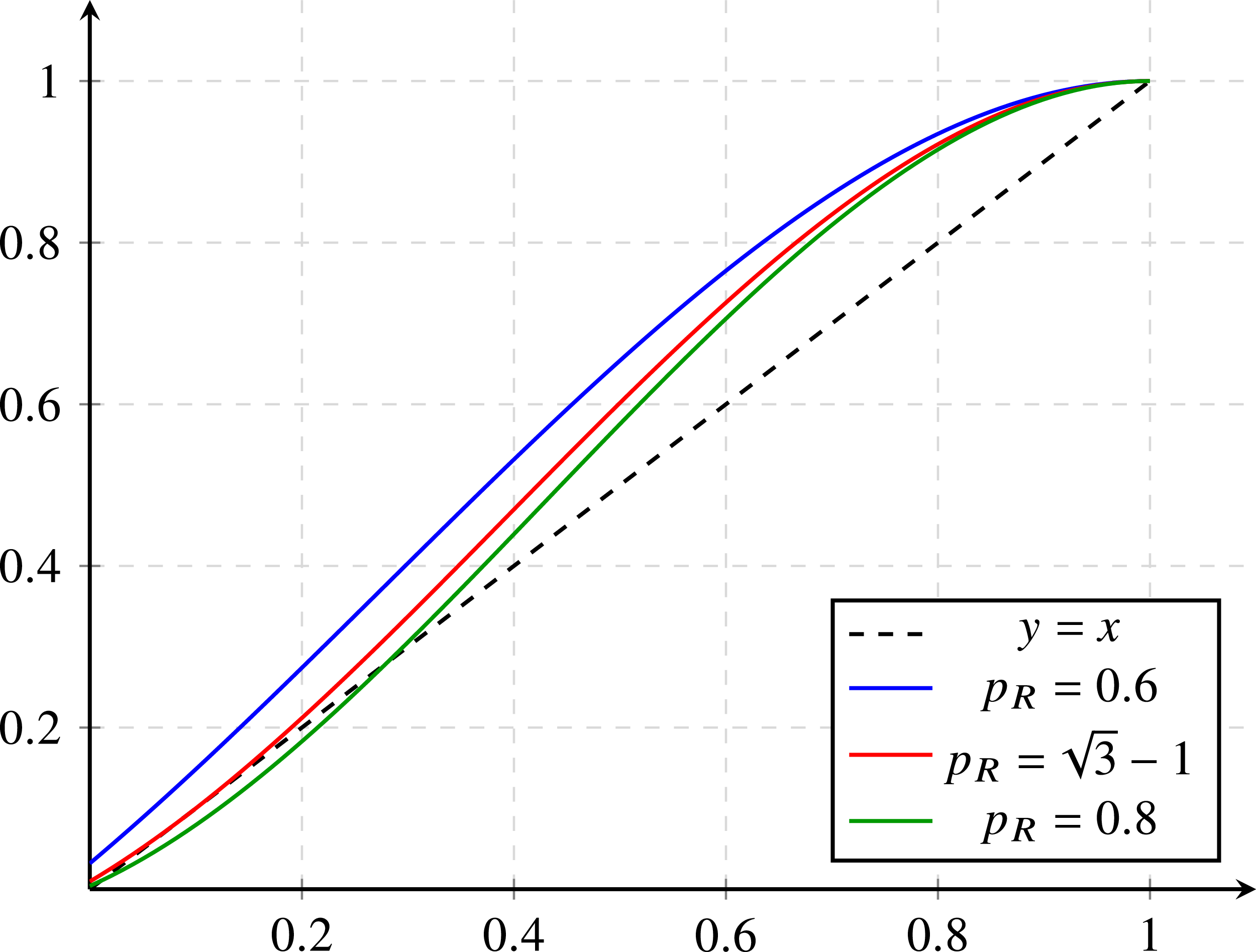
 y=g3(x)
 pR
 y=x
 [0,1]×[0,1]
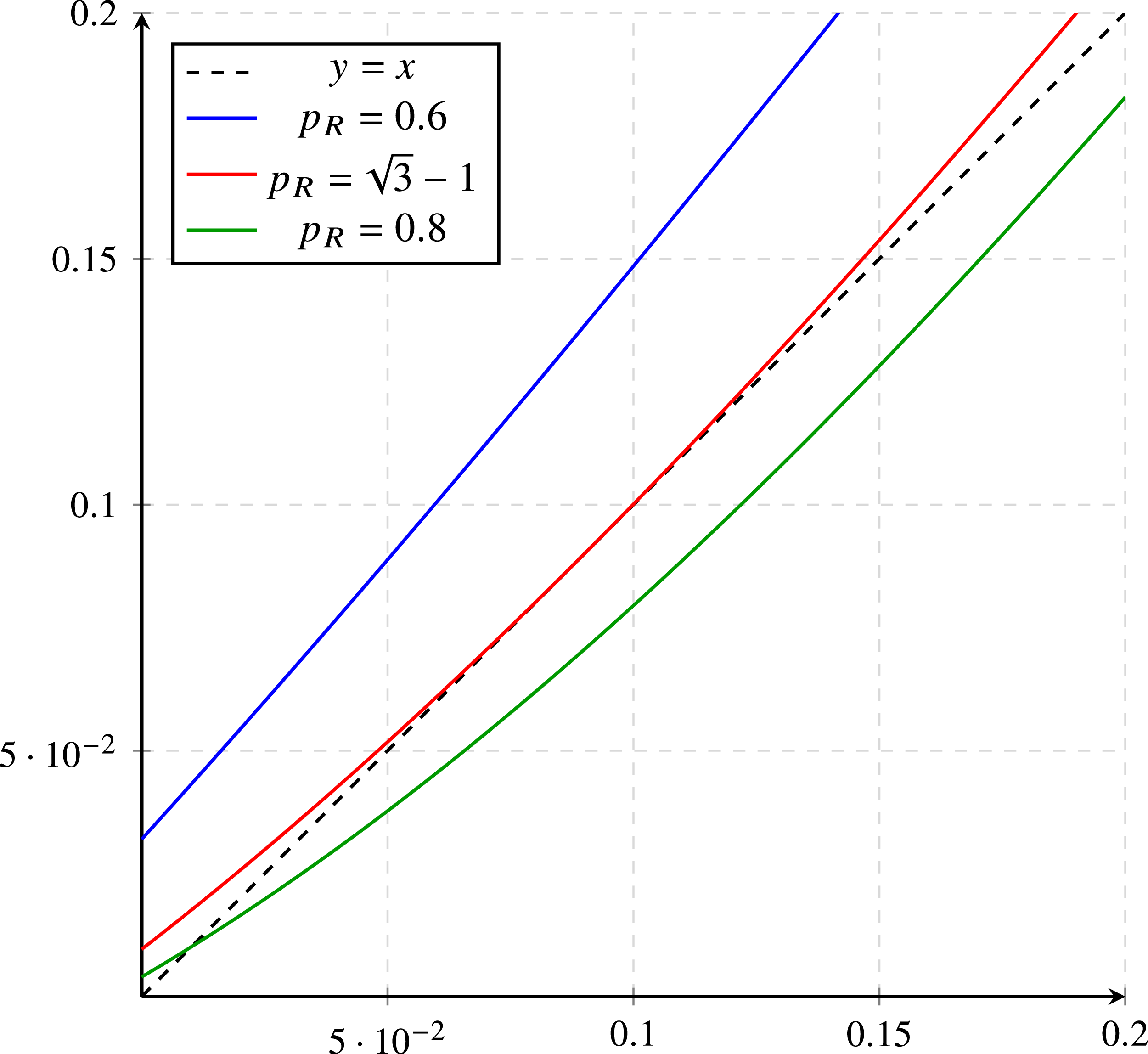
 y=g3(x)
 pR
 y=x


