2.1 Full spatio-temporal POD

Owing to the homogeneity of the statistics in the spatial directions $x$ and $z$ and their stationarity, POD modes are Fourier modes in the horizontal directions as well as in time (Berkooz et al. Reference Berkooz, Holmes and Lumley1993). Here, for each configuration, the Fourier transform of the velocity is computed in the temporal and the homogeneous spatial directions for each sample corresponding to a set of fields. The $p$ th component of the velocity field ( $u^{p}(x,y,z,t)$ ) in the physical space is then written as

(2.1) $$\begin{eqnarray}u^{p}(x,y,z,t)=\mathop{\sum }_{l}\mathop{\sum }_{k}\mathop{\sum }_{f}u_{lkf}^{p}(y)\text{e}^{2\unicode[STIX]{x03C0}\text{i}(lx/L_{x}+kz/L_{z}+ft/T)},\end{eqnarray}$$

where $u_{lkf}^{p}(y)$ denotes the $p$ th velocity component in the Fourier space corresponding to the streamwise wavenumber $l$ , spanwise wavenumber $k$ and frequency $f$ . Proper orthogonal decomposition is then applied in the wall-normal direction for each triad $(l,k,f)$ :

(2.2) $$\begin{eqnarray}u_{lkf}^{p}(y)=\mathop{\sum }_{n}a_{lkf}^{n}\unicode[STIX]{x1D719}_{lkf}^{n,p}(y),\end{eqnarray}$$

with, for any two $4$ -tuples $(l,k,f,n)$ and $(l,k,f,m)$ ,

(2.3) $$\begin{eqnarray}\langle a_{lkf}^{n}a_{lkf}^{m\ast }\rangle =\unicode[STIX]{x1D6FF}_{nm}\unicode[STIX]{x1D706}_{lkf}^{n}.\end{eqnarray}$$

Here, $\langle \cdot \rangle$ represents the usual ensemble average over the space of all possible flow realizations, $\unicode[STIX]{x1D6FF}_{mn}$ is the Kronecker-delta function, $n$ denotes a specific POD mode for each triad and * denotes complex conjugation. Note that $a_{lkf}^{n}$ is independent of $p$ as the three velocity components are stacked into a single vector. The complex, stochastic coefficients $a_{lkf}^{n}$ are uncorrelated and their variance is equal to $\unicode[STIX]{x1D706}_{lkf}^{n}$ .

Figure 1.

Schematic of the methodology. Each grey slab on the left represents an instantaneous realization of the flow in the physical domain (the wall-normal direction corresponding to the thickness of the slab), while each slab on the right corresponds to the Fourier transform of a block of $n_{t}$ realizations in time as well as in the horizontal directions $x$ and $z$ . For each Fourier triad $(l,k,f)$ the autocorrelation tensor is computed by averaging over the $N_{s}$ blocks and an independent eigenproblem is solved.

The eigenfunctions $\unicode[STIX]{x1D719}_{lkf}^{n,p}$ and eigenvalues $\unicode[STIX]{x1D706}_{lkf}^{n}$ are obtained by solving the following eigenproblem, where the autocorrelation is estimated from taking an ensemble average:

(2.4) $$\begin{eqnarray}\int _{0}^{Y}\langle \boldsymbol{u}_{lkf}(y)\boldsymbol{u}_{lkf}^{\ast }(y^{\prime })\rangle \unicode[STIX]{x1D753}_{lkf}^{n}(y^{\prime })\,\text{d}y^{\prime }=\unicode[STIX]{x1D706}_{lkf}^{n}\unicode[STIX]{x1D753}_{lkf}^{n}(y).\end{eqnarray}$$

Here, $\boldsymbol{u}_{lkf}(y)$ represents the single velocity vector with the three components stacked in it. Upon discretization in $y$ , $\unicode[STIX]{x1D753}_{lkf}^{n}(y)$ represents the single eigenvector containing the three components. By construction, the eigenvectors are orthonormal with respect to the Euclidean inner product, and $\unicode[STIX]{x1D706}_{lkf}^{n}$ can be interpreted as the energy content in each mode. Similarly, for each triad $(l,k,f)$ , the modes (i.e. different values of $n$ ) are sorted by energy. Since the left-hand side of (2.4) is a Hilbert–Schmidt integral operator, its eigenvalues are real and non-negative. The eigenvalues $\unicode[STIX]{x1D706}_{lkf}^{n}$ associated with the triplets $(l,k,f)$ can then be gathered and sorted globally according to their magnitude. We will call mode number the global index $N(l,k,f,n)$ associated with the sorted modes over spatial wavenumbers $(l,k)$ , frequency $(f)$ and quantum number $n$ , with lower mode number indicating a larger eigenvalue. In all that follows, we focus only on the most energetic modes.

2.2 Numerical implementation

The methodology is summarized in figure 1. Since POD is also applied in time, the autocorrelation tensor needs to be computed from several independent realizations of the same experiment. An ideal sample would consist of the Fourier transform in space and time of the velocity field corresponding to different databases obtained at the same Reynolds number. In practice, owing to the cost of the simulation, we split a single database into several contiguous chunks of length $T$ , each of which constitutes a sample. The samples are therefore not independent realizations, but we assume that the period $T$ is sufficiently larger than the characteristic time scales of the flow, or at least sufficiently large to allow separation of the dominant time scales. Yet $T$ cannot be too large in order to allow for a reasonable number of samples $N_{s}$ to be constituted. We note that as in Moin & Moser (Reference Moin and Moser1989) and Podvin (Reference Podvin2001), the number of samples is doubled by considering spanwise reflections and quadrupled by considering both lower and upper parts of the channel (including spanwise reflections).

Each sample then consists of a block of $n_{t}$ velocity fields uniformly sampled at a rate $\unicode[STIX]{x1D6FF}t$ . The value of $\unicode[STIX]{x1D6FF}t$ is chosen such that the Nyquist frequency is well above the range of characteristic frequencies of the flow. It is however limited by computational tractability, as large values of $n_{t}$ will increase memory requirements for the samples. For most of the test cases, we have fixed the value of $T$ to be 3000 wall units.

We use the finite-volume code SUNFLUIDH to simulate the incompressible flow in a channel. Further details of the configuration and numerical scheme can be found in Podvin & Fraigneau (Reference Podvin and Fraigneau2014). Periodic boundary conditions are enforced in the streamwise ( $x$ ) and the spanwise ( $z$ ) direction, and the channel lengths along these directions are $L_{x}=2\unicode[STIX]{x03C0}h$ and $L_{z}=\unicode[STIX]{x03C0}h$ , where $h$ is the channel half-height. The total domain is discretized using a grid of size $256\times 256\times 256$ , with a uniform grid for the horizontal directions $x$ and $z$ and a hyperbolic tangent-distributed mesh for the wall-normal direction $y$ . The velocity components in the streamwise, wall-normal and spanwise directions will be denoted, respectively, by $u$ , $v$ and $w$ or equivalently by $u_{1}$ , $u_{2}$ and $u_{3}$ . The simulation is conducted at $Re_{\unicode[STIX]{x1D70F}}=590$ , based on the friction velocity $u_{\unicode[STIX]{x1D70F}}$ and channel half-height $h$ , which corresponds to the simulation of Moser, Kim & Mansour (Reference Moser, Kim and Mansour1999). The database consists of 16 500 flow realizations, separated by $\unicode[STIX]{x1D6FF}t_{+}=5.9$ . The time spanned by the database represents about $10^{5}$ viscous time units.

In most of the paper, we focus on the domain $y_{+}<Y_{+}=80$ , but we also considered the full boundary layer where $Y_{+}=590$ . Due to the strong decrease of the energy spectra with the streamwise wavenumber, and given the typical extent of longitudinal streaks in the wall layer (about 600–1000 wall units (Jiménez Reference Jiménez2013)), the streamwise extent of the domain was limited to $L_{x}=\unicode[STIX]{x03C0}/2h$ representing 900 wall units. The full spanwise extent of the domain (about 1800 wall units) was considered.

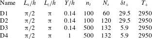
Results are reported for four datasets extracted from the single database, which represent different domain sizes and sampling rates. The characteristics of the different configurations are given in table 1. The sampling rate and number of samples were varied in the configurations D1–D3. These datasets correspond to the wall layer, $Y_{+}=80$ . The fourth one (D4) corresponds to the full boundary-layer height, $Y_{+}=590$ .

Table 1.

Description of different test cases; $n_{t}$ denotes the number of snapshots in a given block, $N_{s}$ denotes the number of samples, $\unicode[STIX]{x1D6FF}t_{+}$ is the time gap between successive snapshots and $T_{+}$ is the total time period for a given block (expressed in viscous units).

3.1 Snapshot POD

Snapshot POD (Sirovich Reference Sirovich1987) relies on an ergodicity assumption to identify the ensemble average operator $\langle \cdot \rangle$ with the time average. In practice, one has to rely on a finite set of samples (snapshots) and the average operator reduces to an empirical algebraic average. Snapshot POD then considers the empirical spatial autocorrelation tensor $\unicode[STIX]{x1D646}_{U}(\boldsymbol{x},\boldsymbol{x}^{\prime })=n_{t}^{-1}\sum _{j=1}^{n_{t}}u(\boldsymbol{x},t_{j})u(\boldsymbol{x}^{\prime },t_{j})$ , with $\boldsymbol{x}$ the vector-valued continuous space variable. Autocorrelation tensor eigenfunctions $\unicode[STIX]{x1D719}_{j}(\boldsymbol{x})$ , associated with the largest eigenvalues $\unicode[STIX]{x1D706}_{j}$ , are the dominant POD modes. The operator involved in the Fredholm equation of the snapshot POD method being Hilbert–Schmidt, its eigenfunctions are orthonormal with respect to the retained inner product.

The spatial autocorrelation tensor $\unicode[STIX]{x1D646}_{U}$ is estimated from a finite set of samples and then only provides an approximation of the true autocorrelation tensor $\unicode[STIX]{x1D646}_{U}^{\star }(\boldsymbol{x},\boldsymbol{x}^{\prime })=\text{lim}_{|\unicode[STIX]{x1D6FA}_{t}|\rightarrow \infty }|\unicode[STIX]{x1D6FA}_{t}|^{-1}\int _{\unicode[STIX]{x1D6FA}_{t}}u(\boldsymbol{x},t)u(\boldsymbol{x}^{\prime },t)\,\text{d}t$ . In general, the spatial POD modes are then only an approximation of the true autocorrelation eigenvectors. In the spatio-temporal POD approach, we take advantage of the closed-form solution of the Fredholm equation in homogeneous dimensions. No approximation is then introduced and the spatio-temporal modes are the exact eigenvectors of the autocorrelation tensor along the homogeneous dimensions.

From a dynamical perspective, the temporal evolution of snapshot POD mode $j$ is given by the orthogonal projection of the flow field onto the corresponding eigenfunction: $a_{j}(t)=(\unicode[STIX]{x1D719}_{j},\boldsymbol{u}(t))$ , where $\boldsymbol{u}(t)\equiv u(\boldsymbol{x},t)$ and $(,)$ represents the (typically weighted Euclidean) inner product. The time evolution of mode $j$ then inherits many properties of the flow field such as its wide frequency content. It is important to note that, since it results from a projection, there is no guarantee that the dynamics of a snapshot POD mode is smooth in time.

In contrast, the present spatio-temporal POD relies on a spectral decomposition in the homogeneous dimensions, including time. Each mode then follows a smooth (harmonic) dynamics. The original flow field being approximated by a finite linear combination of smooth modes, it remains smooth in time. More generally, spatio-temporal POD enjoys structure in both time and homogeneous dimensions and allows one to interpret modes as coherent structures, localized in the frequency–spatial wavenumber space. In contrast, snapshot POD only enjoys structure in space and lacks structure in time, preventing identification of its modes with coherent structures the dynamics of which is essentially smooth.

3.2 Dynamic mode decomposition

The DMD is another popular method for modal decomposition of fluid flows. Different definitions have been considered in the literature but we here focus on the original formulation discussed in Schmid (Reference Schmid2010). Considering the flow field at a collection of $N_{x}$ points in space as a vector-valued observable, and assuming it is a state vector for the underlying physical system, the DMD can be closely related to the Koopman theory, Mezić (Reference Mezić2005), Rowley et al. (Reference Rowley, Mezić, Bagheri, Schlatter and Henningson2009). In a nutshell, the DMD estimates the eigenvectors and associated eigenvalues of the linear operator mapping the discrete flow field at a given time to a subsequent time $\unicode[STIX]{x0394}t$ in the future. Specifically, $n_{t}$ time-ordered snapshots of the flow field sampled every $\unicode[STIX]{x0394}t$ in time are collected in a matrix $\unicode[STIX]{x1D650}$ . Each snapshot is of size $N_{x}$ and constitutes a vector-valued observable $\boldsymbol{u}$ of the state vector of the underlying physical system. Letting $U_{1}$ be the first $n_{t}-1$ columns of $\unicode[STIX]{x1D650}$ and $U_{2}$ the last $n_{t}-1$ columns, the DMD is concerned with the characterization of the linear operator $A$ such that $U_{2}\simeq AU_{1}$ . Formulating the approximation as an optimization problem, the eigendecomposition of the matrix $\unicode[STIX]{x1D63C}$ can be obtained: $A\unicode[STIX]{x1D6F9}=\unicode[STIX]{x1D6F9}\unicode[STIX]{x1D6EC}$ , with $\unicode[STIX]{x1D6F9}\in \mathbb{C}^{(n_{t}-1)\times (n_{t}-1)}$ the matrix of eigenvectors and $\unicode[STIX]{x1D6EC}\in \mathbb{C}^{(n_{t}-1)\times (n_{t}-1)}$ the diagonal matrix of eigenvalues $\unicode[STIX]{x1D706}_{j}$ . The flow field $u\left(\boldsymbol{x},t\right)$ is identified with $\boldsymbol{u}(t)$ and can then be approximated at a time $t+l\unicode[STIX]{x0394}t$ as

(3.1) $$\begin{eqnarray}\boldsymbol{u}(t+l\unicode[STIX]{x0394}t)\approx \unicode[STIX]{x1D6F9}\,\text{diag}(\unicode[STIX]{x1D6F9}^{-1}\boldsymbol{u}(t))\unicode[STIX]{x1D740}^{l}=\unicode[STIX]{x1D6EF}\unicode[STIX]{x1D740}^{l},\quad \forall \,l\in \mathbb{Z},\end{eqnarray}$$

where $\unicode[STIX]{x1D740}^{l}=(\unicode[STIX]{x1D706}_{1}^{l}\unicode[STIX]{x1D706}_{2}^{l}\cdots \unicode[STIX]{x1D706}_{n_{t}-1}^{l})^{\text{T}}$ and the matrix $\unicode[STIX]{x1D6EF}=(\unicode[STIX]{x1D743}_{1}\unicode[STIX]{x1D743}_{2}\cdots \unicode[STIX]{x1D743}_{n_{t}-1})$ contains the so-called DMD modes $\unicode[STIX]{x1D743}_{j}$ .

Assuming the collection of snapshots is linearly independent and subtracting the empirical algebraic time average from the snapshot data $\unicode[STIX]{x1D650}$ , the DMD is equivalent to the temporal discrete Fourier transform (Chen, Tu & Rowley Reference Chen, Tu and Rowley2012). Specifically, denoting zero-mean quantities with a superscript $^{\odot }$ , the vector-valued observable $\boldsymbol{u}^{\odot }(t+l\unicode[STIX]{x0394}t)$ then obeys

(3.2) $$\begin{eqnarray}\boldsymbol{u}^{\odot }(t+l\unicode[STIX]{x0394}t)=\mathop{\sum }_{j=1}^{n_{t}-1}\exp \left(\frac{2\unicode[STIX]{x03C0}\text{i}lj}{n_{t}}\right)\unicode[STIX]{x1D743}_{j}.\end{eqnarray}$$

In this context, DMD decomposes the flow field in monochromatic spatial modes $\unicode[STIX]{x1D743}_{j}$ oscillating at a given frequency $j/(\unicode[STIX]{x0394}tn_{t})$ in time. Both the spatio-temporal POD and DMD then derive modes oscillating at a given frequency. The sampling frequency being a multiple integer of these frequencies, both methods represent the data with modes at the same frequencies.

However, an essential difference between DMD and POD is that there is no notion of ensemble average in DMD (only one sample, corresponding to the set of snapshots, is considered), and DMD modes are extracted from mapping one snapshot in the time series to the next one. Standard DMD is applied to one flow realization, and thus a mode computed at given frequency would have statistical variability over a set of realizations. In contrast, in the present decomposition, ensemble average is a key feature of the procedure and requires several samples. The POD modes are extracted from the autocorrelation tensor built from the different samples. They constitute an optimal basis that accounts for the variability of modes over an ensemble of realizations. We point out that in our numerical implementation, the different samples are obtained by breaking down a single series of snapshots into different non-overlapping blocks.

3.3 Requirements and cost of the decomposition

The spatio-temporal POD discussed in this paper relies on the same information as the snapshot POD or the DMD. Owing to the discrete Fourier transform in time and homogeneous spatial directions, it however involves distinctive differences such as the requirement of collecting time-resolved snapshots. This is in contrast with the other methods which only require time-sampling in pairs (DMD) or a set of snapshots sampled in time according to an approximately ergodic measure (snapshot POD).

Obtaining time-resolved data in the full spatial domain from a numerical simulation is not a problem, but requires integration over a sufficiently long period of time, especially if it needs to be broken down into different samples. In contrast, in an experiment, obtaining different samples over relatively long periods of time is relatively easy, but access to full spatial resolution may be more difficult, especially for time-resolved data, despite recent advances in particle image velocimetry techniques (see for instance Westerwheel, Elsinga & Adrian Reference Westerwheel, Elsinga and Adrian2013). However, it should be borne in mind that ensemble average and Fourier transform commute, so that full information in the spatial domain does not have to be acquired simultaneously, since the autocorrelation tensor for given spatial separations in homogeneous directions can be computed independently. If there is one homogeneous direction (say $x$ ), the autocorrelation tensor $\unicode[STIX]{x1D646}_{U}(x_{1},y_{1},x_{2},y_{2})=f(x_{2}-x_{1},y_{1},y_{2})$ can be evaluated independently for each separation $x_{2}-x_{1}$ from two simultaneous planes $x=x_{1}$ and $x=x_{2}$ : the information does not have to be acquired for all positions $x$ at the same time, only pairs of simultaneous positions are necessary. For the same reason, in the case of two homogeneous directions ( $x$ and $z$ ), one can show that the full spatial autocorrelation tensor at all separations $(x_{1}-x_{2},z_{1}-z_{2})$ can be entirely recovered from two orthogonal planes $x=\text{cst}$ and $z=\text{cst}$ (as was done in the WALLTURB experiment (Stanislas, Jimenez & Marusic (Reference Stanislas, Jimenez and Marusic2011))).

We now briefly discuss the numerical cost of the solution method presented in this paper. We consider the common situation where the sampling is uniform in time and sufficiently finely resolved with respect to the finest scales in which one is interested. A discrete Fourier transform is then applied in homogeneous dimensions. We use a multidimensional fast Fourier transform which essentially amounts to the composition of a sequence of one-dimensional fast Fourier transforms along each homogeneous dimension. The numerical cost of this step then retains the $O(N\log (N))$ scaling of fast Fourier transform techniques, where $N$ is here $N_{l},N_{k}$ or $n_{t}$ . Efficient algorithms also exist in the case of non-uniform sampling (e.g. Ruiz-Antolín & Townsend (Reference Ruiz-Antolín and Townsend2018)), and retain the $O(N\log (N))$ scaling. The remaining step involves a POD in the non-homogeneous dimension for each atom of triad $(l,k,f)$ . In the present case, it then reduces to a set of independent one-dimensional PODs.

Finally, we stress that the eigenvalue problems involved in every method discussed here (spatio-temporal POD, spatial POD, DMD) can be advantageously solved by recent numerical techniques. In particular, sketching and randomized methods (Halko, Martinsson & Tropp Reference Halko, Martinsson and Tropp2011; Kannan & Vempala Reference Kannan and Vempala2017) can very significantly alleviate the numerical cost and the memory requirement in cases where only part of the spectrum is required, as is often the case in our applications.

4.1 Proper orthogonal decomposition eigenvalues

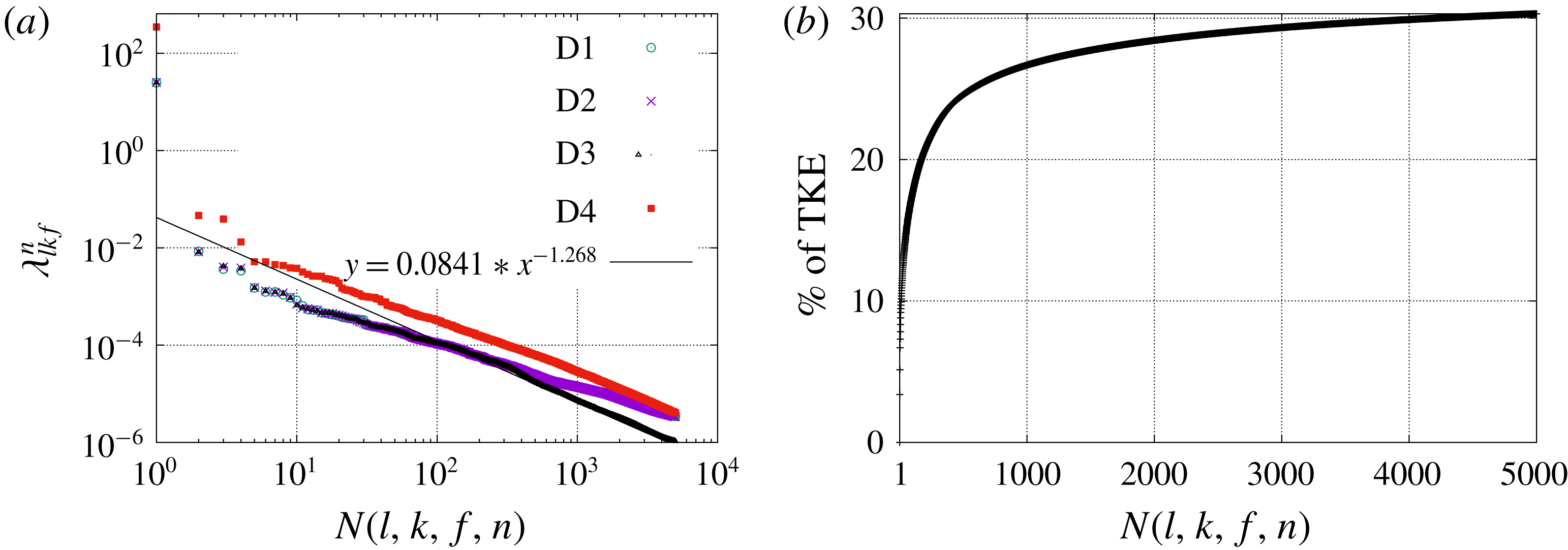
Figure 2(a) shows the top 5000 eigenvalues for each configuration. We note that this represents a tiny fraction of the total number of eigenvalues defined in the spatio-temporal space, which is $3n_{t}\times N_{l}\times N_{k}\times N_{y}$ , where $n_{t}$ is the number of instantaneous fields contained in a sample, $N_{l}$ and $N_{k}$ are, respectively, the numbers of streamwise and spanwise wavenumbers and $N_{y}$ is the number of grid points in the wall-normal direction. For D3 this corresponds to about $4\times 10^{8}$ degrees of freedom. The largest eigenvalue $N(l,k,f,n)=1$ , where $l=k=f=0$ and $n=1$ , corresponds to that of the mean mode (discussed in the next section). For each configuration, we have applied spatio-temporal POD to the data without removing the sample mean and compared the results to the case where the sample mean was removed. In both cases the eigenvalue distribution was very similar, and the deviations in eigenfunctions were negligibly small at least for the most energetic modes. In the rest of the paper we will focus on the $n=1$ eigenfunctions. We note that the eigenfunctions corresponding to $n=1$ capture about $80\,\%$ of the TKE, which is in agreement with the results of Moin & Moser (Reference Moin and Moser1989).

Figure 2.

(a) Log–log plot of the top 5000 eigenvalues for D1–D4 configurations. An asymptotic fit for the decay rate of the spectra for D3 is also shown. (b) Percentage of TKE captured by the $N$ most energetic modes for D3.

Figure 2(a) shows that the spectrum eigenvalues in D1 and D2, which correspond to a different number of samples, are essentially indistinguishable from each other. This indicates that the number of samples of ensemble averaging appears to be sufficient for the convergence of the dominant eigenvalues. The eigenvalues in D1 and D2 are similar to that in D3 at low values of $N$ , but have higher energy levels at large values of $N$ , which is likely to be due to aliasing effects as the fields are sampled at higher rates there than in D3. The spectrum has an asymptotic decay of $\unicode[STIX]{x1D706}(N)\sim N^{-1.27}$ . Unlike the other configurations, D4 corresponds to the full boundary layer $0<y_{+}<590$ . As expected, energy levels are higher but the shape of the spectrum and its asymptotic decay rate are the same as in the wall region $0<y_{+}<80$ , which suggests self-similarity (see next section). Figure 2(b) shows the fraction of TKE captured by the first $N$ modes for each $N$ (as we are considering fluctuations, the contribution from the mean mode was set to zero). The fraction of TKE captured by the most energetic $100$ mode numbers is relatively high, but increases only slightly for mode numbers higher than $1000$ , which highlights the complexity of the flow. The slow convergence in Fourier space also indicates that the structures are highly localized in space and time, owing to the fundamentally intermittent nature of turbulence (Frisch Reference Frisch1995). This is confirmed by table 2, which shows that the first $200$ eigenvalues capture about $21\,\%$ of the TKE which is increased only to $32\,\%$ when $5000$ modes are included, for the D3 configuration. The trend remains the same for the D4 configuration, where $200$ eigenvalues capture around $24\,\%$ of TKE which increases only to $34\,\%$ when $5000$ eigenvalues are included.

Figure 3.

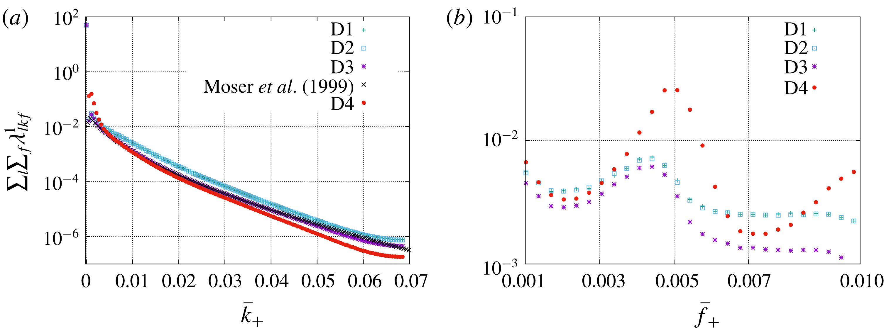
(a) Integrated energy spectrum ( $\sum _{l}\sum _{f}\unicode[STIX]{x1D706}_{lkf}^{1}$ ) as a function of $\bar{k}_{+}$ ; the data are compared with the energy spectrum of Moser et al. (Reference Moser, Kim and Mansour1999) at $y_{+}=80$ (with appropriate rescaling). (b) Integrated energy spectrum ( $\sum _{l}\sum _{k}\unicode[STIX]{x1D706}_{lkf}^{1}$ ) as a function of $\bar{f}_{+}$ for $0<y_{+}<80$ (D1–D4).

Table 2.

Percentage of TKE in the first $N$ eigenvalues for D3 and D4 configurations.

Figure 3 shows the dependence of the integrated spectra with respect to the frequency and spanwise wavenumber for the different configurations. For the D3 configuration, the spatial wavenumbers and the frequency $(\bar{l},\bar{k},\bar{f})$ , expressed in wall units, are related to the mode indices $(l,k,f)$ as

(4.1a-c ) $$\begin{eqnarray}\bar{l}_{+}=\frac{l}{927},\quad \bar{k}_{+}=\frac{k}{1854},\quad \bar{f}_{+}=\frac{f}{2950}.\end{eqnarray}$$

Figure 3(a) shows how the sum of the eigenvalues over streamwise wavenumber and frequencies ( $\sum _{l}\sum _{f}\unicode[STIX]{x1D706}_{lkf}^{1}$ ) varies as a function of $\bar{k}_{+}$ . Results show a good agreement with the rescaled standard energy spectrum obtained by Moser et al. (Reference Moser, Kim and Mansour1999) at $y_{+}=80$ . As expected, the spanwise spectrum over the full layer has more energy in the lower wavenumbers and less energy at higher wavenumbers compared to that in the wall layer.

Figure 3(b) shows the sum of the dominant $n=1$ eigenvalues over all $(l,k)$ modes (i.e.  $\sum _{l}\sum _{k}\unicode[STIX]{x1D706}_{lkf}^{1}$ ) as a function of frequency $\bar{f}_{+}$ for the different configurations D1–D4. As observed previously, aliasing effects can be observed for the fields sampled in time at a lower rate (D1 and D2), but the trends are very similar. A marked increase in the energy is observed in the frequency range of $0.003{-}0.005$ , which corresponds to time scales of 200–300 viscous units. This value is in good agreement with the duration of the regeneration cycle identified by Hamilton et al. (Reference Hamilton, Kim and Waleffe1995) and Jimenez & Moin (Reference Jimenez and Moin1991) in minimal domains, as well as the investigations of larger-scale domains reported in Jiménez (Reference Jiménez2013). A similar frequency peak is observed in the full boundary layer (D4), but with a shift towards slightly higher frequencies: the maximum is located at $\bar{f}_{+}=0.005$ , while it is located at $\bar{f}_{+}=0.0044$ , in the region $y_{+}<80$ .

As far as we know, this is the first evidence of an objective time scale identified in the channel configuration. The time scale did not appear to be affected by spatial variability: it did not depend on the spanwise extent (different domain widths were considered) or the streamwise extent of the domain (two domains of different streamwise sizes were compared). We note that the dominant frequency of the nonlinear terms (e.g. the Reynolds stresses) should be of the order of 100–150 wall units. An interesting connection, which will need further exploration, can be made with wall reduction control schemes based on wall spanwise oscillations such as those of Choi, Debisschop & Clayton (Reference Choi, Debisschop and Clayton1998) and Quadrizio & Ricco (Reference Quadrizio and Ricco2004), where it was shown that the optimal oscillation period is about 100–150 wall units.

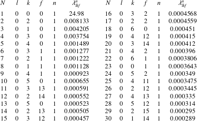
The predominance of the characteristic frequency $\bar{f}_{c+}$ at $\bar{f}_{+}=0.0044$ is confirmed by table 3, which shows the top 30 eigenvalues (denoted by $\unicode[STIX]{x1D706}_{lkf}^{n}$ ) with the corresponding Fourier mode indices $(l,k,f)$ in space and time and quantum mode $n$ for configuration D3. Although a large fraction (18 modes) of the first 30 modes are associated with $f\leqslant 2$ , which corresponds to long time scales that are outside the scope of our analysis, all the other modes are characterized by frequencies between $11$ and $15$ , which correspond to the previously identified time scale of about 200–300 viscous units. The most energetic of these modes corresponds to $f=13$ , i.e.  $\bar{f}_{c+}$ . We note that all the modes in the table are characterized by $n=1$ , which corresponds to the largest eigenvalue for a triad $(l,k,f)$ , and $l=0$ , which corresponds to the streamwise-averaged flow.

Table 3.

Top 30 most energetic eigenvalues $\unicode[STIX]{x1D706}_{lkf}^{n}$ along with their corresponding $(l,k,f,n)$ .

Figure 4.

Horizontally averaged ( $x$ and $z$ ) temporal Fourier transform of the streamwise velocity component $u$ as a function of $\bar{f}_{+}$ in a log–log scale at (a) $y_{+}=3$ and (b) $y_{+}=15$ . A vertical line is shown at $\bar{f}_{+}=0.005$ to indicate the peak in both panels.

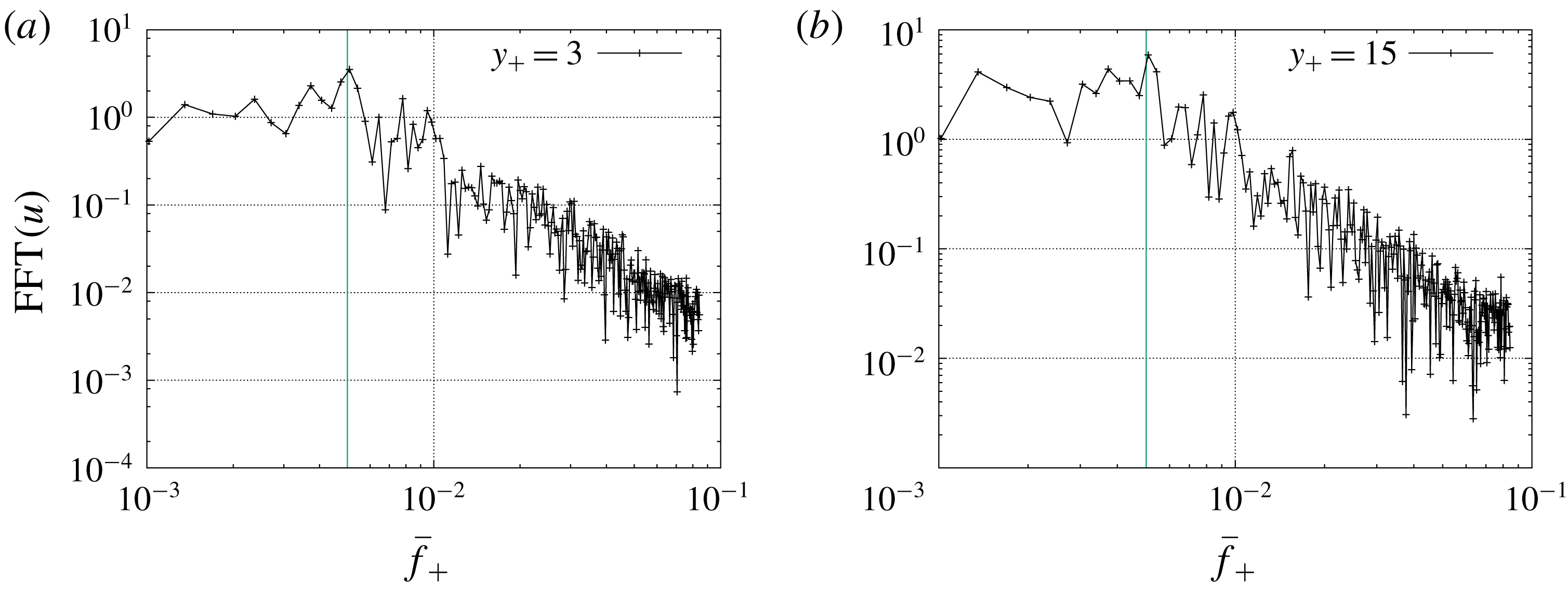
To provide a comparison with standard analysis tools, figure 4(a,b) shows the temporal Fourier transform of the streamwise velocity component averaged along horizontal directions for two different heights: $y_{+}=3$ and $15$ . Although there seems to be some energy increase around the characteristic frequency $\bar{f}_{c+}$ , evidence of a local peak is not clear in this figure. This illustrates the usefulness of the new POD implementation.

Figure 5.

Eigenvalue distribution of the top 5000 eigenvalues for D3 configuration as a function of (a) $\bar{f}_{+}$ and (b) $\bar{k}_{+}$ .

Figure 6.

(a) Energy spectrum (represented in log scale) summed over frequency $f$ , $\sum _{f}\unicode[STIX]{x1D706}_{lkf}^{1}$ , for different streamwise wavenumbers $l$ as a function of $\bar{k}_{+}$ . (b) Energy spectrum (represented in log scale) summed over spanwise wavenumber $k$ , $\sum _{k}\unicode[STIX]{x1D706}_{lkf}^{1}$ , for different streamwise wavenumbers $l$ as a function of $\bar{f}_{+}$ .

Figures 5(a) and 5(b), respectively, show the distribution of the top 5000 eigenvalues along $\bar{k}_{+}$ and $\bar{f}_{+}$ for the D3 configuration. Each eigenvalue is represented by a dot. Both figures show that the peaks observed in frequency and wavenumber space are not created by an accumulation of small eigenvalues, but correspond to coherent, more energetic structures. We note that figure 5(b) also shows smaller, but noticeable peaks of $\bar{f}_{+}$ at around 0.009 and 0.0135, which correspond to the harmonics of the frequency $0.0044$ .

Figure 6(a) shows that the energy spectrum integrated in frequency space $\sum _{f}\unicode[STIX]{x1D706}_{lkf}^{1}$ slowly decreases in an apparently self-similar manner with respect to both streamwise and spanwise wavenumbers. Figure 6(b) shows the corresponding variations in the frequency space of the energy spectrum integrated in the spanwise wavenumber space for different streamwise wavenumbers $l$ . For the $l=0$ mode, owing to spanwise reflection invariance, the plot is symmetric in the frequency space, and the characteristic frequency $\bar{f}_{c+}$ and its harmonics can be clearly identified. These peaks observed at $l=0$ are still present in the $l\neq 0$ spectra, which confirms that the characteristic frequency $f_{c+}$ is not an artifact of the streamwise average. However non-zero streamwise wavenumbers are also characterized by a broad peak, which represents convection effects. In general, defining a convection velocity for the turbulent wall layer is not straightforward (Krogstad, Kaspersen & Rinestead Reference Krogstad, Kaspersen and Rinestead1998; Alamo & Jimenez Reference Alamo and Jimenez2009), but the question can be more easily addressed in the present framework where each POD eigenfunction is naturally associated with a phase velocity $-\bar{f}/\bar{l}$ . The spectra $\sum _{k}\unicode[STIX]{x1D706}_{lkf}^{1}$ can be used to define a global convection velocity $c$ at each streamwise wavenumber using

(4.2) $$\begin{eqnarray}c(\bar{l})=-\frac{\bar{f}_{max}}{\bar{l}},\end{eqnarray}$$

where

(4.3) $$\begin{eqnarray}\bar{f}_{max}=\text{arg}\,\text{max}_{\bar{f}}\left[\mathop{\sum }_{k}\unicode[STIX]{x1D706}_{lkf}^{1}\right].\end{eqnarray}$$

Peaks in the spectra are located at $\bar{f}_{+}=(0.013,0.027,0.044)$ for respective streamwise wavenumbers of $\bar{l}_{+}=(0.0011,0.0022,0.0033)$ . This corresponds to a global convection velocity of 12 $u_{\unicode[STIX]{x1D70F}}$ , with a slight upward shift observed with increasing streamwise wavenumbers. This agrees well with the classical results (Kreplin & Eckelmann Reference Kreplin and Eckelmann1979; Krogstad et al. Reference Krogstad, Kaspersen and Rinestead1998; Alamo & Jimenez Reference Alamo and Jimenez2009; Wallace Reference Wallace2014).

Having access to four-dimensional space provides a way to test Taylor’s frozen turbulence hypothesis (Lumley Reference Lumley1965), which states that the spatial spectrum in the streamwise direction $E_{k_{x}}$ of $\overline{u(x)u(x^{\prime })}$ (where the overbar represents a spatial average) can be recovered from the temporal spectrum $E_{\overline{f}}$ of $\overline{\overline{u(t)u(t^{\prime })}}$ (the double overbar denotes here a temporal average) where $\overline{f}=kU$ and $U$ is a suitable convection velocity. In the context of the present decomposition, this leads us to compare, for each spanwise wavenumber $k_{z}$ and quantum mode $n$ , the temporal spectrum

(4.4) $$\begin{eqnarray}\tilde{E}(\overline{f},k_{z},n)=\mathop{\sum }_{l}\unicode[STIX]{x1D706}_{lkf}^{n}\unicode[STIX]{x1D6FF}k_{x},\end{eqnarray}$$

where $\overline{f}=f/T$ and $k_{z}=k/L_{z}$ , with the streamwise spectrum for the streamwise wavenumber $k_{x}$

(4.5) $$\begin{eqnarray}E(k_{x},k_{z},n)=\mathop{\sum }_{f}\unicode[STIX]{x1D706}_{lkf}^{n}\unicode[STIX]{x1D6FF}\overline{f},\end{eqnarray}$$

where $k_{x}=l/L_{x}$ , using a suitable rescaling factor $\unicode[STIX]{x1D6FF}k_{x}/\unicode[STIX]{x1D6FF}\overline{f}$ which can be obtained from

(4.6) $$\begin{eqnarray}{\mathcal{E}}=\mathop{\sum }_{l}\mathop{\sum }_{k}\mathop{\sum }_{f}\unicode[STIX]{x1D706}_{lkf}^{1}\unicode[STIX]{x1D6FF}k_{x}\unicode[STIX]{x1D6FF}k_{z}\unicode[STIX]{x1D6FF}\overline{f}=\mathop{\sum }_{l}\mathop{\sum }_{k}E(k_{x},k_{z},n)\unicode[STIX]{x1D6FF}k_{x}\unicode[STIX]{x1D6FF}k_{z}=\mathop{\sum }_{f}\mathop{\sum }_{k}\tilde{E}(f,k_{z},n)\unicode[STIX]{x1D6FF}\overline{f}\unicode[STIX]{x1D6FF}k_{z}.\end{eqnarray}$$

For the first quantum mode $n=1$ , figure 7 compares the spectrum in the temporal direction $E(k_{x},k_{z},1)$ with the equivalent spectrum in the streamwise direction $\tilde{E}(f,k_{z},1)$ . The frequency expressed in wall units $f_{+}$ is related to the the streamwise wavenumber $k_{x+}$ such that $k_{x+}U_{c+}=f_{+}$ , where we have taken $U_{c+}=12$ . For the range of corresponding frequencies, a good agreement can be observed between the spectra at each spanwise wavenumber $k_{z}$ .

Figure 7.

(a) Eigenvalue spectrum $\sum _{l}\unicode[STIX]{x1D706}_{lkf}^{1}\unicode[STIX]{x1D6FF}k_{x+}$ as a function of $f_{+}$ . (b) Eigenvalue spectrum $\sum _{f}\unicode[STIX]{x1D706}_{lkf}^{1}\unicode[STIX]{x1D6FF}k_{x+}$ as a function of $k_{x+}U_{c+}$ , where $U_{c+}=U=12$ . The colour bar is based on the decadic log scale.

4.2 Proper orthogonal decomposition eigenfunctions

Figure 8 shows that the reconstructed mean streamwise profile coincides with previous results (Moser et al. Reference Moser, Kim and Mansour1999) and with the dominant mode $(l=0,k=0,f=0,n=1)$ of the decomposition. Figure 9 shows the absolute value of each component of the most energetic mode $\unicode[STIX]{x1D719}_{lkf}^{p,n}$ , for $(\bar{l}_{+},\bar{k}_{+},\bar{f}_{+})=(0,0.0016,0.0044)$ , obtained for the datasets D1–D3. As expected, there is a good agreement between the different configurations, which indicates convergence of the procedure at least for the most energetic modes. In all that follows only results for D3 and D4 will be presented.

Figure 8.

Comparison of the mean streamwise profile reconstructed using the first eigenfunction for the mode pair $(0,0,0)$ with that of Moser et al. (Reference Moser, Kim and Mansour1999), and with the mean profile obtained from the direct numerical simulation.

Figure 9.

Comparison of the eigenfunctions $\unicode[STIX]{x1D753}_{lkf}^{1}$ corresponding to $\bar{l}_{+}=0$ , $\bar{k}_{+}=0.0016$ , $\bar{f}_{+}=0.0044$ for different configurations. (a) Streamwise component, (b) wall-normal component and (c) spanwise component.

In order to gain more insight into the structure of the modes, figure 10(a,c,e) shows the shape of the most energetic eigenfunction components $\unicode[STIX]{x1D753}_{0kf}^{1,p}$ associated with the characteristic frequency $\bar{f}_{c+}\sim 0.0044$ for different spanwise wavenumbers. The location of the velocity maxima moves closer to the wall as the spanwise wavenumber increases, which is in agreement with previous descriptions of wall-attached structures (Alamo et al. Reference Alamo, Jimenez, Zandonade and Moser2006; Podvin et al. Reference Podvin, Fraigneau, Jouanguy and Laval2010). The values of the maxima are similar for both cross-stream components, also in agreement with previous observations (Alamo et al. Reference Alamo, Jimenez, Zandonade and Moser2006; Podvin & Fraigneau Reference Podvin and Fraigneau2017), but the value tends to increase with the spanwise wavenumber for the streamwise and the wall-normal components, while it slightly decreases for the spanwise component. The monotonic evolution of the shape of the modes with the spanwise wavenumber suggests self-similarity, as was proposed in Podvin & Fraigneau (Reference Podvin and Fraigneau2017).

Figure 10(b,d,f) compares the eigenfunctions obtained on the domain $0<y_{+}<80$ (for D3) and $0<y_{+}<590$ (for D4) for several spanwise wavenumbers. The eigenfunctions of D4 have been rescaled to have the same energy content as those of D3 on $0<y_{+}<80$ . We observe that the eigenfunctions nearly coincide over their common definition domain, which is not a trivial result. The persistence of the eigenfunction shape with respect to the wall-normal extension of the decomposition domain shows the coherence of the most energetic motions over the entire height of the boundary layer. It also means that the restrictions of the eigenfunctions on the larger domain are orthogonal to each other on the smaller domain (since they coincide with the eigenfunctions there), which makes it possible to recover the amplitude of the eigenfunction on the larger domain directly from the projection of the velocity field in the smaller domain onto the corresponding eigenfunction. This shows the relevance of the decomposition for estimation purposes in a context of partial information (see for instance Podvin et al. Reference Podvin, Fraigneau, Jouanguy and Laval2010).

Figure 10.

Dominant eigenfunctions $\unicode[STIX]{x1D753}_{0kf}^{1}$ corresponding to $\bar{f}_{c+}$ and for increasing values of $\bar{k}_{+}$ . (a,b) Streamwise component. (c,d) Wall-normal component. (e,f) Spanwise component. (a,c,e) Comparison for $0<y_{+}<80$ (D3) and different spanwise wavenumbers ( $k=1$ to $8$ which correspond to $\bar{k}_{+}$ between $0.0011$ and $0.0086$ ). (b,d,f) Comparison between the domains $0<y_{+}<80$ (D3) and $0<y_{+}<590$ (D4) for selected wavenumbers $k=1,3,5,7$ .

Figure 11 shows the hierarchical organization of the eigenfunctions in various dimensions of four-dimensional space. For each streamwise wavenumber and quantum mode, we define the intensity of the eigenfunctions as a function of height and absolute frequency (for the sake of clarity positive and negative frequencies are aggregated, although as seen in a previous section there is no symmetry): $I_{ln}(y,|\overline{f}|)=\sum _{k}(\unicode[STIX]{x1D706}_{lkf}^{n}|\unicode[STIX]{x1D753}_{lkf}^{n}(y)|^{2}+\unicode[STIX]{x1D706}_{lk-f}^{n}|\unicode[STIX]{x1D753}_{lk-f}^{n}(y)|^{2}).$ This is represented in figure 11 for the first quantum numbers $n\leqslant 4$ and selected streamwise wavenumbers $l$ . Each quantum number $n$ is characterized by $n$ peaks at a given frequency. The wall-normal location of the highest peak increases nearly linearly with the quantum number $n$ , and is about $10n$ in wall units. At a given wavenumber in the horizontal space, energy is therefore transferred from the more energetic to the less energetic modes towards the core region away from the wall. The range of frequencies associated with a high intensity increases only slightly with the quantum number $n$ , but increases significantly with the streamwise wavenumber $l$ with a shift towards higher frequencies, which is due to convection effects.

Figure 11.

Structure intensity $I_{ln}(y,|\overline{f}|)=\sum _{k}\unicode[STIX]{x1D706}_{lkf}^{n}|\unicode[STIX]{x1D753}_{lkf}^{n}(y)|^{2}+\unicode[STIX]{x1D706}_{lk-f}^{n}|\unicode[STIX]{x1D753}_{lk-f}^{n}(y)|^{2}$ as a function of the vertical direction $y$ and of the frequency $|\overline{f}|$ for the first quantum numbers $n\leqslant 4$ and different streamwise wavenumbers $l$ . From left to right: increasing quantum numbers $n=1,2,3,4$ . From top to bottom: increasing streamwise wavenumbers $l=0,2,4,6$ .

Figure 12 shows the flow generated by selected modes in figure 10 associated with $\bar{f}_{c+}$ for two different values of $\bar{k}_{+}$ . As these dominant modes have no streamwise variation (i.e.  $l=0$ ), the three-dimensional shapes of the modes are represented by a contour plot of the streamwise velocity component ( $u$ ) and a velocity plot of the in-plane quantities $(v,w)$ . The modes are characterized by updrafts of low-speed fluid alternating with downdrafts of high-speed fluid, associated with vortical motions in the streamwise direction, in agreement with classic observations (Corino & Brodkey Reference Corino and Brodkey1969). The wall-normal extension of the structure decreases as the spanwise wavenumber increases, in agreement with Townsend’s model (Townsend Reference Townsend1976) of wall-attached eddies (note the similarity of figure 12 to figure 9 in Jiménez (Reference Jiménez2013)). Figure 13 shows that the most energetic streamwise mode convected at a velocity of $12u_{\unicode[STIX]{x1D70F}}$ also corresponds to high- and low-speed streaks alternating in the streamwise as well as in the spanwise direction and associated with vortical motions in the cross-stream plane. The wall-normal position of the vortex centres depends on the vertical extension of the streaks.

Figure 12.

Contour plot of streamwise velocity component reconstructed from eigenfunction in $(z,y)$ plane along with a vector plot for $(w,v)$ velocity components for the non-trivial dominant eigenmode corresponding to (a) $l=0$ , $k=3$ , $f=13$ , $n=1$ and (b) $l=0$ , $k=16$ , $f=13$ , $n=1$ .

Figure 13.

Reconstruction of the most energetic mode corresponding to the peak in the frequency spectrum in figure 6(b) for $l=1$ , $k=16$ , $f=-40$ , $n=1$ . Isosurfaces of streamwise component in $(x,y,z)$ are shown along with two slice views at $x/h=0.15$ and $x/h=0.35$ showing a contour plot of the streamwise component and a vector plot of the spanwise and wall-normal components. Units are arbitrary.

The contribution of the $M$ most energetic modes to the fluctuating stresses can be evaluated using

(4.7) $$\begin{eqnarray}\langle \overline{u^{i}u^{j}}\rangle _{M}=\mathop{\sum }_{N(l,k,f,n)\leqslant M}\unicode[STIX]{x1D706}_{lkf}^{n}\unicode[STIX]{x1D719}_{lkf}^{n,\ast i}\unicode[STIX]{x1D719}_{lkf}^{m,j},\end{eqnarray}$$

where the subscript ‘ $M$ ’ is used to distinguish it as a reconstructed quantity using $M$ most energetic modes. The overbar indicates average over space and time and $\langle .\rangle$ denotes the usual ensemble operator. Note that the mean modes corresponding to $(0,0,0,n)$ have been excluded from the reconstruction as the stresses are associated with fluctuating components. Figure 14(a–c) shows the three components of the root-mean-square velocity and figure 14(d) shows the Reynolds stress as a function of $y_{+}$ reconstructed using 200 and then 3000 modes. The plots are compared with the present simulation results and the direct numerical simulation results of Moser et al. (Reference Moser, Kim and Mansour1999). A non-negligible fraction of the turbulent intensity is recovered with the most energetic 200 modes: 60 % for the streamwise velocity, 30 % for the cross-stream components and about 25 % of the Reynolds stresses. The gain obtained using 15 times as many modes (3000) is relatively small (40 % increase for the spanwise component and 30 % for the wall-normal component), which highlights the complexity of the flow.

Figure 14.

Reconstruction of (a–c) the turbulent intensities and (d) Reynolds stress using 200 and 3000 modes. Comparison with the data of Moser et al. (Reference Moser, Kim and Mansour1999) and our direct numerical simulation data is also shown.