2.1. Governing equations and numerical schemes

In the numerical simulations, the compressible multi-component Euler equations are solved. The effects of chemical reactions, gravity, viscosity and the surface tension of gases are all ignored. The equations can be written as

(2.1) \begin{equation} \displaystyle \frac {\partial \boldsymbol {U}}{\partial t} +\frac {\partial \boldsymbol {F}}{\partial x} +\frac {\partial \boldsymbol {G}}{\partial y}=0, \end{equation}

where $\boldsymbol {U}$ , $\boldsymbol {F}$ and $\boldsymbol {G}$ represent the conserved vectors and the convective fluxes in the x- and y- directions, respectively:

(2.2) \begin{equation} \displaystyle \boldsymbol {U}= \begin{bmatrix} \rho Y_1\\ \vdots \\ \rho Y_{N_g}\\ \rho u\\ \rho v\\ \rho E\\ \end{bmatrix},\quad \boldsymbol {F}= \begin{bmatrix} \rho uY_1\\ \vdots \\ \rho uY_{N_g}\\ \rho u^2 + p\\ \rho uv\\ u(\rho E + p)\\ \end{bmatrix},\quad \boldsymbol {G}= \begin{bmatrix} \rho vY_1\\ \vdots \\ \rho vY_{N_g}\\ \rho vu\\ \rho v^2 + p\\ v(\rho E + p)\\ \end{bmatrix}, \end{equation}

where $\rho$ , E and p denote the density, total energy and pressure of the gas mixture, u and v are the velocity components in the x- and y-directions, and $Y_i$ is the mass fraction of gas species $i=1,2,\ldots,N_g$ , with N $_g$ the total number of species. The ideal gas equation of state for the gas mixture is used to close the governing equations

(2.3) \begin{equation} \displaystyle p=\rho \overline {R} T , \end{equation}

where $\overline {R}$ is the specific gas constant of the mixture. The total energy is given by

(2.4) \begin{equation} \displaystyle E=\frac {p}{\rho (\gamma -1)} + \frac {1}{2} (u^2 + v^2) , \end{equation}

where $\gamma$ is the specific heat ratio of the mixture.

The governing equations are solved using the upwind maximum-principle-satisfying space–time conservation element and solution element scheme (Shen et al. Reference Shen, Wen and Zhang2015, Reference Shen, Wen, Parsani and Shu2017; Shen & Wen Reference Shen and Wen2016). The present upwind scheme inherits the advantages of the Courant number insensitive scheme, which helps to reduce numerical dissipation. A weighted biased averaging procedure limiter is used to suppress spurious oscillations in problems with very strong discontinuities. The OpenMP parallel computation technology is applied to enhance computational capacity. This method has been well validated in capturing shock waves and details of complex flow structures (Guan et al. Reference Guan, Liu, Wen and Shen2018, Reference Guan, Yang, Yang and Wang2022; Fan et al. Reference Fan, Guan, Wen and Shen2019).

2.2. Computational settings and method validation

Figure 3(a) illustrates the computational domain used for simulations of quasi-steady refraction, where $H=30\,\textrm{mm}$ , $L_1=50\,\textrm{mm}$ and $L_2=40\,\textrm{mm}$ . The solid wall condition is applied to the lower boundary, while the open boundary conditions are applied to other boundaries. A planar incident shock travels from left to right, and interacts with an inclined flat air–SF $_6$ interface. The shock intensity, denoted by $\xi _i$ , is given by the Rankine–Hugoniot conditions. The pressure ahead of the incident shock wave is uniformly set as $p_0 =101\,325\,\textrm{Pa}$ . The densities of air and SF $_6$ are 1.17 kg m $^{-3}$ and 5.89 kg m $^{-3}$ , respectively. The specific heat ratios for air and SF $_6$ are 1.4 and 1.1, respectively.

Figure 3.

Schematic diagrams of (a) the computational domain and (b) the initial mass fraction distributions at $x=-20\,\textrm{mm}$ .

The interface between the test and ambient gases is defined by an interface equation in terms of the mass fraction:

(2.5) \begin{equation} \begin{aligned} \displaystyle Y_{{air}}&=\frac {Y_{{air,0}}}{2}+\frac {Y_{{air,0}}}{2}\, \text {erf}\left(\frac {1}{2C_i}\frac {f_{{I}}-{\varphi }_{{L}}-{\varphi }_{{R}}}{\sqrt {{\textrm{d}}x\,{\textrm{d}}y}}\right), \\ f_{{I}}&=-L_2+y_{{I}}\tan {{\omega }_0},\\ {\varphi }_{{L,R}}&=x_{{I}}\mp \frac {{\textrm{d}}x}{2}, \end{aligned} \end{equation}

where the variable $C_i$ is used to depict the interface diffusion degree, $Y_{{air,0}}=1.0$ is the air mass fraction, $f_{{I}}$ is the function of interface position, $\varphi _{{L}}$ and $\varphi _{{R}}$ are the left- and right-hand surfaces of the control volume, $x_{{I}}$ and $y_{{I}}$ are grid coordinates, and ${\textrm{d}}x$ and ${\textrm{d}}y$ represent the grid spacings in the $x$ and $y$ directions, respectively. In this work, the stratified interface results from diffusion caused by molecular thermal motion, without considering the specific distribution of physical quantities within the stratified interface. Three levels of diffusion, with the values of $C_i$ being 2, 10 and 20, are considered. Their initial mass fraction distributions at $x=-20\,\textrm{mm}$ are shown in figure 3(b). The interface with $C_i=\, 2$ can be considered as a sharp one, while the interface with $C_i=\, 10$ or 20 is a diffusive one. Note that due to the inherent dissipation introduced by the discretisation of the governing equations in numerical computations, numerical schemes tend to smooth out sharp gradients. This means that even with $C_i\,= 2$ or smaller values, the interface cannot be guaranteed to be completely sharp, and will still spread to some extent. In addition, since the incident shock moves from left to right, the present set-up maintains a consistent degree of horizontal diffusion.

To clearly capture the shock structures and flow details, grid convergence validation is necessary. The interaction between a shock with $\xi _i=\,0.25$ and an air–SF $_6$ interface is simulated numerically using four grid sizes: 0.2, 0.1, 0.05 and 0.025 mm. In these simulations, $\omega _0=30^\circ$ and $C_i=10$ . Figure 4(a) provides the pressure contour of the numerical results, from which the shock structures and the interface become clearer with grid refinement. Figure 4(b) displays the density distribution along the line $s_1s_2$ , which is convergent when the grid size is less than or equal to 0.05 mm. Considering both computational cost and the accuracy of the results, grid size 0.05 mm is adopted for subsequent calculations. In addition, to verify the reliability of the numerical program, the various shock angles when a shock refracts at a sharp interface ( $C_i = 2$ ) between the present numerical results and the theoretical and experimental results from Abd-El-Fattah & Henderson (Reference Abd-El-Fattah and Henderson1978a ) are compared in figure 5. Good agreement between them validates the reliability of the program in simulating the shock refraction process.

Figure 4.

(a) Pressure contours of refraction patterns under different grid sizes, with $\xi _i=\,0.25$ , $\omega _0=30^\circ$ and $C_i=10$ . (b) The density distributions along the line $s_1s_2$ under different grid sizes.

Figure 5.

Comparison of the shock angles between the present numerical results (circular symbols) and the theoretical (lines) and experimental (triangular symbols) results of Abd-El-Fattah & Henderson (Reference Abd-El-Fattah and Henderson1978a ) when a planar shock with $\xi _i=\,0.25$ refracts at the air–SF $_6$ interface. Here, $\omega _r$ ( $\omega _t$ ) is the angle between the reflected shock (transmitted shock) and the initial interface. The squares and triangles represent the experimental results, while the circular symbols represent the present numerical results.

3.1. The sharp interface

In this subsection, following the previous work of Abd-El-Fattah & Henderson (Reference Abd-El-Fattah and Henderson1978a ), four different $\xi _i$ , namely 0.909, 0.66, 0.25 and 0.143, corresponding to very weak, weak, strong and stronger incident shocks, respectively, are adopted. For each $\xi _i$ , four specific incident angles $\omega _0= 50$ $^\circ$ , 60 $^\circ$ , 70 $^\circ$ and 80 $^\circ$ are selected for simulations.

Figure 6 illustrates the shock refraction patterns at the sharp air–SF $_6$ interface depicted by the pressure contour. The case $\xi _i=0.909$ is discussed first. When $\omega _0=\, 50$ $^\circ$ , the reflection wave is a shock wave, and the incident, reflected and transmitted shocks intersect at the same point on the interface, creating a typical RRR structure. As $\omega _0$ gradually increases, the reflected shock is weakened, eventually degenerating into a Mach line. When $\omega _0$ increases to 70 $^\circ$ , the reflected wave becomes an expansion wave, and the refraction pattern is RRE. As $\omega _0=\,80$ $^\circ$ , the refraction pattern transitions to ARE. The bottom of the incident shock in ARE has not undergone significant bending, and a central expansion wave region is present behind the incident shock. Within the very weak shock group, there are no new refraction phenomena at these four isolated moments, and the refraction patterns at the sharp interface in the present work are consistent with those described in the classical refraction process.

Figure 6.

Pressure contours of the shock refracting at the air–SF $_6$ interface with $C_i=\,2$ .

Figure 7.

(a) The pressure contour lines of the RRR-E structure at $\xi _i=\, 0.25$ and $\omega _0=\, 60$ $^\circ$ . (b) The dimensionless pressure distribution along the line $x_1x_2$ .

When $\xi _i=\, 0.66$ and $\omega _0=\, 50$ $^\circ$ , the refraction pattern at the interface is RRR. However, when $\omega _0$ becomes 60 $^\circ$ , a new refraction phenomenon occurs at the interface, with an additional wave appearing ahead of the reflected shock. The pressure contour lines at this moment are provided in figure 7(a), and the dimensionless pressure extracted along the line $x_1x_2$ across the reflected wave is plotted in figure 7(b). From $x_1$ to $x_2$ , the dimensionless pressure first decreases, influenced by the additional wave, and then increases, caused by the reflected shock. Therefore, this additional wave appearing ahead of the reflected shock is an expansion wave. If the criterion $Y_{{air}}=\, 0.99$ is considered as the interface position, then the incident shock and the reflected shock no longer meet at the same point on the interface due to the spacing of the expansion wave. Based on this special phenomenon, it is named RRR-E in the present work, referring to the regular refraction where a low-pressure expansion wave region exists between the incident shock and the reflected shock. The reason for the occurrence of RRR-E will be discussed in the next section. When $\omega _0$ reaches 70 $^\circ$ , the reflected wave completely turns into an expansion wave. The head of the central expansion wave gradually detaches and propagates along the incident shock, forming a non-central expansion wave band. The refraction pattern at the moment was referred to as ARE (Grove & Menikoff Reference Grove and Menikoff1990; Puckett et al. Reference Puckett, Henderson and Colella1995). At $\omega _0=\, 80$ $^\circ$ , the bottom of the incident shock wave has been affected by the expansion wave. As a result, within the weak incident shock group, the refraction patterns in the present work evolve from RRR to RRR-E and then to ARE as $\omega _0$ increases. However, in the previous studies, it was commonly accepted that the refraction patterns at the interface would experience the RRR $\rightarrow$ MRR $\rightarrow$ CFR transitions as $\omega _0$ increases within the weak incident shock group.

When the incident shock intensity is within the strong and stronger groups, the refraction pattern becomes MRR at $\omega _0=\, 70$ $^\circ$ . The Mach stem $n$ is not distinct, and it protrudes slightly forwards. At $\omega _0=\, 80$ $^\circ$ , the wave system becomes CFR, where the reflected wave has degenerated, and the part of the incident shock wave near the interface curves away from the wave, which is consistent with the results of Nourgaliev et al. (Reference Nourgaliev, Sushchikh, Dinh and Theofanous2005).

3.2. The diffusive interface

Figure 8.

Pressure contours of the shock refracting at the diffusion air–SF $_6$ interface with $C_i=\, 10$ . Here, $cw$ indicates compressible wave.

Figure 9.

Pressure contours of the shock refracting at the diffusion air–SF $_6$ interface with $C_i=\, 20$ .

Figures 8 and 9 display the numerical results of a planar shock refraction at air–SF $_6$ interfaces with different degrees of diffusion. Under the conditions $\xi _i=\, 0.909$ and $\omega _0=\, 50$ $^\circ$ , RRR-E is produced at the two diffusive interfaces, while RRR is generated at the sharp interface, as shown in figure 6. As a result, the diffusion at the interface increases the likelihood of the appearance of RRR-E. The pressure contour lines of RRR and RRR-E at $\xi _i=\, 0.909$ and $\omega _0=\, 50$ $^\circ$ conditions are compared in figure 10. One can observe that for the sharp interface, the reflected wave is strictly a shock. For the diffusion interface with $C_i = 10$ , however, the reflected shock wave in the vicinity of the interface has degenerated into a series of compression waves under the influence of a reflected expansion wave, although the reflected wave away from the interface is still a shock. As $\omega _0$ continues to increase, the refraction patterns at the diffusive interface are the same as those at the sharp interface.

Figure 10.

The pressure contour lines of (a) RRR and (b) RRR-E structures at $\xi _i=\, 0.909$ and $\omega _0=\, 50$ $^\circ$ .

When $\xi _i=\, 0.25$ and $\omega _0=\, 50$ $^\circ$ , due to the interface diffusion, the compression waves are reflected from different positions, and the wavefronts of the compression waves eventually merge into a shock. When $\omega _0$ increases to 60 $^\circ$ , an expansion wave $e$ exists between the incident and reflected shocks, which may be considered as the moment of the RRR $\rightarrow$ RRR-E transition. As $\omega _0$ increases further, the expansion wave disappears, and the RRR-E $\rightarrow$ MRR transition occurs. Subsequently, the refraction processes at the diffusive interface are the same as those at the sharp interface.

To sum up, the diffusion of the interface leads to the emergence of RRR-E in the refraction process. This is manifested by the fact that there is an expansion wave between the incident shock and the reflected shock. As the degree of the interface diffusion increases, RRR-E will appear in a broader parameter space. Note that Henderson (Reference Henderson1967b ) theoretically predicted that both reflected expansion and compression waves may occur when a shock wave collides with a ‘slow–fast’ boundary layer, but there has been no experimental or numerical evidence until now. The present work verifies numerically that both reflected compression and expansion waves can be generated simultaneously when a shock refracts at a ‘fast-slow’ interface under certain conditions (figure 10 b), which provides indirect evidence to the theory of Henderson (Reference Henderson1967b ). Moreover, the present work finds that the reflected compression waves will then merge into a shock wave, forming RRR-E.

In the extreme case where the interface is perfectly sharp, RRR-E should be absent, but it is observed at the interface with $C_i = 2$ . This is because the interface width in the computations is discretised by a finite number of grid cells, and the numerical schemes tend to dissipate sharp interfaces. This results in a certain distribution of the physical properties across a finite number of grids. As a result, the interface in the computations is not strictly sharp, resulting in RRR-E formation.

4.1. Shock polar method

In the classic shock refraction problem, as shown in figure 11(a), the interface is typically considered as an infinitely thin plane membrane with negligible mass, separating two gases that are generally of different compositions. Meanwhile, these gases initially share the same temperature and pressure, and each gas is assumed to fill half of an infinite space. It is also assumed that the entire motion is steady and two-dimensional. If the reflected wave is a shock, then the following equations can be derived from ordinary one-dimensional gas dynamics:

Figure 11.

Schematic diagrams of (a) the classical shock refraction process and (b) the shock refraction process in the local diffusion layer.

(4.1) \begin{equation} \begin{aligned} \displaystyle \tan \delta _{\textrm {0,1},B}={}& \frac {(p_{\textrm {1,2},T}/p_{\textrm {0,1},B})-1}{1+\gamma _{\textrm {0,1},B} M_{\textrm {0,1},B}^2 - (p_{\textrm {1,2},T}/p_{\textrm {0,1},B})} \\ &{}\times \left (\frac {\displaystyle \frac {2\gamma _{\textrm {0,1},B}}{\gamma _{\textrm {0,1},B}+1} M_{\textrm {0,1},B}^2-\displaystyle \frac {\gamma _{\textrm {0,1},B}-1}{\gamma _{\textrm {0,1},B}+1}-(p_{\textrm {1,2},T}/p_{\textrm {0,1},B})}{\displaystyle \frac {\gamma _{\textrm {0,1},B}-1}{\gamma _{\textrm {0,1},B}+1}+(p_{\textrm {1,2},T}/p_{\textrm {0,1},B})}\right ) ^{{1}/{2}}, \end{aligned} \end{equation}

(4.2) \begin{equation} \begin{aligned} \displaystyle \frac {1+\frac {1}{2}(\gamma _{0}-1) M_0^2}{1+\frac {1}{2}(\gamma _{0}-1) M_1^2}=\frac {\displaystyle \frac {\gamma _{\textrm {0}}-1}{\gamma _{\textrm {0}}+1}+(p_{\textrm {1}}/p_{\textrm {0}})}{\displaystyle \frac {\gamma _{\textrm {0}}-1}{\gamma _{\textrm {0}}+1}+(p_{\textrm {0}}/p_{\textrm {1}})}, \end{aligned} \end{equation}

where $\gamma$ and $M$ represent the specific heat ratio and the flow Mach number, respectively. The subscripts 0, 1 and 2 represent the gas states ahead of the incident shock, behind the incident shock, and behind the reflected shock, respectively. The subscripts B and T represent the gas states ahead of and behind the transmitted shock.

Under equilibrium conditions, the velocities of the incident and transmitted shocks will be equal along the interface, therefore $v_0=v_{{B}}$ . The speed of sound is given by $a_{0,{\textrm {B}}}=[\gamma _{0,{\textrm {B}}} \textit { R} T_{0,{\textrm {B}}}/\mathcal {M} _{0,{\textrm {B}}}]^{{1}/{2}}$ , where $R$ is the universal gas constant, and $\mathcal {M}$ is the molecular weight. Since the temperature is $T_0=T_{{B}}$ , the relation between the flow Mach numbers upstream of the incident and transmitted shocks can be obtained as

(4.3) \begin{equation} \begin{aligned} \displaystyle M_{{B}}=M_{0}\left[\frac {\gamma _{0} \mathcal {M} _{{B}}}{\gamma _{{B}} \mathcal {M} _{0}}\right]^{{1}/{2}}. \end{aligned} \end{equation}

In addition, the following continuity conditions need to be satisfied at the interface:

(4.4) \begin{align} \displaystyle \delta _{{B}}=\delta _0 +\delta _1, \qquad\quad \end{align}

(4.5) \begin{align} \displaystyle p_{{T}}/p_{{B}}=(p_1/p_0)(p_2/p_1). \end{align}

If the reflected wave is an expansion wave, then the Prandtl–Meyer relations will be adopted as follows:

(4.6) \begin{equation} \begin{aligned} \displaystyle \theta _1={}&\sqrt {\frac {\gamma _0+1}{\gamma _0-1}} \arctan \sqrt {\frac {\gamma _0-1}{\gamma _0+1}\big(M_2^2-1\big)} -\arctan \sqrt {M_2^2-1} \\ &- \sqrt {\frac {\gamma _0+1}{\gamma _0-1}} \arctan \sqrt {\frac {\gamma _0-1}{\gamma _0+1}\big(M_1^2-1\big)} + \arctan \sqrt {M_1^2-1}. \end{aligned} \end{equation}

Accordingly, (4.4) is modified as follows:

(4.7) \begin{equation} \begin{aligned} \displaystyle \delta _{{B}}=\delta _0 +\theta _1. \end{aligned} \end{equation}

Equations (4.1)–(4.5) can be transformed into a single polynomial equation of degree 12 with $p_{{T}}/p_{{B}}$ as the variable. Through the discussion on the real roots of the equation, a complete description of the refraction wave system can be obtained. However, if the reflected wave is an expansion wave, then it is difficult to simplify (4.6) into an algebraic equation due to its transcendental nature. Nevertheless, the shock polar method can be used to find the desired solution. As shown in figure 12(a), when $\xi _i=0.909$ and $\omega _0=\, 68$ $^\circ$ , the polar envelope of the transmitted shock is outside the polar envelope of the incident shock. To satisfy the pressure equilibrium behind the reflection wave and the transmitted shock, a reflected expansion wave is needed. The expansion wave polar originates from point $E_1$ on the incident shock polar, which represents the state behind the incident shock, and intersects with the transmitted shock polar at point $C$ . From equations, one can calculate $\delta _0=\, 1.38$ $^\circ$ and $\delta _{{B}}=\, 1.49$ $^\circ$ . When $\xi _{i} = 0.25$ and $\omega _{0} = 50^\circ$ , as shown in figure 12(b), the reflected shock polar extends from point $D_2$ on the incident shock polar and intersects with the transmitted shock polar at points $\alpha _1$ and $\alpha _2$ to match the pressure relationship. Generally, the weaker solution $\alpha _1$ occurs, and correspondingly, $\delta _0=\, 24.54$ $^\circ$ and $\delta _{{B}}=\, 17.20$ $^\circ$ .

Figure 12.

Polar diagrams showing the shock refraction at the air–SF $_6$ interface (a) in the very weak incident shock group with $\xi_i=0.909$ and $\omega _0=\, 68$ $^\circ$ , and (b) in the strong incident shock group with $\xi _i=0.25$ and $\omega _0=\, 50$ $^\circ$ . Here, $D_{\textrm {1}}$ and $D_{\textrm {2}}$ are double solution points; $A_{\textrm {1}}$ and $A_{\textrm {2}}$ are intersection points of the incident shock and the transmitted shock polars; $\alpha _{\textrm {1}}$ and $\alpha _{\textrm {2}}$ are intersection points of the reflected shock and the transmitted shock polars; $C$ is the intersection point of the reflected expansion and the transmitted shock polars; $E_1$ is the intersection point of the reflected expansion and the incident shock polars; and $\beta _1$ is the intersection point of the reflected shock and the incident shock polars.

However, if the interface has a diffusion layer, then the physical properties of the gas within the layer exhibit a certain distribution. When an incident shock impinges such a diffusion layer, to satisfy the conditions required by (4.3), the velocities within the diffusion layer should also exhibit a certain velocity distribution to match the velocities $v_0$ and $v_{{B}}$ outside the diffusion layer, as shown in figure 11(b). Thus it can be assumed that the flow Mach number varies continuously and monotonically from $ M_0$ to $ M_{{B}}$ . Since the acoustic impedance of SF $_6$ is greater than that of air, it follows that $ M_{0,i} \lt M_{0,i + 1} \lt M_{0,i + n}$ . For analytical convenience, the continuous distribution of flow Mach number is approximated by an incremental profile, assuming that the diffusion layer consists of thin parallel streams of inviscid gas with minimal changes in flow Mach number between the streams. This assumption neglects the effect of viscous mixing between the streams. If the incident shock wave ( $i$ ) strikes the edge of this diffusion layer, as shown in figure 11(b), then it will be refracted by the increment change of the flow Mach number. Consequently, a transmitted shock wave $t_{i}$ will emerge, along with a reflected shock or expansion wave  $r_0$ . At the next Mach number increment, the transmitted wave $t_{i}$ itself will be refracted, leading to the emergence of a transmitted shock $t_{i+1}$ , accompanied by a reflected wave $r_{i}$ . Subsequently, $t_{i+1}$ will continue to produce $t_{i+2}, t_{i+3}, t_{i+n}$ in the new gas layers. Throughout the refraction process, a series of reflected waves $r_{i}, r_{i+1}, r_{i+n}$ will be emitted within the diffusion layer, and the nature of these reflected waves needs to be determined based on the properties of the local gas. From (4.3), what actually affects the increment of the flow Mach number is the ratio of specific heat $\gamma$ and the molecular weight $\mathcal {M}$ . 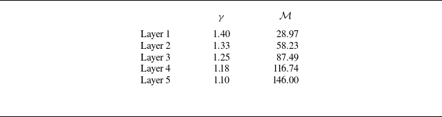To intuitively explore the effect of the diffusion layer on the refraction process, it is assumed that there are four gas interfaces ( $m_1, m_2, m_3, m_4$ ) within the diffusion layer, as shown in figure 11(b). These four interfaces represent a gradual transition of physical properties from one gas to another, and can effectively demonstrate the possibilities of wave formation within the diffusion layer. This assumption is made to simplify the problem and to allow for a step-by-step analysis of the refraction process within the diffusion layer. In fact, at least two gas interfaces are required, and more gas interfaces could more accurately reflect the physical state of the waves (such as pressure and flow deflection angles) in the diffusion layer. Although this assumption is not fully rigorous, it is a common approach in numerical and theoretical studies to discretise continuous regions into manageable elements for analysis. On both sides of each interface, there are uniform gas layers with specific heat ratios and molecular weight ratios as listed in table 1. In the following, the interactions between an incident shock with $\xi _i=0.66$ and four interfaces with $\omega _0$ of 60 $^\circ$ and 30 $^\circ$ , respectively, will be discussed, and the formation mechanism of RRR-E will be explored.

Table 1.

Parameters of specific heat ratio $\gamma$ and molecular weight $\mathcal {M}$ for different diffusion layers.

Figures 13(a) and 13(b) illustrate the refraction of the incident shock within the diffusion layer under the conditions $\xi _i=0.66$ and $\omega _{\textrm {0}}=\, 60$ $^\circ$ . When the incident shock interacts with the interface $m_1$ , the flow deflection angle behind the incident shock $\delta _{00}$ can be determined. However, at this deflection angle, the polar envelope of the transmitted shock is outside the polar envelope of the incident shock, indicating that the pressure behind the incident shock is higher than that behind the transmitted shock. Therefore, a reflected expansion wave is required to match the pressure relationship. The expansion wave polar $r_1$ is originated from a point on the incident shock polar, intersecting with the transmitted shock polar at the point $RE_1$ . When the transmitted shock $t_1$ generated from the interface $m_1$ becomes the incident shock and impinges the interface $m_2$ , the flow deflection angle $\delta _{01}$ can be determined. At this point, the polar envelope of the transmitted shock $t_2$ is inside the polar envelope of $t_1$ , indicating that the pressure behind the incident shock ( $t_1$ ) is less than that behind the transmitted shock ( $t_2$ ). Therefore, a reflected shock is needed to match the pressure relationship. The reflected shock polar $r_2$ is produced from point $RE_1$ on the polar $t_1$ , intersecting with the polar $t_2$ at point $RS_2$ . The interactions between the transmitted shock and subsequent interfaces only produce shocks, which gradually superimpose to form a stronger shock. The appearance of the expansion wave polar $r_1$ creates an interesting structure where the reflected waves include both an expansion wave and a shock. As a result, the present work theoretically verifies that both expansion wave and shock wave can be generated simultaneously when a shock refracts at a ‘fast–slow’ interface.

However, if $\omega _0$ changes to 30 $^\circ$ , as shown in figures 13(c) and 13(d), then when the incident shock interacts with the interface $m_1$ , the transmitted shock polar intersects with the reflected shock polar at point $RS_1$ . From this point on, all interactions between the transmitted shock and the interfaces will reflect shocks. These shocks gradually superimpose to form a stronger reflected shock. There is no expansion wave between the incident and reflected shocks.

Figure 13.

Polar diagrams showing the refraction of a planar shock with $\xi _i=\, 0.66$ at the diffusive air-SF $_6$ layer, for (a,b) $\omega _{\textrm {0}}=\, 60$ $^\circ$ and (c,d) $\omega _{\textrm {0}}=\, 30$ $^\circ$ . Here, $RE$ ( $RS$ ) is the intersection of the reflected expansion wave polar (reflected shock polar) with the transmitted shock polar; and $\delta _{00}$ and $\delta _{01}$ are the flow deflection angles caused by the incident shock and the expansion wave, respectively.

4.2. Theoretical analysis of refraction modes in the diffusion layer

From the analysis in § 4.1, it can be concluded that the generation of an expansion wave is represented in the shock polar diagram as the intersection of the transmitted shock polar and the reflected expansion wave polar. However, it is not rigorous to assume the diffusion layer as a finite number of thin parallel inviscid gas layers, as it is difficult to accurately find the conditions that exactly produce an expansion wave. To predict the conditions of RRR-E formation, it is necessary to seek answers on the shock polar diagrams. As shown in figure 12(a), there is a double solution $D_{\textrm {1}}$ between the transmitted shock polar and the incident shock polar, and there will also be two single solutions $A_{\textrm {1}}$ and $A_{\textrm {2}}$ under certain conditions, as shown in figure 12(b). The reflected shock or expansion wave polar has a double solution $D_{\textrm {2}}$ with the incident shock polar. An expansion wave can be generated only when $A_{\textrm {1}}$ and $A_{\textrm {2}}$ have no solutions, as shown in figure 12(a), or the ordinate values of $A_{\textrm {1}}$ and $A_{\textrm {2}}$ are less than that of $D_{\textrm {2}}$ , as shown in figure 13(b). In fact, the case of $A_{\textrm {1}}$ and $A_{\textrm {2}}$ having no solutions is actually a special case where the ordinate values of $A_{\textrm {1}}$ and $A_{\textrm {2}}$ approach that of $D_{\textrm {1}}$ infinitely. It is more general to analyse the case where the ordinate values of $A_{\textrm {1}}$ and $A_{\textrm {2}}$ are less than that of $D_{\textrm {2}}$ . Since the ordinate values of $A_{\textrm {1}}$ and $A_{\textrm {2}}$ are the same, and only $A_{\textrm {1}}$ has physical significance in the present analysis, $A_{\textrm {2}}$ will not be discussed in subsequent analyses.

The ordinate value of $A_{\textrm {1}}$ ( $\epsilon =p_{\textrm {1},T_i}/p_{\textrm {0},B_i}$ ) can be obtained by solving (4.1):

(4.8) \begin{equation} \begin{aligned} \displaystyle \tan \delta _{\textrm {0},B_i}= \frac {\epsilon -1}{1+\gamma _{\textrm {0},B_i} M_{\textrm {0},B_i}^2 -\epsilon } \times \left (\frac {\displaystyle \frac {2\gamma _{\textrm {0},B_i}}{\gamma _{\textrm {0},B_i}+1} M_{\textrm {0},B_i}^2-\displaystyle \frac {\gamma _{\textrm {0},B_i}-1}{\gamma _{\textrm {0},B_i}+1}-\epsilon }{\displaystyle \frac {\gamma _{\textrm {0},B_i}-1}{\gamma _{\textrm {0},B_i}+1}+\epsilon }\right ) ^{{1}/{2}}. \end{aligned} \end{equation}

It is worth noting that when the incident shock interacts with the diffusion interface, the physical properties of the gas within the diffusion layer must be distributed in some manner, which inevitably affects the propagation of the shock. However, in the present analysis, it is simply assumed that the velocity within the layer varies monotonically, without specifying a particular distribution form (such as Gaussian or exponential). Therefore, it is impossible to accurately determine the variation of the pressure ratio within the diffusion layer. Actually, the pressure ratio $\epsilon$ in (4.8) only corresponds to the conditions required for the formation of the RRR-E pattern near the air side (ambient gas). As a result, the pressure ratio in the diffusion layer may only affect the transmitted shock behaviour, but does not affect the formation conditions of the RRR-E pattern. For the convenience of mathematical operations, the relevant variables in the above equation are substituted:

(4.9) \begin{equation} \begin{aligned} \displaystyle &\delta _{\textrm {0}}=\delta _{{B}_i},\quad p_{\textrm {1}}/p_{\textrm {0}}=p_{{T_i}}/p_{{B_i}},\\ &a_1=1+\gamma _{\textrm {0}} M_{\textrm {0}}^2,\quad a_2=1+\mu \gamma _{\textrm {0}} M_{\textrm {0}}^2,\\ &b_1=\displaystyle \frac {2\gamma _{\textrm {0}} M_{\textrm {0}}^2}{\gamma _{\textrm {0}}+1}-\displaystyle \frac {\gamma _{\textrm {0}}-1}{\gamma _{\textrm {0}}+1},\quad b_2=\displaystyle \frac {2\mu \gamma _{\textrm {0}} M_{\textrm {0}}^2}{\gamma _{{B_i}}+1}-\displaystyle \frac {\gamma _{{B_i}}-1}{\gamma _{{B_i}}+1},\\ &c_1=\displaystyle \frac {\gamma _{\textrm {0}}-1}{\gamma _{\textrm {0}}+1},\quad c_2=\displaystyle \frac {\gamma _{{B_i}}-1}{\gamma _{{B_i}}+1}, \end{aligned} \end{equation}

where $\mu = {\mathcal {M} _{{B_i}}}/{\mathcal {M} _0}$ . Then from (4.8) and (4.9), it can be derived that

(4.10) \begin{equation} \begin{aligned} \displaystyle \frac {{(a_2-\epsilon )}^2}{{(a_1-\epsilon )}^2} = \frac {(b_2-\epsilon )}{(c_2+\epsilon )} \frac {(b_1-\epsilon )}{(c_1+\epsilon )}. \end{aligned} \end{equation}

In previous work (Henderson Reference Henderson1967b ), only the variation in flow Mach number was involved, but the effect of the specific heat ratio was ignored, resulting in a single algebraic equation of degree 2. However, in the present discussion, the effects of both the specific heat ratio and the molecular weight ratio of the gases are considered simultaneously, hence resulting in a single polynomial equation of degree 3 with $\epsilon = p_{{T_i}}/p_{{B_i}}$ as the variable:

(4.11) \begin{equation} \begin{aligned} \displaystyle \chi _1 \epsilon ^3 + \chi _2 \epsilon ^2 + \chi _3 \epsilon + \chi _4 = 0, \end{aligned} \end{equation}

where $\chi _1$ , $\chi _2$ , $\chi _3$ and $\chi _4$ are the coefficients, which can be expressed as

(4.12) \begin{equation} \begin{aligned} \displaystyle & \chi _1 = -2 a_1 + 2 a_2 + b_1 - b_2 + c_1 - c_2,\\ & \chi _2 = a_1^2 - a_2^2 - 2 a_2 b_1 + 2 a_1 b_2 - 2 a_1 c_1 - b_2 c_1 + 2 a_2 c_2 + b_1 c_2,\\ & \chi _3 = a_2^2 b_1 - a_1^2 b_2 + a_1^2 c_1 - a_2^2 c_2 + 2 a_1 b_2 c_1 - 2 a_2 b_1 c_2,\\ & \chi _4 = - a_1^2 b_2 c_1 + a_2^2 b_1 c_2. \end{aligned} \end{equation}

Figure 14.

The distribution of parameter space for single solution $A_1$ and double solution $D_2$ at $\xi _i=\, 0.66$ and $\omega _0=\, 60$ $^\circ$ . The blue surface represents the distribution of the double solution $D_2$ , and the red surface represents the distribution of the single solution $A_1$ . The white dashed line represents the distribution of Mach lines.

Although there is a general solution for the polynomial equation of degree 3, its expression is too complex, and a computer program is utilised to solve (4.11). From the expressions of (4.12), the variation of $\epsilon$ is controlled by the ratio of specific heats $\gamma _{{B_i}}$ and the molecular weight ratio $\mu$ of the gas layers. Therefore, solutions are sought in the parameter space where the specific heat ratio $\gamma _{{B_i}}$ ranges from 1.1 to 1.9, and the molecular weight ratio $\mu$ varies between 1.05 and 3 (the solutions will diverge when $\mu$ is too small). The computational results are provided in figure 14. Note that during the calculation, when the imaginary part of the solution is less than $1\times 10^{-5}$ , it is considered as 0, thus the solution is regarded as a real root. In addition, the results shown in figure 14 are from one of the solutions to (4.12), while the other two solutions are discarded because they involve imaginary roots.

In figure 14, the red surface represents the parameter space in which the incident and transmitted shock polars in the diffusion layer intersect at the single solution point $A_1$ . The blue surface represents the intersection point $D_2$ of the incident shock polar with the reflected wave polar within the diffusion layer. The white dashed line indicates the limit situation where the reflected shock degenerates into a Mach line. It can be observed that on one side of the Mach line, the value of $A_1$ is greater than that of $D_2$ , and the pressure behind the incident shock is less than that behind the transmitted shock. To match the pressure difference, a reflected shock wave is generated from the interface. On the other side, the value of $A_1$ is less than that of $D_2$ , and therefore an expansion wave is reflected, forming RRR-E. Moreover, the physical properties in the diffusion layer should transition continuously from air to SF $_6$ . On the side close to air, the acoustic impedance of the gas in the diffusion layer is similar to air, making it possible for an expansion wave to form at the interface, as shown in figure 13. As one moves closer to SF $_6$ within the diffusion layer, the properties of the gas become more like those of SF $_6$ , making it easier to produce a shock wave at the interface. Therefore, RRR-E can form only when the specific heat ratio $\gamma$ is close to 1.4, and the value of $A_1$ is less than that of $D_2$ . Here, we should emphasise that the RRR-E pattern in the present work forms only when the specific heat ratio $\gamma$ is close to 1.4, because the ambient gas is air with specific heat ratio 1.4. If the ambient gas is helium with specific heat ratio 1.66, then the RRR-E pattern would form when $\gamma$ is close to 1.66. As a result, the RRR-E pattern is not a fairly rare phenomenon. Due to the divergence of solutions at $\mu =\, 1$ and $\gamma =\, 1.4$ , the numerical magnitudes of $A_1$ and $D_2$ are assessed at $\mu =\, 1.02$ and $\gamma =\, 1.4$ to determine whether RRR-E will form or not.

Figure 15.

The phase diagram showing the refraction patterns. All the solid lines are derived from Abd-El-Fattah & Henderson (Reference Abd-El-Fattah and Henderson1978a ), representing the boundaries between refraction patterns at a sharp interface. The different regions enclosed by these solid lines are indicated by different colours, representing the various refraction patterns at the sharp interface obtained theoretically. All the circular symbols come from the present numerical results. The triangles represent the results calculated using (4.11). The red dashed line is the fitted boundary between RRR and RRR-E calculated by (4.13).

To verify the accuracy of the aforementioned model, the phase diagram showing the refraction patterns at an air–SF $_6$ interface is plotted in figure 15. The red triangles calculated by (4.11) represent the critical solutions of the RRR $\rightarrow$ RRR-E transition. Because the method through figure 14 requires us to judge whether there is a possibility of generating RRR-E or not under certain initial conditions, the red triangles in figure 15 are all discrete points. In order to compare with the phase diagram of the sharp interface, the discrete computational results are fitted to obtain the equation

(4.13) \begin{equation} \begin{aligned} \displaystyle \xi _i = 1.72 \times 10 ^{-3} \omega _0^2 - 0.24 {\omega _0} + 8.13. \end{aligned} \end{equation}

All circular symbols in figure 15 represent the numerical results at $C_i = 10$ . The purple and brown circular symbols represent RRR and RRR-E, respectively. Both these symbols are well distributed on either side of the transition line described by (4.13), which demonstrates that the present model can reasonably predict the conditions for the emergence of RRR-E. All the solid lines are derived from Abd-El-Fattah & Henderson (Reference Abd-El-Fattah and Henderson1978a ), representing the boundaries between refraction patterns at a sharp interface. The different regions enclosed by these solid lines are indicated by different colour blocks, representing the various refraction patterns at the sharp interface obtained theoretically. The orange and blue solid lines are obtained based on the condition $M_1=\, 1$ . In the previous work (Abd-El-Fattah & Henderson Reference Abd-El-Fattah and Henderson1978a ), the authors considered all refraction patterns to the right of $M_1=\, 1$ as CFR. In fact, a distinction should be made at one $\xi _i^\ast$ , as shown in figure 15, where for $ \xi _i \gt \xi _i^\ast$ , the refraction pattern to the right of $M_1=\, 1$ should be ARE, and when $ \xi _i \lt \xi _i^\ast$ , it should be CFR. For the air–SF $_6$ interface, the value of $\xi _i^\ast$ is approximately 0.73.

At a sharp interface, it is commonly accepted that MRR will occur in the region between $ \alpha _1 = A_1 =\beta _1$ and $ \alpha _1 = \alpha _2$ , and the region between $ \alpha _1 = \alpha _2$ and $M_1=\, 1$ . However, at the diffusion interface, the transition line described by (4.13) crosses through the later region, and MRR even occurs in the region to the right of $M_1=\, 1$ . This indicates that the appearance of MRR is delayed due to the emergence of RRR-E. This is of significant value for the structural design of the combustion chamber in scramjet engines. When considering the interaction between shock waves and fuel, the fuel interface cannot be simply regarded as an infinitely thin layer, and the diffusion effect should be considered. Overall, the shock refraction at the diffusive interface is accompanied by the emergence of new phenomena, and the existing transition laws for sharp interfaces are no longer accurate.