1 Introduction
Physiological flows through arterial vessels are complex due to unsteady or pulsatile and spatially developing conditions. Curvature, which can be high in the ascending aorta for example, brings in additional complexity due to secondary flows which are caused by an imbalance between centrifugal forces and the radial pressure gradients. Unsteady flows in curved pipes are also important in several engineering applications such as heat exchanger tubes and in internal combustion engines (Kalpakli et al.
Reference Kalpakli, Örlü, Tillmark and Alfredsson2011). A variety of flows in curved tubes have been studied using analytic, experimental and numerical methods (McConalogue & Srivastava Reference McConalogue and Srivastava1968; Lyne Reference Lyne1971; Singh Reference Singh1974; Chandran & Yearwood Reference Chandran and Yearwood1981; Talbot & Gong Reference Talbot and Gong1983; Sudo, Sumida & Yamane Reference Sudo, Sumida and Yamane1992; Komai & Tanishita Reference Komai and Tanishita1997; Siggers & Waters Reference Siggers and Waters2008). Broadly, most flows are classified as steady or unsteady, and fully developed or spatially developing. Flows where the conditions do not change spatially in the flow direction are said to be fully developed. The flow rate may, however, change over time, and is accompanied by pressure gradients changing direction; these often lead to reversals of flow. Curvature introduces secondary flows in the transverse cross-section. The interactions between the unsteadiness and curvature components can be highly nonlinear and result in a rich variety of flow structures which have been observed in unsteady flows through curved pipes. Three types of unsteady flow in curved pipes with uniform cross-section have been reported based on changes in the volume flow rate with time: first, oscillatory flows, where the flow rate averaged over the time pulse is zero (Mullin & Greated Reference Mullin and Greated1980a
; Chang & Tarbell Reference Chang and Tarbell1985; Sudo et al.
Reference Sudo, Sumida and Yamane1992); second, pulsatile flows, where an oscillatory flow is superimposed on a steady component (Talbot & Gong Reference Talbot and Gong1983; Chang & Tarbell Reference Chang and Tarbell1985; Hamakiotes & Berger Reference Hamakiotes and Berger1988; Komai & Tanishita Reference Komai and Tanishita1997; Timité, Castelain & Peerhossaini Reference Timité, Castelain and Peerhossaini2010); finally, single pulse, where the flow is present over a short time period with zero net flow condition before and after the pulse (Komai & Tanishita Reference Komai and Tanishita1997; Boiron, Deplano & Pelissier Reference Boiron, Deplano and Pelissier2007). The parameters that are used to characterize unsteady flows in a curved tube are the Reynolds number
 $(Re)$
, those related to curvature effects, which include the curvature ratio
 $\unicode[STIX]{x1D6FD}$
(
 $=a/R$
), where
 $a$
is the tube radius and
 $R$
is the radius of curvature, and the Dean number
 $(De)$
, and the Womersley number
 $(\unicode[STIX]{x1D6FC})$
, which arises due to flow unsteadiness. The Dean number is defined as
 $De=Re\sqrt{\unicode[STIX]{x1D6FD}}$
, where
 $Re$
is the Reynolds number based on the axial flow velocity. The Dean number hence represents the relative importance of the product of inertia and centrifugal forces to the viscous forces. There are many definitions of
 $De$
in the literature (Berger, Talbot & Yao Reference Berger, Talbot and Yao1983); for consistency, we define, unless otherwise stated,
 $De$
based on the maximum area averaged axial flow velocity for all cited references in our study. For flow rates that vary periodically with time, the Womersley number is given in terms of the angular frequency,
 $\unicode[STIX]{x1D714}$
, as
 $\unicode[STIX]{x1D6FC}=a\sqrt{\unicode[STIX]{x1D714}/\unicode[STIX]{x1D708}}$
. The Womersley number can be thought of as the ratio of
 $a$
to the diffusive or Stokes layer thickness,
 $\unicode[STIX]{x1D6FF}\sim \sqrt{\unicode[STIX]{x1D708}/\unicode[STIX]{x1D714}}$
, where
 $\unicode[STIX]{x1D708}$
is the kinematic viscosity.
Early pioneering work by Dean (Reference Dean1927, Reference Dean1928) for steady, laminar and fully developed flows with low values of
 $\unicode[STIX]{x1D6FD}$
showed analytically the presence of two symmetric counter-rotating vortices in the transverse cross-section. Dean’s analysis is valid for loosely curved pipes
 $(\unicode[STIX]{x1D6FD}\ll 1)$
, which indicate low curvature, and for Dean number based on pressure gradient
 ${<}\,96$
. Other studies have extended this analysis to higher
 $De$
values using analytical and numerical methods (McConalogue & Srivastava Reference McConalogue and Srivastava1968; Collins & Dennis Reference Collins and Dennis1975; Dennis & Ng Reference Dennis and Ng1982; Berger et al.
Reference Berger, Talbot and Yao1983). With increase in
 $De$
, the secondary flow strength increases and the axial velocity peak shifts towards the outer wall. At high values of
 $De$
, a boundary layer develops, with the viscous layers confined near the tube walls and an outer inviscid flow that is retained in the core. Boundary layer techniques have been used to analyse such flows (e.g. Barua Reference Barua1963; Mori & Nakayama Reference Mori and Nakayama1965; Itō Reference Itō1969). The
 $De$
appears as a single non-dimensional parameter for steady flows only for loosely curved tubes; for highly curved tubes, the
 $\unicode[STIX]{x1D6FD}$
values are not small and both
 $De$
or
 $Re$
and
 $\unicode[STIX]{x1D6FD}$
are present as independent non-dimensional parameters. Steady entry flow in a curved tube is an important not fully developed flow situation which has been investigated in several studies (Singh Reference Singh1974; Agrawal, Talbot & Gong Reference Agrawal, Talbot and Gong1978; Choi, Talbot & Cornet Reference Choi, Talbot and Cornet1979; Stewartson, Cebeci & Chang Reference Stewartson, Cebeci and Chang1980; Timité et al.
Reference Timité, Castelain and Peerhossaini2010) and has some features that are common to the unsteady flows in our study. For the case of uniform flow at the inlet and at high
 $Re$
, the flow is split into an inviscid core, where the radial pressure gradient balances the centrifugal force, and a viscous boundary layer that develops in the flow direction on the wall. This radial pressure gradient is imposed on the boundary layer, which drives the fluid from the outer to the inner wall. The fluid in the core region hence moves radially outwards; the resulting flow is thus helical, with opposite signs of helicity in the top and bottom halves of the tube. Singh (Reference Singh1974) used the method of matched asymptotic expansion and derived an analytical solution for the development of secondary flow in the entrance region, which is clearly different compared with a fully developed curved pipe flow. Most of the studies in curved pipes with square and rectangular cross-sections have looked at steady flows. Depending on the flow parameters, different solutions have been observed: two vortex, four vortex and more than four vortex systems. Analytical (Winters Reference Winters1987), numerical and experimental methods have been used to analyse these flows (Bara, Nandakumar & Masliyah Reference Bara, Nandakumar and Masliyah1992; Mees, Nandakumar & Masliyah Reference Mees, Nandakumar and Masliyah1996). Earlier studies were extended to higher Dean numbers and curvatures (Mondal et al.
Reference Mondal, Kaga, Hyakutake and Yanase2007; Machane Reference Machane2010). Mondal et al. (Reference Mondal, Kaga, Hyakutake and Yanase2007) gave a map indicating the nature of solution over a range of Dean number and curvature ratios; these are, however, for steady flows alone.
Much of the analytical work in fully developed oscillatory and pulsatile flows (i.e. for zero and non-zero mean flows) through curved tubes has been for loosely coiled tubes (
 $\unicode[STIX]{x1D6FD}\ll 1$
). The secondary streaming Reynolds number, defined as
 $R_{s}=\overline{W}^{2}a/(R\unicode[STIX]{x1D714}\unicode[STIX]{x1D708})$
, characterizes the secondary flow amplitude for fully developed oscillatory flow in a curved pipe; here,
 $\overline{W}$
is the axial velocity amplitude. Analytical solutions have been obtained in the limit of small and large
 $R_{s}$
and confirmed experimentally by Lyne (Reference Lyne1971). These studies showed that the secondary structures consist of two pairs of vortices. Further, the vortex in the inviscid core has a sense opposite to that in the steady flow. Several studies have since built on Lyne’s work (Zalosh & Nelson Reference Zalosh and Nelson1973; Mullin & Greated Reference Mullin and Greated1980b
). The secondary flow velocity scale was obtained from scaling arguments in loosely curved pipes for fully developed steady flows (Dennis & Riley Reference Dennis and Riley1991) and fully developed oscillatory flows (Waters & Pedley Reference Waters and Pedley1999). Through addition of a mean flow component, Smith (Reference Smith1975) showed analytically that the secondary flows are similar to the steady Dean flows for low values of
 $\unicode[STIX]{x1D6FC}$
. In contrast, the secondary flow field was altered for larger values of
 $\unicode[STIX]{x1D6FC}$
. Some of these results were confirmed experimentally by Bertelsen (Reference Bertelsen1975) and Munson (Reference Munson1975). Studies for fully developed or developing unsteady flows with finite curvature have mainly used numerical or experimental approaches, barring a few (e.g. Singh, Sinha & Aggarwal Reference Singh, Sinha and Aggarwal1978; Siggers & Waters Reference Siggers and Waters2005, Reference Siggers and Waters2008). One type of investigation has been to study and classify the many different secondary flow structures that occur due to pulsatile flows in
 $90^{\circ }$
(Timité et al.
Reference Timité, Castelain and Peerhossaini2010; Jarrahi, Castelain & Peerhossaini Reference Jarrahi, Castelain and Peerhossaini2011) or
 $180^{\circ }$
(Sudo et al.
Reference Sudo, Sumida and Yamane1992; Glenn et al.
Reference Glenn, Bulusu, Shu and Plesniak2012; Bulusu & Plesniak Reference Bulusu and Plesniak2013) curved tubes. The nature and structure of these secondary flow structures depend on
 $Re$
,
 $\unicode[STIX]{x1D6FC}$
and the ratio of the mean to pulsatile components of velocity. A different, but related, flow is a rotating fluid-filled torus which undergoes an impulsive change in its rotation speed (Del Pino et al.
Reference Del Pino, Hewitt, Clarke, Mullin and Denier2008; Hewitt et al.
Reference Hewitt, Hazel, Clarke and Denier2011). The fluid, initially in solid-body rotation, develops a boundary layer at the wall under these conditions, which develops a secondary flow due to a radial pressure gradient in the inviscid core. The boundary layers from the top and bottom halves collide in the medial plane, and the boundary layer fluid erupts into the core. The secondary flow structures and subsequent collision in the medial plane are much like those found in unsteady flows in curved pipes. Analytical solutions for developing or fully developed flows were obtained in curved pipes of circular cross-section (Stewartson et al.
Reference Stewartson, Cebeci and Chang1980; Riley Reference Riley1998). A singularity was shown in the solutions of boundary layer equations in the medial plane at the inner wall of the pipe after a finite streamwise distance (Stewartson et al.
Reference Stewartson, Cebeci and Chang1980) for steady developing flows, and following a finite time (Riley Reference Riley1998) for the case of fully developed unsteady flows; the boundary layer fluid subsequently erupts into the core.
We now discuss some studies that are directly relevant to our present work on unsteady developing flows in a curved tube with finite curvature. Chandran & Yearwood (Reference Chandran and Yearwood1981) reported velocity profiles using a three-dimensional hot-film anemometer placed at different locations along the bend for a physiological input velocity profile using a pulse duration of 1 s, with a systolic duration of 370 ms (
 $\unicode[STIX]{x1D6FC}=20.76$
), for a tube with curvature ratio
 $\unicode[STIX]{x1D6FD}=0.1$
. The
 $Re$
and
 $De$
, calculated using the peak velocity, were 3300 and 1140 respectively. Based on experimentally obtained velocity profiles, they showed the presence of a strong reverse flow region near the inner wall at the beginning of diastole, and movement of the peak axial velocity location across the transverse section of the tube during the cycle. In continuation of this study, Yearwood & Chandran (Reference Yearwood and Chandran1982) investigated physiological flows in a pipe with a higher curvature (
 $\unicode[STIX]{x1D6FD}\sim 0.4$
), created using phantoms of ascending aorta, and again found significant reverse flows along the inner wall during the deceleration phase. Since these seminal works, there have been several experimental and numerical studies (Chang & Tarbell Reference Chang and Tarbell1985; Konno, Satoh & Tanishita Reference Konno, Satoh and Tanishita1994; Komai & Tanishita Reference Komai and Tanishita1997) in tubes of high curvature that essentially report similar findings. Komai & Tanishita (Reference Komai and Tanishita1997) explored the effects of pulsatility on fully developed flows in curved tubes, by varying the time between pulses, to investigate the effects of the residual secondary structures on the following cycle. They also explored, as an extreme case, the resulting flow structures due to a single pulse. The Dean number was fixed at 786,
 $1/7\leqslant \unicode[STIX]{x1D6FD}\leqslant 1/2$
,
 $1112\leqslant Re\leqslant 2080$
and
 $4\leqslant \unicode[STIX]{x1D6FC}\leqslant 27$
. In addition to the observation of flow reversal during deceleration near the inner wall, they clearly showed the existence of a secondary flow near the walls and an outward radial jet in the transverse plane from the inner wall towards the outer one. More recently, Boiron et al. (Reference Boiron, Deplano and Pelissier2007) used experiments and numerical computations to study the flow in a
 $180^{\circ }$
curved pipe of circular cross-section with relatively low curvature (
 $\unicode[STIX]{x1D6FD}=0.07$
) using a physiological input flow profile. They reported similar flow features to those in earlier studies, namely collision of secondary structures in the medial plane and a subsequent radial outward jet, and provided some insight into the jet motion by exploring the individual contributions from various terms in the governing momentum equation in the radial direction of the medial plane. A large variety of structures have been observed; few studies have explored the origin of these secondary flow structures. Further, none of these studies give scales for the secondary velocity for unsteady flow in highly curved pipes, which can be used to quantify the various flow parameters like movement of vortical structures and wall shear stress.
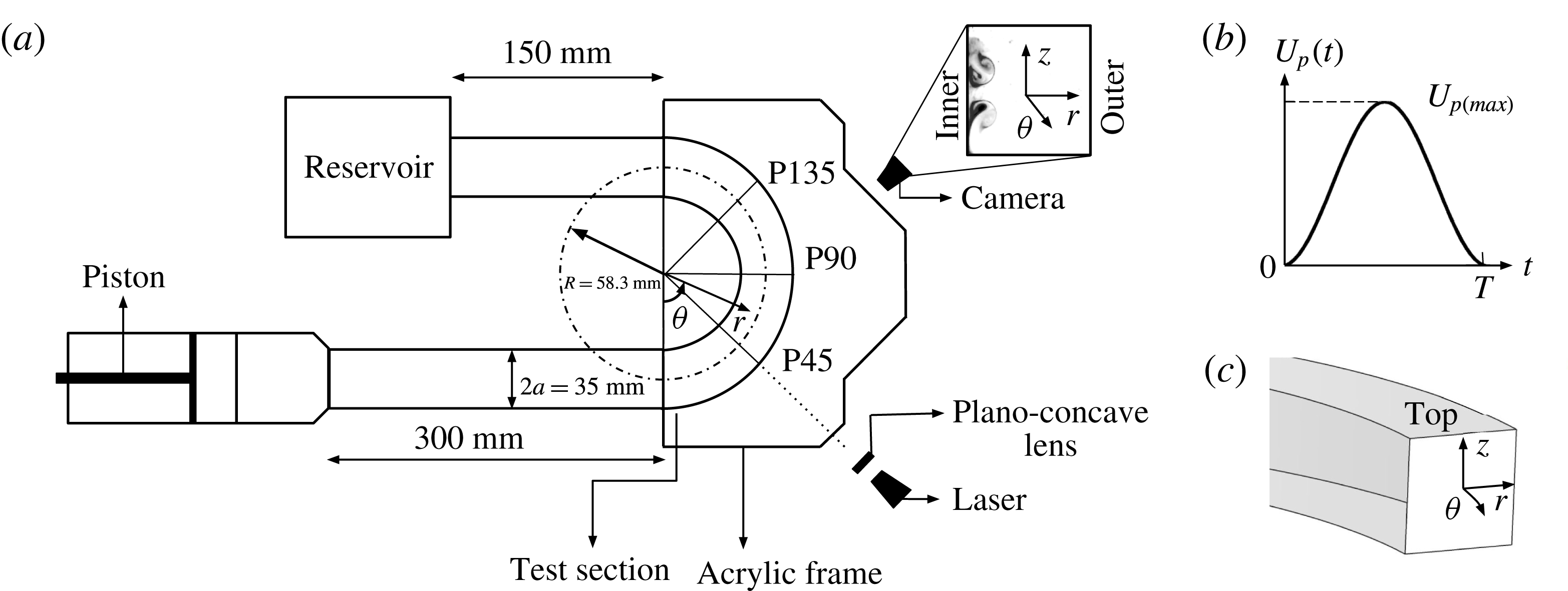
(a) A servo motor was connected to a piston and used to drive the fluid to obtain different flow velocities. The test section was a custom-built acrylic square tube which was immersed in an acrylic water-filled frame to reduce optical lensing. The outlet of the test section was connected to a reservoir. Fluorescein dye along with a solid-state laser was used in flow visualization studies, performed in three transverse (
 $r{-}z$
) planes, indicated as P45, P90 and P135, and a horizontal (
 $r{-}\unicode[STIX]{x1D703}$
) plane. (b) Variation in the input piston velocity,
 $U_{p}(t)$
, is shown with time,
 $t$
. The pulse width of the cycle is
 $T$
. (c) A cross-sectional view of the acrylic section is shown and the coordinate system is indicated.

In this study, we used a
 $180^{\circ }$
acrylic highly curved pipe
 $(\unicode[STIX]{x1D6FD}=0.3)$
with a square cross-section, and investigated the presence of various flow structures over a wide range of
 $De{-}\unicode[STIX]{x1D6FC}$
. The unsteady flow is in the form of a single pulse whose duration and amplitude are varied. Our study is especially relevant to physiological blood flows in the ascending aorta, which consist of a systolic period, when the flow rate is non-zero, which is followed by diastolic period when the flow rate is essentially zero. We also used numerical methods to obtain quantitative information to better understand the complex flow dynamics in highly curved pipes. We observe the development of secondary flow, collision of vortical structures in the medial plane and their subsequent movement into the core. Our results show that both curvature, through
 $De$
, and unsteadiness, through
 $\unicode[STIX]{x1D6FC}$
, when varied independently and in consonance, introduce large changes in the flow structures. We characterized variations in the wall shear stress (WSS) that depend on the combined effects of pulsatility and strength of secondary flow structures in the curved tube. Finally, we used scaling analysis to estimate the strength of the secondary structures. We believe that our studies will be helpful in understanding the flow physics for a wider class of curved tube flows which are also relevant in many engineering applications.
2 Methods
2.1 Experimental set-up
The custom-made experimental flow loop (figure 1
a) consisted of a
 $180^{\circ }$
acrylic curved pipe and a piston pump (bore diameter 10 cm and stroke length 20 cm) driven by a servo motor and controlled using a driver (MCDDT3520; Panasonic). The control signal to the driver unit was generated by a data acquisition card (National Instruments CDAQ-9172) using a virtual instrument in LabView 7.1 (National Instruments, Austin, Texas). The piston was connected to a curved tube test section which was fabricated with a square cross-section (radius of curvature from centreline
 $R=60.3\pm 1.5$
mm; edge length
 $2a=34.8\pm 0.5$
mm). A square cross-section allowed us to visualize the flow structures clearly without any refraction effects. The straight walls permitted us to clearly establish the origin of secondary flows, as we shall show later. The inlet length of the test section was approximately 8.5 edge lengths from the piston to the beginning of the curved section to permit fully developed flow at the entrance of the curved section. This length was selected to ensure that the disturbances from the inlet did not convect into the test section. The outlet, fabricated to be approximately 4.2 edge lengths from the end of the curved region, was connected to a reservoir tank. The experiments were conducted using deionized distilled water. Ports on each side of the four walls were bored at the beginning of the curved section and were used to inject fluorescein dye. The port located at the inner wall was used for visualization studies in the medial (
 $r{-}\unicode[STIX]{x1D703}$
) plane; the ports on the straight sides were used for visualization in the cross-sectional planes. For the port on the bottom wall, the dye was mixed with common salt to obtain a density of
 $1010~\text{kg}~\text{m}^{-3}$
such that the dye settled in the bottom regions of the tube at the start of the visualization studies. In contrast, the density was lowered to
 $990~\text{kg}~\text{m}^{-3}$
for visualization studies in the top half of the test section using ethyl alcohol. The density difference was sufficiently small so that the dye faithfully followed the flow and the buoyancy forces were negligible (Das & Arakeri Reference Das and Arakeri1998). An acrylic water-filled frame, with view planes cut at
 $45^{\circ }$
(P45),
 $90^{\circ }$
(P90) and
 $135^{\circ }$
(P135) from the inlet, was fitted around the test section to reduce the lensing effect. A 1 W continuous green laser with plano-concave lens was used to produce a light sheet in the flow visualization studies. The camera and laser positions were set in one of the three transverse (
 $r{-}z$
) planes, P45, P90, P135, or the horizontal plane for visualizing the flows. Four independent experiments were performed corresponding to each combination of
 $De$
and
 $\unicode[STIX]{x1D6FC}$
.
The variation of non-dimensional ‘piston’ velocity,
 $\hat{U} _{p}(t)$
, over time, normalized using the pulse width,
 $T$
, is given by (2.1) and shown in figure 1(b):
 $$\begin{eqnarray}\hat{U} _{p}(t)=\frac{U_{p}(t)}{U_{p(max)}}=\left\{\begin{array}{@{}ll@{}}(1-\cos (2\unicode[STIX]{x03C0}t/T))/2,\quad & \text{for}~t/T\leqslant 1,\\ 0,\quad & \text{otherwise}.\end{array}\right.\end{eqnarray}$$
Here,
 $U_{p}$
is the flow rate divided by the cross-sectional area of the pipe, or the area averaged axial velocity, and
 $U_{p(max)}$
is the peak area averaged axial velocity.
2.2 Numerical simulations
We performed numerical simulations using the ANSYS® FLUENT 13.0 (ANSYS Inc., Canonsburg, Pennsylvania) commercial solver for unsteady flows in a curved tube with the same geometry as that of the experimental test section, i.e. a straight inlet section, accompanied by a curved region of
 $180^{\circ }$
which ends in a straight outlet section. The inlet velocity variation with time used for the simulations was similar to those in the experimental set-up described earlier. We assumed Newtonian and incompressible fluid, and rigid walls in these simulations. The governing equations are given by the standard continuity and Navier–Stokes equations:
 $$\begin{eqnarray}\displaystyle & \unicode[STIX]{x1D735}\boldsymbol{\cdot }\boldsymbol{u}=0, & \displaystyle\end{eqnarray}$$
 $$\begin{eqnarray}\displaystyle & \displaystyle \frac{\unicode[STIX]{x2202}\boldsymbol{u}}{\unicode[STIX]{x2202}t}+\boldsymbol{u}\boldsymbol{\cdot }\unicode[STIX]{x1D735}\boldsymbol{u}=-\frac{1}{\unicode[STIX]{x1D70C}}\unicode[STIX]{x1D735}p+\unicode[STIX]{x1D708}\unicode[STIX]{x1D6FB}^{2}\boldsymbol{u}, & \displaystyle\end{eqnarray}$$
where
 $\boldsymbol{u}$
is the velocity,
 $p$
is the static pressure and
 $\unicode[STIX]{x1D70C}$
is the density. A no-slip boundary condition was applied on the wall. We used a constant-pressure boundary condition at the outlet, and specified a spatially uniform but time varying velocity at the inlet, given by (2.1). To satisfy the no-slip condition at the wall, the velocity at the boundary nodes was set to 0. We solved the governing equations with the boundary conditions using a finite-volume method based on a segregated solver. In this, we used the SIM-PLEC algorithm for pressure–velocity coupling. We integrated the transient terms using a second-order implicit formulation and a second-order upwind scheme for the convection terms. The diffusion terms were central differenced and are accurate to second order. The time step was advanced when the residuals for the continuity equation and each of the three velocity components were less than
 $10^{-5}$
. Finally, we used ANSYS® CFD Post 13.0 (ANSYS Inc., Canonsburg, Pennsylvania) and MATLAB® Release 2014a, (The MathWorks Inc., Natick, Massachusetts) for analysing and post-processing the results.
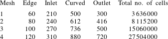
The number of cells used in each successive mesh refinement is indicated for the edge, inlet, curved region and outlet of the test section in the numerical simulations.

The geometry and mesh were created in ANSYS® ICEM 13.0 (ANSYS Inc., Canonsburg, Pennsylvania). A two-dimensional (2D) mesh, discretized with quadrilateral elements, was extruded along the centreline of the pipe to generate a three-dimensional (3D) volume mesh with hexahedral elements. A finer mesh was used to resolve the larger gradients in the boundary layers. Numerical simulations for a straight pipe with circular cross-section of the same diameter as that of the edge length of the square pipe were used to optimize the boundary layer mesh adjacent to the wall. The two parameters in a boundary layer mesh are the first length (the distance of the first cell from the wall) and the growth rate (ratio of distances between adjacent cells in the direction normal to the wall). The number of cells in the direction normal to the boundary layer was adjusted to ensure smooth transition from the boundary layer mesh to the core. Based on these simulations, we chose a first length of
 $1.44\times 10^{-5}$
m, a growth rate of 1.2 and 20 cells in the direction normal to the boundary layer; the change in the velocity gradients at the wall was less than 0.5 % and the root-mean-square error in the velocity was less than 0.1 % compared with the analytical solution given by Das & Arakeri (Reference Das and Arakeri1998) for the case with highest
 $Re\sim 10271$
and lowest
 $\hat{\unicode[STIX]{x1D6FF}}\sim 0.14$
. The ratio of the thickness of the boundary layer mesh to the half edge length was 0.15. These parameters were used for the boundary layer in the curved pipe with square cross-section in our study.
Table 1 shows the resolutions corresponding to different meshes that were tested to obtain grid-independent velocity profiles. The numbers of cells along each edge in the 2D mesh, including the ones in the boundary layer, are shown in table 1. Also shown are the numbers of cells in each of the sections (inlet, curved and outlet) along the centreline. The last column in table 1 shows the total number of cells for each mesh. Between the two meshes with the highest resolution (meshes 3 and 4), the changes in maximum velocity, minimum velocity and the root-mean-square difference in the velocity profile in both the axial and radial directions were less than 1 % throughout the time pulse, for all simulated cases except one (
 $Re\sim 3622$
,
 $\hat{\unicode[STIX]{x1D6FF}}\sim 0.41$
). For this case, the errors were slightly higher at the end of the cycle, where, as we shall see below, the flow becomes complicated. Mesh 3 was chosen for all of the simulations reported in this paper. The chosen time step in these simulations was
 $10^{-3}~\text{s}$
. For the 2D simulations, the mesh contained 144 cells along the edge, 396 in the inlet, 992 in the curved section and 817 in the outlet region. The total number of cells was 159 240 and the same boundary conditions, convergence criterion and discretization scheme were implemented as those for the full 3D simulations.
2.3 Non-dimensional parameters
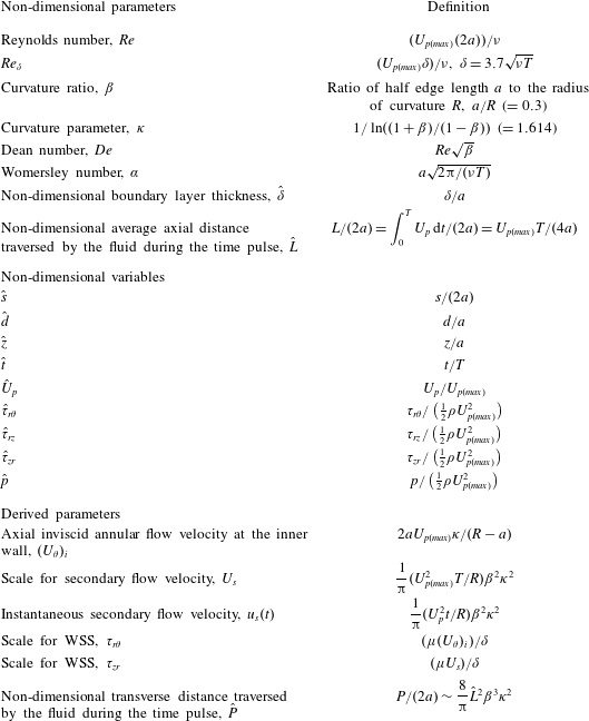
Table 2 lists the important parameters, which include the
 $Re$
,
 $De$
and
 $\unicode[STIX]{x1D6FC}$
. It should be noted that because the input velocity profile is neither oscillating nor pulsatile, the Womersley number, which is normally reported based on frequency, is calculated in our case using the duration of the pulse,
 $T$
, as
 $\unicode[STIX]{x1D6FC}=a\sqrt{2\unicode[STIX]{x03C0}/(\unicode[STIX]{x1D708}T)}$
. For flow in the ascending aorta, the time period essentially represents the systolic phase. In addition, we define other parameters, which can be written in terms of the above three, but which are useful when viewed independently to yield additional insights into the flow dynamics. The term
 $\unicode[STIX]{x1D6FF}/a\sim 1/\unicode[STIX]{x1D6FC}$
is the normalized boundary layer thickness, which directly indicates the extent to which viscous effects are important. Das (Reference Das1998) proposed a relation to calculate the boundary layer thickness for unsteady laminar fully developed flow created by a single pulse in a straight pipe over a range of input parameters (
 $250\leqslant Re_{\unicode[STIX]{x1D6FF}}\leqslant 3000$
,
 $0.1\leqslant \hat{\unicode[STIX]{x1D6FF}}\leqslant 0.91$
). The boundary layer thickness is given by
 $\unicode[STIX]{x1D6FF}=3.7\sqrt{\unicode[STIX]{x1D708}T}$
, which is the relation used in this study. The Reynolds number based on the boundary layer thickness (
 $Re_{\unicode[STIX]{x1D6FF}}=U_{p(max)}\unicode[STIX]{x1D6FF}/\unicode[STIX]{x1D708}$
) is a useful parameter to describe instability and transition of the inflection point velocity profiles (Das & Arakeri Reference Das and Arakeri1998; Das, Srinivasan & Arakeri Reference Das, Srinivasan and Arakeri2016). The term
 $\hat{L}=U_{p(max)}T/(4a)$
represents the average distance the fluid moves in the axial direction over the time period
 $T$
. Based on these quantities, we derive an expression for
 $\hat{P}$
, which represents the non-dimensional distance traversed by the secondary flows in the transverse (
 $r{-}z$
) plane. We will see that both
 $\hat{L}$
and
 $\hat{P}$
help in our understanding of the different structures observed as we vary
 $U_{p(max)}$
and
 $T$
. A parameter similar to
 $\hat{L}$
, called the formation length, has been used in vortex ring (Gharib, Rambod & Shariff Reference Gharib, Rambod and Shariff1998; Krueger & Gharib Reference Krueger and Gharib2003) and other unsteady flow studies (Das, Govardhan & Arakeri Reference Das, Govardhan and Arakeri2013a
). Table 2 also lists various scales for velocity and WSS which have been derived in later sections.
Nomenclature and definitions of various parameters used in the study.

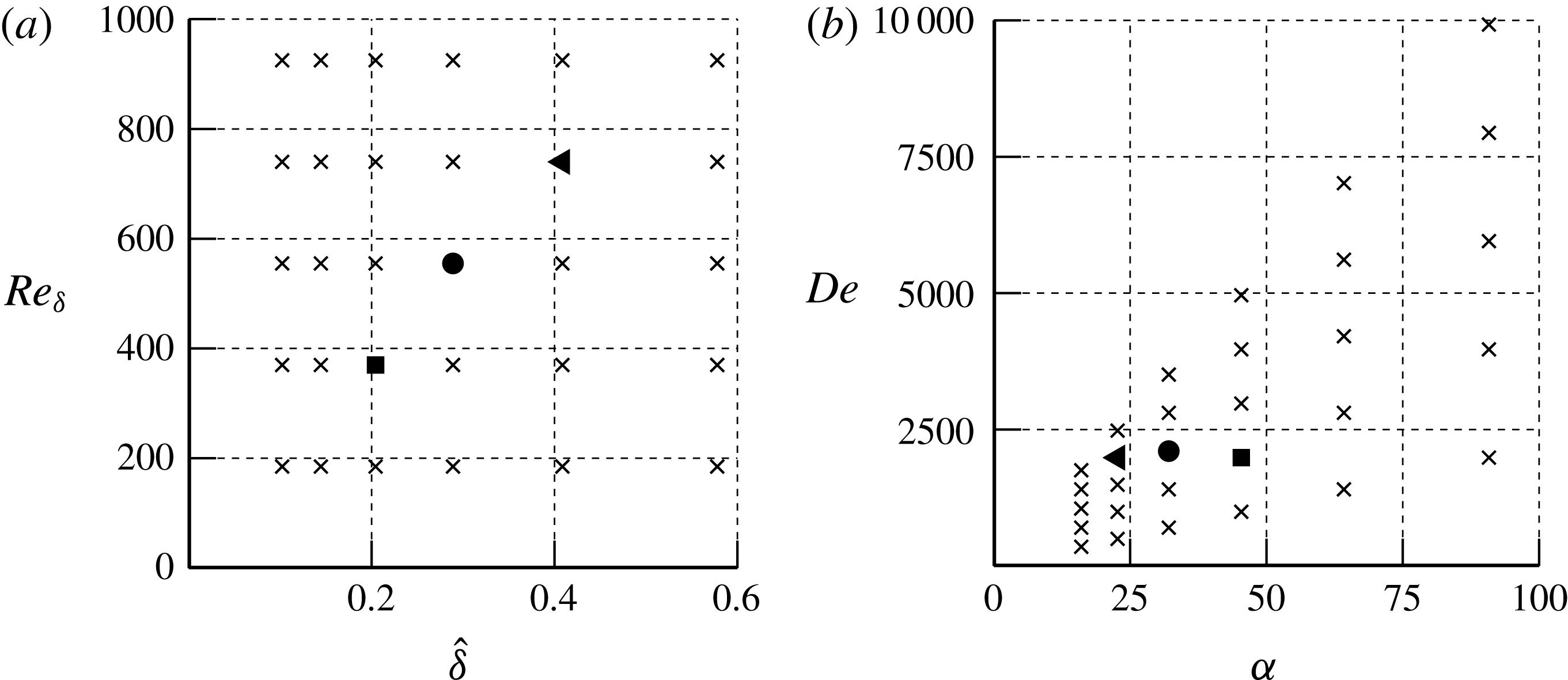
Figure 2(a) shows the range of
 $Re_{\unicode[STIX]{x1D6FF}}$
and
 $\hat{\unicode[STIX]{x1D6FF}}$
values, marked using the symbol (
 $\times$
) to indicate points where experiments were performed by varying the pulse duration and piston velocity. Figure 2(b) shows the values of
 $De$
and
 $\unicode[STIX]{x1D6FC}$
corresponding to these experiments. The ranges of values of the different variables are
 $0.0184\leqslant U_{p(max)}~(\text{m}~\text{s}^{-1})\leqslant 0.5199$
,
 $0.23\leqslant T~(\text{s})\leqslant 7.43$
,
 $640\leqslant Re\leqslant 18110$
and
 $0.3\leqslant \hat{L}\leqslant 9.8$
. Three cases were selected (table 3), which correspond to cases discussed in detail in § 3. Case 2 corresponds to a typical physiological case of flow in the ascending aorta (Lantz et al.
Reference Lantz, Renner, Länne and Karlsson2015). Two additional cases were investigated (cases 1 and 3), which have similar Dean numbers but different time periods. Case 1 corresponds to twice the time period of case 2; case 3 corresponds to half that of case 2. Numerical simulations were performed for five more cases in addition to the cases mentioned in table 3:
 $(De,\unicode[STIX]{x1D6FC})=(351,16)$
, (1400, 32), (1488, 23), (2976, 46) and (5625, 46). In all of the cases reported in the present work, we used the velocity variation corresponding to the pulse given in (2.1) and shown in figure 1(b). For all results presented, unless otherwise stated, we use
 $U_{p(max)}$
to normalize velocities, the half edge length
 $a$
to normalize lengths,
 $T$
to normalize times and
 $(1/2)\unicode[STIX]{x1D70C}U_{p(max)}^{2}$
to normalize the WSS.
Regime map, showing points where experiments were conducted, marked with
 $\times$
. The points marked by ●, ◂ and ▪ are three specific cases discussed in detail in § 3. The case marked with ● corresponds to physiological flow in an ascending aorta. (a) Variations in
 $Re_{\unicode[STIX]{x1D6FF}}$
with
 $\hat{\unicode[STIX]{x1D6FF}}$
; (b) corresponding points in the
 $De$
–
 $\unicode[STIX]{x1D6FC}$
space.

The cases that refer to the points in figure 2.

3 Results
3.1 Flow dynamics in highly curved pipes
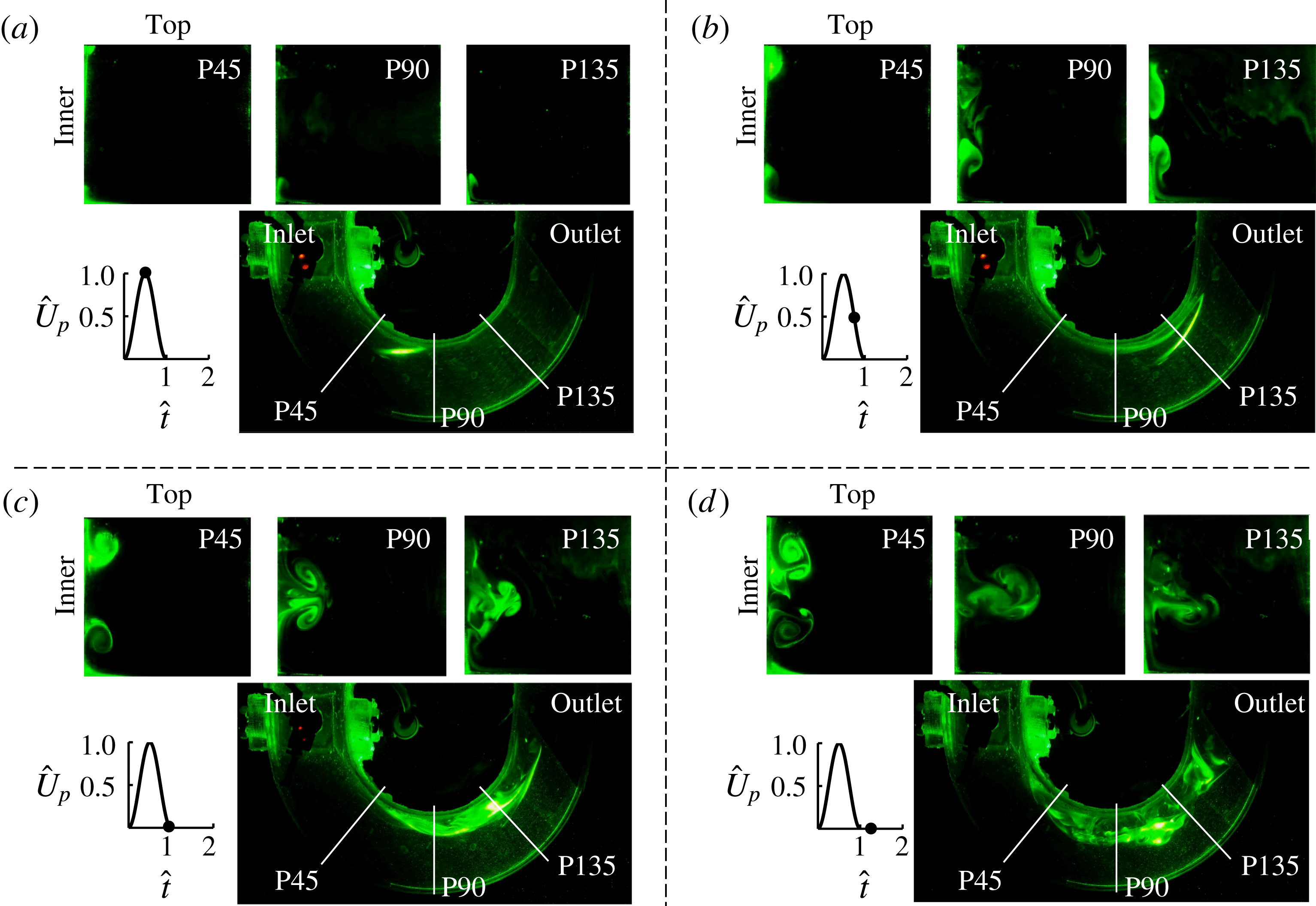
We present results from flow visualizations and numerical simulations corresponding to physiological flow (case 2) in the ascending aorta. The velocity pulse has a variation given by (2.1) and shown in figure 1(b). Figure 3 shows visualizations from experiments in the medial (
 $r{-}\unicode[STIX]{x1D703}$
) plane and those in each of the three cross-sectional (
 $r{-}z$
) planes marked P45, P90 and P135. The individual panels in the figure indicate time points corresponding to maximum piston velocity (figure 3
a), maximum deceleration (figure 3
b), end of the cycle (figure 3
c) and after stop of the piston (figure 3
d). The dye moves tangentially along the inner wall in the medial (
 $r{-}\unicode[STIX]{x1D703}$
) plane (figure 3
a) until the time corresponding to the maximum piston velocity. During the deceleration phase (figures 3
b and 3
c), we observe a large separated flow region along the inner wall which subsequently propagates radially outward and is accompanied by rapid mixing of the dye after stop of the piston (see movie 1; movies of results from experimental flow visualization and axial velocity contours from numerical simulations are provided for cases 1–3 in the accompanying supplementary material available at https://doi.org/10.1017/jfm.2017.7). Visualizations in the transverse (
 $r{-}z$
) planes for each of these time points show evolution of the flow structures in the three
 $r{-}z$
planes. The flow appears to be symmetric about the medial (
 $r{-}\unicode[STIX]{x1D703}$
) plane but varies along the flow direction, as is evident in the visualizations in planes P45, P90 and P135. The small asymmetry in the structures seen in the dye visualizations may be partly due to small but inevitable differences in the volume of the dye injected at the top and bottom walls of the pipe at the beginning of the experiment. Clear differences are visible between the inner and outer walls based on the moving dye fronts. The dye moves radially along the walls and sticks very close to the bottom and top walls; it is thus hardly visible. After impinging on the inner wall, it is carried by the flow towards the medial plane where it is readily seen. At any given time, the dye fronts seen in the transverse planes move larger distances along the inner wall as we proceed from the P45 to the P135 plane. For each of these planes, the dye fronts move towards each other with increasing time. After collision in the medial (
 $r{-}\unicode[STIX]{x1D703}$
) plane, the flow structures move radially outward (figures 3
b and 3
c). The time at which the collision occurs decreases as
 $\unicode[STIX]{x1D703}$
increases; for example, at
 $\hat{t}=1$
(figure 3
c) the structures have already collided in the P90 and P135 planes but are still apart in the P45 plane. Following the stop of the piston, there are significant distortions in these structures, which are clearly seen in both the transverse and medial plane visualizations (figure 3
d). In the following sections, we will show that the radial inward flow on the top and bottom walls is essentially a wall jet caused by centrifugal forces.
Experimental flow visualizations are shown for case 2 (
 $Re\sim 3842$
and
 $\hat{\unicode[STIX]{x1D6FF}}\sim 0.29$
; table 3) at (a) maximum velocity, (b) maximum deceleration, (c) end of pulse and (d) after stop of piston (
 $\hat{t}=1.25$
). The three transverse
 $(r{-}z)$
planes (P45, P90 and P135) and the medial
 $(r{-}\unicode[STIX]{x1D703})$
plane in each panel highlight the evolution in the flow structures.

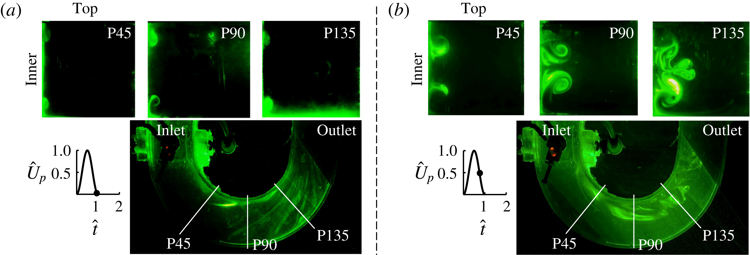
To see the effect of change of the pulse width on the flow structure, we present results corresponding to two points in the regime map (figure 2) that have the same values of
 $Re$
(
 $=3622$
) but different pulse widths; these points are marked by a triangle and a square in figure 2 and correspond to cases 1 and 3 in table 3. Case 1, with twice the time period of the physiological case, has a larger boundary layer thickness
 $\hat{\unicode[STIX]{x1D6FF}}$
(
 ${\sim}0.41$
) and larger flow travel
 $\hat{L}$
(
 ${\sim}5.6$
); case 3, with half the physiological time period, has smaller
 $\hat{\unicode[STIX]{x1D6FF}}$
(
 ${\sim}0.2$
) and smaller
 $\hat{L}$
(
 ${\sim}1.4$
) (table 3). Figure 4 shows visualizations at the end of the cycle (
 $\hat{t}=1$
) for case 1 and at maximum deceleration time (
 $\hat{t}=0.75$
) for case 3. We see similar structures to those in figure 3 but with some differences. Specifically, even at the end of the pulse, for the shorter pulse width (figure 4
a), these structures have moved very little from the top and bottom walls towards the medial (
 $r{-}\unicode[STIX]{x1D703}$
) plane. In contrast, for the longer pulse width (figure 4
b), the vortices reach and collide at the midplane even before the end of the pulse. The plane P135 shows intense mixing caused by interactions of the secondary flow structures for the longer pulse width case. In the medial plane, the dye streaks remain intact for the shorter pulse width case (figure 4
a), whereas flow separation is clearly visible for the case with longer pulse width (case 1, figure 4
b) (see movies 2 and 3).
Visualizations showing the effect of pulse width on secondary flow structures. (a) Case 3,
 $Re\sim 3622$
and
 $\hat{\unicode[STIX]{x1D6FF}}\sim 0.2$
, with half the pulse width; (b) case 1,
 $Re\sim 3622$
and
 $\hat{\unicode[STIX]{x1D6FF}}\sim 0.41$
, with twice the pulse width.

3.2 Results from numerical simulations
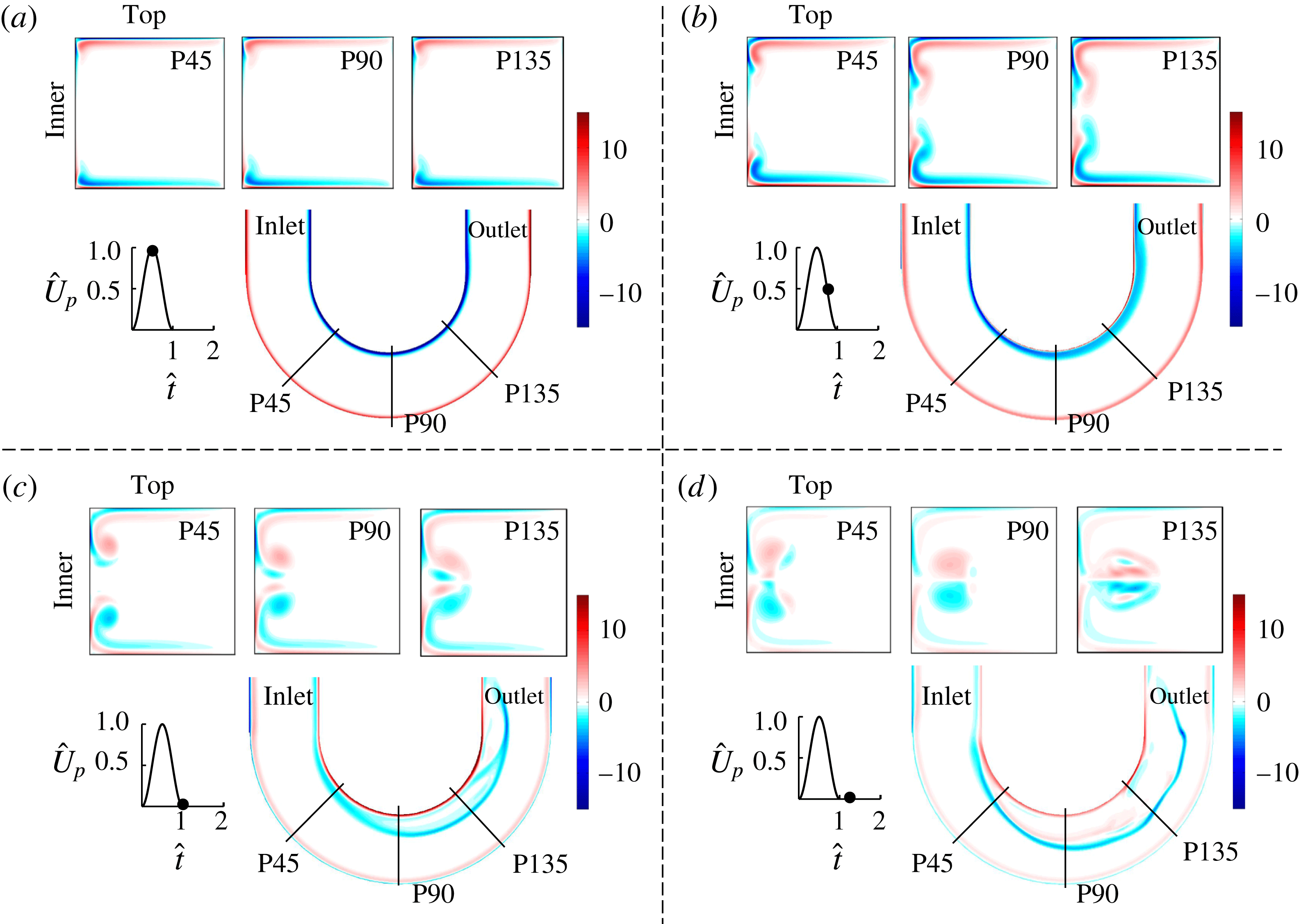
Flow visualizations are mainly useful in providing qualitative information on the various structures, whereas numerical simulations enable us to quantify the flow physics. Results from simulations for physiological flow (case 2) are shown in figure 5 in the two planes at the four time points shown earlier (figure 3). At the maximum piston velocity (
 $\hat{t}=0.5$
), in the three transverse (
 $r{-}z$
) planes, a vorticity layer appears along the top and bottom walls of the tube and ends near the inner wall corners. At this time, vorticity is confined to the inner and outer walls in the medial (
 $r{-}\unicode[STIX]{x1D703}$
) plane. At the maximum deceleration point (
 $\hat{t}=0.75$
), the vorticity in the transverse plane is transported along the inner wall towards the medial plane, where the fronts are seen as two vortex pairs in figure 5(b); these displacements increase in magnitude as we move from P45 to P135. At
 $\hat{t}=1.00$
, these vortical structures become more prominent and also collide in the transverse planes P90 and P135. After collision, these structures move radially outward into the core. This radially outward movement of vorticity is also clearly visible in the medial plane (figure 5
c). At
 $\hat{t}=1.25$
, the collision is also present in plane P45. The numerical simulations agree well with the visualizations in figure 3 for cases where the structures are orderly before the stop of the piston. They do not, however, capture the complex mixing observed in the experimental visualizations at later times, for example P90 and P135 at
 $\hat{t}=1.25$
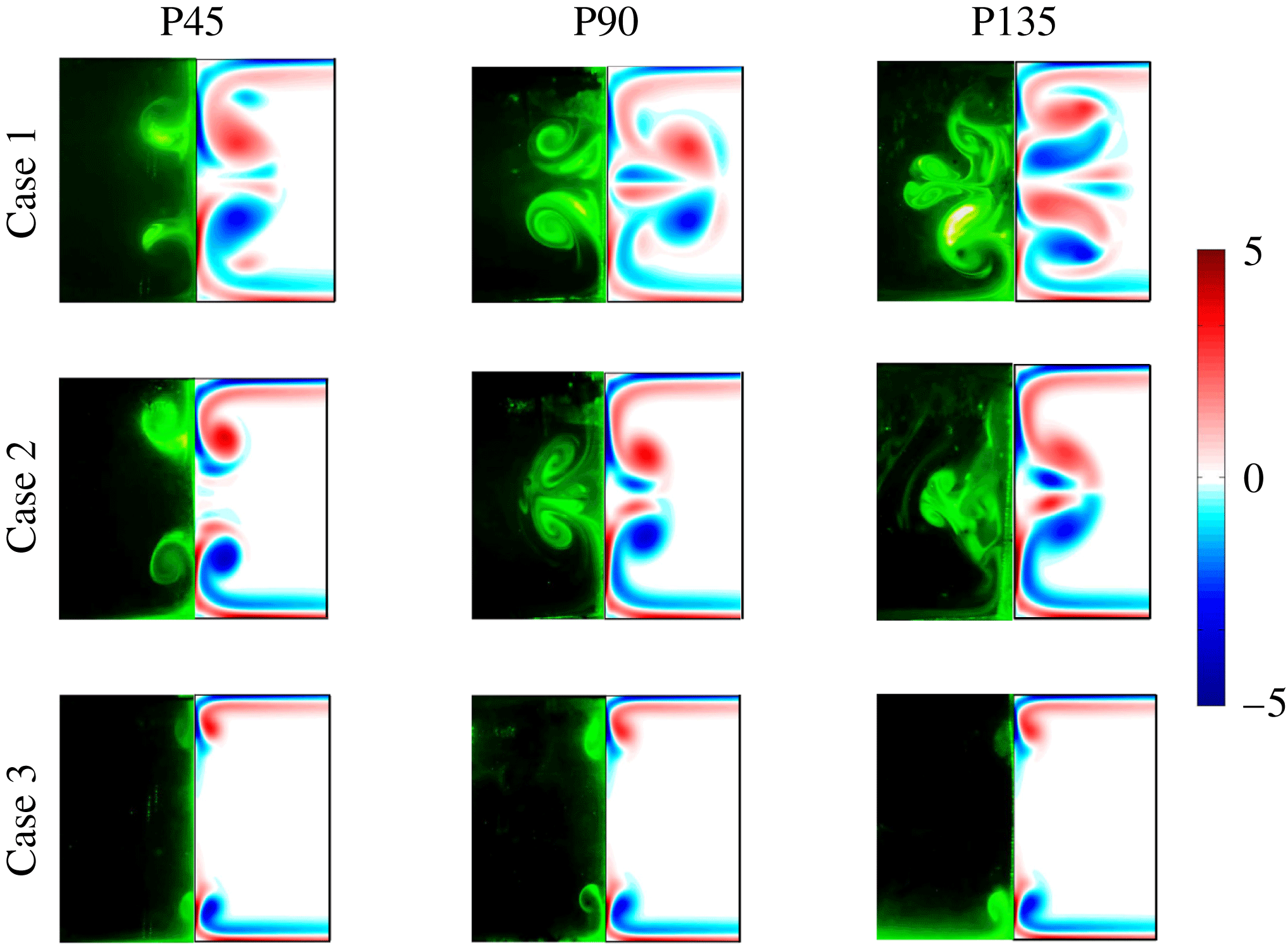
. Figure 6 shows comparisons of flow visualizations and vorticity contours for cases 1–3 at the end of the time pulse. The locations and shapes of the vortical structures from the experiments and simulations match well until collision. After collision, details of the substructures are not captured in the simulations although the overall structures appear similar, as is clearly visible for the P135 plane corresponding to cases 1 and 2.
Spatio-temporal variations in the vorticity, normalized by
 $U_{p(max)}/a$
, are shown from numerical simulations for case 2 at times corresponding to (a)
 $\hat{t}=0.5$
, (b)
 $\hat{t}=0.75$
, (c)
 $\hat{t}=1.00$
and (d)
 $\hat{t}=1.25$
. These are similar to the results from flow visualization experiments (figure 3).

Experimental flow visualization results are shown on the left half of each panel and the vorticity contours are shown on the right half. The results are for cases 1–3 in the three transverse planes at the end of the time pulse.

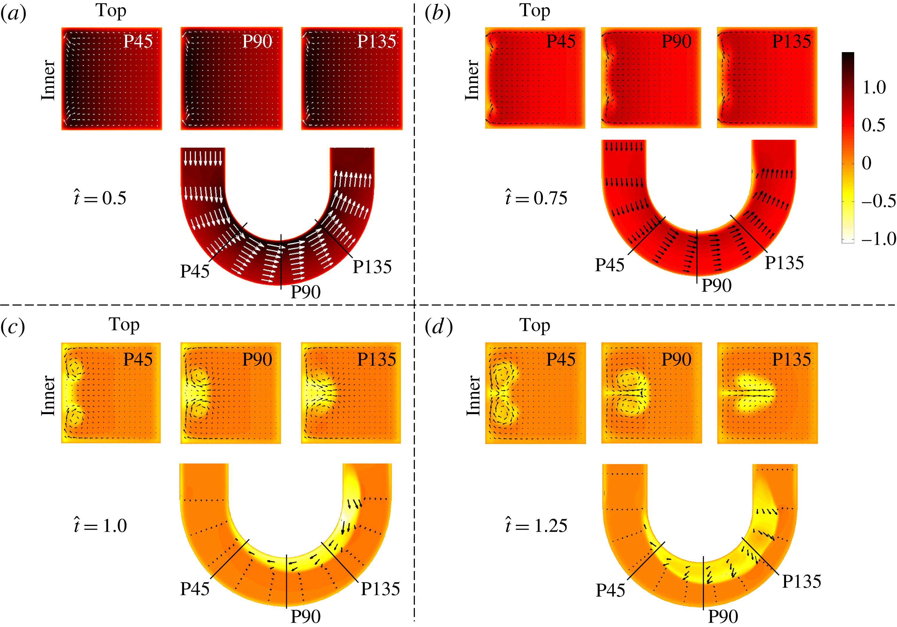
Velocity vectors superimposed on normalized axial velocity contours from numerical simulation for case 2 at different time points in the cycle. The reverse flows get trapped in these vortices which subsequently advance radially.

Figure 7 shows the normalized axial velocity contours from the numerical simulations for case 2. Also superimposed on this figure are the velocity vectors, in both the medial (
 $r{-}\unicode[STIX]{x1D703}$
) and transverse (
 $r{-}z$
) planes. As is evident from the vorticity contours (figure 5), the flow consists of two regions: an inviscid core, and viscous or vorticity layers that are initially confined to near the walls of the tube. At
 $\hat{t}=0.5$
, which corresponds to the point of maximum piston velocity, the uniform velocity profile in the medial (
 $r{-}\unicode[STIX]{x1D703}$
) plane at the inlet gets rapidly skewed as the flow enters the curved section. This skewing is due to the centrifugal effects, with maximum velocity occurring near the inner wall. The boundary layers are barely visible in this figure as very thin regions near the walls that have thickness proportional to
 $\sqrt{\unicode[STIX]{x1D708}t}$
. Further, at this time, the axial velocity distributions in the transverse planes (P45, P90, and P135) are nearly the same. At peak deceleration (
 $\hat{t}=0.75$
), the average velocity is halved but has a similar skewed profile in the medial plane, as seen in figure 7(a). In the transverse planes, however, there are distinct low-velocity regions near the inner wall; these regions almost coincide with the dye fronts (figure 3
b) and with the vortex pairs in figure 5(b). The axial velocity averaged over the cross-section in each transverse plane is zero after stop of the piston (figures 7
c and 7
d). We observe small positive axial velocities over a significant region of the transverse planes, with the development of large reverse flows in regions located near the inner wall. It should be noted that these reverse flow regions again coincide with the vortical structures in the transverse planes (compare figures 5 and 7 at
 $\hat{t}=1$
). The growth of reverse flow regions is clearly visible in the medial planes (figures 7
c and 7
d). The velocity vectors in the transverse planes also clearly show the vortical regions corresponding to the visualizations (figure 3) and to the vorticity contour plots (figure 5). Large flow separations are present only near the inner wall; in contrast, reverse flows are confined to thin boundary layers on the other three walls. The separated reverse flow region is highly three-dimensional and varies both along the flow direction and over time.
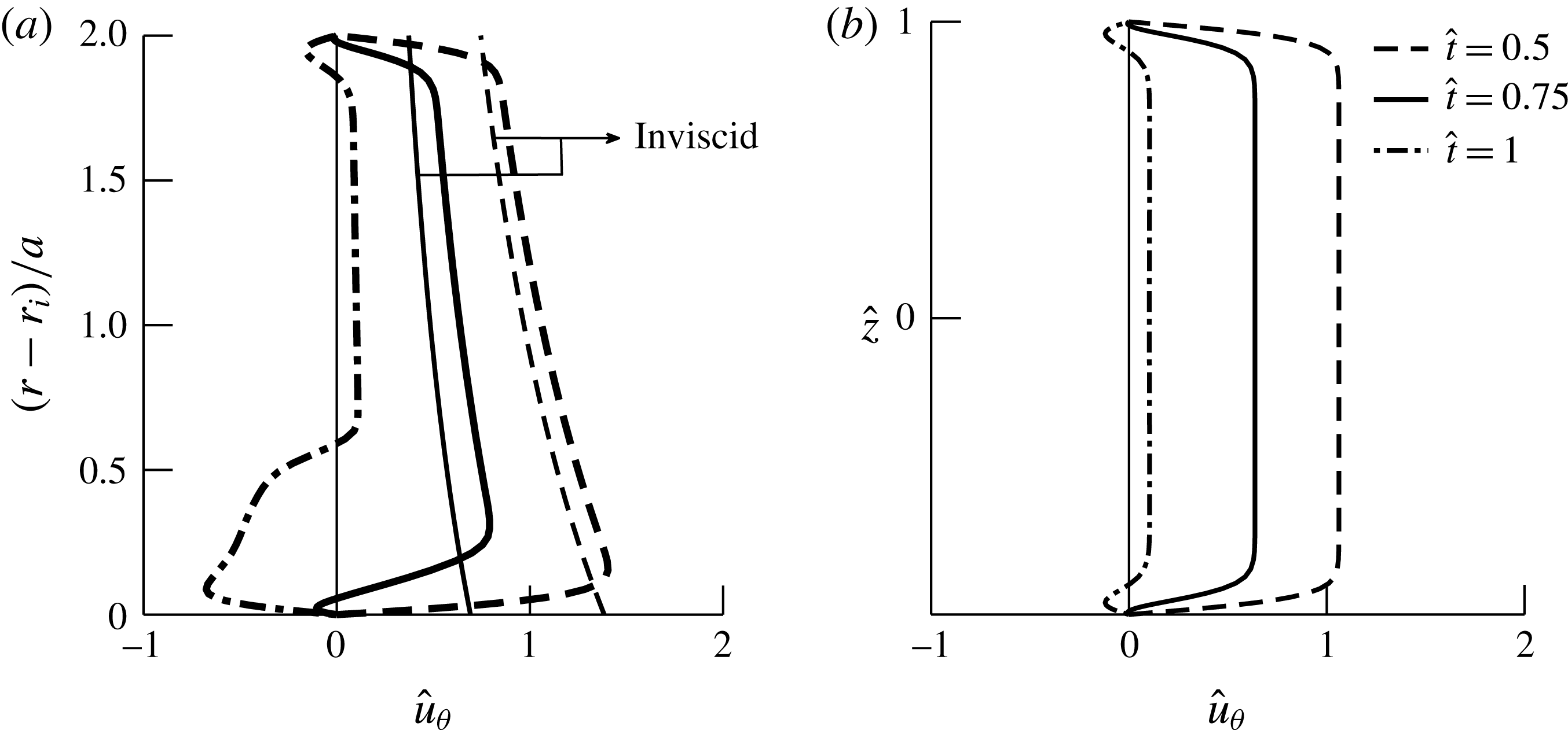
To further quantify these flow features, we show the axial velocity profiles at three different time points for the P90 plane from the inner to the outer wall (figure 8
a) and the axial velocity profiles along the
 $z$
-direction from the bottom to the top walls (figure 8
b). At maximum piston velocity (
 $\hat{t}=0.5$
), we observe a skewed velocity profile in the inviscid core and boundary layers at the wall. Small reverse flow regions are observed near the inner and outer walls at the maximum deceleration point (
 $\hat{t}=0.75$
). At
 $\hat{t}=1$
, the velocity profile with radial distance (figure 8
a) shows large reverse flow regions near the inner wall and a small positive velocity in the inviscid core. The velocity profiles with
 $\hat{z}$
show constant velocities in the inviscid core with small reverse flow regions developing in the boundary layers over time.
(a) Axial velocity profiles from numerical simulations for case 2, in the plane P90 and the medial
 $(r{-}\unicode[STIX]{x1D703})$
plane at
 $\hat{z}=0$
, for three different times. The inviscid velocity, calculated from potential flow in an annulus, is superimposed on the plot. (b) Variation of the axial velocity
 $\hat{z}$
(
 $=z/a$
) is shown at
 $(r-r_{i})/a=1$
.

These results show that the secondary flow, having a wall-jet-type profile, is initially present on the top (or bottom) walls, gains in strength with time, and impinges on the inner wall. Subsequently, the two wall jets from the top and bottom halves collide in the midplane and form a re-entrant jet from the inner to the outer wall.
3.3 Secondary flow causes separation
Classical unsteady boundary layer separation, for example on an impulsively started bluff body (see Koumoutsakos & Leonard Reference Koumoutsakos and Leonard1995; Das, Srinivasan & Arakeri Reference Das, Srinivasan and Arakeri2013b ) or on an airfoil with a rapidly changing angle of attack leading to dynamic stall (Currier & Fung Reference Currier and Fung1992; Shih et al. Reference Shih, Lourenco, Van Dommelen and Krothapalli1992), is essentially a two-dimensional phenomenon which occurs due to an adverse pressure gradient. The boundary layer, and vorticity, formerly attached to the surface, move away from it, accompanied by breakdown of the boundary layer assumption. It should be noted that the presence of reverse flow does not imply separation, although a separated layer often contains reverse flow regions: the reverse flow region can be thin and the boundary layer assumption is still valid. There are no simple criteria to identify unsteady boundary layer separation, unlike in steady separation where it is very close to the point of zero WSS. The Moore–Rott–Sears (MRS) criterion has been proposed to identify unsteady boundary layer separation, but requires information that is not easily available. Analytically, a singularity in the boundary layer equation is found when an unsteady boundary layer separates (Van Dommelen & Shen Reference Van Dommelen and Shen1980; Van Dommelen & Cowley Reference Van Dommelen and Cowley1990). This singularity can be interpreted as an unbounded expansion of a slug of fluid in the direction normal to the boundary layer from a Lagrangian frame of reference (Cowley, Van Dommelen & Lam Reference Cowley, Van Dommelen and Lam1990).
In the case of the unsteady flow in a curved tube in this study, we see breakdown of the boundary layer assumption (moving of vorticity away from the surface) on the inner curved wall. This separation is due to the three-dimensional nature of the flow and may or may not have reverse flow. We need to consider the flow in the transverse
 $(r{-}z)$
plane first to understand the process of separation on the inner wall in the medial
 $(r{-}\unicode[STIX]{x1D703})$
plane. The two boundary layers (wall jets) ‘separate’ when they collide in the medial plane on the inner wall (e.g. figure 3
b, P90 plane), and can be considered as due to the formation of a singularity in the boundary layer equations (Stewartson et al.
Reference Stewartson, Cebeci and Chang1980; Riley Reference Riley1998). This collision also causes separation of the boundary layer in the medial
 $(r{-}\unicode[STIX]{x1D703})$
plane, in that the
 $\unicode[STIX]{x1D714}_{z}$
(component of vorticity normal to the medial
 $(r{-}\unicode[STIX]{x1D703})$
plane) vorticity moves away from the inner wall due to collision. The boundary layer
 $\unicode[STIX]{x1D714}_{z}$
vorticity is advected by the secondary flow initiated on the straight walls. Thus, the separation is due to the secondary flow and not due to an adverse pressure gradient as is the case in classical separation. Moreover, the separated region may or may not have reverse flow. If the collision occurs in the acceleration phase itself, there will be no reverse flow in the medial
 $(r{-}\unicode[STIX]{x1D703})$
plane. However, flow does reverse during the deceleration phase (when the temporal adverse pressure gradient is negative); the low-momentum fluid carried by the secondary flow reverses direction. A deceleration phase is, however, not required for separation, only for flow reversal. For case 2, collision in the P135 plane occurs at around
 $\hat{t}\sim 0.8$
, and the axial flow in the boundary layer has reversed direction (see figure 7 and movie 1). For case 3, however, the secondary flow does not collide in the medial plane although there are reverse flows present in the boundary layer (see figure 4
a and movie 2).
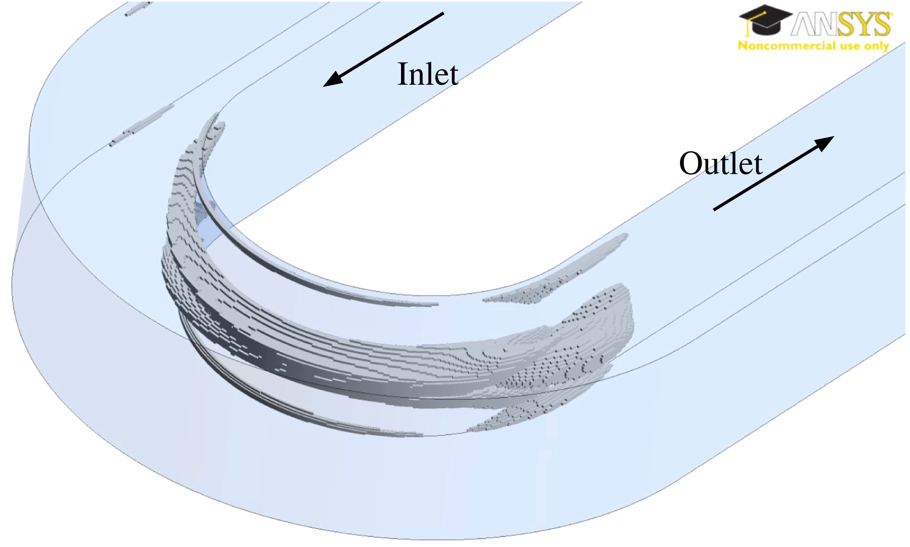
Isocontour surfaces, corresponding to
 $\hat{u} _{\unicode[STIX]{x1D703}}=-0.4$
, at
 $\hat{t}=1$
, showing the 3D separated flow region near the inner wall. The results are from numerical simulations for case 2.

Figure 9 shows the three-dimensional structure of the separated flow for case 2 on the inner wall of the tube at the end of the pulse,
 $\hat{t}=1$
. The surface is an isocontour corresponding to the axial velocity,
 $\hat{u} _{\unicode[STIX]{x1D703}}=-0.4$
, obtained from the numerical results, with cross-sections corresponding to the contours in figure 7. The separated region develops at the end of the curvature and propagates upstream with time. This separated region is due to accumulation of the low-momentum boundary layer fluid near the inner wall, which reverses direction during the deceleration phase of the cycle. The reverse flow velocities in this region are high and of the order of 40 % of the maximum piston velocity. In addition, there are other smaller reverse flow regions in the boundary layers, with lower velocities, on the other three walls, which would appear for a choice of lower contour level (figures 7 and 8).
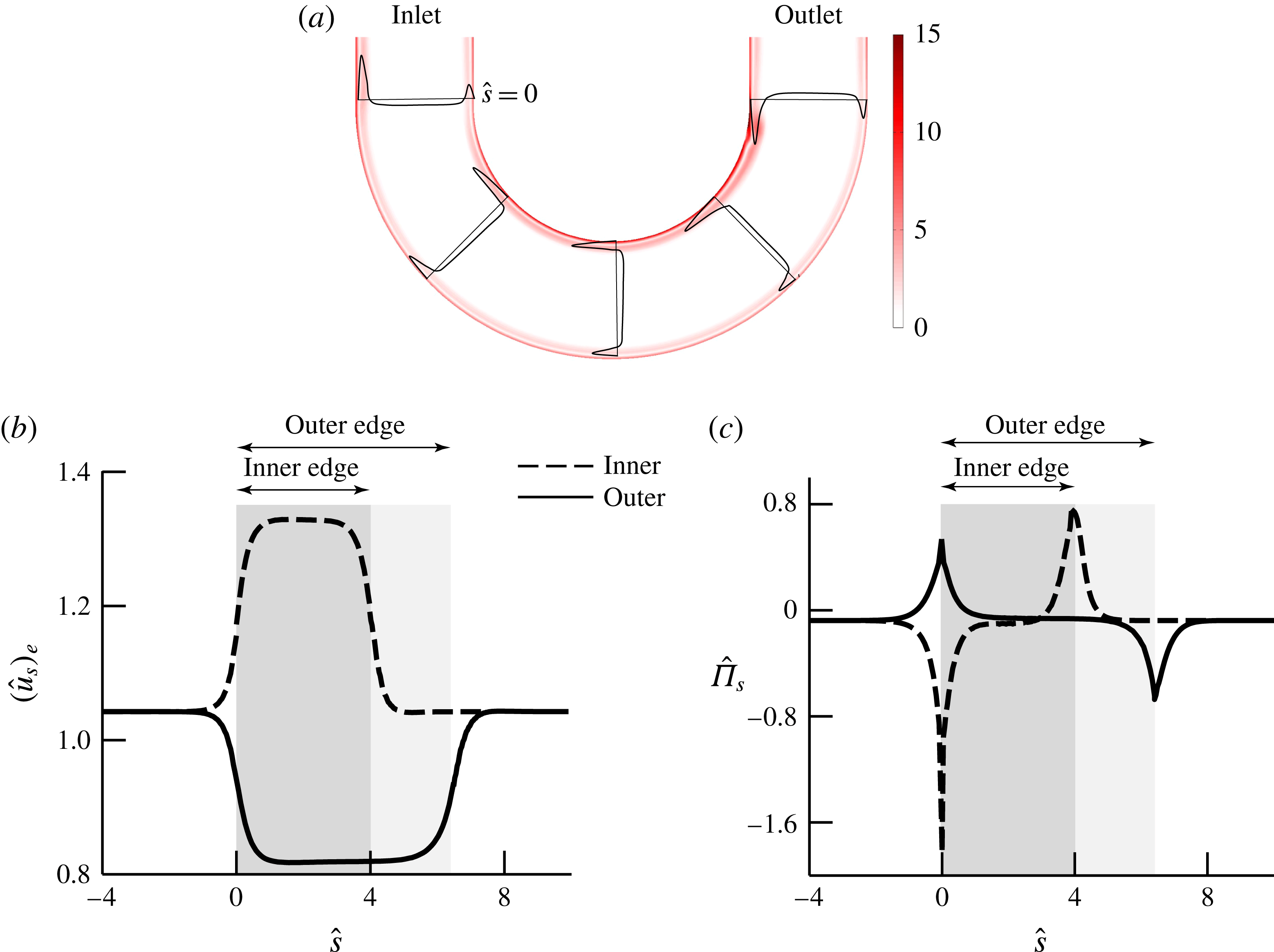
(a) Normalized vorticity magnitude contours are shown for a 2D numerical simulation corresponding to case 2 at
 $\hat{t}=1$
. The axial velocity profiles are shown at five planes. Variations in (b) the streamwise velocity,
 $(\hat{u} _{s})_{e}$
, and (c) the streamwise pressure gradient,
 $\hat{\unicode[STIX]{x1D6F1}}_{s}$
, normalized by
 $(1/2)\unicode[STIX]{x1D70C}U_{p(max)}^{2}/(2a)$
, are shown with the non-dimensional streamwise coordinate,
 ${\hat{s}}$
, at the edge of the boundary layer along the inner (dashed) and outer walls (solid) at
 $\hat{t}=0.5$
. The beginning of the streamwise coordinate
 ${\hat{s}}=0$
is at the start of the curved section at the inlet. The shaded region indicates the curved section.

The importance of secondary flow in causing this large separated flow is clear when we consider 2D flows in a planar curved geometry subjected to the same unsteady flow pulse. Figure 10 shows the normalized vorticity magnitude contours at the end of the pulse for the same input velocity profile. We see the presence of reverse flow in the boundary layers over most of the curved regions of the tube due to the deceleration of the piston; these layers have, however, not separated. The magnitude of the reverse axial velocity near the inner wall in the 3D case is 86 % higher than that obtained in the 2D simulation. To analyse further, it is useful to split the boundary layer pressure gradient into two parts: spatial (
 $\unicode[STIX]{x1D6F1}_{s}$
) and temporal (
 $\unicode[STIX]{x1D6F1}_{t}$
) components, as given by (3.1) (Das et al.
Reference Das, Srinivasan and Arakeri2016):
 $$\begin{eqnarray}\frac{\unicode[STIX]{x2202}p(s,t)}{\unicode[STIX]{x2202}s}=\underbrace{\unicode[STIX]{x1D70C}\frac{\unicode[STIX]{x2202}(u_{s})_{e}}{\unicode[STIX]{x2202}t}}_{\unicode[STIX]{x1D6F1}_{t}}+\underbrace{\unicode[STIX]{x1D70C}(u_{s})_{e}\frac{\unicode[STIX]{x2202}(u_{s})_{e}}{\unicode[STIX]{x2202}s}}_{\unicode[STIX]{x1D6F1}_{s}},\end{eqnarray}$$
where
 $(u_{s})_{e}$
is the streamwise velocity at the edge of the boundary layer and
 $s$
is the streamwise coordinate. The first part
 $(\unicode[STIX]{x1D6F1}_{t})$
is due to the temporal acceleration of the inviscid flow at the edge of the boundary layer; the spatial part
 $(\unicode[STIX]{x1D6F1}_{s})$
is due to the convective acceleration. Figures 10(b) and 10(c) show variations in the streamwise coordinate of the velocity (
 $(\hat{u} _{s})_{e}$
) and the spatial pressure gradient (
 $\hat{\unicode[STIX]{x1D6F1}_{s}}$
). The variations are shown at the inner (dashed line) and outer walls (solid line). These figures clearly show regions of favourable and adverse pressure gradients for the spatial component in the curved pipe. The variations for the 3D case for the streamwise velocity and the pressure gradients are very similar. Over most of the curved section,
 $\hat{\unicode[STIX]{x1D6F1}}_{s}$
is nearly 0. There are adverse pressure gradients (
 $\hat{\unicode[STIX]{x1D6F1}}_{s}>0$
) only on the outer wall near the inlet and the inner wall near the outlet (figure 10
c). These regions correspond to locations where both the spatial and temporal components contribute to the adverse pressure gradient. We can see in figure 10(a) that these spatial adverse pressure gradients are mild and there is only a small thickening of the boundary layer on the inner wall near the outlet. These features may be seen in the velocity profiles which are superimposed and shown in figure 10(a) at the inlet, P45, P90, P135 and the outlet plane. The separation seen on the inner wall in the 3D case, clearly different from that in the 2D case, is due to accumulation of low-momentum fluid due to the secondary flow which is absent in the 2D case.
4 On the origin of secondary flows and separations
When a fluid enters a curved pipe from a reservoir, the flow field at initial times comprises an inviscid potential core and viscous boundary layers near the walls, as discussed earlier. In the potential core, the radial pressure gradient is balanced by the centrifugal force and is given as
 $$\begin{eqnarray}-\frac{\unicode[STIX]{x2202}P(r,\unicode[STIX]{x1D703},t)}{\unicode[STIX]{x2202}r}+\frac{\unicode[STIX]{x1D70C}u_{\unicode[STIX]{x1D703}(\mathit{invis})}^{2}}{R}=0,\end{eqnarray}$$
where
 $u_{\unicode[STIX]{x1D703}(\mathit{invis})}$
represents the axial velocity in the inviscid core. The expression for
 $u_{\unicode[STIX]{x1D703}(\mathit{invis})}$
is given in appendix A. This pressure gradient is imposed on the top and bottom wall boundary layers flows in the radial direction. This forcing term induces a radially inward flow, the secondary flow, on the top and bottom walls. The momentum equation for the boundary layer in the radial direction is
 $$\begin{eqnarray}\frac{\unicode[STIX]{x2202}u_{r}}{\unicode[STIX]{x2202}t}+u_{r}\frac{\unicode[STIX]{x2202}u_{r}}{\unicode[STIX]{x2202}r}+\frac{u_{\unicode[STIX]{x1D703}}}{r}\frac{\unicode[STIX]{x2202}u_{r}}{\unicode[STIX]{x2202}\unicode[STIX]{x1D703}}+u_{z}\frac{\unicode[STIX]{x2202}u_{r}}{\unicode[STIX]{x2202}z}=-\left(\frac{u_{\unicode[STIX]{x1D703}(\mathit{invis})}^{2}}{r}-\frac{u_{\unicode[STIX]{x1D703}}^{2}}{r}\right)+\text{viscous terms}.\end{eqnarray}$$
In this equation, we have replaced the pressure gradient term by
 $\unicode[STIX]{x1D70C}u_{\unicode[STIX]{x1D703}(\mathit{invis})}^{2}/R$
using (4.1). The
 $u_{\unicode[STIX]{x1D703}}^{2}/r$
term comes from solution of the boundary layer equation in the
 $\unicode[STIX]{x1D703}$
-direction on the top and bottom walls. These boundary layers have axial velocities smaller than the inviscid value (
 $u_{\unicode[STIX]{x1D703}}<u_{\unicode[STIX]{x1D703}(\mathit{invis})}$
) (figure 8
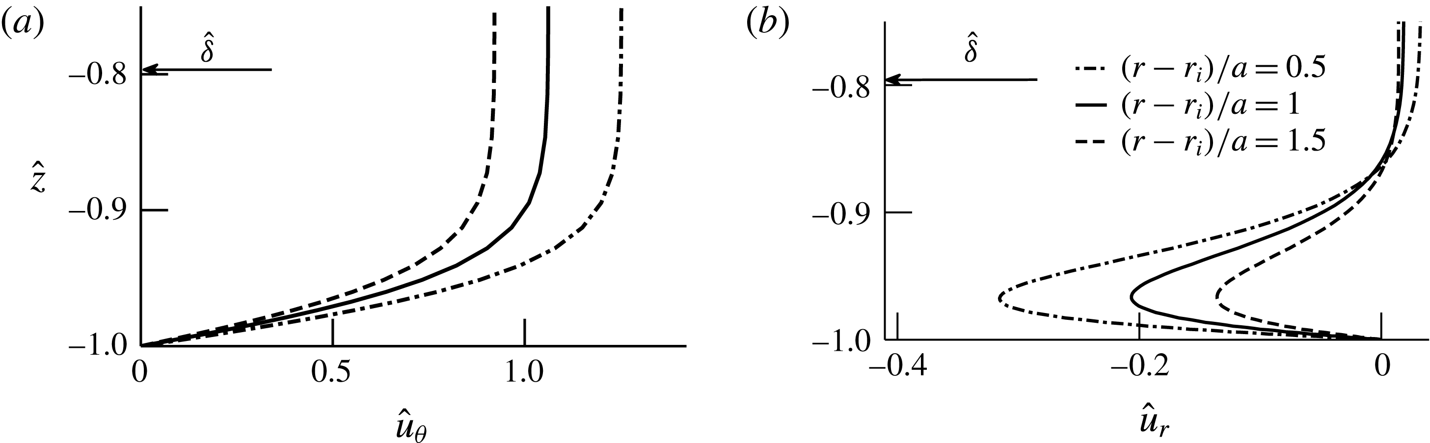
b). Thus, the first term on the right-hand side represents an imbalance between the radial pressure gradient and the centrifugal force, and is responsible for the wall-jet-type secondary flow seen on the top and bottom walls. This term varies in magnitude with time and also has radial dependence. Figure 11(a) shows normalized axial velocity profiles from the numerical simulations at three different radial locations at
 $\hat{t}=0.5$
; the value at the edge of the boundary layer corresponds to
 $u_{\unicode[STIX]{x1D703}(\mathit{invis})}$
. The maximum reached by each profile is different due to velocity skewing towards the inner wall, leading to radial dependence of the forcing term. Figure 11(b) shows the secondary flow velocity profiles, at the same radial locations as in figure 11(a), and at the same time (
 $\hat{t}=0.5$
). The forcing term is maximum at the inner wall, which leads to higher values of the radial velocity at
 $(r-r_{i})/a=0.5$
. Thus, the lower axial velocities in the top and bottom boundary layers lead to a pressure imbalance, which in turn causes the radially inward secondary flow. The secondary flow velocity profiles are in the form of a wall jet and are akin to those observed next to a vertically heated plate in still fluid. The changes in density due to temperature difference induce a body force and cause a wall-jet-like flow.
(a) Axial velocity profiles are shown from numerical simulations for case 2 in the plane P90 at three different radial locations at
 $\hat{t}=0.5$
. The normalized boundary layer thickness
 $\hat{\unicode[STIX]{x1D6FF}}$
is indicated by an arrow. (b) The corresponding radial velocity profiles show a radially inward increase in the secondary flow strength.

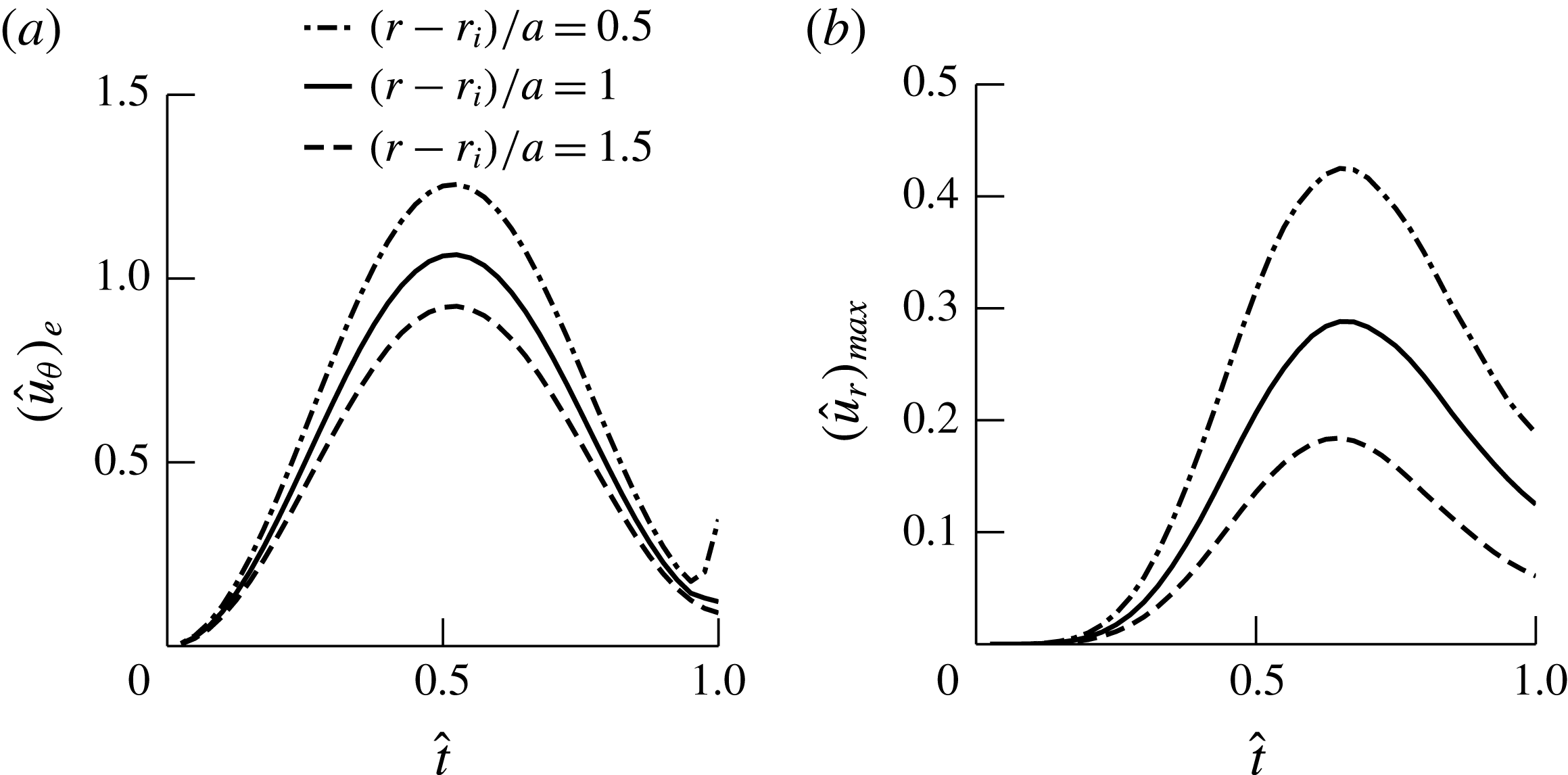
Temporal evolution of the normalized (a) axial velocity, at the edge of the boundary layer, and (b) radial velocity, in the plane P90, at three radial locations, from numerical simulations for case 2.

We next explored temporal variations of the secondary flow at the same three radial locations as in figure 11. Figure 12(a) shows variations with time of the inviscid axial velocities adjacent to the boundary layer corresponding to the plane P90 with time. This variation in
 $(u_{\unicode[STIX]{x1D703}})_{e}$
directly changes the magnitude of the forcing term in (4.2), which causes secondary flows in the boundary layers on the top and bottom walls of the tube. The corresponding variations in the maximum radial flow velocity are shown in figure 12(b). These results show a temporal shift in the maxima between the radial and axial components of the velocities, which may be due to the combined effects of convective acceleration and the viscous terms in the radial momentum balance equation (4.2). The secondary flow velocities are very small until approximately
 $\hat{t}=0.2$
and rapidly increase subsequently. It should be noted that the magnitude of the secondary flow velocity reaches approximately 40 % of the peak piston velocity at
 $(r-r_{i})/a=0.5$
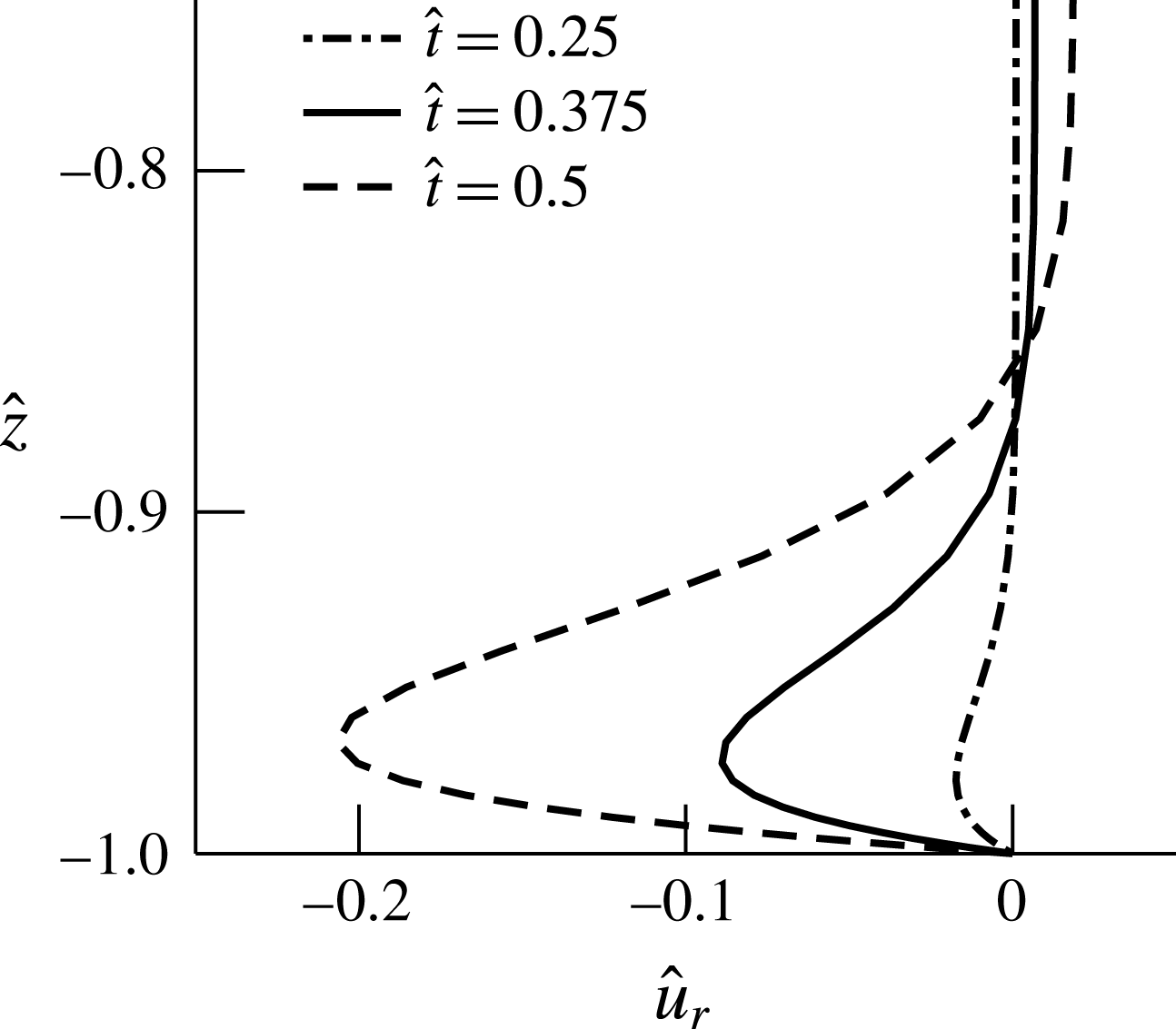
. Figure 13 shows profiles of the radial velocity in the midplane at different times up to the maximum velocity point.
Radial flow velocity profiles are shown for the plane P90 at
 $(r-r_{i})/a=1$
for different times corresponding to case 2 from numerical simulations.

4.1 Scaling relations for the secondary flow velocity
There is a balance of the centrifugal forces and radial pressure gradient in the inviscid core, which is given by (4.1). As we have seen above, this pressure gradient acting in the boundary layer causes the secondary flow in the form of a wall jet on the top and bottom walls. From this balance, we obtain the expression for the secondary flow velocity
 $U_{s}$
(see appendix A for details) in terms of the tube curvature and the period of the pulse,
 $T$
, as
 $$\begin{eqnarray}U_{s}\sim \frac{1}{\unicode[STIX]{x03C0}}\frac{U_{p(max)}^{2}T}{R}\unicode[STIX]{x1D6FD}^{2}\unicode[STIX]{x1D705}^{2}.\end{eqnarray}$$
The curvature parameter,
 $\unicode[STIX]{x1D705}$
, is defined in terms of the curvature ratio,
 $\unicode[STIX]{x1D6FD}$
, as
 $\unicode[STIX]{x1D705}=1/\ln ((1+\unicode[STIX]{x1D6FD})/(1-\unicode[STIX]{x1D6FD}))$
. The secondary flow velocity
 $U_{s}$
may also be expressed in terms of
 $Re_{\unicode[STIX]{x1D6FF}}$
and
 $\hat{\unicode[STIX]{x1D6FF}}$
as
 $$\begin{eqnarray}\hat{U} _{s}=\frac{U_{s}}{U_{p(max)}}\sim \frac{1}{13.69\unicode[STIX]{x03C0}}Re_{\unicode[STIX]{x1D6FF}}\hat{\unicode[STIX]{x1D6FF}}\unicode[STIX]{x1D6FD}^{3}\unicode[STIX]{x1D705}^{2}.\end{eqnarray}$$
Maximum radial velocities,
 $u_{r}$
, in the plane P90 at
 $(r-r_{i})/a=1$
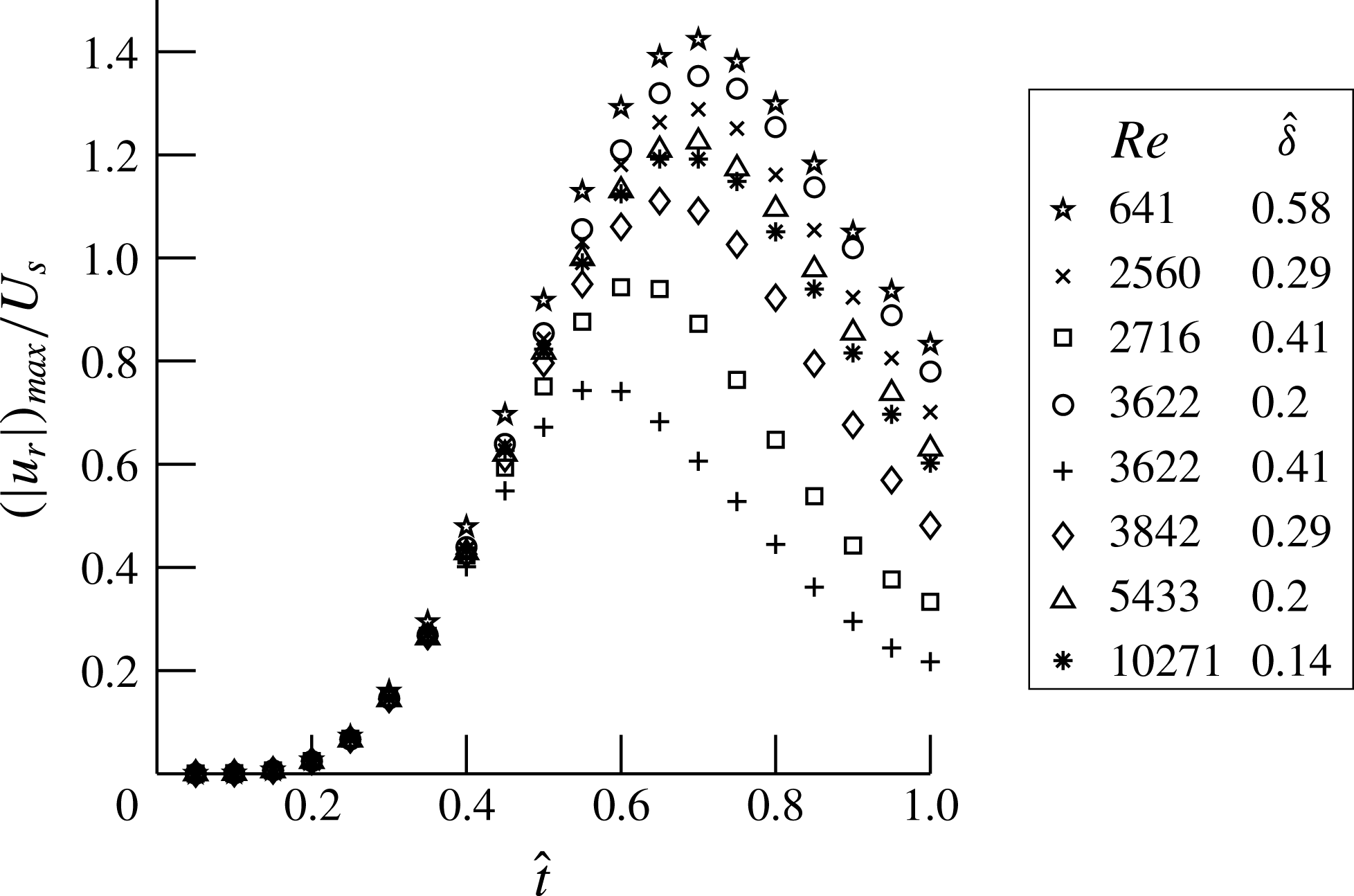
, normalized by the secondary flow velocity scale,
 $U_{s}$
(4.3), are plotted with non-dimensional time for different cases which were obtained from the numerical simulations.

In arriving at this scaling, we have assumed the flow to be fully developed. In the limit of
 $\unicode[STIX]{x1D6FD}\rightarrow 0$
, the relation for (4.3) is the velocity scale for the secondary streaming Reynolds number,
 $R_{s}$
, obtained by Lyne (Reference Lyne1971) for oscillatory fully developed flows in pipes with low curvatures. In other words,
 $R_{s}=U_{s}(2a)/\unicode[STIX]{x1D708}$
in the limit
 $\unicode[STIX]{x1D6FD}\rightarrow 0$
. Figure 14 shows the maximum radial velocity,
 $u_{r}$
, from the computational results normalized with
 $U_{s}$
. These normalized velocities are plotted versus time and were obtained for eight different values of
 $Re$
and
 $\hat{\unicode[STIX]{x1D6FF}}$
, which include the three cases listed in table 3. The secondary flow velocities are negligible until approximately
 $\hat{t}=0.2$
and then increase rapidly with time. There is reasonable collapse of the data for different combinations of
 $Re$
and
 $\hat{\unicode[STIX]{x1D6FF}}$
. We see larger deviations for the higher-
 $\hat{\unicode[STIX]{x1D6FF}}$
cases, which is especially evident at later times. This deviation for larger-
 $\hat{\unicode[STIX]{x1D6FF}}$
cases is due to breakdown of the boundary layer approximation used in the derivation of
 $U_{s}$
.
4.2 Scaling relations for motion of secondary flow structures
The secondary flow structures move towards the medial (
 $r{-}\unicode[STIX]{x1D703}$
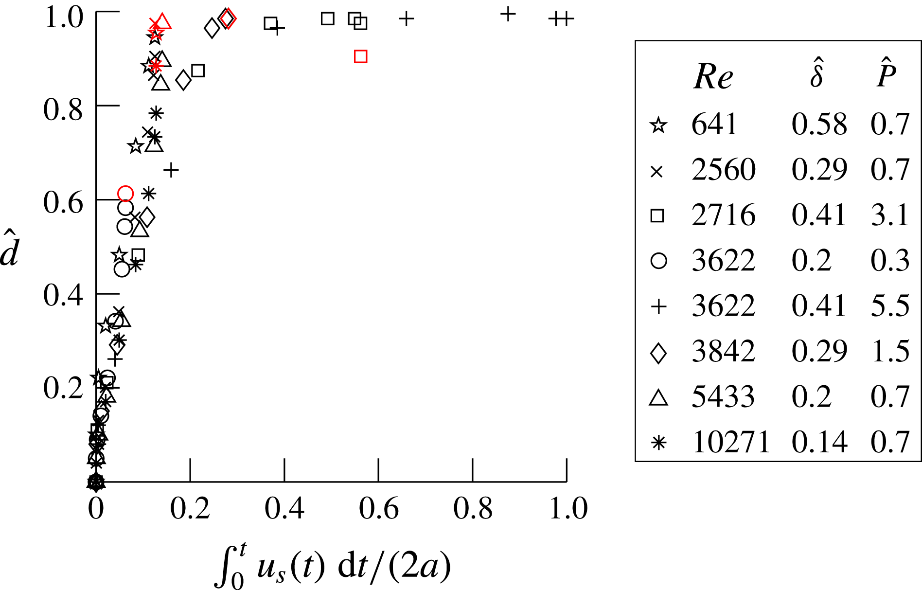
) plane after impingement on the inner wall (figures 3 and 5). Figure 15 shows the normalized distance traversed by the vorticity front
 $\hat{d}(=d/a)$
with the time-dependent integral
 $\int _{0}^{t}u_{s}(t)\,\text{d}t$
, normalized by the edge length (
 $2a$
), for the cases shown in figure 14;
 $u_{s}(t)$
is the instantaneous secondary flow velocity defined in table 2. The vorticity front corresponds to the vorticity value normalized by
 $U_{p(max)}/a=0.1$
. The time point corresponding to the end of the pulse is marked in red for each case. The normalized positions of the vorticity fronts,
 $\hat{d}$
, for cases covering a wide range of
 $Re$
–
 $\hat{\unicode[STIX]{x1D6FF}}$
values, collapse reasonably onto a single curve. In contrast to figure 14, there are no large deviations for the different cases at later times. Collision of the vorticity fronts, indicated by
 $\hat{d}=1$
, occurs at the integral value of
 ${\sim}0.2$
. The secondary velocity hence captures the movement of the vorticity fronts on the inner wall.
Variations in the normalized distance,
 $\hat{d}=d/a$
, traversed by the vorticity front are shown with the time-dependent integral
 $\int _{0}^{t}u_{s}(t)\,\text{d}t$
, normalized by the edge length (
 $2a$
), for the cases shown in figure 14. The points marked in red correspond to the end of the time pulse for each case. The end of the time pulse point corresponding to
 $Re\sim 3622$
,
 $\hat{\unicode[STIX]{x1D6FF}}\sim 0.41$
occurs at a later time, which is not shown in the figure.

We determined the distance, denoted by
 $P$
, traversed by the structures at the end of the time pulse as
 $$\begin{eqnarray}P=\int _{0}^{T}u_{s}(t)\,\text{d}t\propto U_{s}T.\end{eqnarray}$$
Substituting the secondary flow velocity scale for
 $U_{s}$
using (4.3),
 $\hat{P}$
(
 $=P/(2a)$
) can be written in terms of
 $\hat{L}$
(
 $=L/(2a)=U_{p(max)}T/(4a)$
), the average distance traversed by the fluid in the axial direction over time
 $T$
, as
 $$\begin{eqnarray}\hat{P}\sim \frac{8}{\unicode[STIX]{x03C0}}\hat{L}^{2}\unicode[STIX]{x1D6FD}^{3}\unicode[STIX]{x1D705}^{2}\end{eqnarray}$$
and in terms of
 $Re_{\unicode[STIX]{x1D6FF}}$
and
 $\hat{\unicode[STIX]{x1D6FF}}$
as
 $$\begin{eqnarray}\hat{P}\sim 8.5\times 10^{-4}Re_{\unicode[STIX]{x1D6FF}}^{2}\hat{\unicode[STIX]{x1D6FF}}^{2}\unicode[STIX]{x1D6FD}^{3}\unicode[STIX]{x1D705}^{2}.\end{eqnarray}$$
The value of
 $\hat{P}$
shows the extent of movement of the structures on the inner wall at
 $t=T$
and indicates whether collision of the structures on the inner wall has occurred at the end of the time pulse. The term
 $\unicode[STIX]{x1D705}$
is given by (A 17) and is related to the inviscid flow profile. Because
 $\unicode[STIX]{x1D6FD}$
and
 $\unicode[STIX]{x1D705}$
are constant in this study,
 $\hat{P}$
depends on
 $\hat{L}$
alone. In general, however, equation (4.6) gives the explicit dependence on
 $\unicode[STIX]{x1D6FD}$
and
 $\unicode[STIX]{x1D705}$
and can be used for tubes with any curvature.
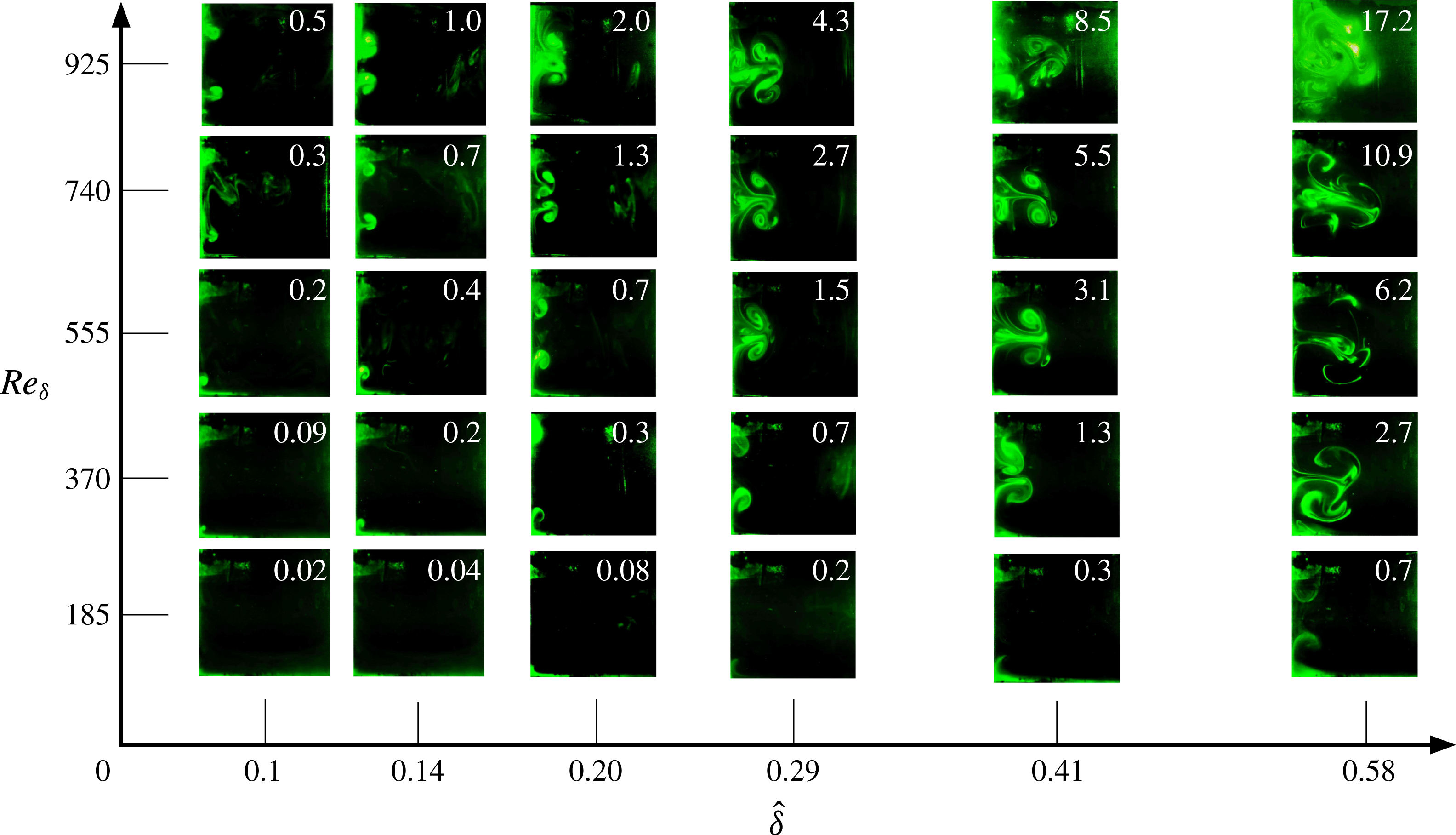
Flow visualization in the P90 plane at the end of the time pulse shown for various
 $Re_{\unicode[STIX]{x1D6FF}}$
–
 $\hat{\unicode[STIX]{x1D6FF}}$
combinations. The flow structures are similar for the same values of
 $\hat{P}$
, indicated at the top right of each panel.

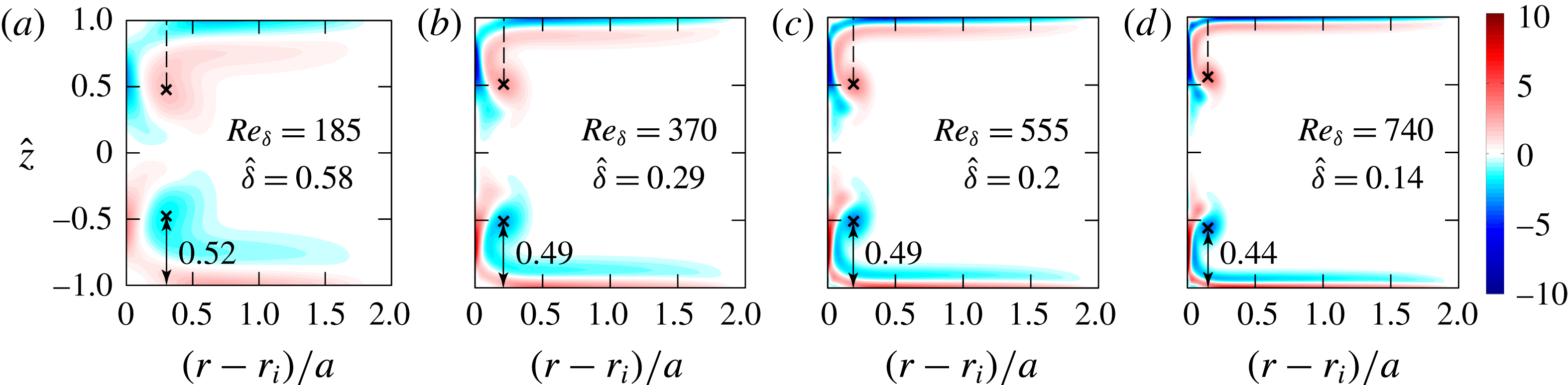
Vorticity contours, normalized by
 $U_{p(max)}/a$
, from numerical simulations corresponding to
 $\hat{P}\sim 0.7$
from figure 16. The point of maximum vorticity is indicated by
 $\times$
. The height of the maximum vorticity is approximately the same in all four cases.

Figure 16 shows the flow structures, in the plane P90 at the end of the cycle, from all of the experiments corresponding to points in the regime map (figure 2
b). The number at the top right corner of each image is the value of
 $\hat{P}$
for each case, calculated using (4.7). These visualizations show that for a given value of
 $\hat{\unicode[STIX]{x1D6FF}}$
, there is larger movement of the vortical structures on the inner wall with increasing
 $Re_{\unicode[STIX]{x1D6FF}}$
; similarly, for a given value of
 $Re_{\unicode[STIX]{x1D6FF}}$
, we see larger movements of these structures with increasing
 $\hat{\unicode[STIX]{x1D6FF}}$
. After collision at the medial (
 $r{-}\unicode[STIX]{x1D703}$
) plane, the vortical structures move radially towards the outer wall and can lead to intense mixing, as seen for the higher values of
 $Re_{\unicode[STIX]{x1D6FF}}$
and
 $\hat{\unicode[STIX]{x1D6FF}}$
. For approximately the same values of
 $\hat{P}$
in figure 16, the flow structures appear to be similar even though the
 $Re_{\unicode[STIX]{x1D6FF}}$
and
 $\hat{\unicode[STIX]{x1D6FF}}$
may be different. For example, consider the case of
 $\hat{P}\sim 0.7$
, spanning
 $Re_{\unicode[STIX]{x1D6FF}}$
from 185 to 740 and
 $\hat{\unicode[STIX]{x1D6FF}}$
from 0.14 to 0.58, which shows remarkably similar positions of the vortical structures. For low
 $\hat{P}$
values, we do not see any structures either due to the low
 $U_{s}$
values or small values of
 $T$
. In contrast, for higher values of
 $\hat{P}$
, these structures not only collide in the medial plane but also move radially towards the outer walls, as discussed earlier. To quantify the distances traversed by the flow structures, we varied the peak velocity
 $U_{p(max)}$
and pulse width
 $T$
in the input velocity profile to simulate the four cases. Results from numerical simulations in the transverse P90 plane are shown in figure 17 for the cases corresponding to
 $\hat{P}\sim 0.7$
(in figure 16). The point of maximum vorticity (indicated by
 $\times$
) is marked for each of the cases. These values vary within a small range (0.44–0.52) and correspond to a large variation in
 $Re_{\unicode[STIX]{x1D6FF}}$
(185–740) and
 $\hat{\unicode[STIX]{x1D6FF}}$
(0.14–0.58) values. We note that points corresponding to
 $\hat{P}\sim 0.7$
lie close to each other in figure 15. The
 $\hat{P}$
scaling as a measure of movement of the secondary structures is valid until the time of collision of the vortical structures in the medial plane. The secondary vortices contain low-axial-momentum fluid from the boundary layer. Thus, the outward movement after collision is, in fact, retarded compared with the stagnant fluid due to similar force imbalance to the one that created the secondary flow on the horizontal walls. Thus, for example, the flow structures for
 $\hat{P}$
values of 5.5 and 3.1, and for 4.3 and 2.7, do not look very different.
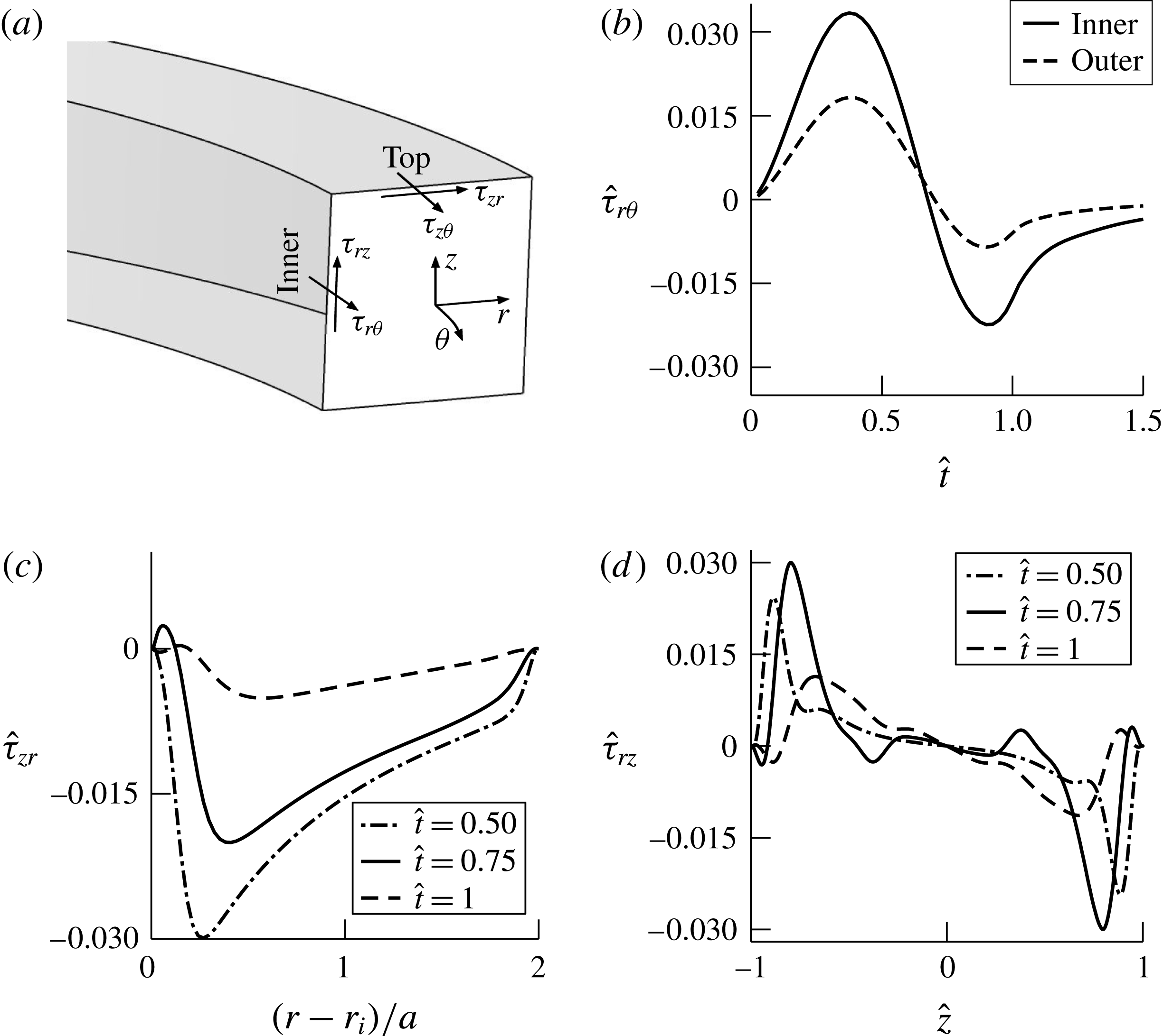
(a) Schematic showing the different components of the WSS on the walls of the tube. All WSS results are shown corresponding to the P90 plane and are for case 2 from numerical simulations. (b) Temporal variations in the
 $\hat{\unicode[STIX]{x1D70F}}_{r\unicode[STIX]{x1D703}}$
components on the inner and outer walls at
 $\hat{z}=0$
. (c) Profiles of
 $\hat{\unicode[STIX]{x1D70F}}_{zr}$
at three different times on the top wall. (d) Variations of
 $\hat{\unicode[STIX]{x1D70F}}_{rz}$
with
 $\hat{z}$
on the inner wall.

4.3 Spatio-temporal variations in the WSS components
Figure 18(a) shows a schematic of the components of the WSS in the curved tube. To assess the combined contributions of the axial and secondary flows on the WSS, we plotted the components of the WSS, normalized by the dynamic pressure
 $(1/2)\unicode[STIX]{x1D70C}U_{p(max)}^{2}$
, for the plane P90 on the inner, outer and top walls (figure 18
b–d). This type of normalization represents the skin friction coefficient, for example, corresponding to flow in a pipe. The axial WSS on the inner and outer tube walls (figure 18
b) is plotted for
 $\hat{z}=0$
, which corresponds to the medial plane. The
 $\hat{\unicode[STIX]{x1D70F}}_{r\unicode[STIX]{x1D703}}$
values on the inner wall increase to a maximum of 0.033 during the acceleration phase, and are negative, indicating flow reversal, during the deceleration phase. The values are approximately 0 at
 $\hat{t}=1.5$
, which corresponds to time periods well after the stop of the piston. The
 $\hat{\unicode[STIX]{x1D70F}}_{r\unicode[STIX]{x1D703}}$
values on the outer walls show similar variations with time but have magnitudes approximately half of those on the inner wall. Figure 18(c) shows variations of
 $\hat{\unicode[STIX]{x1D70F}}_{zr}$
in the radial direction on the top wall at three different times. These are essentially caused by the wall-jet-type secondary flows on this wall. These values are negative due to the secondary flows that are directed towards the inner wall and are skewed due to higher centrifugal forcing terms near the inner wall. The maximum in
 $\hat{\unicode[STIX]{x1D70F}}_{zr}$
is at the peak piston velocity (
 $\hat{t}=0.5$
), with magnitude similar to that of
 $\hat{\unicode[STIX]{x1D70F}}_{r\unicode[STIX]{x1D703}}$
in the axial direction. Figure 18(d) shows the corresponding variations in the
 $z$
-direction of
 $\hat{\unicode[STIX]{x1D70F}}_{rz}$
on the inner wall at the same three time points. This component of the WSS is skew-symmetric and is caused by the impingement and subsequent migration of the secondary flows on the inner wall towards the medial plane. The locations of the peaks at the different times in
 $\hat{\unicode[STIX]{x1D70F}}_{rz}$
are close to the vortical structures (figures 3 and 5). The maximum value occurs during peak deceleration and is similar in magnitude to
 $\hat{\unicode[STIX]{x1D70F}}_{r\unicode[STIX]{x1D703}}$
; these plots also indicate the importance of secondary flows in the generation of WSS. In contrast to the higher value of
 $\hat{\unicode[STIX]{x1D70F}}_{zr}$
seen at the maximum velocity point, the peak in
 $\hat{\unicode[STIX]{x1D70F}}_{rz}$
appears later at
 $\hat{t}=0.75$
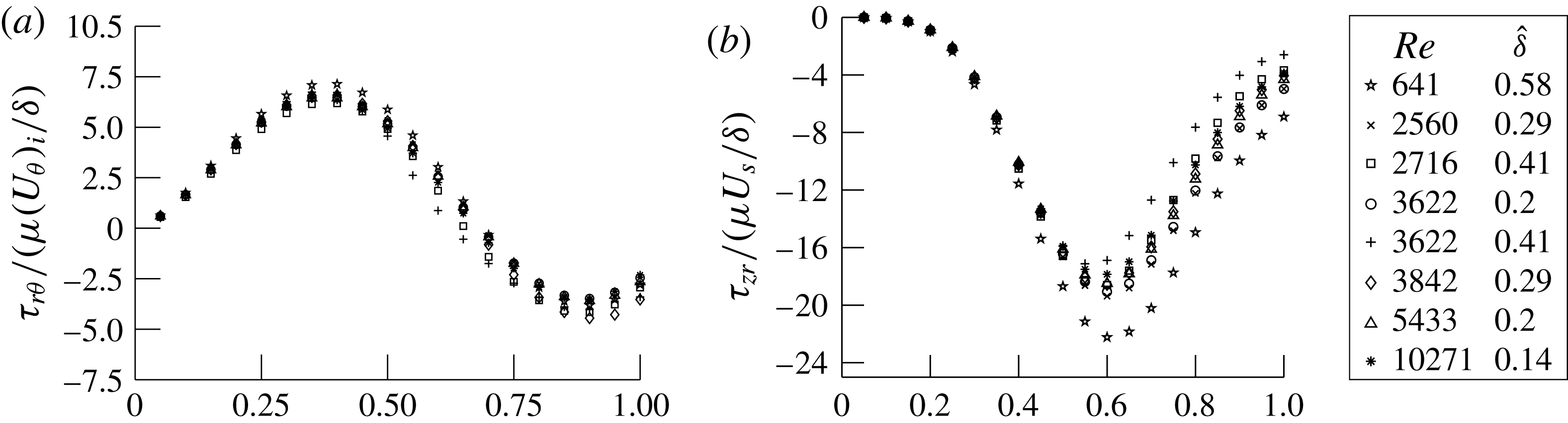
. Together, we observe large values of the WSS along the top (/bottom) and inner walls of the tube due to the secondary flows which have similar magnitude to the WSS due to axial flows. We also see large spatial and temporal variations in the WSS due to the combined effects of pulsatility and formation of the secondary flow structures arising out of curvature effects:
 $$\begin{eqnarray}\displaystyle & \displaystyle \unicode[STIX]{x1D70F}_{r\unicode[STIX]{x1D703}}\sim \unicode[STIX]{x1D707}\frac{(U_{\unicode[STIX]{x1D703}})_{i}}{\unicode[STIX]{x1D6FF}}, & \displaystyle\end{eqnarray}$$
 $$\begin{eqnarray}\displaystyle & \displaystyle \unicode[STIX]{x1D70F}_{zr}\sim \unicode[STIX]{x1D707}\frac{U_{s}}{\unicode[STIX]{x1D6FF}}. & \displaystyle\end{eqnarray}$$
The components (a)
 $\unicode[STIX]{x1D70F}_{r\unicode[STIX]{x1D703}}$
on the medial (
 $r{-}\unicode[STIX]{x1D703}$
) plane
 $(\hat{z}=0)$
at the P90 plane on the inner wall, normalized by
 $\unicode[STIX]{x1D707}(U_{\unicode[STIX]{x1D703}})_{i}/\unicode[STIX]{x1D6FF}$
, and (b)
 $\unicode[STIX]{x1D70F}_{zr}$
on
 $\hat{z}=\pm 1$
(top/bottom wall) at
 $(r-r_{i})/a=1$
, normalized by
 $\unicode[STIX]{x1D707}U_{s}/\unicode[STIX]{x1D6FF}$
, are plotted with the non-dimensional time for the different cases that were obtained from the numerical simulations.

Figures 19(a) and 19(b) show two different components of the WSS from the computations for the same eight cases as shown in figure 14 and plotted as a function of time. Figure 19(a) shows the axial component of the WSS on the inner wall at the medial plane at P90, normalized by the scale for
 $\unicode[STIX]{x1D70F}_{r\unicode[STIX]{x1D703}}$
, given by (4.8), where
 $(U_{\unicode[STIX]{x1D703}})_{i}$
is the axial velocity at the inner wall from the inviscid annular flow solution (A 15);
 $(U_{\unicode[STIX]{x1D703}})_{i}$
is calculated at
 $\hat{t}=0.5$
when the piston velocity is maximum, and
 $\unicode[STIX]{x1D6FF}$
is based on the time of the pulse,
 $T$
(see table 2). Figure 19(b) shows the transverse component of the WSS in the radial direction on the top (/bottom) wall, normalized by the scale for
 $\unicode[STIX]{x1D70F}_{zr}$
, given by (4.9). There is reasonable collapse of data for both of the WSS components. Cases that have higher
 $\hat{\unicode[STIX]{x1D6FF}}$
show larger deviations, especially at later times. The collapse suggests that the scales we have used to normalize the two WSS components (4.8) and (4.9) are appropriate and provide a useful measure for estimating the axial and transverse components of the WSS in curved pipes.
5 Discussion
Our study, covering a wide range of
 $De$
and
 $\unicode[STIX]{x1D6FC}$
numbers, shows the coupled roles of pulsatility and curvature on the creation of secondary flows and flow separation in a square cross-sectional tube with high curvature. Secondary flows, collision of flow structures in the medial plane and separations that are similar to those seen in our study also occur in circular cross-section tubes (Talbot & Gong Reference Talbot and Gong1983; Chang & Tarbell Reference Chang and Tarbell1985; Hamakiotes & Berger Reference Hamakiotes and Berger1988; Rindt et al.
Reference Rindt, Van Steenhoven, Janssen and Vossers1991; Komai & Tanishita Reference Komai and Tanishita1997; Boiron et al.
Reference Boiron, Deplano and Pelissier2007; Timité et al.
Reference Timité, Castelain and Peerhossaini2010). The advection of low-momentum boundary layer fluid by the secondary flow was also discussed earlier (Clarke & Denier Reference Clarke and Denier2009). The direct connection between flow separation and secondary flows that was shown in our work was, however, not discussed in these studies. Specifically, our studies show that the forcing due to the centrifugal force imbalance in the plane on the horizontal walls causes the secondary wall jet, which subsequently impinges on the inner wall and moves radially inwards after collision (figure 3). In particular, we show that flow separation on the inner wall is linked to the secondary flow and is not due to a spatial adverse pressure gradient as previously thought (Chandran & Yearwood Reference Chandran and Yearwood1981; Talbot & Gong Reference Talbot and Gong1983). A primary difference between the square and circular cross-sections is that in the latter the forcing term is present along the periphery until the medial plane. In contrast, it is present only on the straight (top and bottom) walls for square cross-sectional tubes. The scaling relations developed for the secondary flow (4.3) and WSS (4.8) and (4.9) for the square cross-section tube in our study will also apply to the circular cross-section case modified using equations suitable for a circular cross-section. The WSS distributions in the transverse plane will also have minor differences between circular and square cross-sections (figures 18
c and 18
d). Komai & Tanishita (Reference Komai and Tanishita1997) used a circular cross-sectional tube of high curvature (
 $\unicode[STIX]{x1D6FD}\sim 0.5$
) to show similar variations in the axial WSS direction over time to those seen in our study (figure 18
b). We note that the ratio of the maximum WSS on the inner to outer walls is approximately twice that in both of these cases. The wide parametric space covered in our study and the scaling relations permit us to quantify the observed spatio-temporal variations in the different components of the WSS which arise due to pulsatility and curvature (figures 18 and 19).
Variations in the shear stresses, radial pressures, circumferential and longitudinal stretching of the vessel wall during each cardiac cycle together influence the cell mechanobiological processes that are important in the progression of diseases like atherosclerosis, aneurysms and dissections (Humphery Reference Humphery2002; Babu, Byju & Gundiah Reference Babu, Byju and Gundiah2015). Endothelial cells, lining the arterial lumen, respond to changes in the magnitude and direction of the shear stress due to pulsatile blood flows (Topper & Gimbrone Jr Reference Topper and Gimbrone1999; Davies Reference Davies2009; Chiu & Chien Reference Chiu and Chien2011). The WSS is hypothesized to determine the spatio-temporal cellular changes to pulsatile forces (Ku et al.
Reference Ku, Giddens, Zarins and Glagov1985; Chien Reference Chien2008). Regions with low mean WSS, and those where shear stresses change in direction during the cycle, are reported to be preferential sites for atherosclerotic plaque formation (Ku Reference Ku1997; Chien Reference Chien2007; Wang et al.
Reference Wang, Baker, Chen and Schwartz2013). Studies on in vitro cultures of endothelial cells clearly show pro-inflammatory effects due to disturbed flows which correlate with the failure of cells in aligning and elongating along the flow direction (Davies Reference Davies1995; Passerini, Milsted & Rittgers Reference Passerini, Milsted and Rittgers2003; Chien Reference Chien2007; Berk Reference Berk2008). These inflammatory effects are, however, suppressed under high steady or pulsatile laminar flows. In the human aorta, flow separations on the inner arterial wall are hypothesized to be important in the formation of atherosclerosis (Chandran Reference Chandran1993; Davies Reference Davies2009). We show that the flow reversals and separations on the inner wall are intimately related to the secondary flow and are not due to a spatial pressure gradient in the axial flow direction. Further, the spatio-temporal variations of the WSS in the longitudinal and transverse directions may be estimated using (4.8) and (4.9) over a range of
 $De{-}\unicode[STIX]{x1D6FC}$
which occur in different vessels. The normalized WSS values in our study are similar to those quantified using patient-specific models obtained from CT and/or MR imaging (Morris et al.
Reference Morris, Delassus, Callanan, Walsh, Wallis, Grace and McGloughlin2005). Even though the motivation for this study was physiological flows in the ascending aorta, our results may be used for any pulse-like flow in a curved tube provided that the boundary layers are thin compared with the tube radius. In particular, the scaling relations developed in our study for secondary flows and WSS may also be used for tubes with different curvatures which are relevant in many physiological flows and in other engineering applications. Physiological flows occur in vessels with geometries that have varying non-circular cross-sections, branches, torsional twist, with elastic walls (Chandran Reference Chandran1993). We believe that the results from this study will enhance our understanding of secondary flows in such complex geometries.
6 Conclusions
We performed experimental flow visualization studies over a wide range of
 $De$
and
 $\unicode[STIX]{x1D6FC}$
of unsteady flow in a square cross-section tube of high curvature (
 $\unicode[STIX]{x1D6FD}=0.3$
). For the present study, we show that for unsteady flow in curved pipes, besides the classical non-dimensional Dean
 $(De)$
and Womersley
 $(\unicode[STIX]{x1D6FC})$
numbers, it is useful to recast these to get other parameters, namely
 $\hat{L}$
(the average distance the fluid moves in the axial direction over the time pulse period),
 $\hat{\unicode[STIX]{x1D6FF}}$
(the boundary layer thickness) and
 $Re_{\unicode[STIX]{x1D6FF}}$
(the Reynolds number based on the boundary layer thickness), which better explain some of the flow physics. The unsteady input flow was in the form of a single pulse. We performed numerical simulations for a few specific cases and obtained detailed quantitative information on the resulting flows. Secondary flows, having the structure of wall jets, form on the straight walls and move towards the inner wall. A subsequent collision of these wall jets on the inner wall leads to a re-entrant jet that moves radially inward towards the outer wall. During the deceleration phase, the low-momentum fluid in the jet reverses direction, and a separation zone is observed near the inner wall. The influence of secondary flow on flow separation is highlighted by a 2D simulation in a curved channel with the same boundary conditions where secondary flows are absent and negligible flow separation is observed. The secondary flow velocities are high,
 ${\sim}40\,\%$
of the peak piston velocity for case 2, and increase with
 $\hat{L}$
.
We show that the formation of the wall-jet-like secondary flow occurs due to an imbalance in the radial pressure gradient and centrifugal forces. We also derive scales for the secondary flow velocities (4.3) using the governing equations under the boundary layer assumption. In the limit of small curvature, the Reynolds number based on this secondary flow velocity scale becomes equal to the secondary streaming Reynolds number introduced by Lyne (Reference Lyne1971) for oscillatory flow in a loosely curved pipe. We also derived two additional scales using the secondary flow velocity scale. The first allows us to estimate the values of the transverse component of the WSS. The second scale is for
 $\hat{P}$
(4.6) and (4.7), which represents the displacement of fluid in the transverse plane due to the secondary flow and determines the final structures of the flow. Several studies have observed collision of vortical structures on the inner wall, but none have mathematically derived scales for
 $\hat{P}$
and the WSS.
The results from our study, performed in a square cross-section tube, may, however, explain many of the flow features reported in unsteady flows in circular cross-section tubes with high curvature. Moreover, the scales for the secondary flow velocity and WSS can be derived using an appropriate coordinate system for geometries with circular cross-sections as well.
Acknowledgements
We thank Mr A. Augusty for help with fabrication of the experimental set-up and preliminary experiments performed during the course of his Master’s project. We thank the reviewers for constructive comments which have improved the study conclusions. The computational facilities made available at Supercomputer Education and Research Center, Indian Institute of Science Bangalore are gratefully acknowledged. N.G. acknowledges financial support from the Department of Biotechnology (BT/PR13926/MED/31/97/2010) and the Department of Science and Technology – Ramanujan grant and fellowship (SR/S2/RJN – 42/2009).
Supplementary movies
Supplementary movies are available at https://doi.org/10.1017/jfm.2017.7.
Appendix A. Scaling analysis for secondary flow velocity
We consider the boundary layers on the top and bottom walls to develop the scaling for the secondary flow. All of the variables are non-dimensionalized as follows:
 $$\begin{eqnarray}\left.\begin{array}{@{}c@{}}\unicode[STIX]{x1D6FD}=a/R,\quad \hat{r}=r/a,\quad \bar{r}=r/R=\hat{r}\unicode[STIX]{x1D6FD},\quad \bar{z}=z/\unicode[STIX]{x1D6FF},\quad \hat{t}=t/T,\quad \hat{U} _{p}=U_{p}/U_{p(max)},\\ \bar{u}_{r}=u_{r}/U_{s},\quad \hat{u} _{\unicode[STIX]{x1D703}}=u_{\unicode[STIX]{x1D703}}/U_{p(max)},\quad \hat{u} _{\unicode[STIX]{x1D703}(\mathit{invis})}=u_{\unicode[STIX]{x1D703}(\mathit{invis})}/U_{p(max)},\quad \hat{u} _{z}=u_{z}/(u_{z})_{n},\end{array}\right\}\end{eqnarray}$$
where
 $(u_{z})_{n}$
is given by (A 4). Here,
 $\unicode[STIX]{x1D6FF}$
is the approximate boundary layer thickness at the end of the pulse and is given by
 $\unicode[STIX]{x1D6FF}\sim 3.7\sqrt{\unicode[STIX]{x1D708}T}$
.
The continuity equation is
 $$\begin{eqnarray}\frac{u_{r}}{r}+\frac{\unicode[STIX]{x2202}u_{r}}{\unicode[STIX]{x2202}r}+\frac{1}{r}\frac{\unicode[STIX]{x2202}u_{\unicode[STIX]{x1D703}}}{\unicode[STIX]{x2202}\unicode[STIX]{x1D703}}+\frac{\unicode[STIX]{x2202}u_{z}}{\unicode[STIX]{x2202}z}=0.\end{eqnarray}$$
Assuming the flow to be fully developed,
 $\unicode[STIX]{x2202}u_{\unicode[STIX]{x1D703}}/\unicode[STIX]{x2202}\unicode[STIX]{x1D703}=0$
, we get
 $$\begin{eqnarray}\frac{U_{s}}{R}\frac{\bar{u}_{r}}{\bar{r}}+\frac{U_{s}}{a}\frac{\unicode[STIX]{x2202}\bar{u}_{r}}{\unicode[STIX]{x2202}\hat{r}}+\frac{(u_{z})_{n}}{\unicode[STIX]{x1D6FF}}\frac{\unicode[STIX]{x2202}\hat{u} _{z}}{\unicode[STIX]{x2202}\bar{z}}=0.\end{eqnarray}$$
Because each coefficient in the above equation should be of the same order, the scale for
 $u_{z}$
is given by
 $$\begin{eqnarray}(u_{z})_{n}\sim \frac{U_{s}\unicode[STIX]{x1D6FF}}{a}.\end{eqnarray}$$
The Navier–Stokes equation in the
 $r$
-direction in cylindrical coordinates is
 $$\begin{eqnarray}\displaystyle & & \displaystyle \frac{\unicode[STIX]{x2202}u_{r}}{\unicode[STIX]{x2202}t}+u_{r}\frac{\unicode[STIX]{x2202}u_{r}}{\unicode[STIX]{x2202}r}+\frac{u_{\unicode[STIX]{x1D703}}}{r}\frac{\unicode[STIX]{x2202}u_{r}}{\unicode[STIX]{x2202}\unicode[STIX]{x1D703}}+u_{z}\frac{\unicode[STIX]{x2202}u_{r}}{\unicode[STIX]{x2202}z}-\frac{u_{\unicode[STIX]{x1D703}}^{2}}{r}\nonumber\\ \displaystyle & & \displaystyle \quad =-\frac{1}{\unicode[STIX]{x1D70C}}\frac{\unicode[STIX]{x2202}p}{\unicode[STIX]{x2202}r}+\unicode[STIX]{x1D708}\left(\frac{1}{r}\frac{\unicode[STIX]{x2202}u_{r}}{\unicode[STIX]{x2202}r}+\frac{\unicode[STIX]{x2202}^{2}u_{r}}{\unicode[STIX]{x2202}r^{2}}+\frac{1}{r^{2}}\frac{\unicode[STIX]{x2202}^{2}u_{r}}{\unicode[STIX]{x2202}\unicode[STIX]{x1D703}^{2}}+\frac{\unicode[STIX]{x2202}^{2}u_{r}}{\unicode[STIX]{x2202}z^{2}}-\frac{u_{r}}{r^{2}}-\frac{2}{r^{2}}\frac{\unicode[STIX]{x2202}u_{\unicode[STIX]{x1D703}}}{\unicode[STIX]{x2202}\unicode[STIX]{x1D703}}\right).\end{eqnarray}$$
In an inviscid annular flow, the
 $r$
and
 $z$
components of the velocity (
 $u_{r}$
,
 $u_{z}$
) are zero; hence (A 5) reduces to
 $$\begin{eqnarray}\frac{\unicode[STIX]{x2202}p}{\unicode[STIX]{x2202}r}=\frac{\unicode[STIX]{x1D70C}u_{\unicode[STIX]{x1D703}(\mathit{invis})}^{2}}{r}.\end{eqnarray}$$
This pressure gradient is imposed in the boundary layer. Substituting (A 6) into (A 5), the Navier–Stokes equation in the
 $r$
-direction in the boundary layer is given by
 $$\begin{eqnarray}\displaystyle & & \displaystyle \!\!\!\frac{\unicode[STIX]{x2202}u_{r}}{\unicode[STIX]{x2202}t}+u_{r}\frac{\unicode[STIX]{x2202}u_{r}}{\unicode[STIX]{x2202}r}+\frac{u_{\unicode[STIX]{x1D703}}}{r}\frac{\unicode[STIX]{x2202}u_{r}}{\unicode[STIX]{x2202}\unicode[STIX]{x1D703}}+u_{z}\frac{\unicode[STIX]{x2202}u_{r}}{\unicode[STIX]{x2202}z}\nonumber\\ \displaystyle & & \displaystyle \!\!\!\quad =-\left(\frac{u_{\unicode[STIX]{x1D703}(\mathit{invis})}^{2}}{r}-\frac{u_{\unicode[STIX]{x1D703}}^{2}}{r}\right)+\unicode[STIX]{x1D708}\left(\frac{1}{r}\frac{\unicode[STIX]{x2202}u_{r}}{\unicode[STIX]{x2202}r}+\frac{\unicode[STIX]{x2202}^{2}u_{r}}{\unicode[STIX]{x2202}r^{2}}+\frac{1}{r^{2}}\frac{\unicode[STIX]{x2202}^{2}u_{r}}{\unicode[STIX]{x2202}\unicode[STIX]{x1D703}^{2}}+\frac{\unicode[STIX]{x2202}^{2}u_{r}}{\unicode[STIX]{x2202}z^{2}}-\frac{u_{r}}{r^{2}}-\frac{2}{r^{2}}\frac{\unicode[STIX]{x2202}u_{\unicode[STIX]{x1D703}}}{\unicode[STIX]{x2202}\unicode[STIX]{x1D703}}\right).\qquad \quad\end{eqnarray}$$
The axial velocity in the boundary layer varies from 0 at the wall to the inviscid axial velocity at the edge of the boundary layer,
 $$\begin{eqnarray}u_{\unicode[STIX]{x1D703}}(r,z,t)=u_{\unicode[STIX]{x1D703}(\mathit{invis})}(r,t)f(z,t),\end{eqnarray}$$
where the function
 $f$
satisfies the boundary conditions
 $$\begin{eqnarray}f(z,t)=\left\{\begin{array}{@{}ll@{}}1,\quad & \text{at}~z=\pm (a-\unicode[STIX]{x1D6FF}),\\ 0,\quad & \text{at}~z=\pm a.\end{array}\right.\end{eqnarray}$$
Substituting (A 8) into (A 7),
 $$\begin{eqnarray}\displaystyle & & \displaystyle \frac{\unicode[STIX]{x2202}u_{r}}{\unicode[STIX]{x2202}t}+u_{r}\frac{\unicode[STIX]{x2202}u_{r}}{\unicode[STIX]{x2202}r}+\frac{u_{\unicode[STIX]{x1D703}}}{r}\frac{\unicode[STIX]{x2202}u_{r}}{\unicode[STIX]{x2202}\unicode[STIX]{x1D703}}+u_{z}\frac{\unicode[STIX]{x2202}u_{r}}{\unicode[STIX]{x2202}z}\nonumber\\ \displaystyle & & \displaystyle \quad =-\frac{u_{\unicode[STIX]{x1D703}(\mathit{invis})}^{2}}{r}\left(1-f^{2}(z,t)\right)+\unicode[STIX]{x1D708}\left(\frac{1}{r}\frac{\unicode[STIX]{x2202}u_{r}}{\unicode[STIX]{x2202}r}+\frac{\unicode[STIX]{x2202}^{2}u_{r}}{\unicode[STIX]{x2202}r^{2}}+\frac{1}{r^{2}}\frac{\unicode[STIX]{x2202}^{2}u_{r}}{\unicode[STIX]{x2202}\unicode[STIX]{x1D703}^{2}}+\frac{\unicode[STIX]{x2202}^{2}u_{r}}{\unicode[STIX]{x2202}z^{2}}-\frac{u_{r}}{r^{2}}-\frac{2}{r^{2}}\frac{\unicode[STIX]{x2202}u_{\unicode[STIX]{x1D703}}}{\unicode[STIX]{x2202}\unicode[STIX]{x1D703}}\right).\nonumber\\ \displaystyle & & \displaystyle\end{eqnarray}$$
Hence, (A 10) in non-dimensional form and in the fully developed flow assumption is
 $$\begin{eqnarray}\displaystyle \frac{\unicode[STIX]{x2202}\bar{u}_{r}}{\unicode[STIX]{x2202}\hat{t}}+\left(\frac{U_{s}T}{a}\right)\bar{u}_{r}\frac{\unicode[STIX]{x2202}\bar{u}_{r}}{\unicode[STIX]{x2202}\hat{r}}+\left(\frac{U_{s}T}{a}\right)\bar{u}_{z}\frac{\unicode[STIX]{x2202}\bar{u}_{r}}{\unicode[STIX]{x2202}\bar{z}} & = & \displaystyle -\frac{T}{U_{s}}\frac{U_{p(max)}^{2}\hat{u} _{\unicode[STIX]{x1D703}(\mathit{invis})}^{2}}{\bar{r}R}(1-f^{2}(z,t))\nonumber\\ \displaystyle & & \displaystyle +\,\frac{\unicode[STIX]{x1D708}T}{\unicode[STIX]{x1D6FF}^{2}}\left(\frac{\unicode[STIX]{x1D6FF}^{2}}{aR\bar{r}}\frac{\unicode[STIX]{x2202}\bar{u}_{r}}{\unicode[STIX]{x2202}\hat{r}}+\frac{\unicode[STIX]{x1D6FF}^{2}}{a^{2}}\frac{\unicode[STIX]{x2202}^{2}\bar{u}_{r}}{\unicode[STIX]{x2202}\hat{r}^{2}}+\frac{\unicode[STIX]{x2202}^{2}\bar{u}_{r}}{\unicode[STIX]{x2202}\bar{z}^{2}}-\frac{\unicode[STIX]{x1D6FF}^{2}}{a^{2}}\frac{\bar{u}_{r}}{\hat{r}^{2}}\right).\nonumber\\ \displaystyle & & \displaystyle\end{eqnarray}$$
Assuming
 $\unicode[STIX]{x1D6FF}^{2}/a^{2}$
,
 $(\unicode[STIX]{x1D6FF}^{2}/aR)\ll 1$
, we get
 $$\begin{eqnarray}\displaystyle \frac{\unicode[STIX]{x2202}\bar{u}_{r}}{\unicode[STIX]{x2202}\hat{t}}+\left(\frac{U_{s}T}{a}\right)\bar{u}_{r}\frac{\unicode[STIX]{x2202}\bar{u}_{r}}{\unicode[STIX]{x2202}\hat{r}}+\left(\frac{U_{s}T}{a}\right)\hat{u} _{z}\frac{\unicode[STIX]{x2202}\bar{u}_{r}}{\unicode[STIX]{x2202}\bar{z}} & = & \displaystyle -\frac{T}{U_{s}}\frac{U_{p(max)}^{2}\hat{u} _{\unicode[STIX]{x1D703}(\mathit{invis})}^{2}}{\bar{r}R}(1-f^{2}(z,t))\nonumber\\ \displaystyle & & \displaystyle +\,\frac{\unicode[STIX]{x1D708}T}{\unicode[STIX]{x1D6FF}^{2}}\left(\frac{\unicode[STIX]{x2202}^{2}\bar{u}_{r}}{\unicode[STIX]{x2202}\bar{z}^{2}}\right).\end{eqnarray}$$
We assume the velocity distribution in the inviscid core to be same as in the potential annular flow with a circulation of
 $2\unicode[STIX]{x03C0}\unicode[STIX]{x1D6E4}$
,
 $$\begin{eqnarray}u_{\unicode[STIX]{x1D703}(\mathit{invis})}(r,t)=\frac{\unicode[STIX]{x1D6E4}(t)}{r}.\end{eqnarray}$$
Using mass balance between the inlet of the pipe and the fully developed curved region,
 $$\begin{eqnarray}\int _{R-a}^{R+a}u_{\unicode[STIX]{x1D703}(\mathit{invis})}(r,t)\,\text{d}r=U_{p}(t)(2a).\end{eqnarray}$$
Thus,
 $$\begin{eqnarray}u_{\unicode[STIX]{x1D703}(\mathit{invis})}(r,t)=\frac{U_{p}(t)(2a)}{r}\unicode[STIX]{x1D705}\end{eqnarray}$$
or
 $$\begin{eqnarray}\hat{u} _{\unicode[STIX]{x1D703}(\mathit{invis})}(r,t)=\frac{u_{\unicode[STIX]{x1D703}(\mathit{invis})}(r,t)}{U_{p(max)}}=2\hat{U} _{p}\left(\frac{1}{\bar{r}}\right)\unicode[STIX]{x1D6FD}\unicode[STIX]{x1D705},\end{eqnarray}$$
where
 $$\begin{eqnarray}\unicode[STIX]{x1D705}=1/\ln \left(\frac{R+a}{R-a}\right)=1/\ln \left(\frac{1+\unicode[STIX]{x1D6FD}}{1-\unicode[STIX]{x1D6FD}}\right).\end{eqnarray}$$
Substituting (A 16) into (A 12),
 $$\begin{eqnarray}\displaystyle \frac{\unicode[STIX]{x2202}\bar{u}_{r}}{\unicode[STIX]{x2202}\hat{t}}+\left(\frac{U_{s}T}{a}\right)\left(\bar{u}_{r}\frac{\unicode[STIX]{x2202}\bar{u}_{r}}{\unicode[STIX]{x2202}\hat{r}}+\hat{u} _{z}\frac{\unicode[STIX]{x2202}\bar{u}_{r}}{\unicode[STIX]{x2202}\bar{z}}\right) & = & \displaystyle -\left(4\frac{U_{p(max)}^{2}T}{RU_{s}}\unicode[STIX]{x1D6FD}^{2}\unicode[STIX]{x1D705}^{2}\right)\frac{\hat{U} _{p}^{2}\left(1-f^{2}(z,t)\right)}{\bar{r}^{3}}\nonumber\\ \displaystyle & & \displaystyle +\,\frac{\unicode[STIX]{x1D708}T}{\unicode[STIX]{x1D6FF}^{2}}\left(\frac{\unicode[STIX]{x2202}^{2}\bar{u}_{r}}{\unicode[STIX]{x2202}\bar{z}^{2}}\right).\end{eqnarray}$$
To get the scale of the secondary flow
 $U_{s}$
, we show that each of the terms in the above equation is of
 $O(1)$
. On the left-hand side, the first term is of
 $O(1)$
and the coefficient of the second term is
 $=P/a=2\hat{P}$
, which represents the distance traversed by the secondary flow front. From figure 16, this term is either lower order, which means that the convective terms are negligible, or of
 $O(1)$
for most of the cases in the current study. On the right-hand side, the coefficient of the second term is of
 $O(1)$
, because
 $\unicode[STIX]{x1D6FF}\sim \sqrt{\unicode[STIX]{x1D708}T}$
. Hence, the scale for the secondary flow velocity is given by
 $$\begin{eqnarray}U_{s}=4c\frac{U_{p(max)}^{2}T}{R}\unicode[STIX]{x1D6FD}^{2}\unicode[STIX]{x1D705}^{2}.\end{eqnarray}$$
We choose
 $c=1/(4\unicode[STIX]{x03C0})$
, so that in the limit
 $\unicode[STIX]{x1D6FD}\rightarrow 0$
,
 $U_{s}$
reduces to the secondary flow velocity scale introduced by Lyne (Reference Lyne1971),
 $$\begin{eqnarray}U_{s}=\frac{1}{\unicode[STIX]{x03C0}}\frac{U_{p(max)}^{2}T}{R}\unicode[STIX]{x1D6FD}^{2}\unicode[STIX]{x1D705}^{2},\end{eqnarray}$$
or, in terms of
 $Re_{\unicode[STIX]{x1D6FF}}$
,
 $\hat{\unicode[STIX]{x1D6FF}}$
and in terms of
 $Re$
,
 $\hat{\unicode[STIX]{x1D6FF}}$
,
 $$\begin{eqnarray}\hat{U} _{s}=\frac{U_{s}}{U_{p(max)}}\sim \frac{1}{13.69\unicode[STIX]{x03C0}}Re_{\unicode[STIX]{x1D6FF}}\hat{\unicode[STIX]{x1D6FF}}\unicode[STIX]{x1D6FD}^{3}\unicode[STIX]{x1D705}^{2}\sim \frac{1}{27.38\unicode[STIX]{x03C0}}Re\hat{\unicode[STIX]{x1D6FF}}^{2}\unicode[STIX]{x1D6FD}^{3}\unicode[STIX]{x1D705}^{2}.\end{eqnarray}$$
It should be noted that the scale for
 $U_{s}$
does not hold when
 $2\hat{P}$
is higher than
 $O(1)$
or when the boundary layer assumption is not valid.
Appendix B. Scaling relations for
 $\hat{L}$
and
$\hat{P}$


The term
 $L$
is the average distance travelled by the fluid in the axial direction during
 $T$
. Thus,
 $$\begin{eqnarray}\hat{L}=\frac{L}{2a}=\frac{\displaystyle \int _{0}^{T}U_{p}(t)\,\text{d}t}{2a}=\frac{U_{p(max)}T}{4a}.\end{eqnarray}$$
Using
 $\unicode[STIX]{x1D6FF}=3.7\sqrt{\unicode[STIX]{x1D708}T}$
, we have
 $$\begin{eqnarray}\hat{L}\sim 1.8\times 10^{-2}Re_{\unicode[STIX]{x1D6FF}}\hat{\unicode[STIX]{x1D6FF}}.\end{eqnarray}$$
Similarly, the distance traversed by the fluid particle in the transverse
 $(r{-}z)$
plane is given by
 $$\begin{eqnarray}\hat{P}=\frac{P}{2a}=\frac{\displaystyle \int _{0}^{T}u_{s}(t)\,\text{d}t}{2a}\sim \frac{U_{s}T}{2a}.\end{eqnarray}$$
Substituting the scale for
 $U_{s}$
, from (A 19),
 $$\begin{eqnarray}\hat{P}\sim \frac{1}{\unicode[STIX]{x03C0}}\frac{U_{p(max)}^{2}T}{R}\unicode[STIX]{x1D6FD}^{2}\unicode[STIX]{x1D705}^{2}\frac{T}{2a}.\end{eqnarray}$$
Using
 $L=U_{p(max)}T/2$
, equation (B 4) is given by
 $$\begin{eqnarray}\hat{P}\sim \frac{8}{\unicode[STIX]{x03C0}}\hat{L}^{2}\unicode[STIX]{x1D6FD}^{3}\unicode[STIX]{x1D705}^{2},\end{eqnarray}$$
or, in terms of
 $Re_{\unicode[STIX]{x1D6FF}}$
and
 $\hat{\unicode[STIX]{x1D6FF}}$
, by using (B 2),
 $$\begin{eqnarray}\hat{P}\sim 8.5\times 10^{-4}Re_{\unicode[STIX]{x1D6FF}}^{2}\hat{\unicode[STIX]{x1D6FF}}^{2}\unicode[STIX]{x1D6FD}^{3}\unicode[STIX]{x1D705}^{2}.\end{eqnarray}$$