2. Basic equations

Consider a fully ionized two-fluid non-relativistic plasma. In the hydrodynamic approximation that takes into account its main dissipations, the plasma dynamics is described by the Braginskii equations (Braginskii Reference Braginskii and Leontovich1965)

where ${\it\rho}_{\pm }=m_{\pm }n_{\pm }$ , $m_{{\it\Sigma}}=m_{+}+m_{-}$ , and the subscripts $\pm$ refer to electrons and ions. For the dissipative terms ${\it\bf\Pi}_{\pm }$ , $\boldsymbol{R}_{\pm }$ , $\boldsymbol{q}_{\pm }$ , $Q_{\pm }$ we adopt the following commonly used simplified expressions:

1. (i) $\unicode[STIX]{x1D63F}_{\pm }=\text{def}\,\boldsymbol{v}_{\pm }=\Vert \unicode[STIX]{x1D63F}_{{\it\alpha}{\it\beta}}^{\pm }\Vert ,\unicode[STIX]{x1D63F}_{{\it\alpha}{\it\beta}}^{\pm }=((\partial v_{\pm }^{{\it\alpha}})/(\partial x_{{\it\beta}})+(\partial v_{\pm }^{{\it\beta}})/(\partial x_{{\it\alpha}}))/2$ is the deformation tensor,

2. (ii) ${\it\bf\Pi}_{\pm }=2{\it\mu}_{\pm }\unicode[STIX]{x1D63F}_{\pm }+({\it\nu}_{\pm }-{\textstyle \frac{2}{3}}{\it\mu}_{\pm })\text{tr}\,\unicode[STIX]{x1D63F}_{\pm }\unicode[STIX]{x1D644}_{3}$  is the viscous stress tensor,

3. (iii) $\boldsymbol{R}_{\pm }=\pm ((e_{+}e_{-}n_{+}n_{-})/{\it\sigma})(\boldsymbol{v}_{+}-\boldsymbol{v}_{-})$ is the body force of friction between the components,

4. (iv) $Q_{\pm }=\pm b(T_{-}-T_{+})$ is the heat exchanged by the plasma components in elastic collisions,

5. (v) $\boldsymbol{q}_{\pm }=-{\it\eta}_{\pm }\boldsymbol{{\rm\nabla}}T_{\pm }$ is Fourier’s law for the heat flow in each plasma component.

The hydrodynamic viscosities of electrons and ions ${\it\mu}_{\pm }$ , ${\it\nu}_{\pm }$ are functions of $T_{+}$ , $T_{-}$ ; the plasma conductivity ${\it\sigma}$ and the coefficient of heat transfer $b$ are functions of the electron temperature $T_{-}$ . The approach described below can be easily generalized to more complex expressions for ${\it\bf\Pi}_{\pm }$ , $\boldsymbol{R}_{\pm }$ , $\boldsymbol{q}_{\pm }$ , $Q_{\pm }$ taking into account the thermal force and the anisotropy of magnetized plasma (Spitzer Reference Spitzer1962; Braginskii Reference Braginskii and Leontovich1965).

The system (2.1) is closed by Maxwell’s equations for the quasi-stationary magnetic field:

combined with the expressions for the transport coefficients ${\it\mu}_{\pm }$ , ${\it\nu}_{\pm }$ , ${\it\sigma}$ , $b$ , ${\it\eta}_{\pm }$ taken from Spitzer (Reference Spitzer1962), Braginskii (Reference Braginskii and Leontovich1965). Below, we need only the expressions for ${\it\mu}_{\pm }$ , ${\it\sigma}$ :

where $m_{i}=m_{+}$ , $m_{e}=m_{-}$ , $e=e_{-}$ is the electron charge, $Z$ is the multiplicity of the ion charge ( $e_{+}=Ze$ ), $L$ is the Coulomb logarithm (below, we take $L=15$ ), ${\it\rho}={\it\rho}_{+}+{\it\rho}_{-}$ , and the temperatures $T_{\pm }$ are measured in ergs. The formulae for the transport coefficients are theoretical and are refined from time to time. Thus, a significant reduction in electron viscosity is justified in Bobrova, Lazzaro & Sasorov (Reference Bobrova, Lazzaro and Sasorov2005).

3. Equations of electromagnetic hydrodynamics (EMHD) for plasma

At first sight, system (2.1) and (2.2) contains no equation for the electric field  $\boldsymbol{E}$ . However, such an equation can be easily obtained, if one takes into account the relations between some unknown functions in (2.1) and (2.2): namely, the velocities $\boldsymbol{v}_{+}$ , $\boldsymbol{v}_{-}$ are related by Ampere’s law, and the densities ${\it\rho}_{+}$ , ${\it\rho}_{-}$ are related by the condition of quasi-neutrality. Excluding the corresponding unknown variables, we come to a one-fluid form of system (2.1) and (2.2) with an equation for $\boldsymbol{E}$ . In problems of plasma statics, it is convenient to take $\boldsymbol{v}_{+}$ , ${\it\rho}_{+}$ as independent variables, while in problems of electron hydrodynamics, it is preferable to take $\boldsymbol{v}_{-}$ , ${\it\rho}_{-}$ . In the general case, we choose mass velocity $\boldsymbol{U}=({\it\rho}_{+}\boldsymbol{v}_{+}+{\it\rho}_{-}\boldsymbol{v}_{-})/{\it\rho}$ and the summed plasma density ${\it\rho}={\it\rho}_{+}+{\it\rho}_{-}$ as independent unknown variables. Then $\boldsymbol{v}_{\pm }$ , ${\it\rho}_{\pm }$ are expressed through ${\it\rho}$ , $\boldsymbol{U}$ by the simple formulae:

Passing to the variables ${\it\rho}$ , $\boldsymbol{U}$ in system (2.1) and (2.2), we obtain a mathematically equivalent system of electromagnetic hydrodynamics (EMHD) in divergent form:

where the momentum flux density tensor ${\it\bf\Pi}$ , the viscous stress tensor $\unicode[STIX]{x1D64B}$ and the tensor of ‘Hall terms’ $\unicode[STIX]{x1D652}$ are the following:

Finally, the tensors ${\it\bf\Pi}^{c}$ , ${\it\bf\Pi}_{\ast }^{c}$ , ${\it\bf\Pi}^{U}$ , ${\it\bf\Pi}_{\ast }^{U}$ have the form:

where $\unicode[STIX]{x1D63F}^{U}=\text{def}\,\boldsymbol{U}$ , $\unicode[STIX]{x1D63F}^{c}=\text{def}(\,\boldsymbol{j}/{\it\rho})$ are the strain tensor, $p_{{\it\Sigma}}=p_{+}+p_{-}$ , ${\it\mu}_{{\it\Sigma}}={\it\mu}_{+}+{\it\mu}_{-}$ , ${\it\nu}_{{\it\Sigma}}={\it\nu}_{+}+{\it\nu}_{-}$ , ${\it\mu}_{\ast }={\it\chi}_{-}{\it\mu}_{+}-{\it\chi}_{+}{\it\mu}_{-}$ , ${\it\nu}_{\ast }={\it\chi}_{-}{\it\nu}_{+}-{\it\chi}_{+}{\it\nu}_{-}$ , ${\it\mu}^{\ast }={\it\chi}_{-}^{2}{\it\mu}_{+}+{\it\chi}_{+}^{2}{\it\mu}_{-}$ , ${\it\nu}^{\ast }={\it\chi}_{-}^{2}{\it\nu}_{+}+{\it\chi}_{+}^{2}{\it\nu}_{-}$ .

Thus, system (3.2)–(3.4) is mathematically equivalent to (2.1) and (2.2). It is a one-fluid system that fully takes into account (in a symmetrical way) the inertia of electrons and ions. The equation for $\boldsymbol{E}$ coincides with the generalized Ohm’s law.

Finally, in the general case, the law of conservation of total energy holds for the solution of the EMHD equations:

where ${\it\varepsilon}=({\it\chi}_{+}{\it\varepsilon}_{+}+{\it\chi}_{-}{\it\varepsilon}_{-})/{\it\chi}$ is the bulk density of the plasma internal energy,

4. Dynamic equations of incompressible plasma

The quasi-neutral flow of an incompressible viscous electrically conducting fully ionized two-component electron–ion plasma, with the inertia of electrons fully taken into account by way of (3.2)–(3.4), is described by the following system of equations:

After the exclusion of $\boldsymbol{j}$ , the unknown quantities in (4.1) are $\boldsymbol{U}$ , $\boldsymbol{E}$ , $\boldsymbol{H}$ , $p_{\pm }$ . Thus, we have 11 scalar equations for 11 scalar functions. Note that (4.1) contains the additional equation $\text{div}\,\boldsymbol{E}=0$ , which is absent in (3.2)–(3.4). This allows us, on the one hand, to satisfy the condition of quasi-neutrality, and on the other, to make (4.1) a determined system.

Moreover, in the case of incompressible plasma, the expressions (3.4) for the viscous stress tensor are simplified to

Below we examine the stationary flow of incompressible plasma, for which (4.1) with $\partial /\partial t=0$ yields the following system of equations:

where tensors ${\it\bf\Pi}$ , $\unicode[STIX]{x1D64B}$ , $\unicode[STIX]{x1D652}$ are defined by (3.3). After excluding $\boldsymbol{j}$ and $\boldsymbol{E}$ from (4.3) we have a system of nine scalar equations for eight scalar functions, i.e. the components of the vector fields $\boldsymbol{H}$ , $\boldsymbol{U}$ and pressure $p_{+}$ , $p_{-}$ . However, in many practically important cases, the overdetermined system (4.3) can have physically interesting non-trivial solutions.

Strictly speaking, (4.1) is a non-closed system, since the viscosities ${\it\mu}_{\pm }$ and the hydrodynamic plasma conductivity ${\it\sigma}$ depend on temperature $T_{\pm }$ , as follows from (2.3). Following Landau & Lifshitz (Reference Landau and Lifshitz1987), in order to obtain a closed system, we supplement (4.1) with the equation for the temperatures:

where $c_{p}=T\partial S/\partial T$ is the specific heat at constant pressure. Thus, taking into account (3.1) and passing to the variables ${\it\rho}$ , $\boldsymbol{U}$ in (4.4), we obtain the closed system (4.1), (4.4). However, in what follows, ${\it\sigma}$ , ${\it\mu}_{\pm }$ (and therefore, $T_{\pm }$ ) are assumed to be constant. Thus, it is assumed that the Joule heating, as well as temperature variations of electrons and ions due to the work forces of viscous stresses, are negligibly small.

5. Steady flow in a planar channel

Consider a steady flow of incompressible plasma in an unlimited planar channel whose walls are parallel to the plane $Oyz$ and are defined by the equations $x=\pm \ell$ . First, we restrict ourselves to studying flows with plane symmetry ( $\partial /\partial y=\partial /\partial z=0$ ) caused by a constant pressure drop along the axis $z$ , i.e. we consider solutions of system (4.3) that have the form

and satisfy the boundary conditions

In particular, the channel walls are assumed to be fixed. More general boundary conditions are considered in § 9. From (4.3), it follows that $U_{x}=0$ , $j_{x}=0$ , $H_{x}=H_{0}$ . It is easy to show that $\partial p_{\pm }/\partial z=A_{\pm }=\text{const.}$ and $p_{\pm }(x,z)=A_{\pm }z+{\it\varphi}_{\pm }(x)$ , where the constants $A_{\pm }$ are given and the functions ${\it\varphi}_{\pm }(x)$ are to be found. It follows from (4.3) that $\boldsymbol{E}(x)\equiv \text{const.}$ , with $E_{x}$ given and $E_{y}$ , $E_{z}$ to be found from (4.3). To find the unknown quantities $H_{y}$ , $H_{z}$ , $U_{y}$ , $U_{z}$ , we substitute these functions into the equations $\text{Div}\,{\it\bf\Pi}=\text{Div}\unicode[STIX]{x1D64B}$ , $\text{rot}\,\boldsymbol{E}=0$ in (4.3) and obtain the following system of ordinary differential equations:

where $L(\unicode[STIX]{x1D63F})=[L_{ij}(\unicode[STIX]{x1D63F})]_{1\leqslant i,j\leqslant 4}$ , $L_{ij}(\unicode[STIX]{x1D63F})$ are algebraic polynomials of degree not greater than 4. The operator matrix $L(\unicode[STIX]{x1D63F})$ can be written in explicit form:

where ${\it\alpha}=H_{0}/4{\rm\pi}$ , ${\it\beta}=c{\it\mu}_{\ast }/(4{\rm\pi}{\it\rho})$ . Reducing system (5.3) to the canonical form, we obtain a $14\text{th}$ -order linear differential equations with constant real coefficients. The high order of the canonical system is a great obstacle to its integration. Therefore, we use the following artificial approach, assuming that $H_{0}({\it\mu}_{+}-{\it\mu}_{-})\neq 0$ (non-degenerate case).

6. Complexification of the system of equations

Let us identify the real plane with the complex plane: $a+\text{i}b=(a,b)$ , the multiplication of complex numbers being associated with the matrix–vector multiplication by the well-known formula

We see that the ( $4\times 4$ )-matrix operator $L(\unicode[STIX]{x1D63F})$ in (5.4) is divided into four ( $2\times 2$ )-blocks, each block being a matrix of the same type as in (6.1). Therefore, identifying the transverse plane $Oyz$ with the complex plane ( $x+\text{i}z=(y,z)$ , $H_{{\it\tau}}=H_{y}+\text{i}H_{z}$ , $U_{{\it\tau}}=U_{y}+\text{i}U_{z}$ ) and passing to the variables $w=\unicode[STIX]{x1D63F}H_{{\it\tau}}$ , $u=\unicode[STIX]{x1D63F}U_{{\it\tau}}$ , we reduce the system (5.3) to the form

Rewriting this system in scalar form,

expressing $u^{\prime }$ through $w$ from (6.3a ), and substituting the result into (6.3b ), we obtain the following explicit expression for $u$ in terms $w$ :

Substituting this expression into (6.3a ), we obtain the linear inhomogeneous differential equation of order four with respect to $w$ :

Since the characteristic polynomial of (6.5) is biquadratic, the squares of its roots ${\it\lambda}_{\pm }^{2}$ coincide with the zeros of the quadratic equation

and these zeros cannot be real, in view of non-degeneracy conditions $H_{0}({\it\mu}_{+}-{\it\mu}_{-})\neq 0$ . The general solution of (6.5) has the form

where $C_{i}$ , $1\leqslant i\leqslant 4$ , are arbitrary complex constants. Therefore, the general solution of (5.3), in complex notation, is written as

where $C_{i}$ , $R_{j}$ , $1\leqslant i\leqslant 4$ , $1\leqslant j\leqslant 2$ , are arbitrary complex constants. The complexification of the boundary conditions (5.2) gives

The six complex constants $C_{i}$ , $1\leqslant i\leqslant 4$ , $R_{j}$ , $1\leqslant j\leqslant 2$ , are uniquely determined from the six conditions in (6.9), and we obtain the following final expression for $H_{{\it\tau}}$ , $U_{{\it\tau}}$ :

The $x$ -component of the momentum equation (4.3), combined with the relation $j_{x}=0$ , allows us to calculate the function ${\it\varphi}_{\pm }(x)$ , and hence the pressure $p_{\pm }$ up to a constant:

Formulae (6.10) and (6.11) yield a complete mathematical solution to the problem of steady flow of an incompressible plasma in a planar channel with the boundary conditions (5.2).

Now, using (6.10), we can calculate the following secondary quantities:

1. (a) the average speed over the cross-section of the channel

   (6.12) $$\begin{eqnarray}\left\langle U_{{\it\tau}}\right\rangle =\frac{1}{2\ell }\int _{-\ell }^{\ell }U_{{\it\tau}}\,\text{d}x=\frac{\text{i}}{{\it\mu}_{{\it\Sigma}}}\frac{\partial p_{{\it\Sigma}}}{\partial z}\frac{({\it\kappa}_{-}-1)({\it\kappa}_{+}-1)}{{\it\kappa}_{-}-{\it\kappa}_{+}}\left(\frac{1}{{\it\lambda}_{+}^{2}}-\frac{1}{{\it\lambda}_{-}^{2}}\right);\end{eqnarray}$$

2. (b) the transverse electric field

   (6.13) $$\begin{eqnarray}E_{{\it\tau}}=E_{y}+\text{i}E_{z}=-\frac{c{\it\mu}_{+}{\it\mu}_{-}{\it\chi}^{2}}{{\it\mu}_{{\it\Sigma}}H_{0}{\it\rho}^{2}}A\frac{\partial p_{{\it\Sigma}}}{\partial z}+\frac{\text{i}{\it\chi}}{{\it\mu}_{{\it\Sigma}}{\it\rho}}\frac{\partial }{\partial z}({\it\mu}_{-}p_{+}-{\it\mu}_{+}p_{-})+\frac{\text{i}H_{0}}{c}\left\langle U_{{\it\tau}}\right\rangle ,\end{eqnarray}$$
   where $A=[{\it\lambda}_{+}^{2}{\it\kappa}_{+}({\it\kappa}_{-}-1)-{\it\lambda}_{-}^{2}{\it\kappa}_{-}({\it\kappa}_{+}-1)]/({\it\kappa}_{-}-{\it\kappa}_{+})$ ;

3. (c) forces of friction between the channel walls $x=\pm \ell$ and ions/electrons per unit area

   (6.14) $$\begin{eqnarray}F^{\pm }=-\frac{\text{i}\ell {\it\mu}_{\pm }}{{\it\mu}_{{\it\Sigma}}}\frac{\partial p_{{\it\Sigma}}}{\partial z}\left[1\mp \frac{\text{i}c{\it\chi}{\it\mu}_{\mp }}{H_{0}{\it\rho}}A\right].\end{eqnarray}$$

In particular, the total friction force on the wall of the plasma coincides with the expression $F=F^{+}+F_{-}=-\text{i}\ell \partial p_{{\it\Sigma}}/\partial z$ known in hydrodynamics (Landau & Lifshitz Reference Landau and Lifshitz1987). Note that $\left\langle \,j_{{\it\tau}}\right\rangle =0$ , $\left\langle v_{{\it\tau}}^{\pm }\right\rangle =\left\langle U_{{\it\tau}}\right\rangle$ .

7. Qualitative behaviour of the flow and the determining parameters

In the MHD approximation, the steady flow of incompressible plasma in a planar channel is described by the Hartmann formula (Kulikovskiy & Lyubimov Reference Kulikovskiy and Lyubimov1965) (see (7.7)). The result is quite different if one has to take into account the two-fluid structure of the plasma. It follows from (6.10) that for ${\it\lambda}_{\pm }=R_{\pm }+\text{i}{\it\omega}_{\pm }$ , $R_{\pm }>0$ , the longitudinal velocity $U_{{\it\tau}}$ is a superposition of harmonic oscillations with frequencies ${\it\omega}_{\pm }$ modulated in amplitude by the functions $\cosh R_{\pm }x$ , $\sinh R_{\pm }x$ . Moreover, (6.10) implies that the velocity profile $U_{{\it\tau}}$ has a spatial structure and does not belong to a single plane, as is the case of the Hartmann flow in the MHD theory.

To obtain the MHD and other limit cases, we introduce two dimensionless parameters:

Equation (7.1a ) is known as the Hartmann number (Kulikovskiy & Lyubimov Reference Kulikovskiy and Lyubimov1965), (7.1b ) is a new determining parameter containing the plasma density. From the characteristic equation for (6.5), it follows that

where $\sqrt{z}$ is the main branch of the root and ${\it\Lambda}_{\ast }=({\it\mu}_{+}{\it\mu}_{-})^{1/2}/{\it\mu}_{{\it\Sigma}}$ , ${\it\Lambda}_{0}=({\it\mu}_{-}-{\it\mu}_{+})/{\it\mu}_{{\it\Sigma}}$ . Below, it is assumed that ${\it\Lambda}_{0}<0$ (isothermal plasma). Now it is easy to write explicit expressions for $U_{{\it\tau}}$ , $H_{{\it\tau}}$ in terms of the parameters $\mathit{Ha}$ and ${\it\Gamma}$ , which completely determine the behaviour of the solution (6.10), (6.11). Thus, for $U_{{\it\tau}}$ and $\left\langle U_{{\it\tau}}\right\rangle$ , using (6.10), (6.12) we obtain the expressions

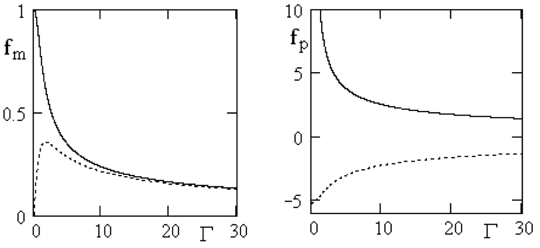
The numerically obtained graphs of the frequencies ${\it\omega}_{\pm }({\it\Gamma})$ and the amplitude modulation parameters $R_{\pm }({\it\Gamma})$ (in the units $\mathit{Ha}/\ell$ ) for deuterium plasma are given in figure 1. The asymptotics at zero and at infinity are easily obtained from the expansions into series of the functions $f_{\pm }({\it\Gamma})$ at the points ${\it\Gamma}=0$ and ${\it\Gamma}=\infty$ . For ${\it\Gamma}\rightarrow \infty$ , we have

For ${\it\Gamma}\rightarrow 0$ , we obtain

Figure 1.

Frequencies ${\it\omega}_{\pm }({\it\Gamma})$ ( $\cdots \cdots$ ); amplitude modulation parameters $R_{\pm }({\it\Gamma})$ (——).

The explicit dependence on the determining parameters allows us to pass to the limit in various physically important cases: the MHD limit ( ${\it\Gamma}\rightarrow 0$ , $\mathit{Ha}=\text{const.}$ ); the weak magnetic field limit ( ${\it\Gamma}\rightarrow 0$ , $\mathit{Ha}\rightarrow 0$ , ${\it\Gamma}/\mathit{Ha}=\text{const.}$ ); the strong magnetic field limit ( ${\it\Gamma},\mathit{Ha}\rightarrow +\infty$ , ${\it\Gamma}/\mathit{Ha}=\text{const.}$ ); the narrow channel limit ( $\mathit{Ha}\rightarrow 0$ , ${\it\Gamma}=\text{const.}$ ); the perfectly conducting plasma limit ( ${\it\Gamma},\mathit{Ha}\rightarrow +\infty$ , ${\it\Gamma}/\mathit{Ha}^{2}=\text{const.}$ ), etc. Especially important is the MHD limit, in which case ${\it\Gamma}\rightarrow 0$ :

Therefore $f_{+}({\it\Gamma})\rightarrow \infty$ , $f_{-}({\it\Gamma})\rightarrow 1$ , ${\it\kappa}_{+}\rightarrow 0$ , ${\it\kappa}_{-}\rightarrow \tanh \mathit{Ha}/\mathit{Ha}$ , $g_{+}\rightarrow 0$ , $g_{-}\rightarrow 1$ . Taking into account the above relations, we see that the expression (7.3) for $U_{{\it\tau}}$ implies that $U_{{\it\tau}}(x)$ converges to the function

uniformly on the interval $[-\ell ,\ell ]$ , as ${\it\Gamma}\rightarrow 0$ . Thus, we obtain the well-known MHD expression for the longitudinal velocity. In terms of frequencies and amplitudes, the MHD transition can be described as follows. If ${\it\Gamma}\rightarrow 0$ , one of the frequencies ${\it\omega}_{\pm }$ has a finite limit, ${\it\omega}_{+}\rightarrow {\it\omega}_{\ast }$ , and the corresponding amplitude uniformly converges to zero at $[-\ell ,\ell ]$ . The other frequency ${\it\omega}_{-}$ converges to zero and the corresponding amplitude converges uniformly to the Hartmann profile. It follows that, even for ${\it\Gamma}\ll 1$ , the Hartmann profile $U_{MHD}$ cannot be realized precisely, but has a saw-toothed structure, with small teeth occurring with the spatial frequency ${\it\omega}_{\ast }$ calculated from (7.5).

8. The hydrodynamic ‘Hall effect’

According to (7.7), at each point of the planar channel, the MHD plasma subject to a pressure drop flows along the pressure antigradient, which is equal to $-\text{i}\partial p_{{\it\Sigma}}/\partial z$ in complex notation. For the two-fluid plasma structure, the above results imply that the flow in a planar channel deviates from the direction of the pressure antigradient. This phenomenon can be regarded as the hydrodynamic ‘Hall effect’. Let us estimate the value of the integral deviation for a strong transverse magnetic field $H_{0}$ , for ${\it\Gamma},\mathit{Ha}\rightarrow +\infty$ , and $\mathit{Ha}/{\it\Gamma}=\text{const.}=C_{\ast }={\it\rho}\ell ({\it\sigma}{\it\mu}_{{\it\Sigma}})^{-1/2}/{\it\chi}$ . Expanding the average velocity $\left\langle U_{{\it\tau}}\right\rangle$ (7.3) in integer powers of ${\it\Gamma}^{-1/2}$ , we obtain

The leading term in this expansion has the form

Therefore, the limit deflection angle ( $H_{0}\rightarrow +\infty$ ) ${\it\alpha}_{\infty }$ measured from the negative imaginary semi-axis counterclockwise is equal to

For isothermal plasma, we have ${\it\alpha}_{\infty }\cong -{\rm\pi}/4$ , for strongly non-isothermal plasma, $T_{e}\gg T_{i}$ , ${\it\alpha}_{\infty }\cong {\rm\pi}/4$ , and in the general case, we have $|{\it\alpha}_{\infty }|\leqslant {\rm\pi}/4$ . Thus, in a strong transverse magnetic field, there is a considerable deviation between the plasma flow direction and the pressure antigradient direction.

9. The case of mobile and magnetized channel walls (the Couette flow)

In general, plasma motion in a planar channel is caused not only by a pressure drop, but also by the relative longitudinal motion of its walls and their magnetization. For the problem formulated above, these factors are reflected only in the boundary conditions (5.2), which now take the form

where $U_{{\it\tau}}^{0}$ , $U_{{\it\tau}}^{1}$ are given longitudinal velocities of the walls, and $H_{{\it\tau}}^{0}$ , $H_{{\it\tau}}^{1}$ are given intensities of the longitudinal magnetic field on the channel walls. Thus, in complex notation we seek a solution of the form (6.8) satisfying the boundary conditions (9.1). This solution can easily be written explicitly:

It follows from (9.2), (9.3) that the expression for $U_{{\it\tau}}$ , $H_{{\it\tau}}$ , with the additional background quantities $U_{{\it\tau}}^{0}$ , $H_{{\it\tau}}^{0}$ dropped, consist of three terms that take into account the contribution of the above three factors: the relative velocity of the walls, the difference in the magnetization of the walls, and the hydrodynamic pressure drop. Formulae (6.10) are a special case of (9.2), (9.3) with $U_{{\it\tau}}^{0}=U_{{\it\tau}}^{1}=0$ , $H_{{\it\tau}}^{0}=H_{{\it\tau}}^{1}=0$ .

10. Calculation of the boundary layer thickness

The simplest model of the boundary layer is obtained if we consider steady motion of the plasma in a planar channel with two mobile walls, one of which is removed to infinity and the other being $x=0$ , with no hydrodynamic pressure drop in the longitudinal direction. Thus, the plasma motion in the channel is due to the motion of its walls and the magnetic field at infinity. In particular, on the wall at infinity, the longitudinal velocity $U_{{\it\tau}}^{\infty }=u_{\infty }$ and the magnetic field $H_{{\it\tau}}^{\infty }=H_{\infty }$ are given, and on the other wall, the current is equal to zero and the longitudinal velocity is given: $j_{{\it\tau}}=0$ , $U_{{\it\tau}}=u_{0}$ . Since the solution $H_{{\it\tau}}$ , $U_{{\it\tau}}$ calculated by (6.8) should be bounded on the half-line $x\geqslant 0$ , we have $C_{1}=C_{3}=0$ (it is assumed that $\text{Re}\,{\it\lambda}_{\pm }>0$ ) and thus

The four constants $R_{1}$ , $R_{2}$ , $C_{2}$ , $C_{4}$ are found from the four boundary conditions

The last two conditions immediately yield $R_{1}=H_{\infty }$ , $R_{2}=U_{\infty }$ , and in order to find the constants $C_{2}$ , $C_{4}$ , we obtain a linear system of equations whose solution allows us to write the final result:

Formulae (10.3) allow us to calculate the magnetic field on the rigid wall $x=0$ past which the plasma flows:

where $\mathit{Ha}$ and ${\it\Gamma}$ are calculated according to (7.1). On the other hand, (10.3) allows us to obtain the following formula for the boundary layer thickness:

It has been shown above that in the MHD limit (i.e. for ${\it\Gamma}\rightarrow 0$ , $\mathit{Ha}=\text{const.}$ ), we have $f_{-}({\it\Gamma})\rightarrow 1$ , $f_{+}({\it\Gamma})\rightarrow +\infty$ and, therefore, ${\rm\Delta}\ell \rightarrow {\rm\Delta}\ell _{MHD}=(c/H_{0})({\it\mu}_{{\it\Sigma}}/{\it\sigma})^{1/2}$ , which gives us the known MHD expression for the boundary layer thickness (Kulikovskiy & Lyubimov Reference Kulikovskiy and Lyubimov1965). The relative difference ${\rm\Delta}\ell /{\rm\Delta}\ell _{MHD}$ can be significant. For instance, the asymptotic estimates obtained in § 7 imply that for ${\it\Gamma}\rightarrow +\infty$ , we have

Figure 1 shows that for finite ${\it\Gamma}$ the two-fluid plasma structure leads to a significant increase in the thickness of the boundary layer.

11. Discussion of the results

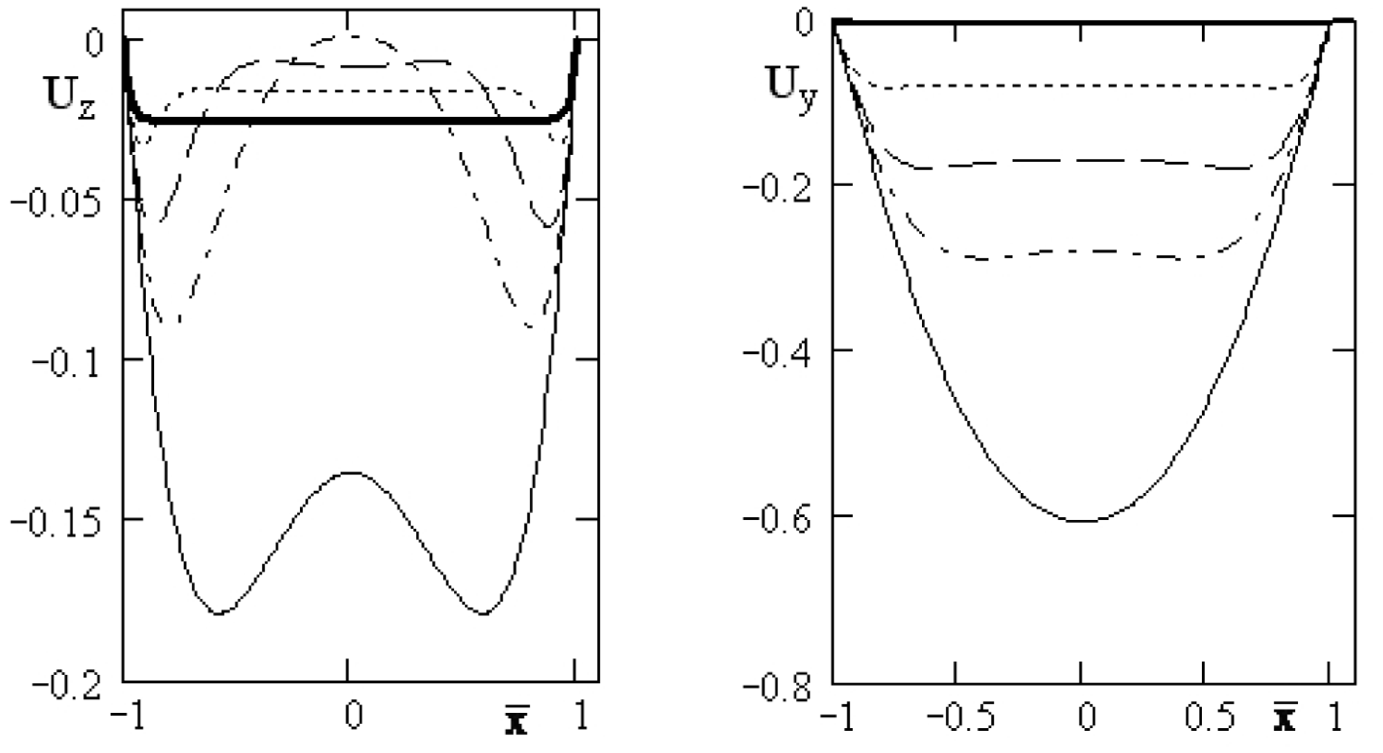
According to the above EMHD theory of plasma in a planar channel, the diagram of the longitudinal velocity $U_{{\it\tau}}=(U_{y},U_{z})$ is a spatial curve and, therefore, it is characterized by two profiles $U_{y}(\bar{x})$ , $U_{z}(\bar{x})$ , $\bar{x}=x/\ell$ , $|\bar{x}|\leqslant 1$ , where $\ell$ is the half-width of the channel. Figure 2 shows the $U_{z}$ and $U_{y}$ diagrams (in the units $\ell ^{2}\partial p_{{\it\Sigma}}/\partial z/{\it\mu}_{{\it\Sigma}}$ ) for the fixed values $\mathit{Ha}=40$ and ${\it\Gamma}=10^{-2},5,20,50,200$ . For ${\it\Gamma}=10^{-2}$ , the $U_{z}$ diagram practically coincides with the Hartmann profile (7.7) for $\mathit{Ha}=40$ , and we have $U_{y}(\bar{x})\cong 0$ (in figure 2, the $U_{y}$ curve for ${\it\Gamma}=10^{-2}$ merges with the axis $\bar{x}$ ), which is consistent with the MHD limit of § 7. As ${\it\Gamma}$ increases, the profile $U_{z}(\bar{x})$ changes significantly: near-wall flows appear ( ${\it\Gamma}=5,20$ ), which, upon further increase of ${\it\Gamma}$ ( ${\it\Gamma}=50$ ), become separated by a ‘dead’ zone $|\bar{x}|\leqslant 1$ with almost no motion of plasma along the axis $z$ , and then ( ${\it\Gamma}=200$ ) these flows merge to form a new flow whose $U_{z}$ curve tends, as ${\it\Gamma}\rightarrow +\infty$ , to the Poiseuille parabola $(\bar{x}^{2}-1)/2$ , $|\bar{x}|\leqslant 1$ , which does not depend on $\mathit{Ha}$ and ${\it\Gamma}$ . If the fixed value of $\mathit{Ha}$ is increased, then for sufficiently large $\mathit{Ha}\geqslant 100$ the plasma in the ‘dead’ zone starts moving in the positive direction along the axis $z$ , which produces counterflows in the channel, while the width of the ‘dead’ zone drastically increases and becomes comparable to the channel half-width, and the near-wall velocity of the plasma increases sharply.

Figure 2.

${\it\Gamma}=10^{-2}$ (——);  ${\it\Gamma}=5$ ( $\cdots \cdots$ );  ${\it\Gamma}=20$ (– – –);  ${\it\Gamma}=50$ (— ⋅ —); ${\it\Gamma}=200$ (——).

The $U_{y}$ diagram in figure 2 exhibits a strong deviation (for suitable $\mathit{Ha}$ , ${\it\Gamma}$ ) of the flow from the direction of the pressure antigradient. For instance, the deflection angle ${\it\alpha}=\arctan (U_{y}/\left|U_{z}\right|)$ in the ‘dead’ zone ( ${\it\Gamma}=50$ ) reaches the value $-{\rm\pi}/2$ , and for large $\mathit{Ha}$ , its absolute value becomes greater than ${\rm\pi}/2$ , if there are counterflows. For small ${\it\Gamma}$ ( ${\it\Gamma}=10^{-2}$ ) and large ${\it\Gamma}\geqslant 200$ , $U_{y}$ is practically equal to zero and there is no hydrodynamic ‘Hall effect’.

It is interesting to note that the deviation of the mean flow velocity $\left\langle U_{{\it\tau}}\right\rangle$ from the pressure antigradient is much smaller than the local deviations. From figure 3, which shows the level lines of the deflection angle ${\it\alpha}=\arctan (U_{y}/\left|U_{z}\right|)$ for isothermal plasma, we see that this angle does not exceed ${\it\alpha}_{\infty }=-0.63$ , in view of (2.3) (see § 8),  which is about half of ${\rm\pi}/2$ in absolute value. At the same time, near the axes $\mathit{Ha}=0$ and ${\it\Gamma}=0$ , the deviation angle is almost equal to zero, and it increases sharply with the distance from these axes, turning smoothly into a large plateau (where ${\it\alpha}\cong {\it\alpha}_{\infty }$ ) formed by values $\mathit{Ha}\gg 1$ , ${\it\Gamma}\gg 1$ .

Figure 3.

Level lines of the deviation angle ${\it\alpha}$ .

Note that the two-frequency nature of the steady flow in a planar channel is not easily perceived, since figure 1 and the asymptotic formulae (7.5) indicate that the profile oscillations are revealed only in distant decimal digits.

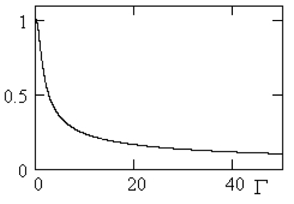
Thus, taking into account the two-fluid plasma structure results in a qualitatively different picture of steady flow in a planar channel for ${\it\Gamma}\gg 1$ . Another important fact is that the MHD theory substantially underestimates the boundary layer thickness. The graph of the ratio ${\rm\Delta}\ell _{MHD}/{\rm\Delta}\ell$ in figure 4 shows that for ${\it\Gamma}\geqslant 2.6$ the MHD boundary layer value is several times smaller that of the EMHD, while for ${\it\Gamma}\geqslant 51.9$ it is tens times smaller, and for large ${\it\Gamma}$ the ratio of the boundary layers is approximately equal to ${\it\Gamma}^{-1/2}{\it\mu}_{{\it\Sigma}}^{1/2}(2{\it\mu}_{+})^{-1/2}\cong (2{\it\Gamma})^{-1/2}$ .

Figure 4.

${\rm\Delta}\ell _{MHD}/{\rm\Delta}\ell$ .

It should be emphasized that the condition ${\it\Gamma}\gg 1$ is usually satisfied for gas plasma, while the opposite condition ${\it\Gamma}\ll 1$ holds for liquid metal plasma. Therefore, in the latter case, the flow in a planar channel is described with great accuracy by the Hartmann solution (7.7), which is unsuitable for gas plasma. Let us give some examples of typical values of ${\it\Gamma}=(H_{0}T_{e}^{3/2}/n_{i})0.632\times 10^{6}$ ( $H_{0}$ in G, $T_{e}$ in $\text{K}$ ) for some types of gas plasma:

1. (i) for the constriction Z-pinch and plasma focus in deuterium with (Imshennik & Bobrova Reference Imshennik and Bobrova1997) ${\it\rho}\sim 10^{-4}~\text{g}~\text{cm}^{-3}$ , $H_{0}\sim 2.8\times 10^{6}~\text{G}$ , $T_{e}\sim 6.5~\text{keV}$ , we have ${\it\Gamma}\sim 3.87\times 10^{4};$

2. (ii) for the stationary plasma thruster (SPT), working on xenon, with (Morozov Reference Morozov2010) $n_{i}\sim 2\times 10^{13}~\text{cm}^{-3}$ , $H_{0}\sim 2\times 10^{2}~\text{G}$ , $T_{e}\sim 20~\text{eV}$ , we have ${\it\Gamma}\sim 1.4\times 10^{3};$

3. (iii) for the solar wind plasma with ${\it\rho}\sim 10^{-23}~\text{g}~\text{cm}^{-3}$ , $H_{0}\sim 10^{-4}~\text{G}$ , $T_{e}\sim 1~\text{eV}$ , we have ${\it\Gamma}\sim 1.32\times 10^{7}.$

The mathematical reason for the significant differences between the EMHD and the MHD theories of plasma in a planar channel is the complex structure of the tensor of ‘Hall terms’ $\unicode[STIX]{x1D652}$ , which in the MHD theory is equal to zero, thereby ensuring the simplicity of the Hartmann flow, whereas in the EMHD theory this tensor essentially differs from zero due to (3.3) and (3.4). Still, the effect of ‘locking’ the plasma flow in the strong magnetic field limit remains: from (6.10), it follows that for ${\it\Gamma}\rightarrow \infty$ , $\mathit{Ha}\rightarrow \infty$ , ${\it\Gamma}/\mathit{Ha}=\text{const.}$ , we have $U_{{\it\tau}}\rightarrow 0$ on $[-\ell ,\ell ]$ .

Finally, we note that for $\mathit{Ha}\ll 1$ the differences between the EMHD and the MHD theories disappear. In this case, the Hartmann solution practically coincides with the Poiseuille parabola, and the same is true for any ${\it\Gamma}>0$ and the EMHD diagrams of  $U_{{\it\tau}}$ .