Sample collection and data acquisition

Hyperspectral image acquisition for spider mite infestation was conducted in the Predatory Mite Research Group of the Institute of Plant Protection, Chinese Academy of Agricultural Sciences, Beijing, China. Two-week-old host bean plants (Phaseolus vulgaris L.) and T. urticae were cultivated and maintained under the conditions of 25 ± 1℃, 70 ± 5% relative humidity and L14:D10 photoperiod. Fifteen host plant seedlings with uniform appearance and growth conditions were selected, among which 10 plants were designated as the treatment group. The exact count of 200 T. urticae was rigorously verified using a stereomicroscope, and they were individually transferred onto the leaves using a fine brush to ensure accurate initial infestation levels, while the remaining five plants served as the healthy control group. For each plant, the first two emerged leaves (the primary leaves) were selected for continuous observation and imaging throughout the study period. These selection criteria ensured that all monitored leaves were at the exact same developmental stage and physiological age, thereby providing a highly uniform background spectral signature. After infestation, all plants were cultivated under same conditions for 7 consecutive days. Hyperspectral data were measured twice a day, at 7:00 AM and 7:00 PM, under consistent measurement environments (i.e. a completely dark room, uniform halogen lighting, and a fixed camera-to-sample distance). Based on infestation days of the pest mite on plants, the treated groups were categorised into three levels of ‘Mild’, ‘Middle’, and ‘Severe’, with further subdivisions as follows: ‘Mild’ into ‘Mild 1’ and ‘Mild 2’; ‘Middle’ into ‘Middle 1’ and ‘Middle 2’; and ‘Severe’ into ‘Severe 1’, ‘Severe 2’, and ‘Severe 3’. The infestation levels were classified by integrating macroscopic visual symptoms, such as leaf colour and contour alterations, with their distinct spectral signatures. These categories were assigned sequence numbers from 1 to 7, with the healthy control group designated as No. 8 for reference.

The optical detection equipment utilised in this study consisted of the portable HSI spectrometer Hc-6010 (custom-developed and manufactured by the Changchun Institute of Optics, Fine Mechanics and Physics, Chinese Academy of Sciences, Changchun, China). The hyperspectral camera was configured to operate in the visible-to-NIR range (400–1,000 nm) captured spectral resolution of 300 bands. Four 50-W halogen lamps (manufactured by OSRAM, Germany) were installed on both sides along the x-axis with four on each side to illuminate the scanning line. The acquired hyperspectral images had a resolution of 480 × 1200 pixels, with each scan measuring three to five leaves. The movable platform set-up was illustrated in fig. 1. The system’s spatial coordinate system is defined by the physical scanning process. The x-axis represents the spatial width covered by the spectrometer’s slit, which remains fixed in its orientation. The y-axis represents the scanning direction (motion axis), where the image length is generated as the camera translates linearly over the samples. A hyperspectral camera was mounted centrally at the top, while a conveyor belt and motor were installed along the x- and y-axes to facilitate camera movement. The y-axis represented the distance between samples, and the lens-to-sample distance was fixed at 300 mm to ensure optimal focus and resolution. The total length of the x-axis was 500 mm, and during the experiments, the camera moved 300 mm at a speed of 150 mm/s to capture line-scan images. For visualisation, composite RGB images were generated by selecting the 120th, 65th, and 45th channels as the R, G, and B channels, respectively. Representative RGB images synthesised from the hyperspectral data are shown in fig. 2. The acquired HSI data were analysed using the spectral library in Python 3.10. Several specialised libraries were employed to facilitate the workflow: Spectral Python was used for hyperspectral image reading and visualisation; NumPy and Pandas were utilised for numerical operations and data structuring; Scikit-learn was applied for data normalisation and classical machine learning tasks; and PyTorch was used for the development and training of the deep learning models.

Figure 1.

The overview of hyperspectral measurement system with camera and plant.

Figure 2.

Time-series pseudo-RGB images (channels 120, 65, 45) of bean leaves under progressive T. urticae infestation, ranging from healthy (left) to severe (right). The white square represents the standard reflectance panel for calibration.

Hyperspectral image data preprocessing

The hyperspectral image data were put through the preprocessing pipeline, as shown in fig. 3. A weighted mean square error (WMSE) algorithm was employed to eliminate outliers in the spectral dimension (Hu et al., Reference Hu, Jin, Wang, Zhang, Kwong and Kuo2017). Since the noise-free hyperspectral image was unknown, the mean square error (MSE) for each spectral band of the original hyperspectral image was considered. A weight w_i was assigned to the MSE of each spectral band. The overall MSE of the entire hyperspectral image can thus be represented as the WMSE, as shown in Equation (1).

(1)\begin{equation}WMSE = \frac{1}{c}\mathop \sum \limits_k^c {\left( {{I^k} - {\bar{I}^k}} \right)^2}{\text{ }},\end{equation}

Figure 3.

Spectral curves illustrating the sequential preprocessing pipeline for a representative sample group. The subplots (from left to right) display the original spectra, outlier rejection based on WMSE, multivariate scatter correction (MSC), Savitzky–Golay filtering, and the final preprocessed mean spectrum with variance bounds (red dashed lines).

In the equation, C represents the number of channels in the hyperspectral image, while ${I^k}$ and ${\bar I^k}$ denote the greyscale value of the kth spectral band of the hyperspectral image and the mean greyscale value of that band, respectively. Subsequently, for each pixel’s spectral data, a query is performed: if the pixel value falls within the range of ${I^k}$ ± WMSE.

By placing the calibrated standard reflectance panel around the target, both the target’s hyperspectral image and the hyperspectral image of the standard reflectance panel can be collected (Rabatel et al., Reference Rabatel, Al Makdessi, Ecarnot and Roumet2017). Utilising Equation (2) in conjunction with the known calibrated spectra allowed for the normalisation of the hyperspectral image, which can partially correct for radiometric errors and transform the image greyscale values between 0 and 1.

(2)\begin{equation}R = \frac{{({I_o} - {I_b})}}{{{I_w} - {I_b}}},\end{equation}

In this context, ${I_{\text{O}}}$ represents the unprocessed hyperspectral image data, ${I_b}$ denotes the dark noise from the imaging chip of the spectrometer, which is typically collected by covering the lens, and ${I_w}$ refers to the hyperspectral image data of the area where the standard reflectance panel is located.

Multivariate scatter correction (MSC) operates based on a spectral matrix from a set of samples. As a scatter correction technique, MSC was applied to minimise the influence of light scattering caused by leaf surface irregularities and light path variations, thereby enhancing the spectral features related to the physiological state of the plants. The specific algorithmic process for calculation is as follows Equation (3) (Roessner et al., Reference Roessner, Segl, Heiden and Kaufmann2001). The average of all spectral data was obtained and referred to as the ideal spectrum.

(3)\begin{equation}{\bar I^k} = \frac{1}{c}\mathop \sum \limits_{i = 1}^m \mathop \sum \limits_{j = 1}^n {I_{ij}}\end{equation}

We performed a univariate linear regression of each sample’s spectrum against the average spectrum to solve the least squares problem, obtaining the baseline shift and offset for each sample, as shown in Equation (4).

(4)\begin{equation}{I^k} = {A_k}{\bar I^k} + {B_k}\end{equation}

Subsequently, the spectrum of each sample was corrected by subtracting the obtained baseline offset and dividing by the intercept, as shown in Equation (5).

(5)\begin{equation}{\hat I^k} = \frac{{{I^k} - {B_k}}}{{{A_k}}}\end{equation}

After correcting the edge bands of the hyperspectral image, significant noise was present due to the low signal-to-noise ratio of the sensor. The original 300 spectral channels were trimmed by 25 channels from both the start and end of the spectrum, leaving 250 channels for analysis. Savitzky–Golay filtering was then used for denoising data (Ruffin et al., Reference Ruffin, King and Younan2008; Ning et al., Reference Ning, Tan, Li, Jiao and Wen-Hao2020).

Hyperspectral image data dimensionality reduction

The processing of hyperspectral image data was challenged by the large volume of data storage and the increased computational complexity. By focusing on small samples, we considered dimensionality reduction for hyperspectral images in small sample scenarios, which can effectively improve the classification accuracy of hyperspectral images. According to electromagnetic wave theory, the absorption features indicated physical things, such as for water, chlorophyll, certain gases, and minerals (Mahlein et al., Reference Mahlein, Kuska, Behmann, Polder and Walter2018). To highlight certain features of the spectral band calculations, the plant indices are listed in table 1.

Table 1.

The formulae and calculation details of vegetation indices used for plant analysis

Traditional indices use only 3–10 specific spectral bands (wavelengths), wasting the rest and yielding illumination-sensitive, unquantified proxies that may blur useful gradients (Shirzadifar et al., Reference Shirzadifar, Bajwa, Nowatzki and Shojaeiarani2020). To address these limitations and learn the intrinsic low-dimensional features from the full hyperspectral data, we therefore chose super-pixel PCA method (SPCA; fig. 4). Unlike traditional empirical methods that rely on selecting specific discrete wavelengths, SPCA transforms the highly correlated high-dimensional spectral data (400–1,000 nm) into a reduced set of orthogonal principal components. This transformation effectively fuses and retains the most informative variance across the entire spectrum. Consequently, it inherently captures critical physiological changes, such as chlorophyll degradation in the red-edge (680–760 nm) and cellular damage in the NIR (700–1000 nm) regions, without losing hidden features to manual band selection. Furthermore, since SPCA relies on spatial segmentation, we compared the performance of different super-pixel algorithms, including Felzenszwalb, SLIC, Quickshift and Compact Watershed (fig. 5). Considering the overall performance, SLIC was selected as the optimal algorithm for this study. The specific implementation details of the SLIC-based spatial partitioning are provided in table 2.

Figure 4.

Schematic of super PCA-based dimensionality reduction for hyperspectral images (HSIs).

Figure 5.

Felzenszwalb’s method, SLIC, Quickshift, Compact Watershed super-pixel segmentation spatial dimension results.

Table 2.

SLIC-based super-pixel Segmentation for hyperspectral data

Deep neural network for early detection of T. urticae on the leaf

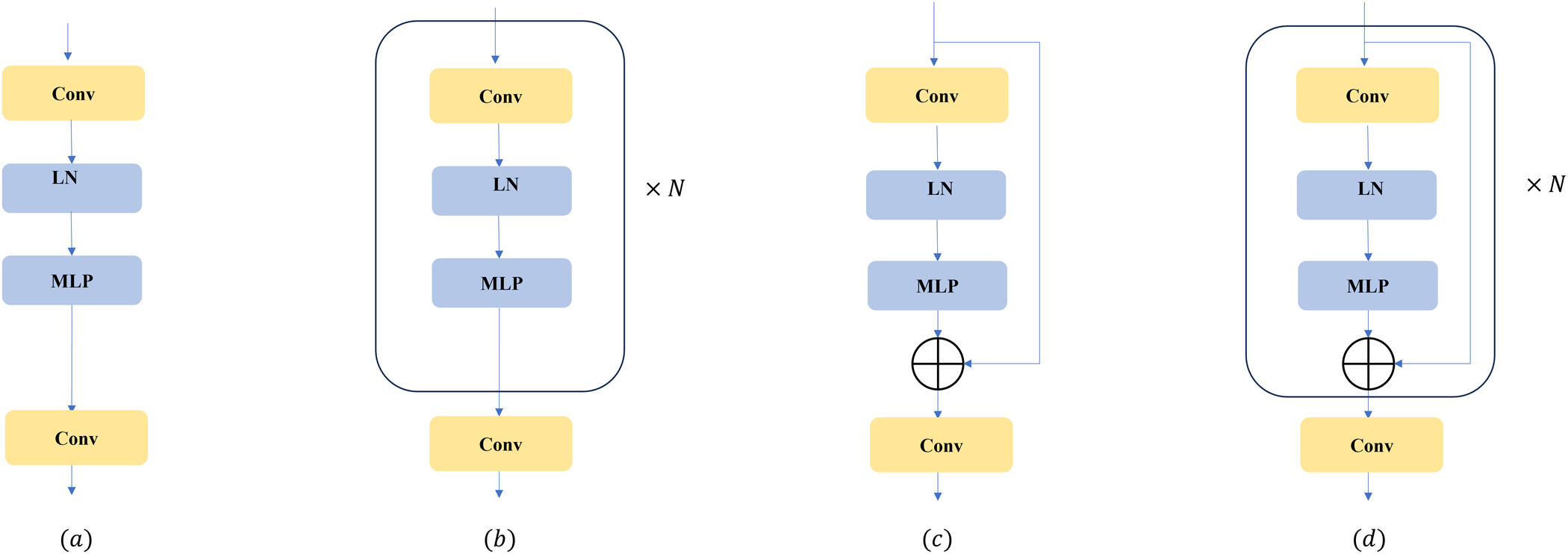
The CNN model and residual neural network were used in data classification tasks. When directly applying the network to small-sample hyperspectral image classification, the network may fail to converge due to the vanishing gradient caused by the deepening of the network.

In this study, the spatial dimension of hyperspectral images cannot be overlooked. The pest detection model took image patches as input and generates predicted labels for these patches. Given the ith pixel to be classified, its neighbouring pixels may differ in terms of illumination, viewpoint, and category. Considering such spatial variations, a spectral-spatial attention mechanism in a DCNN (DCNN + SSA) was designed. The overall framework of the proposed DCNN + SSA classification method was illustrated in fig. 6. This model has two key features, including the improvement of the discriminative power of the learned features and the integration of attention modules in both spatial and spectral dimensions (Mahlein et al., Reference Mahlein, Steiner, Hillnhütter, Dehne and Oerke2012; Pandey et al., Reference Pandey, Singh, Khan and Semwal2022; Bao et al., Reference Bao, Zhou, Bhuiyan, Adhikari, Tuxworth, Ford and Gao2024). The detailed architecture of the network, specifically highlighting the SSA modules, is presented in fig. 7. During the pest detecting process, infested areas typically exhibited distinct texture and colour characteristics, so the spatial attention aided the model in identifying and differentiating pest-affected regions from healthy leaves. The specific structure of the DCNN + SSA network can be expressed mathematically through the following functional computation:

(6)\begin{equation}{C^i} = f\left( {\sum\nolimits_j {\left( {{W^{i*}}} \right) + {b^i}} } \right),\end{equation}

Figure 6.

Outline of the proposed spatial-spectral attention super PCA-based HSI classification framework.

Figure 7.

Outline of the proposed spatial-spectral attention super PCA-based HSI classification.

In this context, ${C^i}$ represents the ith channel of the convolutional feature map, ${W^i}$ denotes the ith convolutional kernel, ${b^i}$ is the bias term for the ith feature map, and ${X^j}$ refers to the jth input feature.

Loss function can be expressed as following:

(7)\begin{align} {\text{L = }}& {\mathcal{L}^{{\text{spectral}}}} + {\mathcal{L}^{{\text{spatial}}}} \nonumber \\ &{\text{ = }} - \frac{1}{m}\sum\nolimits_{i = 1}^m {[{y_i}log(\hat y_i^{{\text{spectral}}}) + (1 - {y_i})\log (1 - \hat y_i^{{\text{spectral}}})]}, \nonumber \\ & \quad - \frac{1}{m}\sum\nolimits_{i = 1}^m {[{y_i}log(\hat y_i^{{\text{spatial}}}) + (1 - {y_i})\log (1 - \hat y_i^{{\text{spatial}}})]} \end{align}

Model deployment and training

Due to PyTorch’s dynamic debugging, visualisation capabilities, and efficient GPU acceleration, all neural network models in this study were developed based on this Python open-source machine learning framework. The hyperspectral data from groups 1 to 8 were preprocessed, and after applying PCA and SPCA, they were labelled to train the DCNN and DCNN + SSA models, with the number of epochs set to 100. To enhance the model’s generalisation ability, the data were divided into several patches, each with a size of 100 × 100 × 30 for the hyperspectral images.

K-fold cross-validation was used as a commonly adopted evaluation strategy to test the model’s robustness and generalisation ability. When applying K-fold cross-validation, evaluation results were obtained from different subsets of the dataset, and reported by averaging all evaluation outcomes. Monte Carlo sampling was used to sample from patches, with a total dataset size of 1000 image patches. Among these, 800 patches were allocated to the training set, 100 patches to the validation set, and 100 patches to the test set. The hardware platform for model training was as follows: CPU: Intel i7-14700KF, GPU: NVIDIA RTX-4090 24GB, with 48GB system memory.

Evaluate method

Overall accuracy (OA) and Kappa coefficient were commonly used metrics to evaluate the performance of classification models, when Kappa coefficient provided a more reliable evaluation than simple OA in such cases (Li et al., Reference Li, Hong, Ni, Li, Wang, Zheng and Lin2014; Wang et al., Reference Wang, Das, Pang and Liang2021). In this study, class imbalance existed, as healthy pixels significantly exceeded the pest-infected pixels in the hyperspectral images of early-infected leaves. As a result, OA may give inflated results, and the classifier may still achieve a high OA even if it did not effectively recognise the rare class. The formula was as follows:

(8)\begin{equation}\mathrm{OA} = \frac{\text{pixels classified correctly}}{\text{total pixels}} = \frac{\sum_{i=1}^{C} {\text{TP}}_i}{\sum_{i=1}^{C} {\text{Total}}_i}\end{equation}

The Kappa coefficient was used to measure the agreement between classification results and random classification results. The formula is as follows:.

(9)\begin{equation}{{\kappa }} = \frac{{{P_o} - {P_e}}}{{1 - {P_e}}}\end{equation}

${P_{o}}$ is the observed agreement (the proportion of actual classifications that match the predicted classifications), which is the same as the OA. ${P_e}$ is the expected agreement, which represents the probability of random agreement between categories under the assumption of completely random classification. Kappa coefficient takes into account the effect of random agreement, providing a more accurate assessment of the classifier’s performance, particularly in cases of class imbalance, where it reduces the overestimation produced by OA.