1. Introduction
Flow control is a rapidly evolving interdisciplinary field comprising many disciplines, such as fluid mechanics, technological innovations for sensors and actuators, control theory, optimization and machine learning. It has potential for use in a vast range of engineering applications, including aerodynamic of cars, trucks, trains, wind turbines and gas turbines, as well as medical equipments and chemical plants. Flow control is employed to reduce aerodynamic drag for cars (Beaudoin & Aider Reference Beaudoin and Aider2008; Gillieron & Kourta Reference Gillieron and Kourta2010; Joseph et al. Reference Joseph, Amandolese, Edouard and Aider2013), to find alternative lift-off and take-off configurations for aircraft and to improve mixing efficiency (M’Closkey et al. Reference M’Closkey, King, Cortelezzi and Karagozian2002).
There have been many successful implementations of passive and active open-loop flow control (Fourrié et al. Reference Fourrié, Keirsulck, Labraga and Gillieron2010; Joseph, Amandolese & Aider Reference Joseph, Amandolese and Aider2012; Gautier & Aider Reference Gautier and Aider2013b ). Closed-loop control offers great potential for increased robustness and efficiency and is currently the subject of increasing ongoing research efforts (Beaudoin et al. Reference Beaudoin, Cadot, Aider and Wesfreid2006; Henning & King Reference Henning and King2007; Pastoor et al. Reference Pastoor, Henning, Noack, King and Tadmor2008; Tadmor et al. Reference Tadmor, Lehmann, Noack, Cordier, Delville, Bonnet and Morzyński2010; Brandt et al. Reference Brandt, Sipp, Pralits and Marquet2011; Semeraro et al. Reference Semeraro, Bagheri, Brandt and Henningson2011; Gautier & Aider Reference Gautier and Aider2013a ). In experiments, most closed-loop controls are adaptive (Beaudoin et al. Reference Beaudoin, Cadot, Aider and Wesfreid2006; Henning & King Reference Henning and King2007; Gautier & Aider Reference Gautier and Aider2013a ) and based on slowly varying periodic forcing. In-time control remains very challenging because of the nonlinear nature of fluid phenomena. Most model-based control designs are based on a (locally) linear reduced-order model and ignore frequency cross-talk. The low-dimensionality of the model is key for robustness and online capability in experiments (Bergmann & Cordier Reference Bergmann and Cordier2008; Noack, Morzyński & Tadmor Reference Noack, Morzyński and Tadmor2011; Hervé et al. Reference Hervé, Sipp, Schmid and Samuelides2012). Only a few control-oriented reduced-order models address frequency cross-talk (Luchtenburg et al. Reference Luchtenburg, Dirk, Gunther, Noack, Rudibert and Gilead2009; Luchtenburg Reference Luchtenburg2010).
The challenges of model-based control design have led us to search for model-free control laws using machine learning methods such as evolutionary algorithms (Wahde Reference Wahde2008) or artificial neural networks (Lee et al. Reference Lee, Kim, Babcock and Goodman1997). These have been successfully used in many disciplines such as bio-informatics, medicine and computer science (Harik Reference Harik1997; Ferreira Reference Ferreira2001; Shah-Hosseini Reference Shah-Hosseini2009).
This study builds on and extends pioneering work on machine learning based control by Rechenberg (Reference Rechenberg1994), Lee et al. (Reference Lee, Kim, Babcock and Goodman1997) and Milano & Koumoutsakos (Reference Milano and Koumoutsakos2002) to name a few. The relevant techniques to achieve such a goal are genetic algorithms (GA), artificial neural networks (ANN) and genetic programming (GP). GAs were first suggested for flow control by Rechenberg (Reference Rechenberg1994). They have been used in fluid mechanics for shape optimization (Toivanen et al. Reference Toivanen, Makinen, Periaux and Cloud Cedex1999; Gardner & Selig Reference Gardner and Selig2003), to optimize feedback control schemes for wall turbulence (Morimoto et al. Reference Morimoto, Iwamoto, Suzuki and Kasagi2002), to find optimal wing configurations in insect flight (Berman & Wang Reference Berman and Wang2007), to minimize drag on a cylinder in numerical simulations and to fine tune a control law to minimize drag in an experimental turbulent channel flow (Milano & Koumoutsakos Reference Milano and Koumoutsakos2002). It should be noted that in these examples featuring GA the goal is optimizing tuning parameters. The algorithm is used to search for the best parameters of a given, set control law. As GA can tunes parameters, it can only be employed to optimize given designs of control laws. Model-free control using machine learning methods has been pioneered by Lee et al. (Reference Lee, Kim, Babcock and Goodman1997) using ANN (Kim Reference Kim2003). While ANN can approach solutions by a complex combination (described by the network structure) of sigmoids functions, the performance of such an algorithm depends on the learning scheme implemented. If the classical errors back-propagation learning scheme is implemented, then the search algorithm is gradient based and thus sensitive to local minima. Genetic algorithms can be used to avoid this problem.
The third technique (GP) is used to find a control law optimizing a cost function. As with GA, an exploration of the search space is achieved alongside cost functional minimization. The main difference and advantage compared to GA is that GP is optimizing arbitrary functions, allowing its use in a model-free manner and thus exploring a larger search space. When comparing GP to ANN the advantage lies in the output of the GP, which is the expression of the function. This allows the study of the control law and gaining knowledge of the flow physics.
These algorithms are commonly used in many logistic and pattern recognition tasks. However, GP-based control laws are rare in experimental closed-loop flow control. One of the obstacles to application of GP to experimental flow control is that a large number of experiments is required to fulfil the criterion for statistical convergence. Recently, Duriez et al. (Reference Duriez, Parezanovic, Laurentie, Fourment, Delville, Bonnet, Cordier, Noack, Segond, Abel, Gautier, Aider, Raibaudo, Cuvier, Stanislas and Brunton2014) used GP to find closed-loop control laws in flow control problems. This approach proved surprisingly effective when applied to complex dynamical systems for closed-loop turbulence control in an experiment (Parezanovic et al. Reference Parezanovic, Laurentie, Duriez, Fourment, Delville, Bonnet, Cordier, Noack, Segond, Abel, Shaqarin and Brunton2014).
The objective of the present study is to use GP to control a separated flow for the first time. The control objective is chosen to be the reduction of recirculation bubble area downstream a backward-facing step (BFS). In § 2, the experiment is described. The genetic programming control is presented in § 3. The closed-loop control results are discussed and benchmarked against periodic forcing in § 4. Section 5 summarizes the main finding and provides future research directions.
2. Experimental set-up
2.1. Water tunnel
Experiments were carried out in a hydrodynamic channel in which the flow is driven by gravity. The flow is stabilized by divergent and convergent sections separated by honeycombs. The quality of the main stream can be quantified in terms of flow uniformity and turbulence intensity. The standard deviation
 ${\it\sigma}$
is computed for the highest free-stream velocity featured in our experimental set-up. We obtain
 ${\it\sigma}=5.9\times 10^{-4}~\text{m}~\text{s}^{-1}$
which corresponds to turbulence levels of
 ${\it\sigma}/U_{\infty }=2.3\times 10^{-3}$
. For the present experiment the flow velocity is
 $U_{\infty }=7.3\times 10^{-2}~\text{m}~\text{s}^{-1}$
giving a Reynolds number based on step height and kinematic viscosity of
 $\mathit{Re}_{h}=U_{\infty }h/{\it\nu}=1350$
. This Reynolds number was chosen because of the limitations of the injection system.
2.2. Backward-facing step geometry
The BFS is considered a benchmark geometry for the study of separated flows: separation is imposed by a sharp edge creating a strong shear layer susceptible to Kelvin–Helmholtz instability. Upstream perturbations are amplified in the shear layer leading to significant downstream disturbances. This flow has been extensively studied both numerically and experimentally (Armaly et al.
Reference Armaly, Durst, Pereira and Schonung1983; Hung, Parviz & John Reference Hung, Parviz and John1997; Beaudoin et al.
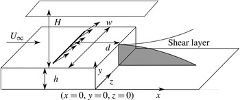
Reference Beaudoin, Cadot, Aider and Wesfreid2004). The BFS geometry and the main geometric parameters are shown in figure 1. BFS height is
 $h=1.5\times 10^{-2}~\text{m}$
. Channel height is
 $H=7\times 10^{-2}~\text{m}$
for a channel width
 $w=15\times 10^{-2}~\text{m}$
. The vertical expansion ratio is
 $A_{y}=H/(h+H)=0.82$
and the spanwise aspect ratio is
 $A_{z}=w/(h+H)=1.76$
. The injection slot is located
 $d/h=2$
upstream of the step edge. The boundary layer thickness at the step edge is
 ${\it\delta}=1.3h$
.
Sketch of the BFS geometry, position of the slotted jet and definition of the main parameters.

2.3. Sensor: two-dimensional real-time velocity fields computations
The sensor is built on a real-time computation of the vector fields. The velocity fields are computed based on snapshots from the seeded flow. The seeding particles are
 $20~{\rm\mu}\text{m}$
neutrally buoyant polyamid particles. They are illuminated by a laser sheet created by a 2 W continuous laser beam operating at
 ${\it\lambda}=532~\text{nm}$
. Images of the vertical symmetry plane are recorded using a Basler acA 2000–340 km 8 bit CMOS camera. Velocity fields are computed in real-time on a Gforce GTX 580 graphics card. The algorithm used to compute the velocity fields is based on a Lukas–Kanade optical flow algorithm called FOLKI developed by Le Besnerais & Champagnat (Reference Le Besnerais and Champagnat2005). Its offline and online accuracy has been demonstrated and detailed by Champagnat et al. (Reference Champagnat, Plyer, Le Besnerais, Leclaire, Davoust and Le Sant2011) and Gautier & Aider (Reference Gautier and Aider2014b
). Furthermore this acquisition method was successfully used in Davoust, Jacquin & Leclaire (Reference Davoust, Jacquin and Leclaire2012), Gautier & Aider (Reference Gautier and Aider2013a
) and Gautier & Aider (Reference Gautier and Aider2014a
). Velocity fields are computed over an area of
 $(17.2\times 4.6)\times 10^{-4}~\text{m}^{2}$
which translates into a
 $(9\times 3)h^{2}$
area. The time between two snapshots yielding one velocity field is
 ${\it\delta}t=10\times 10^{-3}~\text{s}$
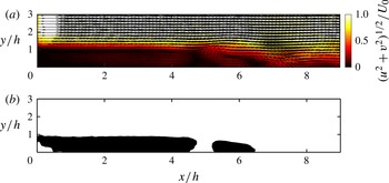
. Forty-two image pairs are processed per second. Figure 2(a) shows a typical example of the instantaneous velocity magnitude field downstream of the step for the uncontrolled flow.
(a) Instantaneous velocity snapshot. Arrows show the instantaneous velocity field while the background colour indicates the magnitude of the instantaneous velocity. The edge of the backward-facing step is at
 $x=0$
and
 $y=1$
. (b) Corresponding instantaneous mapping of the recirculation area. A black dot indicates a velocity vector with negative streamwise velocity.

Recirculation plays a major role in the BFS flow and is overwhelmingly used for flow assessment as well as an objective for the control of flow separation (Chun & Sung Reference Chun and Sung1996; Henning & King Reference Henning and King2007). It has also been shown that the recirculation bubble can be linked to drag (although the relationship is far from trivial) (Dahan, Morgans & Lardeau Reference Dahan, Morgans and Lardeau2012). We choose to evaluate the state of the flow through the instantaneous recirculation area, computed from instantaneous velocity fields, as our input. It is a two-dimensional extension of the more common recirculation length evaluated using wall measurements. The recirculation area and recirculation length have been shown to behave the same way by Gautier & Aider (Reference Gautier and Aider2013a
). The normalized instantaneous recirculation area
 $s(t)$
is computed using
 $$\begin{eqnarray}\displaystyle \left.\begin{array}{@{}c@{}}s(t)=\displaystyle \frac{\displaystyle \int H(-u(x,y,t))\text{d}x\text{d}y}{A_{0}},\\ A_{0}=\displaystyle \frac{1}{T}\displaystyle \int _{0}^{T}A_{uncont}(t)\text{d}t,\end{array}\right\} & & \displaystyle\end{eqnarray}$$
where
 $H$
is the Heaviside function,
 $u(x,y,t)$
is streamwise velocity,
 $A_{0}$
is the time-averaged recirculation area for the uncontrolled flow and
 $A_{uncont}$
is the instantaneous recirculation area for the uncontrolled flow. See figure 1 for
 $x,y,z$
directions. Figure 2(b) shows the instantaneous recirculation area corresponding to the instantaneous velocity field shown on figure 2(b) and computed using (2.1).
2.4. Actuator
Actuation is provided using upstream injection through a spanwise slotted jet as shown in figure 1. The angle between the jet axis and the wall is
 $45^{\circ }$
. The jet flow is induced using a pressurized water tank. It enters a plenum and goes through a volume of glass beads designed to homogenize the incoming flow. The jet amplitude
 $U_{j}$
is controlled by changing tank pressure. Because channel pressure is higher than atmospheric pressure this allows us to provide both blowing and suction. Maximum actuation frequency
 $f_{a}$
is about 2 Hz. To achieve closed-loop control, the control value
 $b=U_{j}/U_{max}$
(
 $U_{max}$
being the maximum jet velocity) is computed as a function of the sensor value
 $s$
inside a Labview project. The specific control laws are derived through genetic programming.
3. Genetic programming control
We propose a generic, model-free, approach to closed-loop control of nonlinear systems. Following Duriez et al. (Reference Duriez, Parezanovic, Laurentie, Fourment, Delville, Bonnet, Cordier, Noack, Segond, Abel, Gautier, Aider, Raibaudo, Cuvier, Stanislas and Brunton2014) we refer to this approach as machine learning control (MLC). Control laws are optimized with regard to a problem-specific objective function using genetic programming (Koza et al.
Reference Koza, Bennett and Stiffelman1999). A first generation of control law candidates
 $b_{i}^{1}(s)$
, called individuals (
 $b_{i}^{1}(s)$
is the
 $i$
th individual of the first generation), is randomly generated by combining user-defined functions, constants and the sensor value
 $s$
(see appendix A). Each individual is evaluated yielding a value for the cost function
 $J$
. A new population
 $b_{i}^{2}$
is then generated by evolving the first generation. The procedure is iterated until either a known global minimum of
 $J$
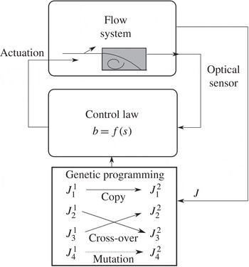
is reached or the evolution is stalled. This process is summarized in figure 3.
Control loop featuring genetic programming. Control laws
 $b(s)$
are evaluated by the flow system. This is done over several generations of individuals. New generations are generated by replication, crossover and mutation.
 $J_{i}^{n}$
refers to the
 $i$
th individual of generation
 $n$
.

3.1. Population generation
The number of individuals inside a generation has a strong influence on the process. While a large number of individuals will certainly lengthen the total time of the experiment, it will also ensure a higher diversity which is known to be a key parameter of all evolving algorithms. In the present study, each generation is made of 500 individuals. This number of individuals is a good compromise between performance and testing time. It has proven to be enough to converge on most single input/single output problems, and is still manageable in terms of total experimental time.
The first individuals
 $b_{i}^{1},1\leqslant i\leqslant 500$
, are generated as expression trees made of user-defined nodes (see appendix A). These nodes are functions (
 $\sin$
,
 $\cos$
,
 $\exp$
,
 $\log$
,
 $\tanh$
), basic operations (
 $+,-,\times ,/$
), constants and the sensor input
 $s(t)$
. The root of the expression tree, i.e. the value returned by the function it defines, is the control value. To build the expression tree, a recursive algorithm is used: a first node is chosen, then for each argument this node can accept, new nodes are added randomly until all terminal nodes do not accept any arguments (constants or sensor). The algorithm is made so that the first generation contains expression trees of different depth and density to ensure diversity in the population. Furthermore all individuals are different.
3.2. Evaluation
Expression trees can be easily written as locator/identifier separation protocol (LISP) expressions. The evaluation is done by translating the LISP expression, for example
 $(+(\sin s)(/\,2.343s))$
, into a control law inside the software responsible for the real-time closed-loop control (
 $b=\sin (s)+(2.343/s)$
). The numerical value used to grade each individual is the cost function
 $J$
linked to the control problem. In our case the goal is to reduce the recirculation area over the evaluation time with a penalization by the energy used for the actuation:
 $$\begin{eqnarray}J=\langle s\rangle _{T}+w\langle |b|\rangle _{T}^{2}>0,\end{eqnarray}$$
where
 $T$
is the evaluation time (
 $T=60~\text{s}$
). The first component quantifies the state of the flow and averages the sensor
 $s(t)$
during the evaluation time. Here
 $s(t)$
is normalized by the time-averaged uncontrolled recirculation area
 $A_{0}=\langle s\rangle _{T}$
. Normalization is important as it allows corrections taking into account variations in the flow conditions (i.e. temperature variations, flow rate drifts).
 $A_{0}$
is recomputed every 250 individuals to compensate for any drifts. The second component, weighted by
 $w$
, is tied to actuation energy and is normalized by the maximum jet velocity
 $U_{max}$
. In the following, we choose
 $w=3/2$
, to strongly penalize high actuation costs. Although the choice of
 $w$
is arbitrary, the value represents a trade-off between the gain on area reduction and actuation cost. Setting a low (respectively high) value of
 $w$
means that the performance of the system is much more (respectively less) important than the cost of the control. A balanced value can be derived by evaluating how much one is ready to spend in energy to achieve a given performance. The ratio between performance gain and actuation cost of the most effective open-loop control (see § 4.3) suggests a value close to
 $w=3/2$
. This value was found to strike a good balance between recirculation reduction and actuation cost. It should be noted that
 $J$
could be amended to further constrain the control laws, for example it could be modified to penalize non-zero net mass flux actuation (by penalizing the difference between blowing and suction fluxes) or strong variations in actuation intensity (by penalizing the derivative of the control signal).
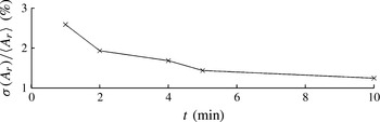
The evaluation time is also a key parameter as it will determine how long the whole experiment will last. Figure 4 shows that a one minute evaluation is enough to get significant statistics for an evaluation of
 $J$
good enough to discriminate between individuals by performance. As time is spent refilling the jet supply tank, the time between two evaluations varies and can reach two minutes. Approximately 1000 individuals, i.e. two generations, are evaluated over 24 h.
Standard deviation of mean recirculation area in percent over ten evaluations for different evaluation periods.

Because control laws can be constants (e.g.
 $b=0.2+0.17$
) or be outside the actuator’s operating range (e.g.
 $b=\exp (9.87)+(s\times s)$
), each control law is pre-evaluated before it is applied to the flow. If it is found to saturate the actuator, it is assigned a very high cost. This step takes a few milliseconds and is done to ensure faster convergence by discarding uninteresting functions. Because of the random nature of the first generation most individuals saturate the actuator.
3.3. Breeding of subsequent generations and stop criteria
Once every individual of the current generation has been evaluated, they are sorted by their cost function value
 $J$
. The five best individuals are evaluated again, the cost values are averaged and the population is sorted again. This re-evaluation procedure is repeated five times to ensure that the value of the best individuals is reliable. The individuals of the next generation are then produced through three different processes. Mechanisms are based on a tournament process: seven individuals are randomly chosen, the individual elected to enter a breeding process is the one with the lowest cost function value. This ensures that the best individuals inside a generation will be used a lot, while less well-performing individuals still have a chance to be part of the next generation. Individuals selected this way will then be either replicated, mutated or crossed to generate the individuals of the next generation. The probabilities of replication, mutation and crossover are respectively 10 %, 20 % and 70 %. This new generation is then evaluated and the whole process is iterated. The process can stop for two reasons. The first one is when
 $J$
reaches 0, which in general does not occur. Most of the time, the process is stopped when the best values of
 $J$
over the population stop improving over several generations.
4. Results
The approach described in § 3 has been applied to the backward-facing step set-up presented in § 2. Generation convergence is analysed in § 4.1. The best control law of the final generation is presented in § 4.2. This control law is compared with open-loop forcing (§ 4.3) and tested for robustness with respect to the Reynolds number in § 4.4.
4.1. Convergence of machine learning control
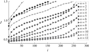
The evolution of the cost function with increasing number of individuals is shown in figure 5 for all twelve generations. All random control laws of the first generation are seen to be ineffective, i.e. produce only cost functions which are worse than the uncontrolled flow (
 $J_{i}^{1}>1$
for all
 $i$
). Considering the large search space created by the many ways one can arrange the node functions, sensor and constants, it is not surprising that a Monte-Carlo process with 500 individuals is ineffective. A few effective control laws can be seen as soon as the second generation. The slope of the cost function
 $J_{i}$
as a function of the index
 $i$
is improved. This clearly shows that the search algorithm is effective in exploring and exploiting the search space defined by the cost function. All subsequent generations perform better than the previous one, i.e.
 $J_{i}^{n+1}<J_{i}^{n}$
. After the 9th generation, the performance of the best individuals appears to converge.
Cost functions of the first 300 individuals in all twelve generations.

The average of the best five control laws
 $J_{[1..5]}^{n}:=(J_{1}^{n}+J_{2}^{n}+J_{3}^{n}+J_{4}^{n}+J_{5}^{n})/5$
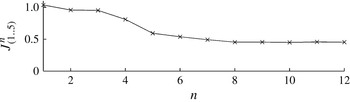
is shown in figure 6 for each generation. Convergence is reached after the 8th generation. A good termination criterion appears to be to stop the iteration once the average of the cost function for the first five individuals no longer improves. In our case the experiment was stopped after no substantial enhancement was obtained in five generations from the eighth to 12th generation. As the number of generations increases the first five control laws become very similar and averaging over them is a more robust measure than taking just the best one.
Cost functions averaged over the five best individuals for each generation.

The evaluation of the 12 generations translates into a week of continuous automatized experiments. At the end of the week, the training phase is finished and an effective, closed-loop control law has been obtained. While a week of experiment is an investment, it has to be compared with the time needed by other methods to obtain a viable real-time closed-loop control, which usually is counted in months. This places this approach in the category of a control algorithm that can be used to obtain a controller in a comparatively small amount of time.
4.2. Analysis of the best control law obtained through genetic programming
The control law
 $b=K(s)$
has a complex mathematical expression:
 $$\begin{eqnarray}b=\exp -0.1138\times \log (\cos (\log (s))-\sin (\cos (\tanh (\sin (s))))).\end{eqnarray}$$
Yet, the graph of the best control law for the final generation has a simple structure as shown on figure 7 for
 $0\leqslant s\leqslant 1$
. The controlled normalized recirculation area is by definition positive,
 $s\geqslant 0$
. Experimentally, the instantaneous recirculation area associated with the best law is found to be always smaller than the averaged uncontrolled region resulting in
 $s\leqslant 1$
. Note that the control law leads to a combination of blowing and suction as a function of
 $s$
.
Graph of the best control law
 $b=K(s)$
(4.1) obtained after 12 generations.

The actuation command
 $b$
has an interesting non-proportional and non-monotonic dependence on
 $s$
with two similar maxima
 $b\approx 0.6$
(injection) and two similar minima
 $b\approx 0.3$
(suction) which shows that it could not be obtained through a linear process. Near uncontrolled values for the recirculation zone (
 $s\sim 1$
), large jet injection reduces the area. This injection decreases with
 $s$
until suction sets in at intermediate values (
 $s\sim 0.73$
). In the post-transient regime (
 $0.12<s<0.32$
), injection increases with recirculation area. For
 $s<0.12$
, suction sets in. Most of the time, injection
 $b\approx 0.5$
occurs. During short periods with low recirculation zones, suction sets in or, at minimum, injection is significantly reduced.
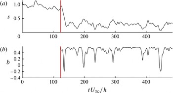
It is interesting to look at the time-series of
 $s(t)$
(figure 8
a) and the corresponding actuation amplitude
 $b(t)$
(figure 8
b) for the best closed-loop control law. Once the control starts at time
 $t=25~\text{s}$
(vertical line) the recirculation area is quickly and strongly decreased down to 20 %, corresponding to a 80 % reduction on average. For
 $0<s<0.3$
, actuation
 $b$
is roughly an affine function of
 $s$
(see figure 7). Figure 8(b) shows that the actuation is indeed a succession of a short period of suction followed by a longer period of blowing (
 $b\approx 0.45$
).
(a) System response
 $s$
to the control law; the vertical line shows when control starts at
 $t=120~\text{s}$
. (b) Corresponding actuation
 $b$
.

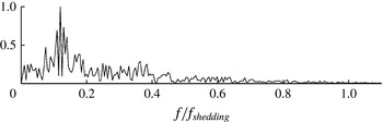
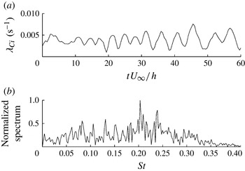
This feedback loop creates oscillations at 0.1 Hz, as observed in figure 8(a,b) and confirmed by the frequency analysis for the actuation signal shown in figure 9. We conjecture that this frequency is the flapping frequency of the recirculation bubble, which is typically an order of magnitude lower than the shear layer shedding frequency (Spazzini et al. Reference Spazzini, Luso, Onorato, Zurlo and Di Cicca2001) (shown in figure 10 b below), as illustrated by figure 9.
Normalized frequency spectrum obtained by Fourier transform of the actuation signal, frequency is normalized by vortex shedding frequency.

 ${\it\lambda}_{Ci}(t)$
signal over 60 non-dimensionalized time units, uncontrolled flow. (b) Normalized frequency spectrum showing a peak at
 $St=0.2$
corresponding to 0.97 Hz.

The 0.1 Hz feedback dynamics is probably triggered by the choice of our input, the instantaneous recirculation area, and the natural flapping frequency. The periodic events of reduced injection or low suction are awarded by the cost function which penalizes the actuation.
It is important to notice that the low-frequency nature of this actuation enables ‘slow’ actuators to positively affect high-Reynolds-number flows. It may remove strong constraints on the actuator in industrial settings which usually deal with high-frequency vortex shedding (typically a few hundred Hz for full-scale automotive aerodynamics). In addition, it has been shown that recirculation area and recirculation length behave in the same way (Gautier & Aider Reference Gautier and Aider2013a ). Wall pressure sensors could be used to evaluate recirculation length in real-time (Henning & King Reference Henning and King2007) which could be used as an input to this new control law, making realistic applications viable.
4.3. Comparison to periodic forcing
Pulsing jet injection at the natural shedding frequency is an effective way of reducing recirculation area (Chun & Sung Reference Chun and Sung1996; Pastoor et al.
Reference Pastoor, Henning, Noack, King and Tadmor2008; Gautier & Aider Reference Gautier and Aider2013b
) making it a natural benchmark for this approach. We choose a periodic forcing at the Kelvin–Helmholtz frequency with a duty cycle of 50 %, which means the jets are turned on for half of the time. An effective way of computing the natural shedding frequency is to compute the swirling strength criterion
 ${\it\lambda}_{Ci}(s^{-1})$
. This criterion was first introduced by Chong, Perry & Cantwell (Reference Chong, Perry and Cantwell1990) and subsequently improved by and Zhou et al. (Reference Zhou, Adrian, Balachandar and Kendall1999). It was also recently used as an input in closed-loop flow control experiments (Gautier & Aider Reference Gautier and Aider2013a
). For two-dimensional data
 ${\it\lambda}_{Ci}$
can be computed quickly and efficiently from
 $$\begin{eqnarray}{\it\lambda}_{Ci}={\textstyle \frac{1}{2}}\sqrt{4\det (\boldsymbol{{\rm\nabla}}\boldsymbol{ u})-\text{tr}(\boldsymbol{{\rm\nabla}}\boldsymbol{ u})^{2}},\end{eqnarray}$$
when such a quantity is real, otherwise
 ${\it\lambda}_{Ci}=0$
. The shedding frequency is obtained by spatially averaging
 ${\it\lambda}_{Ci}$
in the vertical direction at
 $x=5h$
. The sampling frequency is
 $f_{s}=10~\text{Hz}$
. This is equivalent to counting vortices as they pass through an imaginary vertical line at
 $x=5h$
. Figure 10(a) shows the corresponding scalar over 60 non-dimensionalized time units. Figure 10(b) shows the frequency spectrum obtained by Fourier transform. The natural shedding frequency is well defined and close to 1 Hz. This gives us the frequency for periodic forcing.
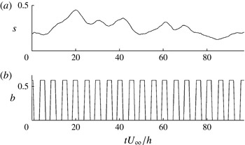
Figure 11(a) shows the reduction of the recirculation area using periodic forcing (figure 11
b). Control is effective in reducing the recirculation. The cost function for this control law is
 $J_{periodic}=0.423$
which is quite similar to the one found through genetic programming (
 $J_{genetic}=0.419$
). The MLC law still performs slightly better. Intriguingly, similar performances are achieved but with quite different dynamics and frequencies. The periodic forcing excites the Kelvin–Helmholtz frequencies at 1 Hz while the MLC law exploits the flapping frequency around 0.1 Hz.
(a) System response to periodic forcing over 100 convective time units. (b) Corresponding actuation.

4.4. Robustness
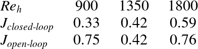
The control law was tested for various Reynolds numbers in order to test its robustness. Table 1 shows the resulting cost functions. The cost function does not increase by more than 20 % while Reynolds number changes by a factor 2. The cost function for the open-loop forcing is also shown. This open-loop forcing is done at the optimal shedding frequency at
 $\mathit{Re}_{h}=1350$
and is not changed with Reynolds number. Because it is tied to the recirculation area, MLC control law adapts to changes in operating conditions, ensuring consistent, reliable performance. Because natural frequency changes with free-stream velocity, the open-loop control shows poor performance at different Reynolds numbers. Performance variations for the MLC law are due to changes in jet to cross-flow momentum ratio. To further improve robustness the control law could be amended in the following way:
 $b=f(\mathit{Re}_{h})K(s)$
where
 $f$
is a function to be determined.
Cost function at different Reynolds numbers.

5. Conclusion
Machine learning control has been used to determine a cost-effective control law minimizing recirculation on a backward-facing step flow. During the twelve generations needed to converge towards the control law, the population has evolved toward solutions better fitting the problem, which is translated to lower cost function values. The process is stopped when no further amelioration can be foreseen, judging by the statistical values returned by the algorithm. As no convergence can be proven, there is no guarantee that this control is optimal. However, the nature of the cost function allows one to judge the performance of the solution and whether actuation can be rated as effective.
Without deriving a model for the input–output system, the genetic programming approach is able to converge on an efficient and robust control law linking a real-time measure of recirculation area to actuation value. Though the design of the experiment is kept at its simplest, an 80 % reduction of the recirculation area has been achieved. Moreover, the control law obtained highlights a mechanism which is not based on the exploitation of the Kelvin–Helmholtz instability as for the open-loop control, but rather on lower frequencies which are likely to be related with frequencies of the recirculation region.
Robustness can be increased by closed-loop laws. It is demonstrated that the control law designed by genetic programming for a given Reynolds number remains efficient in other operative conditions, compared to open-loop designed control which has rapidly deteriorating performance. Robustness would be reinforced by integrating a condition change during evaluation, though it would lengthen overall evaluation time.
Genetic programming has proven to be efficient at resolving multi-input/multi-output problems. Thus adding more freedom to the algorithm, by adding control outputs and sensors inputs, will increase the number of mechanisms the control laws can access in order to reduce the cost function. For instance adding time delays or derivative of the sensor would allow an embedding of the dynamical system and thus allow the control law to access more information on the state of the system.
This novel approach to experimental flow control competes with other approaches in terms of efficiency and robustness. Being model-free and capable of producing virtually any kind of control law (linear, nonlinear, with history of sensors and actuators) it can be used in a systematic fashion, with a known time consumption. This enables the method to be used on flows with a specific geometry which has not been thoroughly investigated, such as a detailed vehicle model or a turbine geometry.
Acknowledgements
N.G. and J.-L.A. wish to thank the DGA for their support, T.D. and B.R.N. acknowledge funding by the French ANR (Chaire d’Excellence TUCOROM and SEPACODE), M.S. and M.A. acknowledge the support of the LINC project (no. 289447) funded by ECs Marie-Curie ITN program (FP7-PEOPLE-2011-ITN).
Appendix A
In this appendix we provide further explanations about how control laws are translated from expression trees (§ A.1) and how the mutation and crossover operations are performed (§ A.2).
A.1. Control laws and expression trees
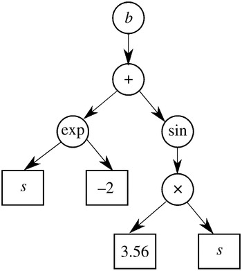
An expression-tree can be viewed in a graphical way as a tree-like representation of the function under consideration as in figure 12 with nodes (round shapes) representing user-defined functions and leaves (square shapes) representing the constants and inputs of the function. The root of the tree (the top node) is the function output. This tree can also be described by a LISP expression. A LISP expression is easily generated and manipulated from a computational point of view. For instance the function
 $b(s)=\exp (s-2)+(\sin (3.56\ast s))$
which is represented by the tree in figure 12 is represented by the LISP expression
 $+(\exp (+(-2s)(\sin (\ast 3.56s))))$
. The fact that the operator comes first allows one to generate, evaluate and manipulate the individual with recursive functions.
A typical expression tree.

A.2. Genetic programming operations on expression trees
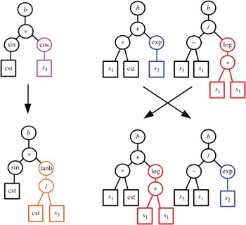
Figure 13 illustrates how the operations of mutation and crossover are performed.
(a) A possible mutation of an individual. (b) A possible crossover between two individuals.

The mutation operations (a) are performed by selecting a node, erasing the node and its subtree and growing a new subtree randomly. Part of the information contained in the individual is kept while new information is allowed to enter the population. The mutation operation increases the diversity and is responsible for exploring the search space with larger steps. The crossover operation (b) consists of selecting one node in each of the two individuals under consideration. The nodes and their subtrees are then exchanged. No new content is brought in but combinations of operations from good individuals (they have both won a seven-contestant tournament) are tested together. The crossover is responsible for exploring the search space around individuals that are performing correctly. By adjusting the crossover and mutation probabilities, it is possible to adjust the genetic programming way of converging. A high rate of mutation will explore more of the search space while a high rate of crossover will converge faster around detected minima, whether global or local.