

1. Introduction
Institutional quality is widely believed to be a fundamental determinant of income levels (Acemoglu et al., Reference Acemoglu, Johnson, Robinson, Aghion and Durlauf2005 and Helpman, Reference Helpman1998). This belief is supported by a wealth of cross-country empirical studies, several of which utilize the Fraser Institute's economic freedom scores as proxies for institutional quality.Footnote 1 These scores measure the extent to which ‘individuals are permitted to choose for themselves and engage in voluntary transactions as long as they do not harm the person or property of others’ (Gwartney et al., Reference Gwartney, Lawson and Hall2013: 1). They are proxies for institutions that are consistent with well-defined and enforced property rights, as well as for limited government in terms of both its size and scope.
The findings of cross-country empirical studies have largely been echoed by those using the analogous US state-level scores from the Fraser Institute's Economic Freedom of North America (EFNA) project (Stansel and McMahon, Reference Stansel and McMahon2013).Footnote 2 Furthermore, Stansel (Reference Stansel2013) has recently constructed US metropolitan area-level scores based on the EFNA methodology and, using these scores, reports a positive income-freedom correlation.Footnote 3 The positive correlation between 381 metropolitan area (log) per capita income levels and their freedom scores is illustrated in Figure 1. The left and right panels are based on, respectively, 2005 and 2011 income levels. However, both Stansel (Reference Stansel2013) and Figure 1 report only simple bivariate correlations. One of our goals here is to more carefully estimate the relationship between real per capita incomes (or their growth rates) and economic freedom in the US. We do this using Stansel's economic freedom scores for 381 metropolitan areas along with data on personal income and 25 additional control variables.
Real (log) per capita personal incomes and economic freedom scores for US metropolitan areas.

Another of our goals is to take advantage of the large number of US metropolitan areas and allow for spatial dependence in income levels and growth rates. Allowing for this possibility is important and interesting for at least two reasons. First, uncontrolled-for spatial dependence can result in inconsistent or otherwise biased estimates of the relationship between income and economic freedom (Corrado and Fingleton, Reference Corrado and Fingleton2012). Second, there are compelling reasons to believe that changes in one metropolitan area's institutional quality can impact the incomes of neighboring areas. These effects can operate through a variety of different channels, where some take immediate effect, while others may take longer to have an impact.
In the short run, for example, if a metropolitan area lowers its tax rates then this may increase its business activity in part by drawing customers away from businesses in neighboring areas. Alternatively, lower tax rates can lead to increases in disposable income that are partially spent at businesses in neighboring areas. In the longer run, we may see individuals and businesses relocating to metropolitan areas where there have been improvements in institutional quality, leading to higher incomes in the improved metropolitan areas and lower incomes elsewhere.Footnote 4 As shown in Ashby (Reference Ashby2007), states with higher levels of economic freedom experience greater migration inflows, suggesting that individuals base their location decisions partly on institutional quality. This effect will likely be stronger when looking at metropolitan areas, as it is often less costly for individuals to move smaller distances. However, another possibility is that the increased business activity in the improved metropolitan area may result in increased business activity in neighboring areas as well due to agglomeration effects. Taken together, we are interested in knowing the extent to which economic freedom-enhancing reforms are associated with positive-sum effects, or whether the effects are actually zero- or even negative-sum once spatial dependence is taken into account?
The spatial dependence that we allow for is in geographic space. This makes sense if the individuals, firms, and governments of geographic neighbors face lower transaction costs to trading with and learning from one another. A geographic definition of a metropolitan area's ‘neighbors’ also ensures that the weight matrix employed in our estimations is independent of the variation in our control variables (i.e., the weights are exogenous). Given our focus on geographic space, our paper is similar to Ahmad and Hall's (Reference Ahmad and Hall2012) study of the relationship between institutions and income growth across 58 countries, and also to Arbia et al. (Reference Arbia, Battisti and Di Vaio2010) study based on a sample of 271 NUTS-2 territorial units across 29 European countries.Footnote 5 However, neither set of authors calculate correct estimates of the direct, indirect, and total effects in the way described by LeSage and Pace (Reference LeSage and Pace2009). Doing so is important because, for any econometric model that includes a spatial lag of the dependent variable, the spillover and feedback effects make the interpretation of coefficients more complex than in the case of OLS.Footnote 6 We improve upon recent practice in the literature and report the correct direct, indirect, and total effects estimates as described by LeSage and Pace (Reference LeSage and Pace2009).
An informal look at the data suggests there are indeed positive-sum games that operate across metropolitan areas in geographic space. For example, looking only within California we see that areas that have lower economic freedom levels, based on the Stansel (Reference Stansel2013) index, yet are close to areas with higher economic freedom levels, have higher income levels than more isolated areas with similar levels of economic freedom. More specifically, the Los Angeles-Long Beach metropolitan area is much less economically free than the nearby metropolitan area of Santa Ana–Anaheim–Irvine, and therefore has a per capita income level that is much lower. However, the Los Angeles-Long Beach metropolitan area has a much higher income level than other California metropolitan areas with nearly identical levels of economic freedom, yet is more isolated from areas that have high levels of economic freedom (namely, Yuba City and Redding). A primary aim of this paper is to provide a more formal analysis of these potential spatial relationships.
We report that the estimated direct and total effects of economic freedom on metropolitan area income levels are positive over both a 3-year and 9-year horizon. In addition, when we examine growth rates, we find that economic freedom has a positive total effect on per capita income growth rates over both horizons. Over 3 years the direct effect of economic freedom is positive while the indirect effect is statistically insignificant. Alternatively, over 9 years the indirect effect of economic freedom is positive while the direct effect is insignificant. We interpret this as indicating the diffusion of growth effects over time. In all cases (levels or growth rates; 3-year or 9-year horizon) the point estimates of the statistically significant total effects are greater than those of the direct effects. Overall, then, the evidence strongly suggests that economic freedom-enhancing reforms in a metropolitan area yield positive-sum interactions with neighboring areas.
We organize this paper as follows. In Section 2, we describe the data with particular attention given to Stansel's (Reference Stansel2013) economic freedom index. In Section 3, we explain our choice of empirical models and estimation method. We report and discuss our results in Section 4. Then we offer some summary conclusions and comments in Section 5.
2. Data
The control variable of interest is the Stansel (Reference Stansel2013) economic freedom index. An index value is available for each of the 384 US metropolitan areas for the year 2002. The index is designed to provide a comprehensive measure of the extent to which private property is protected from expropriation and individuals are allowed to engage in voluntary transactions.
The index is constructed on a scale from 0 to 10, with 10 indicating most free. The comprehensive index is an average of the scores that metropolitan areas receive for three areas of economic freedom separately (each also on a scale of 0 to 10). Each area of economic freedom is itself scored based on a number of related components:
• Area 1: Size of Government: (a) government consumption expenditures by government; (b) transfers and subsidies; (c) social security payments.
• Area 2: Takings and Discriminatory Taxation: (a) total tax revenue; (b) individual income tax revenue; (c) indirect tax revenue; (d) sales taxes collected.
• Area 3: Labor Market Freedom: (a) minimum wage annual income; (b) state and local government employment; (c) union density.Footnote 7
Most of the components listed above are in dollar terms and are taken as a percentage of metropolitan area personal incomes. Government employment is taken as a percentage of total employment, as are union employees to arrive at a measure of union density.
The 384 metropolitan areas include 355 metropolitan statistical areas (MSAs) and 29 metropolitan divisions (MDs). These MSAs and MDs are defined according to the 2009 Office of Budget and Management definitions. The 29 MDs are portions of 11 large MSAs that Stansel breaks down so that all of the metropolitan areas are of comparable sizes. Since we are pursuing a spatial econometric analysis, we limit ourselves to the 381 metropolitan areas of the contiguous US states (i.e., Alaska and Hawaii areas are excluded). As can be seen in Figure 2, there is considerable variation in the economic freedom scores across US metropolitan areas. Figure 2 also seems to suggest that levels of economic freedom are similar across neighboring metropolitan areas. This would be consistent with yardstick competition playing an important role in determining institutional quality and resulting in spatial correlation in economic freedom scores. Casual inspection suggests that the spatial correlation is not entirely accounted for by intra-state similarities. All else equal, then, economic freedom scores may be converging across metropolitan areas over time. However, as our data only contain metropolitan area freedom index values for one year, 2002, we cannot provide more systematic evidence for or against such convergence.Footnote 8 Even so, the idea of yardstick competition is important to keep in mind while interpreting the results.
Economic freedom scores for US metropolitan areas.
Our dependent variable will be metropolitan area real (log) personal per capita income, or its average annual rate of growth. We use the US Bureau of Economic Analysis's (BEA’s) measure of personal income. The BEA's measure of personal income includes transfer payments. Since we are only interested in the income individuals receive from production, we net out the BEA's estimate of transfer payments for each metropolitan area.
Institutions and their effects on incomes are persistent. In lieu of a well-defined time frame for those effects, we consider income levels in 2005 and also in 2011 (or the rate of growth over 2002–2005 and also over 2002–2011). We will often refer to results in terms of those ‘over the 3-year horizon’ or ‘over the 9-year horizon’ and, when we do so, we are referring to those where the dependent variable is based on, respectively, the 2005 or 2011 income level. In growth rate regressions, we also include 2002 personal income per capita as an initial income level control (to account for convergence effects). Personal income is always converted into 2005 constant dollars.Footnote 9 As in the case of economic freedom scores, per capita income levels appear to be spatially correlated across metropolitan areas (Figure 3; 2011 income levels); as do also their growth rates (Figure 4; 2002–2011 income growth rates).
Personal income per capita by metropolitan area in 2011.
Personal income per capita average growth rate from 2002–2011 by metropolitan area
We also employed 25 control variables that are motivated by Higgins et al. (Reference Higgins, Levy and Young2006) and Young et al. (Reference Young, Higgins and Levy2010, Reference Young and Levy2013) county-level studies of income growth. These data are all from either the US Census Bureau or the BEA.Footnote 10 The control variables include (i) a number of industry employment shares; (ii) three different educational attainment population shares (high school diploma, some college, and bachelor's degree or higher); and (iii) a number of demographic population shares (e.g., age and racial demographics).Footnote 11 We also control for a metropolitan area's land and water areas per capita. All estimations include state-level fixed effects to account for unobserved characteristics at that level.Footnote 12 The data for (i), (ii), and (iii) are all based on either the year 2000 or the year 2002.
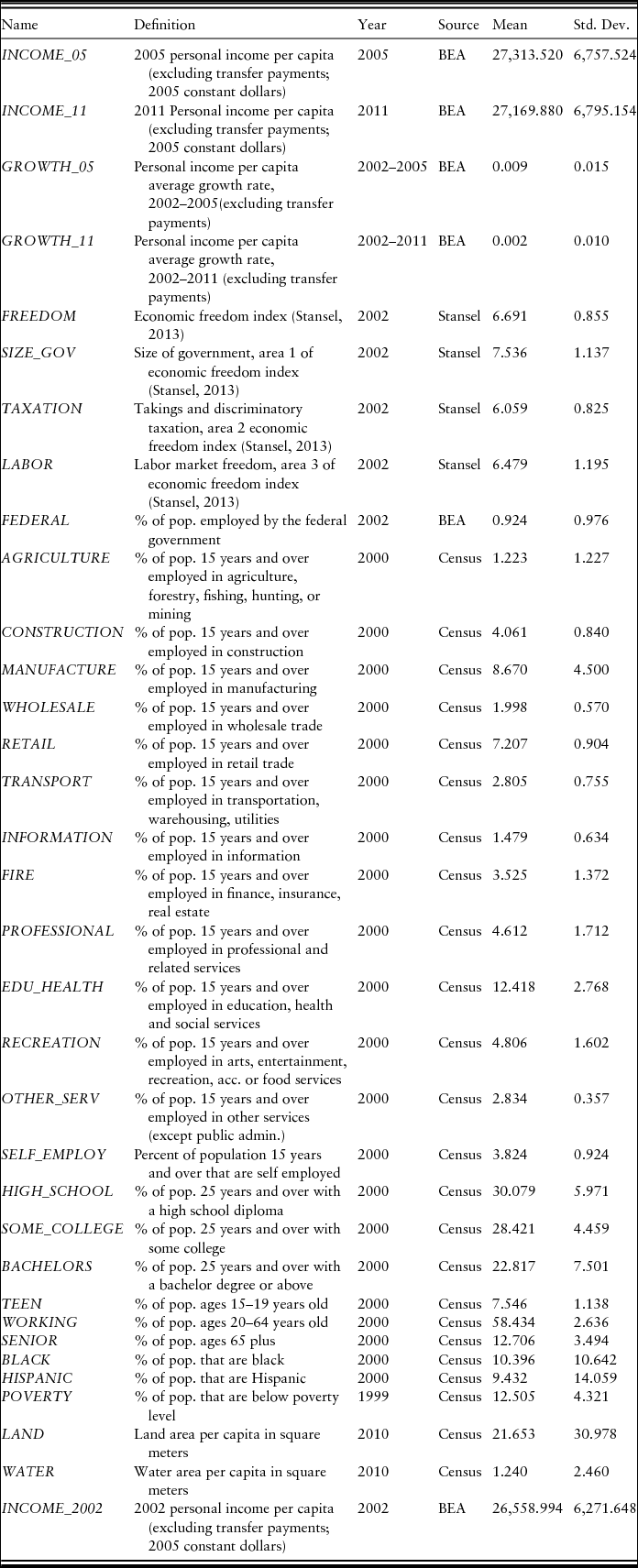
Definitions, years, and sources for all variables are reported in Table 1, along with summary statistics.
Variable definitions, sources, and summary statistics
3. Empirical methodology and model choice
Our dependent variable is either a metropolitan area's (log) real per capita income level or its average annual growth rate. We relate this to, among other controls, a metropolitan area's economic freedom score from Stansel (Reference Stansel2013). We employ Elhorst's (Reference Elhorst2010) testing procedure to determine whether there is spatial dependence in our data and, if there is, what is the appropriate spatial econometric model for our analysis.
In addition to (1) OLS, the Elhorst testing procedure evaluates four spatial models: (2) the spatial autoregressive model (SAR), (3) the spatial error model (SEM), (4) the spatial lag of X model (SLX), and (5) the spatial Durbin model (SDM). A general form that nests each of these alternative models is
 \begin{equation}
y = \alpha + \rho Wy + X\beta + WX\theta + \varepsilon ;\end{equation}
 \begin{equation}
\varepsilon = \lambda W\varepsilon + \upsilon ,\end{equation}
where y is an n × 1 vector of cross-sectional observations on the dependent variable; X is an n × m matrix of control variables weighted by the m × 1 vector of coefficients, β; and ɛ is an n × 1 vector of errors.Footnote 13 In equations (3.1) and (3.2), W is an n × n weight matrix that defines neighbor relations, ρ and λ are scalar parameters, and θ is a k × 1 vector of parameters (where k is the number of X variables) defining spatial effects across neighbors. In the simplest case, if ρ, θ, and λ are all zero then we are left with a standard OLS model. Alternatively, spatial dependence can exist in the dependent variable (y), the independent variables (X), or the error term (ɛ). Each of the specific models (1) through (5) can be arrived at through parameter restrictions on the general model (3.1) and (3.2):
• OLS: ρ = θ = λ = 0;
• SAR: θ = λ = 0;
• SEM: ρ = θ = 0;
• SLX: ρ = λ = 0;
• SDM: λ = 0.
As LeSage and Pace (Reference LeSage and Pace2009) explain, given that the true data generating process is uncertain, in the presence of spatial dependence the SDM model, (5), is the most likely model to produce unbiased estimates since it is actually a generalization of models (1) through (4).Footnote 14 Consequently, SDM is likely to be the appropriate model unless testing provides statistically significant evidence to the contrary. The Elhorst (Reference Elhorst2010) testing procedure systematically searches for such evidence.
To test for spatial dependence we first need to specify the weight matrix, W. We define neighbor relations according to a ‘k-nearest-neighbors’ criterion. Since US metropolitan areas have on average six contiguous neighboring areas, a reasonable assumption is k = 6. We therefore define a metropolitan area's neighbors as the six other metropolitan areas that are closest to the center of its geographic mass.Footnote 15 Based on the six closest neighbors, entries in the W matrix are assigned 1s to indicate metropolitan area neighbor pairs. All of the other elements of W are assigned 0s. Following convention we ‘row normalize’ the entries such that the rows of the W matrix all sum to one.Footnote 16 While k = 6 is reasonable, it is also to some extent arbitrary. However, for spatial models that include a ρ parameter, as long as the estimates are interpreted properly they will not be sensitive to this particular choice of k (LeSage and Pace, Reference LeSage and Pace2014).
With W specified as described above, we begin the Elhorst (Reference Elhorst2010) testing procedure by conducting Lagrange multiplier (LM) tests to determine if there is any spatial dependence in our data. Specifically, we estimate the OLS model and test the hypothesis of no spatial dependence in the dependent variable (SAR) using an LM lag test; then we test the hypothesis of no spatial dependence in the error term (SEM) using the LM error test. The appeal of these tests is that they only require the residuals of the OLS estimation and W. A drawback of both of the LM tests is that the specific sources of spatial dependence can sometimes be hard to distinguish from one another (i.e., each of the standard LM tests has power over the alternative form of spatial dependence). We employ robust versions of these LM tests that take this into account.
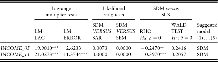
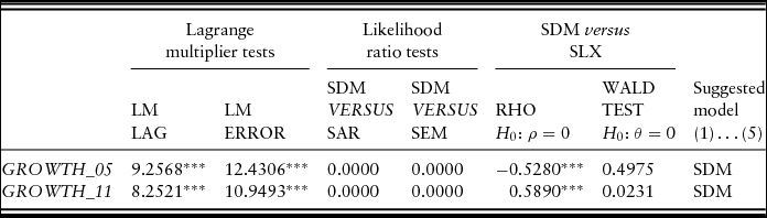
Tables 2 and 3 report the results of these LM tests for per capita income levels (INCOME_05 and INCOME_11) and average growth rates (GROWTH_05 and GROWTH_11), respectively. The levels are for 2005 or 2011; the average growth rates are for 2002–2005 or 2002–2011. The results are uniform. The LM tests always reject the null hypothesis of no spatial dependence in the OLS model, suggesting that we have spatial dependence in the dependent variable, the error term, or both.
Model specification tests: per capita income levels
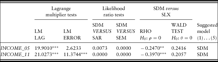
Notes: Table gives LM value for the LM lag and LM error tests, p value for likelihood ratio tests and WALD tests, and estimated coefficient for RHO in the SDM. *** indicates statistically significant at 1% level, ** indicates statistically significant at 5% level, * indicates statistically significant at 10% level.
Model specification tests: average per capita income growth rates
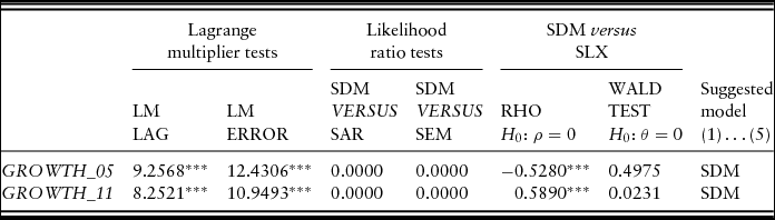
Notes: Table gives LM value for the LM lag and LM error tests, p value for Likelihood Ratio tests and WALD tests, and estimated coefficient for RHO in the SDM. *** indicates statistically significant at 1% level, ** indicates statistically significant at 5% level, * indicates statistically significant at 10% level.
Having rejected the null hypothesis of no spatial dependence for both income levels and growth rates, the next step of the procedure is to estimate the SDM model to determine if the spatial dependence is more general than either the SAR or the SEM models allow for. We use the estimate of the SDM model to conduct a likelihood ratio (LR) test to determine if SDM is more appropriate than either SAR or SEM. If SDM is found to be more appropriate than the SAR and SEM models, we then also need to test if the ρ parameter in the SDM model is statistically significant once we allow for spatial dependence in the explanatory variables. Specifically, we first test the following two hypotheses: H0: θ = 0 and H0: θ + ρβ = 0, where θ, β, and ρ are as defined in equation (3.1). The first hypothesis is that the SDM model can be collapsed into the SAR model, while the second hypothesis is that SDM model can be collapsed into the SEM model. If both hypotheses are rejected, then we accept that the SDM is more appropriate than both the SAR and SEM models. If H0: θ = 0 is not rejected then we employ the SAR model as long as the robust LM tests point to SAR. Similarly, if H0: θ + ρβ = 0 is not rejected then we employ the SEM model as long as the robust LM tests point to SEM. If either of these conditions is not satisfied then the SDM model is employed by default.
Furthermore, if we deem SDM more appropriate than either SAR or SEM, or both, we need to test if ρ is statistically different from zero in the SDM model as we are now allowing for spatial dependence in the explanatory variables. If we cannot reject the null hypothesis that ρ is statistically different from zero, we then need to re-estimate OLS including spatially lagged explanatory variables, with no spatially lagged dependent variable, i.e., the SLX model. This SLX estimate would be used to test the hypothesis H0: θ = 0; i.e., if the spatially lagged explanatory variables are collectively statistically different from zero. If this hypothesis cannot be rejected, we still use the SDM model since we found the spatial dependence in the data to be more general than the SAR or SEM models allow.
The results from this testing procedure are reported in Tables 2 and 3 for, respectively, income levels and growth rates. In all cases, the hypotheses that SDM can be collapsed into either the SAR or SEM models area rejected. Furthermore, the estimate of ρ is statistically different from zero in all cases. Notice, that according to the Wald test, θ is not statistically different from zero in any case for the income levels (Table 2) and only for one case for the growth rates (Table 3). However, even with this finding, according to the testing procedure SDM is the most appropriate model for all specifications. This is because we have already found that the spatial dependence is more general than a simple SAR model would allow. SDM results are estimated using maximum likelihood. Maximum likelihood avoids the simultaneity bias that would arise in an OLS estimation that includes a spatially lagged dependent variable.
4. Results
We begin by reporting OLS estimations (not allowing for spatial dependence) using metropolitan area (log) per capita income levels or average growth rates as the dependent variables. To our knowledge, the present study is the first to estimate the relationship between economic freedom and income across US metropolitan areas while controlling for a large number of economic and demographic variables, as well as state-level fixed effects. The OLS results then, both serve as useful benchmark and may be interesting in their own right. We then report estimations of spatial econometric models. Based on the results of Elhorst (Reference Elhorst2010) specification tests we estimate SDM models using both the 2005 and 2011 income levels as dependent variables; also SDM models using both the 2002–2005 and 2002–2011 annual growth rates as dependent variables. In the growth rate estimations, we include the initial (2002) (log) per capita income level as an additional control. Otherwise the control variable set is the same across the four spatial econometric estimations. (See Section 2 above and Table 1 for details on the control variable set.)
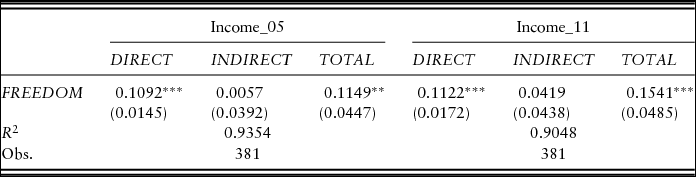
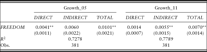
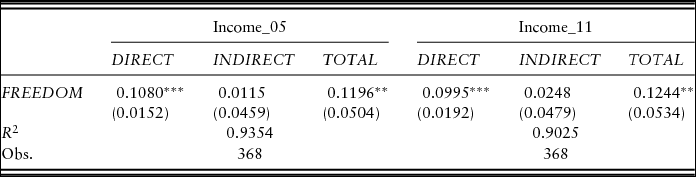
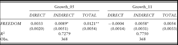
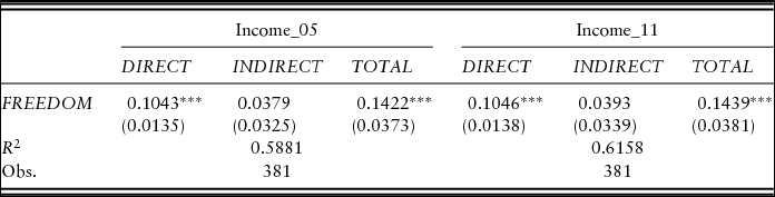
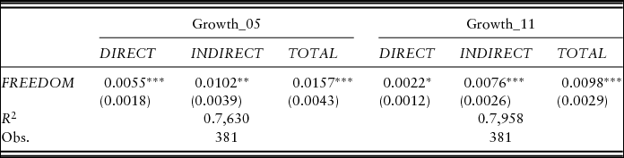
To conserve space Tables 4–12 report only the estimated direct, indirect, and total effects associated with a metropolitan area's 2002 economic freedom score (FREEDOM), along with the R2 of each estimation. However, full estimation results are found in Table A1, through Table A9 of an online appendix.Footnote 17
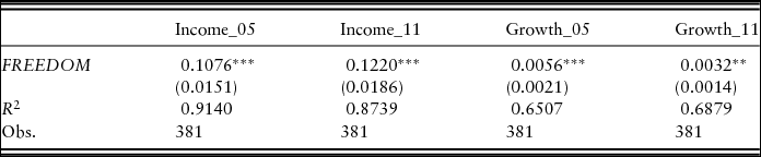
OLS effect estimates of economic freedom on metropolitan area per capita income levels
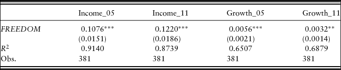
Notes: *** indicates statistically significant at 1% level, ** indicates statistically significant at 5% level, * indicates statistically significant at 10% level. Standard errors are in parentheses. Full set of controls, constant, and state fixed effects included in all regressions. All growth rate regressions include INCOME_2002 as an additional control.
SDM direct, indirect, and total effect estimates of economic freedom on metropolitan area per capita incomes
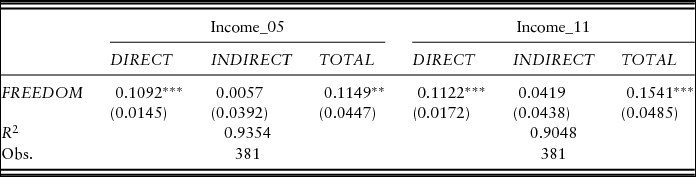
Notes: *** indicates statistically significant at 1% level, ** indicates statistically significant at 5% level, * indicates statistically significant at 10% level. Standard errors are in parentheses. Full set of controls, constant, and state fixed effects included in all regressions.
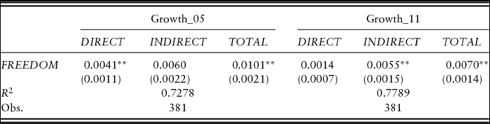
SDM direct, indirect, and total effect estimates of economic freedom on metropolitan area per capita income growth rates
Notes: ***indicates statistically significant at 1% level, **indicates statistically significant at 5% level, *indicates statistically significant at 10% level. Standard errors are in parentheses. Full set of controls, constant, and state fixed effects included in all regressions. All growth rate regressions include INCOME_2002 as an additional control.
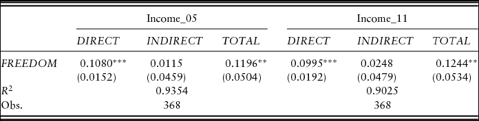
SDM direct, indirect, and total, effect estimates of economic freedom on metropolitan area per capita incomes excluding observations with an economic freedom score further than two standard deviations from the mean
Notes: ***indicates statistically significant at 1% level, **indicates statistically significant at 5% level, *indicates statistically significant at 10% level. Standard errors are in parentheses. Full set of controls, constant, and state fixed effects included in all regressions.
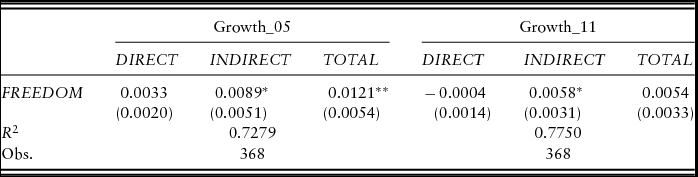
SDM direct, indirect, and total, effect estimates of economic freedom on metropolitan area per capita income growth rates excluding observations with an economic freedom score further than two standard deviations from the mean
Notes: ***indicates statistically significant at 1% level, **indicates statistically significant at 5% level, *indicates statistically significant at 10% level. Standard errors are in parentheses. Full set of controls, constant, and state fixed effects included in all regressions. All growth rate regressions include INCOME_2002 as an additional control.
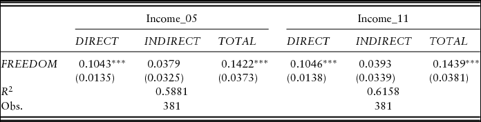
SDM direct, indirect, and total, effect estimates of economic freedom on metropolitan area per capita incomes using a contiguous weight matrix
Notes: ***indicates statistically significant at 1% level, **indicates statistically significant at 5% level, *indicates statistically significant at 10% level. Standard errors are in parentheses. Full set of controls, constant, and state fixed effects included in all regressions.
SDM direct, indirect, and total, effect estimates of economic freedom on metropolitan area per capita income growth rates using a contiguous weight matrix
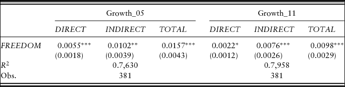
Notes: ***indicates statistically significant at 1% level, **indicates statistically significant at 5% level, *indicates statistically significant at 10% level. Standard errors are in parentheses. Full set of controls, constant, and state fixed effects included in all regressions. All growth rate regressions include INCOME_2002 as an additional control.
SDM direct, indirect, and total, effect estimates of each area of economic freedom on metropolitan area per capita incomes
Notes: ***indicates statistically significant at 1% level, **indicates statistically significant at 5% level, *indicates statistically significant at 10% level. Standard errors are in parentheses. Full set of controls, constant, and state fixed effects included in all regressions.
SDM direct, indirect, and total, effect estimates of each area of economic freedom on metropolitan area per capita income growth rates
Notes: ***indicates statistically significant at 1% level, **indicates statistically significant at 5% level, *indicates statistically significant at 10% level. Standard errors are in parentheses. Full set of controls, constant, and state fixed effects included in all regressions. All growth rate regressions include INCOME_2002 as an additional control.
Main results
The benchmark (no spatial dependence) OLS results are reported in Table 4. In all cases, we find that an increase in a metropolitan area's 2002 freedom score is associated with a statistically significant (5% level or better) increase in per capita income levels and growth rates. This is consistent with the previous literature based on US state-level and cross-country level economic freedom scores. However, the evidence reported in Section 3 strongly suggests that spatial dependence is present in our data. If spatial dependence is present and not controlled for then the benchmark OLS estimates are likely to be biased. Furthermore, we are interested in knowing not only the direct effects of a metropolitan area's economic freedom on its income, but also the indirect effects on its neighbors’ incomes.Footnote 18
Results based on the estimation of SDM income level models are reported in Table 5. Recall that since the SDM model assumes spatial dependence in the dependent variable (the ρ parameter from equation (3.1)), there are feedback effects that make the interpretation of coefficient estimates less straightforward than in the case of the OLS model without spatial dependence. Therefore, we compute correct estimates of the direct, indirect, and total effects as described by LeSage and Pace (Reference LeSage and Pace2009). It is important to note that these indirect and total effects estimates represent cumulative effects, not effects per neighbor. In other words, these effects represent changes in the dependent variable across all surrounding areas resulting from a change in the level of economic freedom in a single area. Thus, the total (direct plus indirect) effect will most likely be significantly larger than the direct effect if economic freedom exhibits positive spillovers.
Based on the LeSage and Pace (Reference LeSage and Pace2009) estimates, an increase in a metropolitan area's 2002 freedom score is associated with a statistically significant (1% level) increase in its own per capita income level in 2005. The same is true based on 2011 income levels and the coefficient point estimates are very similar (0.1092 versus 0.1122). In other words, a 1 point increase in FREEDOM is associated with, all else equal, a direct and positive effect on a metropolitan area's per capita income level of around 11%. (A standard deviation increase in FREEDOM is 0.855, so its analogous direct effect on income levels is about 9.4%.) Furthermore, the estimated indirect effects that occur through neighbor relations are positive although statistically insignificant. The total effects (direct plus indirect) of an increase in economic freedom are both positive and statistically significant (at least 5% level), and the point estimates are larger than the direct effects: 0.1149 and 0.1541 over the 3-year and 9-year horizons respectively. (However, consistent with the indirect effects being statistically insignificant, the 95% confidence intervals contain the direct effect point estimates.) We also note that the SDM models account for the largest part of the variation in the dependent variables. (The R2s are both greater than 0.90.)
The results reported in Table 5 suggest that a 1 point increase in a metropolitan area's economic freedom score is associated with not only an increase in its own per capita income of about 11%, but also a cumulative increase – including the effects, a metropolitan area has on per capita incomes of neighboring metropolitan areas – that is at least as large. The point estimates indicate the increase to be approximately 12–15%. Over the 3-year horizon, a 12% increase in income is equal to about $3,227, using the mean of INCOME_05 as the benchmark. Thus, a 1 point increase in a metropolitan area's economic freedom score explains only 48% of a standard deviation change in INCOME_05, on average. While the effects over the 9-year horizon are slightly larger in magnitude, a 1 point increase in a metropolitan area's economic freedom score explains only 59% of a standard deviation change in INCOME_11, on average.
However, despite the standard deviation of FREEDOM being less than 1 point, considerable differences in economic freedom exist across prominent metropolitan areas. To put a 1 point change in the freedom score in some perspective, the difference between the San Francisco–San Mateo–Redwood City metropolitan area (6.70) and the New York–White Plains–Wayne metropolitan area (4.60) is over 2 points; and the difference between the Dallas–Plano–Irving (7.86) area and the New York–White Plains–Wayne area is over 3 points. Total effects of 12–15% associated with a 1 point change constitute, then, economically large effects across some prominent metropolitan areas.
Changes in FREEDOM are also positively related to economic growth. Table 6 reports the SDM model results where average income growth rates (from 2002–2005 and 2002–2011, respectively) are the dependent variables. In both cases, the total effect is statistically significant (5% level) and positive. More specifically, a 1 point increase in the freedom index is associated with about a 1 % point cumulative increase in the growth rates throughout all areas over the 3-year horizon, and about a 0.7 % point increase over the 9-year horizon. While both total growth effects are positive and significant, an interesting pattern emerges moving from the direct and indirect effects at the 3-year horizon to those over the 9-year horizon. The estimated direct effect over the 3-year horizon is positive and statistically significant (5% level). However, the direct effect is not statistically significant over the 9-year horizon and the point estimate is much smaller (0.0014 versus 0.0041). Alternatively, the indirect effect is only statistically significant over the 9-year horizon (point estimate equal to 0.0055). A plausible interpretation of this pattern is that it reflects the impact of a change in economic freedom and its spillovers throughout time. Over the shorter horizon, the statistically significant effects are those occurring directly to the metropolitan area where a change in freedom occurs; over the longer horizon, the indirect effects on neighboring areas become more important.
Focusing on the total effects, a 1 point increase in a metropolitan area's economic freedom score is associated with between a 0.7 and 1 % point cumulative increase in growth rates. The mean 2002–2011 metropolitan area growth rate in our sample is about 0.2 %, so the total effect is between 3.5 and 5 times the growth rate of the average metropolitan area. If we use the 2002–2005 mean growth rate of 0.9% (which may be more meaningful because 2002–2005 excludes the Great Recession) the total effect is just about as large as that mean growth rate. Another meaningful benchmark is 2%, which is widely thought to be approximately the long-run balanced growth rate for developed economies. The estimated total (cumulative) effect on metropolitan area growth rates of a 1 point increase in the economic freedom score of a given metropolitan area is between 35% and 50% of that long-run benchmark. From any of these perspectives, the estimated total effects are economically meaningful.
The results of Table 6 are interesting in that the total effects of economic freedom on growth rates seem to dissipate over time, while the total effects of economic freedom on income levels (Table 5) seem to become larger over time. This makes sense given the cumulative impact on income levels that temporary increases growth rates will have. Also, note that much of the increase in the magnitude of the total effect on income levels occurs because of an increase in the indirect effect moving from the 5-year horizon to the 11-year horizon. (This statement is based on the point estimates, even though the 11-year indirect effect on levels is not statistically significant.) Taken together the results from Tables 5 and 6 suggest that an increase in a metropolitan area's economic freedom level has a large and positive, though temporary, effect on its income growth rate in the near term. There are also positive spillovers to neighboring area growth rates that play out during and subsequent to the direct effect, though they are ultimately also temporary. These spillovers are relatively small per neighbor but, over the 11-year horizon, cumulatively comparable to (and by the point estimate larger than) the direct growth rate effect. This pattern is consistent with both a total growth rate effect that dissipates moving from the 5-year horizon to the 11-year horizon, as well as a total effect on income levels that increases from the one horizon to the next.
Robustness checks
In an illustrative example above we noted that, while the standard deviation of FREEDOM in our sample is 0.855, finding considerably larger differences in scores across widely-recognizable counties is not difficult. For example, the 2.1 point difference between the San Francisco–San Mateo–Redwood City metropolitan area (6.70) and the New York–White Plains–Wayne metropolitan area (4.60); likewise the 3.26 point difference between the Dallas–Plano–Irving (7.86) area and the New York–White Plains–Wayne. This may raise concerns that our results are being driven primarily by a small number of exceedingly free or unfree outlier areas. To check this, Tables 7 and 8 report SDM results for income levels and growth rates, respectively, when we exclude metropolitan areas with an economic freedom score more than plus or minus 2 standard deviations from the 6.691 mean.
The level results in Table 7 are qualitatively and also, for the most part, quantitatively unchanged from those reported in Table 5. (The most notable change is that the point estimate for the INCOME_11 total effect falls from 0.1541 to 0.1244, but the two estimates are not statistically different from one another.) Alternatively, the results reported for growth rates in Table 8 are in some ways meaningfully different than those reported in Table 6. While all statistically significant results are still positive, we find that the indirect effect (as opposed to the direct effect in Table 6) is statistically significant over the 3-year horizon. Furthermore, the total effect over the 9-year horizon is no longer statistically significant. One interpretation of the different results contained in Table 8vis-à-vis Table 6 is that only large (relative to the sample variation) changes in economic freedom yield significant growth effects over sustained periods of time.Footnote 19
We also report a robustness check on whether the results are sensitive to our six closest neighbor weight matrix specification. LeSage and Pace (Reference LeSage and Pace2014) argue that the marginal effects are not sensitive to the choice of spatial weight matrix as long as the proper direct, indirect, and total marginal effects are calculated. However, we explore an alternative weighting scheme where neighbor relations are based only on contiguous relationships. Defining metropolitan areas as neighbors only if they share a border excludes cases where one (or more) of the six closest neighbors is extremely far away (e.g., metropolitan areas in Montana). The results reported using this alternative matrix are contained in Tables 9 and 10 for income levels and growth rates, respectively. They are very similar to those contained in Tables 5 and 6. Economic freedom has positive and statistically significant direct and total effects on both income levels and growth rates. The only difference is that, in the case of growth rates, the indirect (positive) effects of economic freedom are now also statistically significant (Table 10).
Individual freedom score areas
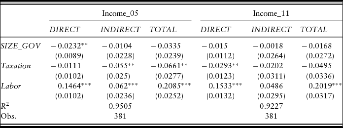
To get a better idea as to which areas of economic freedom are related to capita income levels and growth rates, Tables 11 and 12 report the results when the freedom index is disaggregated into its three constituent area indices. The LABOR market freedom area appears to be driving the positive relationship between economic freedom and income levels (Table 11). The direct and total estimated effects are positive and statistically significant at the 1% level over both the 3-year and 9-year horizons. The effects associated with labor market freedom are large enough to offset the negative relationships between income levels and both SIZE_GOV and TAXATION. (Recall that higher values of SIZE_GOV and TAXATION correspond to smaller government and lower taxes.) Over the 3-year horizon, the size of government area has a negative and significant (5% level) direct effect, even though its total effect is not statistically different than 0. In the case of takings and discriminatory taxation, the indirect and total effects are both negative and significant (5% level). Over the 9-year horizon, however, neither the SIZE_GOV nor TAXATION total effect is statistically different from 0. Notably, over either the 3-year or 9-year horizon, the total effects associated with SIZE_GOV and TAXATION are both in absolute value less than 32% as large as the LABOR total effect.
The results of Table 11 suggest that labor markets with less government interference and less powerful unions are associated with higher income levels; furthermore, this is true not only for the metropolitan areas where labor market freedom is greater, but also for neighboring areas. Alternatively, the effects associated with lower taxes, government expenditures, and transfers are smaller and more difficult to interpret. In terms of categorizing these effects as ‘smaller’, comparing the quantitative importance of changes in different indices must be done cautiously. In this case, the sample standard deviations of SIZE_GOV, TAXATION, and LABOR lie in the narrow range of 0.825 to 1.195, making the comparison of the point estimates reasonable.
TAXATION and SIZE_GOV may also be more difficult to interpret as both of these factors may change in response to changes in income. For example, when income falls, we may see governments responding by lowering the tax rate, thereby increasing TAXATION. However, the results also show that when income falls, government size also falls, thereby increasing SIZE_GOV. This is suggesting that these governments may be engaging in countercyclical policy when it comes to taxes, and pro-cyclical policy when it comes to government spending. It could also be the case that the negative relationship between SIZE_GOV and INCOME is the result of past countercyclical policy that turned out to be successful. Regardless of being pro-cyclical or countercyclical, if a local government's policy depends on the current condition of the economy, we may expect that these effects will dissipate over the long run as they do in Table 11.
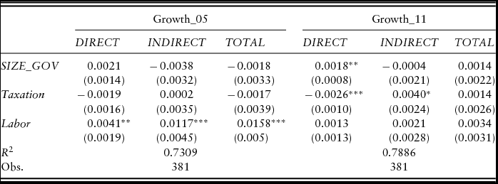
Regarding growth rates (Table 12), over the 3-year horizon labor market freedom is associated with positive and significant (5% level or better) direct, indirect, and total effects. Over the 9-year horizon, none of the individual area indices are associated with statistically significant total effects. For SIZE_GOV the direct effect is positive and significant (5% level); for TAXATION the direct effect is negative and significant but the indirect effect is marginally significant (10% level) and positive. These results contrast to those reported in Table 10 where, over the 9-year horizon, the direct, indirect, and total effects estimates associated with the comprehensive freedom index are all positive and statistically significant. One interpretation of this contrast is that we should accept Hall and Lawson's (Reference Hall and Lawson2014: 6) view that, when it comes to the concept of economic freedom, ‘the whole is greater than the sum of its parts’. In other words, the various dimensions of economic freedom measured by the sub-indices are complementary to one another. In addition, it is likely that each of category of economic freedom is highly correlated with the others, thus making separating their effects in a regression extremely difficult. As described in Lawson (Reference Lawson2006), breaking the economic freedom index up into its components often results in meaningless regression coefficients simply because of a high degree of collinearity. Therefore, for both reasons, we would expect FREEDOM (which is the average of LABOR, SIZE_GOV, and TAXATION) to be a more important determinant of income levels and growth rates than the individual areas taken separately.
Summary
The results reported above suggest two important conclusions. First, in the short- to even medium-run institutional reforms in metropolitan areas have positive spillovers to neighboring areas, causing the total effects on income to be larger than the direct effects. Second, given the potential spillovers, OLS results are likely underestimating the positive effects of freedom-enhancing reforms. The benchmark OLS growth and income effects are positive and statistically significant effect (at least at the 5% level; Table 4), but the point estimates are uniformly smaller than those for the total effects reported based on the SDM model (Tables 5 and 6). That being said, the SDM total effects estimates are not statistically different than those based on OLS.
It is important to note that the OLS point estimates bear no straightforward relationship to either the SDM direct effects or total effects point estimates. The OLS results cannot simply be interpreted as the correct effects conditional on neglecting spillovers. Rather, in the presence of spatial dependence the OLS estimates are biased and inconsistent. They can only be interpreted as non-casual partial correlations in the data. However, those partial correlations are still in and of themselves interesting given that our paper is the first to examine the relationship between economic freedom and income at the metropolitan area level while taking into account a large set of control variables, including state fixed effects.
5. Conclusions
A substantial empirical literature reports that economic freedom is an important determinant of both income levels and their rates of growth. These findings seem to hold when looking both across countries and within countries. In particular, several studies focusing on the US utilize the state-level EFNA scores to examine this relationship. Stansel (Reference Stansel2013) has recently developed a US metropolitan area-level economic freedom index based on the EFNA methodology. We utilize this new index to re-explore the relationships between economic freedom and both income levels and growth rates.
The Stansel (Reference Stansel2013) index allows us to contribute to the existing literature in at least two ways. First, given the large number of metropolitan areas in the US (381 in our analysis) we are able to carefully examine these relationships while including 25 additional control variables in the analysis, as well as state-level fixed effects. Second, the previous literature largely ignores the possibility of spatial dependence. Across the US, the movement of both labor and capital are relatively cheap; it is also relatively cheap to consumers to move their purchasing activities. Resource flows in response to institutional forms are likely to be an important part of the story. We are interested in knowing whether freedom-increasing reforms are associated with positive-sum gains; or whether those effects are actually zero- or even negative-sum once spatial effects are taken into account.
The results of this paper suggest at least two important conclusions. First, the gains to institutional reforms are not confined to the metropolitan area in which the reforms are enacted. We find statistically significant positive spillovers to incomes in neighboring metropolitan areas. Second, due to the presence of spatial dependence in this context OLS will likely lead to biased estimates of the relationships between economic freedom and economic outcomes.
Based on our SDM estimates, a 1 point increase in a metropolitan area's economic freedom score is associated with a positive direct effect on its per capita income level of about 11%. Taking into account spillovers, however, we estimate the total effect over a 9-year horizon to be an increase of about 15%. When we focus on income growth rates rather than levels, we find that the total effect associated with a 1 point increase in a metropolitan area's freedom score is about 1 % point increase in the growth rate over a 3-year horizon, and a 0.7 % point increase over a 9-year horizon. Interestingly, these total effects are driven by a statistically significant direct effect over the 3-year horizon and a statistically significant indirect effect over the 9-year horizon. A plausible interpretation of this pattern is that, over the shorter horizon, freedom-enhancing reforms will primarily affect growth in the metropolitan area in which they occur; however, as time passes, the growth effects of those reforms spillover to neighboring countries.
Acknowledgements
For helpful comments and discussion we thank Greg Randolph and other participants at the 2013 Southern Economic Association meetings in Tampa, FL; Todd Nesbit, Dean Stansel, and other participants at the 2014 Public Choice Meetings in Charleston, SC. Justin Ross read a previous draft closely and raised a number of insightful concerns, for which we offer our thanks. After the paper was submitted, two anonymous referees offered helpful suggestions for which the paper is now much improved.