1. Introduction
As one of the most effective strategies, redundancy allocation is widely used in the area of industrial engineering to improve the reliability of coherent systems. The basic concepts used in reliability theory were introduced in the classical monograph by Barlow and Proschan [Reference Barlow and Proschan2]. Redundancy allocations can be performed in different ways in practical scenarios such as hot standby redundancy, cold standby redundancy, the load-sharing model, minimal repair, (im)perfect repair, and so on.
On one hand, hot standby means putting a redundant component in parallel with the original component of the system so that the two components work simultaneously. A large number of researchers have carried out relevant studies of the allocation of hot standbys; see for example [Reference Fang and Li15], [Reference Fang and Li16], [Reference Romera, Valdes and Zequeira25], [Reference Yan and Luo33], [Reference Zhang36], and [Reference Zhang, Amini-Seresht and Ding37]. However, as discussed in [Reference Schechner28], the surviving component under the hot standby policy will be subjected to greater working pressure when the other component fails. As a result, the failure probability of the latter component may become greater, which is called the load-sharing model in the literature. Relevant studies in this respect include [Reference Deshpande, Dewan and Naik-Nimbalkar13], [Reference Wang31], and [Reference Yun and Cha34].
On the other hand, cold standby means that after the initial component fails, a new redundant unit is immediately adopted to replace the broken one, for which the intermediate replacement time is negligible. The resulting lifetime can be treated as the convolution of the lifetimes of the original component and the cold redundancy. For comprehensive studies of the allocation of cold standbys, interested readers may refer to [Reference Chen, Zhang, Zhao and Zhou11], [Reference Misra, Misra and Dhariyal22], [Reference Yan, Lu and Li32], and [Reference Zhang, Zhang and Fang35]. However, it is usually difficult and/or expensive to replace a broken component with a new one. Instead, it may be more appropriate and economical to repair it. In order to take the failed component back to its previous working state, we can conduct a ‘relevation redundancy’ policy to replace the broken component with a ‘new’ component that has the same age as the failed one. The operation of relevation was originally introduced by Krakowski [Reference Krakowski20], and it was further shown by Baxter [Reference Baxter4] that the relevation transform generates the non-homogeneous Poisson process. Later on, Shanthikumar and Baxter [Reference Shanthikumar and Baxter30] studied some closure properties of the relevation transform, and Kapodistria and Psarrakos [Reference Kapodistria and Psarrakos18] constructed a sequence of a random variables with the help of the relevation transform. Recently, Psarrakos and Di Crescenzo [Reference Psarrakos and Di Crescenzo24] and Di Crescenzo, Kayal, and Toomaj [Reference Di Crescenzo, Kayal and Toomaj14] introduced a residual inaccuracy measure and a past inaccuracy measure based on the relevation transform, respectively. For other recent work on relevation in reliability systems, interested readers may refer to [Reference Belzunce, Martnez-Riquelme, Mercader and Ruiz6], [Reference Navarro, Arriaza and Suárez-Llorens23], and [Reference Sankaran and Kumar26].
If the broken component is replaced with a new spare having the same lifetime distribution as the failed one, it is called a perfect repair; see [Reference Cui, Kuo, Loh and Xie12], [Reference Liao21], and [Reference Sarkar and Sarkar27]. However, in some practical situations (e.g. warranty coverage, integrated-circuit panels in a television set, and water pumps in a car), it might be more practical and more resource-saving to minimally repair the failed units so as to bring them back to the working state immediately before failure. For a more detailed study of the effect of minimal repair in reliability systems, one may refer to [Reference Arriaza, Navarro and Suárez-Llorens1], [Reference Barlow and Hunter3], [Reference Navarro, Arriaza and Suárez-Llorens23], and [Reference Zhang and Zhao38]. It will be stated later that relevation redundancy includes the minimal repair policy as a special case.
Consider a component with lifetime T and a redundancy having lifetime S, where T and S have absolutely continuous survival functions
 $\overline F$
and
 $\overline G$
, respectively. Then
 $T+S$
can be understood as the aggregate lifetime of the original component and the cold standby redundancy, and its survival function be expressed as
 \begin{equation*}\mathbb{P}(T+S>t)=\overline {F}(t)+\int_{0}^{t} \overline {G}(t-x) f(x) \,\mathrm{d} x,\end{equation*}
where
 $f(\!\cdot\!)$
is the probability density function of the random variable T. If the component with lifetime T fails at time
 $x>0$
, and is immediately replaced by another new component with lifetime S with the same age as the failed component, the reliability of the relevation transform of T and S (denoted as
 $T\#S$
) is given by
 \begin{equation*}\mathbb{P} (T\#S>t )=\mathbb{P} (T+S_{T}>t )=\overline {F}(t)+\overline {G}(t)\int_{0}^{t} \dfrac{f(x)}{\overline {G}(x)} \,\mathrm{d} x ,\end{equation*}
where
 $ S_T\,{:\!=}\,[ S-T\mid S>T ]$
is the residual lifetime of S at the random time T. For more discussions of relevation redundancy, interested readers can refer to [Reference Baxter4], [Reference Sankaran and Kumar26], and [Reference Shanthikumar and Baxter30].
It is worth noting that relevation contains the well-known load-sharing and minimal repair policies as two special cases.
-
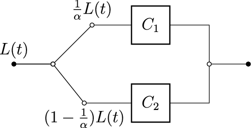
(i) Load-sharing model. The operation of a parallel system sustains a time-dependent load, which is shared by the surviving components. As time goes by, the components fail to work one by one, and the remaining survival components will suffer an increasing shared load. In this situation, the two-component parallel system is called the ‘load-sharing model’ [Reference Belzunce, Lillo, Ruiz and Shaked5, Reference Schechner28]. As assumed in [Reference Yun and Cha34] and [Reference Zhang and Balakrishnan39], the total load is usually unevenly shared by the components. Inspired by their work, as displayed in Figure 1, we consider a general load-sharing model with two components
 $C_1$
and
$C_2$
sharing the total load
$L(\!\cdot\!)$
with respective proportions
$ {1}/{\alpha}$
and
$1-{1}/{\alpha}$
, where
$\alpha > 1$
. We adopt the linear breakdown rule in [Reference Birnbaum and Saunders9], and assume that the total load
$L(\!\cdot\!)$
can be regarded as a fictitious system’s failure rate (see [Reference Schechner28]). Then the lifetime of component
$C_1$
that shares the load
$L(\!\cdot\!)/\alpha$
is denoted by
$T_{L/\alpha}$
with survival function
where
\begin{equation*}\overline F_{T_{L/\alpha}} (t)=\exp \biggl\{-\int_{0}^{t} \dfrac {L(x)}{\alpha} \,\mathrm{d} x\biggr\}, \quad \alpha > 1,\end{equation*}
$L(x)/\alpha$
is interpreted as the instantaneous failure rate of component
$C_1$
at time x under the total load L(x). Furthermore, when one component (say
$C_1$
) fails, the lifetime of the other surviving component (say
$C_2$
) functions continuously and bears the total load
$L(\!\cdot\!)$
with survival function
Therefore the survival function of the load-sharing model can be regarded as the relevation of two components
\begin{equation*}\overline F_{T_L}(t)=\exp \biggl\{-\int_{0}^{t} {L(x)} \,\mathrm{d} x\biggr\}.\end{equation*}
$C_1$
and
$C_2$
with respective failure rates
$L(\!\cdot\!)/\alpha$
and
$L(\!\cdot\!)$
([Reference Belzunce, Martnez-Riquelme and Ruiz7]). In this regard, the survival function of the load-sharing model can be expressed as
\begin{align*}\mathbb{P}( T_{L/\alpha} \# T_L> t )&= \overline F_{T_{L/\alpha}} (t) -\overline F_L(t)\int_0^t\dfrac{1}{\overline F_L(x)} \,\mathrm{d} \overline F_{T_{L/\alpha}} (x)\\[3pt] &= \dfrac{\alpha}{\alpha-1} \overline {F}^{{1}/{\alpha}}_L(t)-\dfrac{1}{\alpha-1}\overline {F}_L(t), \quad\alpha > 1.\end{align*}
-
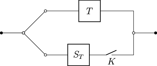
(ii) Minimal repair. Consider a minimal repair policy as shown in Figure 2, where the component with lifetime T starts working first. When the component fails, the switch K will be turned on immediately (the switching time is negligible) so that it is replaced by another component with lifetime S having the same reliability function and same age as T. That is, the component is ‘minimally repaired’ and brought to the working state immediately before failure. Then the resulting reliability under a minimal repair reads as
which is also a special case of relevation.
\begin{equation*}\mathbb{P} (T+S_{T}>t )=\overline {F}(t)+\overline {F}(t)\int_{0}^{t} \dfrac{f(x) }{\overline {F}(x)} \,\mathrm{d} x=\overline {F}(t)-\overline {F}(t) \ln \overline {F}(t),\end{equation*}
Figure 1:Load-sharing model.
Figure 2:Minimal repair.


Recently, Belzunce, Martínez-Riquelme, and Ruiz [Reference Belzunce, Martnez-Riquelme and Ruiz7] considered the problem of where to allocate one relevation in a coherent system in order to enhance system reliability in the sense of the usual stochastic ordering. Sufficient conditions are established on the lifetimes of the original components and the relevation by means of the usual stochastic ordering and the hazard rate ordering. In particular, both the load-sharing model and minimal repair are studied in detail. A natural interesting question arises: If we allocate more than one relevation in a coherent system, what is the best allocation policy? The main objective of this paper is to pinpoint the optimal allocation of a fixed number of relevations in coherent systems by means of the hazard rate order and the usual stochastic order, which partially answers the open problems proposed in [Reference Belzunce, Martnez-Riquelme and Ruiz7]. Moreover, the special cases of the load-sharing model and the minimal repair policy are investigated explicitly.
The remainder of the paper is organized as follows. In the remaining part of this section, we provide some relevant definitions and concepts used below. In Section 2 we study the best allocation policy of two relevations in series systems and establish sufficient (and necessary) conditions for the hazard rate ordering among different allocation policies. Two special cases including the load-sharing and minimal repair policies are also studied when we consider the allocation of one relevation. Section 3 presents the results on optimal allocation of relevations in coherent systems. Section 4 concludes the paper.
Throughout, we assume that all random variables are non-negative and absolutely continuous. We shall use ‘
 $\overset{\operatorname{sgn}}=$
’ to express that both sides of the equality have the same sign, and ‘
 ${\mathrm{d}\phi(t)}/{\mathrm{d}t} $
’ to denote the differentiation of
 $\phi(t)$
with respective to t. The terms ‘increasing’ and ‘decreasing’ mean ‘non-decreasing’ and ‘non-increasing’, respectively. We denote
 $\mathbb{R}=(-\infty,\infty)$
and
 $\mathbb{R}_+=[0,\infty)$
.
Stochastic orders are a very useful tool to compare random variables arising from reliability theory, operations research, actuarial science, economics, finance, and so on. Let X and Y be two random variables with distribution functions F(t) and G(t), survival functions
 $\overline F(t) =1- F(t)$
and
 $\overline G(t) =1- G(t)$
, probability density functions f(t) and g(t), hazard rate functions
 $h_X(t) = f(t) /\overline F(t) $
and
 $h_Y(t) = g(t)/\overline G(t)$
, and reversed hazard rate functions
 $\tilde r_X(t) = f(t) / F(t) $
and
 $\tilde r_Y(t) = g(t)/ G(t)$
, respectively.
Definition 1. X is said to be smaller than Y in the
-
(i) usual stochastic order (denoted by
$X \le_{st} Y$
) if
$\overline {F}(t) \leq \overline {G}(t)$
for all
$t\in\mathbb{R}$
, -
(ii) hazard rate order (denoted by
$X\leq_{hr}Y$
) if
$h_{X}(t)\ge h_{Y}(t)$
for all
$t\in\mathbb{R}$
, or equivalently if
$\overline {G}(t)/\overline {F}(t)$
is increasing in
$t\in\mathbb{R}$
, -
(iii) reversed hazard rate order (denoted by
$X\leq_{rh}Y$
) if
$\tilde r_{X}(t)\le \tilde r_{Y}(t)$
for all
$t\in\mathbb{R}$
, or equivalently if
$ {G}(t)/ {F}(t)$
is increasing in
$t\in\mathbb{R}$
.


It is well known that the (reversed) hazard rate order implies the usual stochastic order, but the reversed statement is not true in general. For more comprehensive discussions of various stochastic orders and their applications, one may refer to the monographs by Shaked and Shanthikumar [Reference Shaked and Shanthikumar29] and Belzunce, Riquelme, and Mulero [Reference Belzunce, Riquelme and Mulero8].
The notion totally positive of order 2 (TP
 $_2$
) plays a prominent role in building various inequalities arising from many research areas. A pair of measurable non-negative real-valued functions
 $(g_1, g_2 )$
are said to satisfy the TP
 $_2$
property if
 $g_1(x_1) g_2(x_2)\ge g_1(x_2) g_2(x_1)$
for all
 $x_1 \le x_2$
.
The following lemma is helpful in building the main results.
Lemma 1. ([Reference Joag-dev, Kochar and Proschan17].) Let
 $(g_1, g_2)$
be a pair of non-negative functions satisfying the TP
 $_2$
property. Let
 $\overline F_\theta$
be the survival function of the random variable
 $X_{\theta}$
, for
 $\theta=1,2$
. Suppose that
 $\overline F_\theta( t)$
is TP
 $_2$
in
 $(\theta, t)$
, and
 $\int_0^\infty g_i(t)\,\mathrm{d} F_\theta(t) $
exists and is finite, for
 $i = 1, 2$
and
 $\theta=1, 2$
. Further, suppose that
 $g_1(t)$
is increasing in t. Then
 $h_i(\theta)=\int_0^\infty g_i(t)\,\mathrm{d} F_\theta(t) $
is TP
 $_2$
in
 $(i,\theta)$
, that is,
 \begin{equation*} \int_0^\infty g_1(t)\,\mathrm{d} F_1(t) \int_0^\infty g_2(t)\,\mathrm{d} F_2(t) \ge\int_0^\infty g_1(t)\,\mathrm{d} F_2(t) \int_0^\infty g_2(t)\,\mathrm{d} F_1(t).\end{equation*}
For detailed discussions of properties of TP
 $_2$
and its applications, we refer interested readers to [Reference Joag-dev, Kochar and Proschan17] and [Reference Karrlin19].
2. Allocation of relevations in series systems
In this section we study optimal allocation of relevations for series systems in terms of the usual stochastic order and the hazard rate order. Henceforth we assume that all components and relevations are independent of each other.
2.1. Allocation of two relevations in series systems
First we provide a result for the usual stochastic ordering among different allocations of two relevations in an n-component series system.
Theorem 1. Let
 $T_1,T_2, \ldots, T_n$
be the lifetimes of n components with survival functions
 $\overline F_1, \overline F_2,$
 $\ldots, \overline F_n$
, respectively, in a series system. Let
 $S_1$
and
 $S_2$
be the lifetimes of two relevations with survival functions
 $ \overline G_1$
and
 $\overline G_2$
, respectively. Denote
 \begin{equation*}V_1=\min \{ T_1\#S_1, T_2\#S_2, T_3, \ldots, T_n \} \end{equation*}
and
 \begin{equation*}V_2=\min \{T_1\#S_2, T_2\#S_1, T_3, \ldots, T_n \}.\end{equation*}
If
 $T_1 \le_{hr} T_2$
and
 $S_1 \ge_{hr} S_2$
, then
 $V_1 \ge_{st} V_2.$
Proof. The survival functions of
 $V_1$
and
 $V_2$
can be expressed as
 \begin{equation*}\overline H_{V_1}(t) =\prod_{ l=3 }^n \overline F_l(t) \biggl\{ \biggl( \overline F_1(t) + \overline G_1(t)\int_0^t \dfrac{f_1( u )}{\overline G_1( u )} \,\mathrm{d} u \biggr)\biggl( \overline F_2(t) + \overline G_2(t)\int_0^t \dfrac{f_2( u )}{\overline G_2( u )} \,\mathrm{d} u \biggr) \biggr\} \end{equation*}
and
 \begin{equation*} \overline H_{V_2}(t) =\prod_{ l=3 }^n \overline F_l(t) \biggl\{ \biggl( \overline F_1(t) + \overline G_2(t)\int_0^t \dfrac{f_1( u )}{\overline G_2( u )} \,\mathrm{d} u \biggr)\biggl( \overline F_2(t) + \overline G_1(t)\int_0^t \dfrac{f_2( u )}{\overline G_1( u )} \,\mathrm{d} u \biggr) \biggr\} ,\end{equation*}
respectively. Observe that
 \begin{align*}&\overline H_{V_1}(t)-\overline H_{V_2}(t) \\[2pt]&\quad \overset{\operatorname{sgn}}= \biggl( \overline F_1(t) + \overline G_1(t)\int_0^t \dfrac{f_1( u )}{\overline G_1( u )} \,\mathrm{d} u \biggr)\biggl( \overline F_2(t) + \overline G_2(t)\int_0^t \dfrac{f_2( u )}{\overline G_2( u )} \,\mathrm{d} u \biggr)\\[2pt]& \quad\quad\, -\biggl( \overline F_1(t) + \overline G_2(t)\int_0^t \dfrac{f_1( u )}{\overline G_2( u )} \,\mathrm{d} u \biggr)\biggl( \overline F_2(t) + \overline G_1(t)\int_0^t \dfrac{f_2( u )}{\overline G_1( u )} \,\mathrm{d} u \biggr)\\&\quad = \overline F_1(t)\overline F_2(t) + \overline F_1(t){{\overline G}_2}(t)\int_0^t {\dfrac{{f_2(u)}}{{\overline G_2(u)}}} \,\mathrm{d} u + \overline F_2(t)\overline G_1(t)\int_0^t {\dfrac{{ f_1(u)}}{{\overline G_1(u)}}} \,\mathrm{d} u \\[2pt]&\quad\quad \, + \overline G_1(t)\overline G_2(t)\int_0^t {\dfrac{{ f_1(u)}}{{\overline G_1(u)}}} \,\mathrm{d} u\int_0^t {\dfrac{{f_2(u)}}{{\overline G_2(u)}}} \,\mathrm{d} u \\[2pt]& \quad\quad\, - \biggl( \overline F_1(t)\overline F_2(t) + \overline F_1(t)\overline G_1(t)\int_0^t {\dfrac{{ f_2(u)}}{{\overline G_1(u)}}} \,\mathrm{d} u + \overline F_2(t)\overline G_2(t)\int_0^t {\dfrac{{ f_1(u)}}{{\overline G_2(u)}}} \,\mathrm{d} u \\[2pt]&\quad\quad\quad\ \ + \overline G_1(t)\overline G_2(t)\int_0^t {\dfrac{{ f_1(u)}}{{\overline G_2(u)}}} \,\mathrm{d} u\int_0^t {\dfrac{{ f_2(u)}}{{\overline G_1(u)}}} \,\mathrm{d} u \biggr) \\&\quad = \int_0^t {\overline F_1(t) f_2(u) \biggl[ {\dfrac{{\overline G_2(t)}}{{\overline G_2(u)}} - \dfrac{{\overline G_1(t)}}{{\overline G_1(u)}}} \biggr]} \,\mathrm{d} u + \int_0^t {\overline F_2(t) f_1(u) \biggl[ {\dfrac{{\overline G_1(t)}}{{\overline G_1(u)}} - \dfrac{{\overline G_2(t)}}{{\overline G_2(u)}}} \biggr]} \,\mathrm{d} u \\[2pt]& \quad\quad\, + \overline G_1(t)\overline G_2(t) \biggl[ {\int_0^t {\dfrac{{ f_1(u)}}{{\overline G_1(u)}}} \,\mathrm{d} u\int_0^t {\dfrac{{ f_2(u)}}{{\overline G_2(u)}}} \,\mathrm{d} u - \int_0^t {\dfrac{{ f_1(u)}}{{\overline G_2(u)}}} \,\mathrm{d} u\int_0^t {\dfrac{{ f_2(u)}}{{\overline G_1(u)}}} \,\mathrm{d} u} \biggr] \\&\quad = \int_0^t { \bigl[ {\overline F_2(t) f_1(u) - \overline F_1(t) f_2(u)} \bigr] \biggl[ {\dfrac{{\overline G_1(t)}}{{\overline G_1(u)}} - \dfrac{{\overline G_2(t)}}{{\overline G_2(u)}}} \biggr]} \,\mathrm{d} u \\[2pt]&\quad\quad\, + \overline G_1(t)\overline G_2(t) \biggl[ {\int_0^t {\dfrac{{ f_1(u)}}{{\overline G_1(u)}}} \,\mathrm{d} u\int_0^t {\dfrac{{ f_2(u)}}{{\overline G_2(u)}}} \,\mathrm{d} u - \int_0^t {\dfrac{{ f_1(u)}}{{\overline G_2(u)}}} \,\mathrm{d} u\int_0^t {\dfrac{{ f_2(u)}}{{\overline G_1(u)}}} \,\mathrm{d} u} \biggr]\\[2pt]&\quad {=\!:}\, \phi_1(t)+\phi_2(t),\end{align*}
where
 \begin{equation*}\phi_1(t) = \int_0^t { \bigl[{\overline F_2(t)f_1(u) - \overline F_1(t)f_2(u)} \bigr] \biggl[ {\dfrac{\overline G_1(t)}{\overline G_1(u)} - \dfrac{\overline G_2(t)}{\overline G_2(u)}} \biggr]} \,\mathrm{d} u\end{equation*}
and
 \begin{equation*}\phi_2(t)=\overline G_1(t)\overline G_2(t) \biggl[ {\int_0^t {\dfrac{f_1(u)}{\overline G_1(u)}} \,\mathrm{d} u\int_0^t {\dfrac{f_2(u)}{\overline G_2(u)}} \,\mathrm{d} u - \int_0^t {\dfrac{f_1(u)}{\overline G_2(u)}} \,\mathrm{d} u\int_0^t {\dfrac{f_2(u)}{\overline G_1(u)}} \,\mathrm{d} u} \biggr] .\end{equation*}
Note that
 $T_1 \le _{hr} T_2$
implies
 $ {\overline F_2(t)f_1(u) - \overline F_1(t)f_2(u)} \ge 0$
for all
 $ 0 \le u \le t$
. On the other hand,
 $S_1 \ge_{hr} S_2$
is equivalent to
 \begin{equation*}\dfrac{\overline G_1(t)}{\overline G_2(t)} \ge \dfrac{\overline G_1(u)}{\overline G_2(u)}\quad\text{for all } 0 \le u \le t, \end{equation*}
that is,
 \begin{equation*} {\dfrac{\overline G_1(t)}{\overline G_1(u)} - \dfrac{\overline G_2(t)}{\overline G_2(u)}} \end{equation*}
is also non-negative, for all
 $ 0 \le u \le t$
. Hence
 $\phi_1(t)$
is non-negative for all
 $t\in\mathbb{R}_+$
.
Observe that
 \begin{align*}\phi_2(t) & \overset{\operatorname{sgn}}= {\int_0^t {\dfrac{f_1(u)}{\overline G_1(u)}} \,\mathrm{d} u\int_0^t {\dfrac{f_2(u)}{\overline G_2(u)}} \,\mathrm{d} u - \int_0^t {\dfrac{f_1(u)}{\overline G_2(u)}} \,\mathrm{d} u\int_0^t {\dfrac{f_2(u)}{\overline G_1(u)}} \,\mathrm{d} u}.\end{align*}
According to
 $S_1 \ge_{hr} S_2$
, we have
 \begin{equation*} \dfrac{1}{{\overline G_1 (x)\overline G_2 (y)}} - \dfrac{1}{{\overline G_1 (y)\overline G_2 (x)}} = \dfrac{{\overline G_1 (y)\overline G_2 (x) - \overline G_1 (x)\overline G_2 (y)}}{{\overline G_1 (x)\overline G_2 (y)\overline G_1 (y)\overline G_2 (x)}} \ge 0 \quad \text{for } x \le y ,\end{equation*}
from which it follows that
 $ ( 1/{\overline G_1},1/{\overline G_2} ) $
is a pair of non-negative functions satisfying the TP
 $_2$
property. Further,
 $T_1 \le_{hr} T_2$
implies that the survival function of
 $\overline F_\theta(t)$
is TP
 $_2$
in
 $(\theta, t)$
. Since
 ${1}/{\overline G_1(t)}$
is increasing for
 $t\in\mathbb{R}_+$
, according to Lemma 1 we know that
 $\phi_2(t)$
is non-negative for all
 $t\in\mathbb{R}_+$
. To sum up, for all
 $t\in\mathbb{R}_+$
,
 \begin{equation*} \overline H_{V_1}(t) - \overline H_{V_2}(t) =\phi_1(t)+\phi_2(t) \ge 0, \end{equation*}
and thus the proof is completed.
The following numerical example illustrates Theorem 1.
Example 1. Consider allocating two relevations in a series system with two independent components. Assume that
 $T_1$
and
 $T_2$
have respective survival functions
 \begin{equation*} \overline F_1(t)={\operatorname{exp}}\biggl\{{-\int_0^t (3 x^2+3 x+5 ) \,\mathrm{d}x}\biggr\} ,\quad \overline F_2(t)={\operatorname{exp}}\biggl\{{-\int_0^t (3 x^2+2 x+2 ) \,\mathrm{d} x}\biggr\}, \end{equation*}
and
 $S_1$
and
 $S_2$
have responding survival functions
 \begin{equation*} \overline G_1(t)={\operatorname{exp}}\biggl\{{-\int_0^t (5 x^2+2 x+1 ) \,\mathrm{d} x}\biggr\} , \quad \overline G_2(t)= {\operatorname{exp}}\biggl\{{-\int_0^t (5 x^2+4 x+3 ) \,\mathrm{d} x}\biggr\}. \end{equation*}
It is obvious that both
 $\overline F_2(t) / \overline F_1(t) ={\mathrm{e}}^{{t^2}/{2}+3 t} $
and
 $ \overline G_1(t) / \overline G_2(t)={\mathrm{e}}^{t^2+2 t} $
are increasing in
 $t \in\mathbb{R}_+$
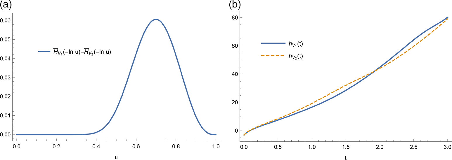
. From Figure 3(a) we can see that the difference of survival functions
 $\overline H_{V_1}(t) - \overline H_{V_2}(t)$
is always non-negative for all
 $t=-\ln u$
and
 $u\in[0,1]$
. Thus the relevation with lifetime
 $S_1$
should be moved to the location of the component with lifetime
 $T_1$
, which is in accordance with the usual stochastic ordering result of Theorem 1. However, the hazard rate functions
 $h_{V_1}(t)$
and
 $h_{V_2}(t)$
intersect, as shown in Figure 3(b), which indicates that the hazard rate ordering does not hold between
 $ {V_1}$
and
 ${V_2}$
.
(a) Plot of the difference function
 $\overline H_{V_1}(-\ln u) - \overline H_{V_2}(-\ln u)$
for
 $u\in[0,1]$
. (b) Plot of the hazard rate functions
 $h_{V_1}(t)$
and
 $ h_{V_2}(t)$
for
 $t\in[0,3]$
.

Remark 1. For a series system with components having ordered lifetimes
 $ T_1 \le_{hr} T_2 \le_{hr} \cdots \le_{hr} T_n$
, and two relevations with lifetimes such that
 $S_1 \ge_{hr} S_2$
, Theorem 1 states that the relevation with smaller failure rate should be put on the worst component (having largest failure rate) in order to improve system reliability in the sense of the usual stochastic ordering. This finding agrees with the classical allocation results of hot standbys, cold standbys, and minimal repairs; see for example [Reference Boland, El-Neweihi and Proschan10], [Reference Zhang, Zhang and Fang35], and [Reference Zhang and Zhao38]. It might be of great interest to relax the assumptions in Theorem 1 when one considers the load-sharing model or the minimal repair policy. We leave them as open problems.
Let
 $\boldsymbol \pi=(\pi_1, \pi_2,\ldots, \pi_n)$
be a permutation of
 $\{1, 2, \ldots, n\}$
,
 $\boldsymbol \pi^+=\{1, 2, \ldots, n\}$
, and
 $\boldsymbol \pi^-=\{n, n-1, \ldots, 1\}$
. Consider a series system with n components having respective lifetimes
 $T_1, T_2, \ldots,T_n$
, which are allocated n relevations with lifetimes
 $S_1,S_2, \ldots, S_n$
. Assume that each component is only allocated by one relevation, hence there exist
 $n!$
different relevation policies. Let
 ${\textbf{T}}\#\textbf{S}_{\boldsymbol \pi}=(T_1\#S_{\pi_1}, T_1\#S_{\pi_2}, \ldots, T_1\#S_{\pi_n})$
be the lifetime of the resulting components under the allocation policy that the relevation with lifetime
 $S_{\pi_i}$
is allocated to the component with lifetime
 $T_i$
,
 $i=1,2,\ldots,n$
. The following corollary immediately follows from Theorem 1.
Corollary 1. If
 $T_1 \le_{hr} T_2 \le_{hr} \cdots \le_{hr}T_n$
and
 $S_1 \ge_{hr} S_2 \ge_{hr} \cdots \ge_{hr}S_n$
, then
 \begin{equation*}\textbf{T}\#\textbf{S}_{\boldsymbol \pi^-} \le_{st} \textbf{T}\#\textbf{S}_{\boldsymbol \pi} \le_{st} \textbf{T}\#\textbf{S}_{\boldsymbol \pi^+},\end{equation*}
that is,
 $\textbf{T}\#\textbf{S}_{\boldsymbol \pi^+}$
is the best allocation policy, and
 $\textbf{T}\#\textbf{S}_{\boldsymbol \pi^-}$
is the worst allocation policy within the class of all admissible allocations, where
 \begin{equation*}\textbf{T}\#\textbf{S}_{\boldsymbol \pi^+}=\min \{ T_1\#S_1, T_2\#S_2, \ldots, T_{n-1}\#S_{n-1}, T_n\#S_n \}\end{equation*}
and
 \begin{equation*}\textbf{T}\#\textbf{S}_{\boldsymbol \pi^-}=\min \{ T_1\#S_n, T_2\#S_{n-1}, \ldots, T_{n-1}\#S_{2},T_n\#S_1 \}. \end{equation*}
Proof. Note that the lexicographic permutation order starts from the identity permutation
 $\boldsymbol \pi^+=(1,2,\ldots, n)$
. By successively swapping only two numbers we obtain all possible permutations, that is, the vector
 $\boldsymbol \pi$
can be obtained by successively exchanging two coordinates of
 $\boldsymbol \pi^+$
for finite times. The last permutation in lexicographic order will be the permutation with all numbers in reversed order, i.e.
 $\boldsymbol \pi^-=(n,n-1,\ldots,2,1)$
. Then the result can be obtained immediately from Theorem 1.
2.2. Allocation of one relevation in series systems: load-sharing model
Next we investigate the sufficient and necessary conditions for the usual stochastic ordering and the hazard rate ordering under the load-sharing model.
For the sake of convenience, let us define
 \begin{equation*}\gamma_{T_i}(t)=\frac {\alpha -\overline F_i^{1- {1}/{\alpha}}(t)}{h_i(t)} \quad \text{for}\ \ i=1,2,\end{equation*}
where
 $\overline F_i(t)$
and
 ${h_i}(t) $
are the survival function and the hazard rate function, respectively, of random variable
 ${T_i}$
.
Theorem 2. Let
 $T_1,T_2, \ldots, T_n$
be the lifetimes of n components with survival functions
 $ \overline F_1, \overline F_2,$
 $\ldots, \overline F_n$
, respectively, in a series system. The load-sharing model of the component with lifetime
 $T_i$
is denoted by
 $T_{i, L/\alpha}\#T_i $
, for
 $i=1,2$
and
 $\alpha>1$
. Denote
 $U_1=\min \{T_{1, L/\alpha}\#T_1, T_2, \ldots, T_n\}$
and
 $U_2=\min \{T_1,T_{2, L/\alpha}\#T_2, \ldots, T_n\}.$
Then
-
(i)
$U_1 \ge_{st} U_2$
if and only if
$T_1 \le_{st}T_2$
, -
(ii)
$U_1 \ge_{hr} U_2$
if and only if
$\gamma_{T_1}(t) \le \gamma_{T_2}(t)$
for all
$t\in\mathbb{R}_+$
.


Proof. (i) Let
 $\overline H_{U_1}(t)$
and
 $\overline H_{U_2}(t)$
denote the survival functions of the load-sharing policies
 $U_1$
and
 $U_2$
, respectively. Then
 \begin{equation*}\overline {H}_{U_1}(t)=\prod_{ l=3 }^n \overline F_l(t) \biggl\{ \biggl(\dfrac{\alpha}{\alpha-1} \overline F_1^{{1}/{\alpha}}(t)-\dfrac{1}{\alpha-1} \overline F_1(t)\biggr) \overline F_2(t) \biggr\} \end{equation*}
and
 \begin{equation*}\overline {H}_{U_2}(t)=\prod_{ l=3 }^n \overline F_l(t) \biggl\{ \biggl(\dfrac{\alpha}{\alpha-1} { \overline F_2}^{{1}/{\alpha}}(t)-\dfrac{1}{\alpha-1} { \overline F_2}(t)\biggr) { \overline F_1}(t) \biggr\}.\end{equation*}
It is obvious that, for
 $\alpha>1$
,
 \begin{align*}\phi_3(t)&\,{:\!=}\, {\overline {H}_{U_1}(t)}-{\overline {H}_{U_2}(t)} \\[3pt]&\overset{\operatorname{sgn}}= \overline F_2(t)\biggl(\dfrac{\alpha}{\alpha-1} \overline F_1^{{1}/{\alpha}}(t)-\dfrac{1}{\alpha-1} \overline F_1(t)\biggr)-\overline F_1(t)\biggl(\dfrac{\alpha}{\alpha-1} \overline F_2^{{1}/{\alpha}}(t)-\dfrac{1}{\alpha-1} \overline F_2(t)\biggr)\\[3pt]& = \dfrac{\alpha}{\alpha-1} \overline F_1(t) \overline F_2(t)(\overline F_1^{{1}/{\alpha}-1}(t)-\overline F_2^{{1}/{\alpha}-1}(t))\end{align*}
is non-negative if and only if
 ${ \overline F_1}(t) \le { \overline F_2}(t)$
for all
 $t\in\mathbb{R}_+$
. Hence the proof is completed.
(ii) The desired result is equivalent to proving the increasing monotonicity of the function
 \begin{align*}\phi_4(t)&\,{:\!=}\, \dfrac{\overline {H}_{U_1}(t)}{\overline {H}_{U_2}(t)} =\dfrac{\bigl(\frac{\alpha}{\alpha-1} { \overline F_1}^{{1}/{\alpha}}(t)-\frac{1}{\alpha-1}{ \overline F_1}(t)\bigr) { \overline F_2}(t)}{\bigl(\frac{\alpha}{\alpha-1} { \overline F_2}^{{1}/{\alpha}}(t)-\frac{1}{\alpha-1}{ \overline F_2}(t)\bigr) { \overline F_1}(t)}\\[3pt]&= \dfrac{\bigl(\frac{\alpha}{\alpha-1} { \overline F_1}^{{1}/{\alpha}-1}(t)-\frac{1}{\alpha-1} \bigr){\overline F_1}(t) \overline F_2(t) } {\bigl(\frac{\alpha}{\alpha-1} { \overline F_2}^{{1}/{\alpha}-1}(t)-\frac{1}{\alpha-1} \bigr){\overline F_2}(t) \overline F_1(t)}=\dfrac{\alpha { \overline F_1}^{{1}/{\alpha}-1}(t)-1 } {\alpha { \overline F_2}^{{1}/{\alpha}-1}(t)-1 }.\end{align*}
Note that
 \begin{align*}\dfrac{\mathrm{d}\phi_4(t)}{\mathrm{d}t}&\overset{\operatorname{sgn}}= (\alpha-1)h_{1}(t){ \overline F_1}^{{1}/{\alpha}-1}(t)(\alpha { \overline F_2}^{{1}/{\alpha}-1}(t)-1)\\[3pt]& \quad\, -(\alpha-1)h_{2}(t){ \overline F_2}^{{1}/{\alpha}-1}(t)(\alpha { \overline F_1}^{{1}/{\alpha}-1}(t)-1)\\[3pt]&\overset{\operatorname{sgn}}= h_{1}(t){ \overline F_1}^{{1}/{\alpha}-1}(t)(\alpha { \overline F_2}^{{1}/{\alpha}-1}(t)-1)-h_{2}(t){ \overline F_2}^{{1}/{\alpha}-1}(t)(\alpha { \overline F_1}^{{1}/{\alpha}-1}(t)-1),\end{align*}
where
 $h_{i}(t)=f_i(t)/\overline F_i(t)$
is the hazard rate function of
 $T_i$
, for
 $i=1,2$
. The non-negativity of
 $ {\mathrm{d}\phi_4(t)}/{\mathrm{d}t} $
is equivalent to
 \begin{equation*} h_{1}(t){ \overline F_1}^{{1}/{\alpha}-1}(t)\bigl(\alpha { \overline F_2}^{{1}/{\alpha}-1}(t)-1\bigr)\ge h_{2}(t){ \overline F_2}^{{1}/{\alpha}-1}(t)\bigl(\alpha { \overline F_1}^{{1}/{\alpha}-1}(t)-1\bigr), \end{equation*}
that is,
 \begin{equation*}\dfrac{\alpha -{ \overline F_2}^{1-{1}/{\alpha}}(t)}{ h_{2}(t)} \ge \dfrac{\alpha -{ \overline F_1}^{1-{1}/{\alpha}}(t)}{ h_{1}(t)}. \end{equation*}
It is clear that
 $ {\mathrm{d}\phi_4(t)}/{\mathrm{d}t} \ge 0 $
is equivalent to
 $U_1 \ge_{hr} U_2$
, which holds if and only if
 $\gamma_{T_1}(t) \le \gamma_{T_2}(t)$
, for all
 $t\in\mathbb{R}_+$
.
Remark 2. Theorem 2(i) extends the result of Lemma 3 of [Reference Belzunce, Martnez-Riquelme and Ruiz7] to the case of the general load-sharing model. Further, Theorem 2(ii) established sufficient and necessary conditions for the hazard rate ordering.
It is natural to ask whether the assumption in Theorem 2(ii) implies or can be implied by the hazard rate order. The following numerical example provides a negative answer.
Example 2. Assume that
 $T_1$
and
 $T_2$
have survival functions
 $\overline F_1(t) = {\mathrm{e}}^{-({t}/{\beta_1})^{\lambda_1}}$
and
 $\overline F_2(t) = {\mathrm{e}}^{- ({t}/{\beta_2} )^{\lambda_2}}$
, respectively, for
 $t\in \mathbb R_+$
.
-
(i) Setting
$\lambda_1=8$
,
$\beta_1=2$
,
$\lambda_2=3$
, and
$\beta_2=1$
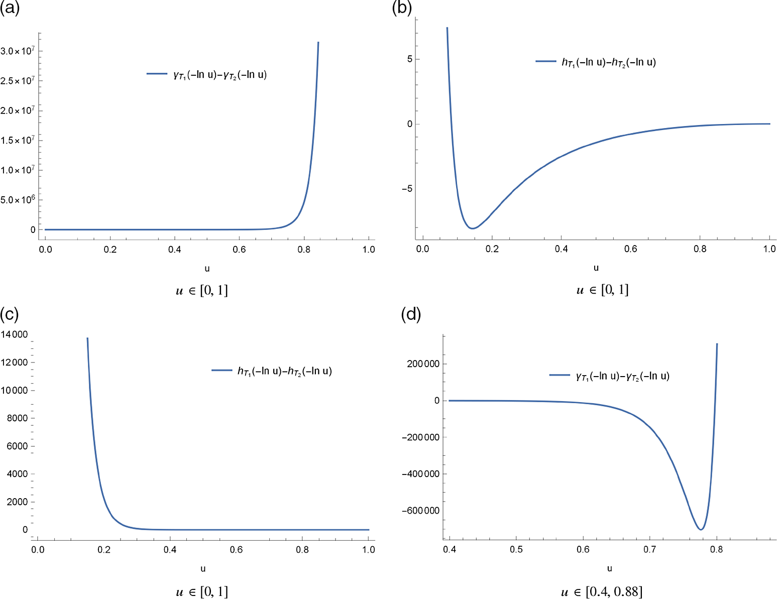
, from Figures 4(a) and 4(b) we see that the difference function
$ \gamma_{T_1}(t) - \gamma_{T_2}(t) $
is always non-negative; however, the difference function
$ h_{T_1}(t) - h_{T_2}(t) $
crosses at the line
$y=0$
, for
$t=-\ln u$
and
$u\in[0,1]$
. Hence
$ \gamma_{T_1}(t) \ge \gamma_{T_2}(t) $
implies neither
$T_1 \ge_{hr} T_2$
nor
$T_1 \le_{hr} T_2$
. -
(ii) Taking
$\lambda_1=12$
,
$\beta_1=1$
,
$\lambda_2=8$
, and
$\beta_2=2$
, Figures 4(c) and 4(d) show that the difference function
$ h_{T_1}(t) - h_{T_2}(t) $
is always non-negative for all
$t=-\ln u$
and
$u\in[0,1]$
, while the difference function
$ \gamma_{T_1}(t) - \gamma_{T_2}(t) $
crosses at the line
$y=0$
, for
$t=-\ln u$
and
$u\in[0.4,0.88]$
. Thus
$ {T_1} \le_{hr} {T_2}$
implies neither
$\gamma_{T_1}(t) \ge \gamma_{T_2}(t)$
nor
$\gamma_{T_1}(t) \le \gamma_{T_2}(t)$
.


Plots of the difference functions
 $\gamma_{T_1}(-\ln u)- \gamma_{T_2}(-\ln u)$
and
 $h_{T_1}(-\ln u)-h_{T_2}(-\ln u) $
for
 $u\in[0,1]$
.

Therefore it follows from (i) and (ii) that the condition
 $ \gamma_{T_1}(t) \le \gamma_{T_2}(t)$
for all
 $t\in\mathbb{R}_+$
does not imply or is not implied by
 $T_1 \le_{hr} T_2$
.
The next example not only illustrates the result of Theorem 2 but also indicates that the reversed hazard rate ordering does not hold in general under the same assumption.
Example 3. Consider the load-sharing model in a series system with two independent components. Assume that the survival functions of
 $T_1$
and
 $T_2$
are
 \begin{equation*} \overline F_1(t)={\operatorname{exp}}\biggl\{-\int_0^t (5x^2+17x+1 ) \,\mathrm{d}x\biggr\} \quad\text{and}\quad \overline F_2(t)={\operatorname{exp}}\biggl\{-\int_0^t (2 x^2+5 x ) \,\mathrm{d} x\biggr\} , \end{equation*}
respectively, for
 $t\in\mathbb{R}_+$
.
-
(i) The difference functions
$ \gamma_{T_1}(t) - \gamma_{T_2}(t) $
and
$h_{U_1}(t) -h_{U_2}(t)$
are plotted in Figures 5(a) and 5(b) for
$t=-\ln u$
and
$u\in[0,1]$
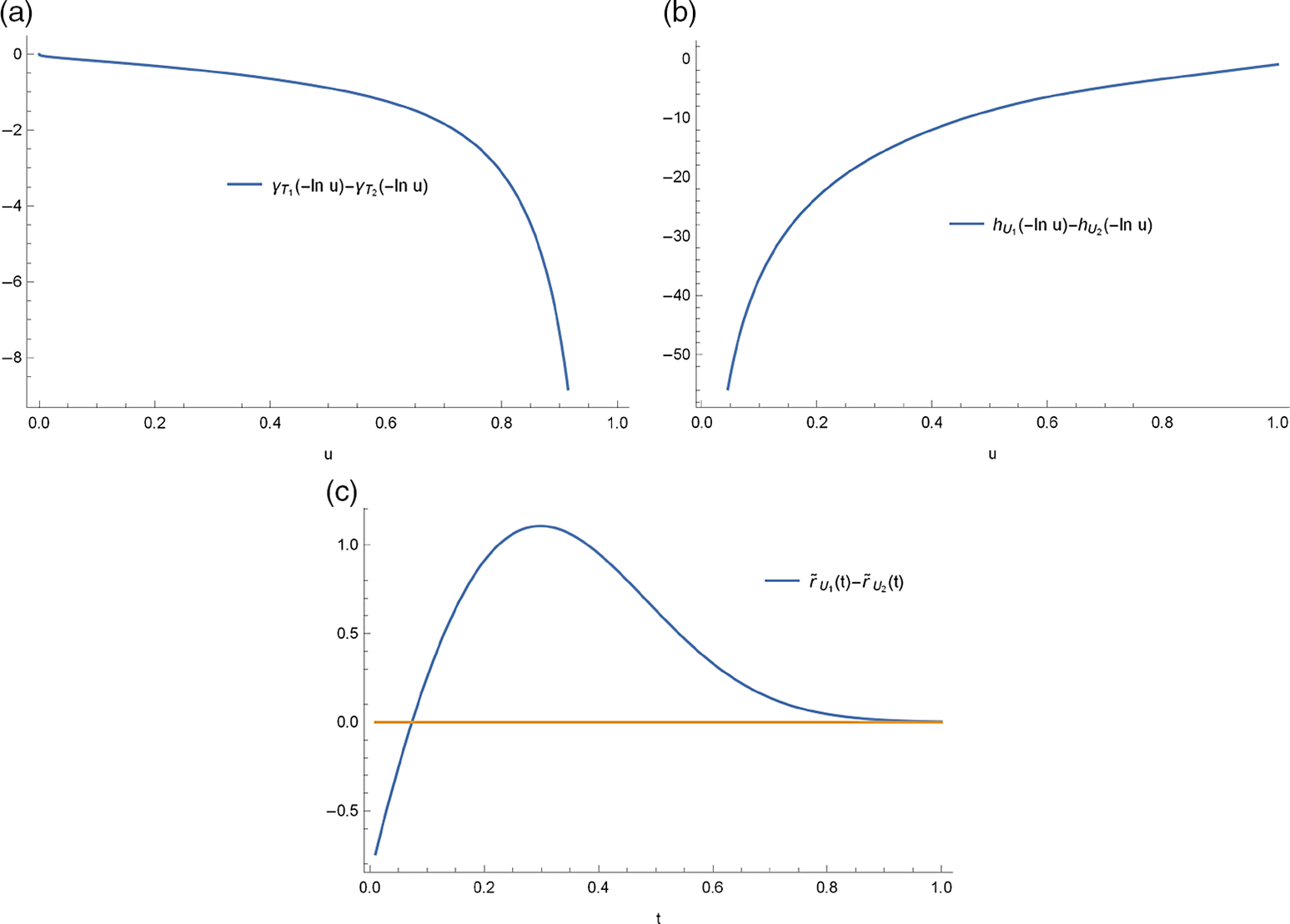
, from which we can see that both difference functions are always non-positive, which is in accordance with the result of Theorem 2. -
(ii) A natural question arises: Does the reversed hazard rate ordering hold in the setting of Theorem 2? Let
$ \tilde r_{U_i}(t)$
be the reversed hazard rate function of
$U_i$
, for
$i=1,2 $
. However, in the same set-up as (i), the difference function
$\tilde r_{U_1}(t)-\tilde r_{U_2}(t)$
intersects at the line
$y=0$
, as displayed in Figure 5(c), which implies that
$ {U_1} \nleq_{rh} {U_2}$
and
$ {U_1} \ngeq_{rh} {U_2}$
.


(a) Plot of the difference function
 $ \gamma_{T_1}(-\ln u) - \gamma_{T_2}(-\ln u) $
for all
 $u\in[0,1]$
. (b) Plot of the difference function
 $h_{U_1}(-\ln u)- h_{U_2}(-\ln u)$
for all
 $u\in[0,1]$
. (c) Plot of the difference function
 $\tilde r_{U_1}(t)- \tilde r_{U_2}(t)$
for
 $t\in[0,1]$
.

2.3. Allocation of one relevation in series systems: minimal repair
This subsection studies the allocation of one minimal repair in an n-component series system by stochastically optimizing the resulting lifetime by means of the hazard rate order. For the sake of convenience, let us define
 \begin{equation*}\beta_{T_i} (t)=\dfrac{h_i(t)}{1-\ln \overline {F_i}(t)} \quad \text{for $i=1,2$},\end{equation*}
where
 $\overline F_i$
and
 ${h_{i}}$
, respectively, are the survival function and the hazard rate function of
 ${T_i}$
for
 $i=1,2$
.
Theorem 3. Let
 $T_1,T_2, \ldots, T_n$
be the lifetimes of n components with survival functions
 $\overline F_1, \overline F_2,$
 $\ldots, \overline F_n$
, respectively, in a series system. Let
 $S_1, S_2$
be the lifetimes of two minimal repairs with survival functions
 $ \overline F_1$
and
 $\overline F_2$
. Denote
 $M_1=\min\{T_1\#S_1, T_2, T_3, \ldots, T_n\} $
and
 $M_2=\min\{T_1, T_2\#S_2, T_3, \ldots, T_n\}$
. Then
 $M_1 \ge _{hr} M_2$
if and only if
 $\beta_{T_1}(t) \ge \beta_{T_2}(t)$
for all
 $t\in\mathbb{R}_+$
.
Proof. The survival functions of
 $M_1$
and
 $M_2$
can be expressed as
 \begin{equation*}\overline {H}_{M_1}(t)=\prod_{ l=3}^n \overline F_l(t) \biggl\{ \overline {F}_{2}(t) \overline {F}_{1}(t)\biggl(1+\int_{0}^{t} \dfrac{f_{1}(u)}{\overline {F}_{1}(u)} \,\mathrm{d} u\biggr) \biggr\} \end{equation*}
and
 \begin{equation*}\overline {H}_{M_2}(t)=\prod_{ l=3}^n \overline F_l(t) \biggl\{ \overline {F}_{2}(t) \overline {F}_{1}(t)\biggl(1+\int_{0}^{t} \dfrac{f_{2}(u)}{\overline {F}_{2}(u)} \,\mathrm{d} u\biggr) \biggr\},\end{equation*}
respectively. The desired result boils down to proving the increasing monotonicity of
 \begin{equation*}\phi_5(t)\,{:\!=}\,\dfrac{\overline{H}_{M_1}(t)}{\overline {H}_{M_2}(t)}= \dfrac{1-\ln\overline F_1(t)}{1-\ln\overline F_2(t)}. \end{equation*}
Observe that
 \begin{align*}\dfrac{\mathrm{d}\phi_5(t)}{\mathrm{d}t}&\overset{\operatorname{sgn}}= \dfrac{f_1(t)}{\overline F_1(t)}(1-\ln\overline F_2(t))-\dfrac{f_2(t)}{\overline F_2(t)}(1-\ln\overline F_1(t))\\[3pt]&= h_1(t)(1-\ln\overline F_2(t))- h_2(t)(1-\ln\overline F_1(t)).\end{align*}
Thus the non-negativity of
 ${\mathrm{d}\phi_5(t)}/{\mathrm{d}t}$
is equivalent to
 $\beta_{T_1}(t) \ge \beta_{T_2}(t)$
for all
 $t\in\mathbb{R}_+$
, which implies the desired result.
Remark 3. Theorem 3 provides a sufficient and necessary condition for the optimal allocation of a minimal repair in a series system with respect to the hazard rate order, which serves as a nice complement to the usual stochastic ordering result of Lemma 2 in [Reference Belzunce, Martnez-Riquelme and Ruiz7].
One may wonder whether the reversed hazard rate ordering holds in the set-up of Theorem 3. Unfortunately, the following numerical example gives us a negative answer.
Example 4. Suppose a series system is made up of two components with lifetimes
 $ T_1 $
and
 $ T_2 $
having reliability functions
 \begin{equation*} \overline F_1(t)={\operatorname{exp}}\biggl\{-\int_0^t (2 x^3+5 x ) \,\mathrm{d} x\biggr\} \quad\text{and}\quad \overline F_2(t)={\operatorname{exp}}\biggl\{- \biggl(\frac{t}{8} \biggr)^6\biggr\}, \end{equation*}
respectively. Denote
 $\varphi(t)=H_{M_1}(t) / H_{M_2}(t)$
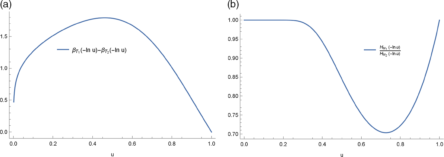
. Although the difference function
 $\beta_{T_1}(t) - \beta_{T_2}(t)$
is always non-negative in Figure 6(a), for
 $t=-\ln u$
and
 $u\in[0,1]$
, the ratio function
 $\varphi(t)$
is not strictly monotone in
 $t=-\ln u$
for
 $u\in[0,1]$
, as shown in Figure 6(b), which indicates that
 $\beta_{T_1}(t) \geq \beta_{T_2}(t)$
for
 $t\in\mathbb{R}_+$
implies neither
 $M_1 \geq _{rh} M_2$
nor
 $M_1 \leq _{rh} M_2$
.
For a parallel system consisting of n independent components, we can develop ordering results similar to those of Theorems 2 and 3 for the load-sharing and minimal repair policies. Define
 \begin{equation*} \delta_{T_i} (t)=\dfrac{\tilde r_i(t)}{1+\ln \overline {F_i}(t)}, \quad i=1,2,\end{equation*}
where
 $\overline F_i$
and
 ${\tilde r_{i}}$
, respectively, are the survival function and the reversed hazard rate function of random variable
 ${T_i}$
.
(a) Plot of the difference function
 $\beta_{T_1}(-\ln u)- \beta_{T_2}(-\ln u)$
for all
 $u \in[0,1]$
. (b) Plot of the ratio function
 $H_{M_1}(-\ln u)/ H_{M_2}(-\ln u)$
for all
 $u \in[0,1]$
.

Proposition 1. Consider a parallel system consisting of n independent components with lifetimes
 $T_1,T_2, \ldots, T_n$
. Let
 $T_{i, L/\alpha}\#T_i$
, for
 $i=1,2$
, denote the lifetime in a load-sharing model for the component with lifetime
 $T_i$
. Let
 \begin{equation*}\tilde{U}_{1}=\max\{T_{1,L/\alpha }\#T_1 , T_2, T_{3}, \ldots, T_n\}\quad{and}\quad \tilde{U}_{2}=\max\{T_1,T_{2,L/\alpha}\#T_2 , T_{3}, \ldots, T_n\}.\end{equation*}
Then
 $\tilde{U}_{1} \le_{st} \tilde{U}_{2}$
if and only if
 $T_1 \le_{st}T_2$
.
Proposition 2. Let
 $T_1,T_2, \ldots, T_n$
be the lifetimes of n components with survival functions
 $\overline F_1, \overline F_2, \ldots, \overline F_n$
, respectively, in a parallel system. Let
 $S_1,S_2$
be the lifetimes corresponding to two minimal repairs with survival functions
 $ \overline F_1$
and
 $\overline F_2$
. Let
 \begin{equation*}\tilde{M}_{1}=\max\{T_1\#S_1, T_2, T_3 \ldots, T_n\}\quad{and}\quad \tilde{M}_{2}=\max\{T_1, T_2\#S_2, T_3 \ldots, T_n\}.\end{equation*}
Then
 $\tilde{M}_{1} \le _{rh}\tilde{M}_{2}$
if and only if
 $ \delta_{T_1}(t) \ge \delta_{T_2}(t)$
for all
 $t\in\mathbb{R}_+$
.
3. Allocation of relevations in coherent systems
In this section we extend the results developed in the previous sections to the case of coherent systems. Let us consider a coherent system made up of n components with lifetimes
 $T_1, T_2, \ldots, T_n$
, structure function
 $\Phi$
, and all minimal path sets
 $P_1, P_2, \ldots, P_k$
, where
 $1\le k \le n$
. According to [Reference Barlow and Proschan2], the lifetime of this coherent system can be expressed as
 \begin{equation*}\tau=\max _{1 \leq j \leq k}\Big\{\min _{i \in P_{j}} T_{i}\Big\}.\end{equation*}
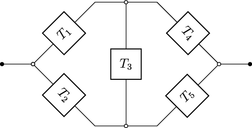
For example, the bridge system (see Figure 7) has minimal path sets
 $P_1 = \{1, 4\}$
,
 $P_2 = \{1,3,5\}$
,
 $P_3 = \{2,5\}$
, and
 $P_4 = \{2,3,4\}$
, which is commonly used in reliability engineering. Then the lifetime of this system can be written as
 \begin{equation*}\tau= \max\{\min\{T_1, T_4 \}, \min\{T_1, T_3,T_5\}, \min\{T_2, T_5\}, \min\{T_2, T_3, T_4 \}\}.\end{equation*}
Bridge system.

For two components located in a common minimal path of a coherent system, the following result establishes the optimal allocation of two relevations in a coherent system in terms of the minimal path sets.
Theorem 4. For a coherent system with structure function
 $ \Phi$
, let
 $P_1, P_2, \ldots, P_k$
be its minimal path sets. Consider two locations
 $i, j\in \{1, 2, \ldots, n \}$
such that
 $i <j$
, and either
 $\{i, j\} \subseteq P_l $
or
 $\{i, j\}\cap P_l =\emptyset$
, for any
 $l = 1, \ldots, k$
. For some minimal path set
 $P_r$
such that
 $\{i, j\} \subseteq P_r $
, we denote the resulting system lifetimes by
 $\tau_1$
and
 $\tau_2$
under two different allocation policies
 \begin{equation*} T_1,\ldots, T_{i-1}, T_i\#S_1, T_{i+1}, \ldots, T_{j-1},T_j\#S_2 , T_{j+1}\ldots, T_n\end{equation*}
and
 \begin{equation*} T_1, \ldots, T_{i-1}, T_i\#S_2, T_{i+1}, \ldots, T_{j-1}, T_j\#S_1, T_{j+1}, \ldots, T_n,\end{equation*}
respectively. If
 $T_i \le_{hr} T_j$
and
 $S_1 \ge_{hr} S_2$
, then
 $\tau_1 \ge_{st} \tau_2$
.
Proof. The idea of the proof is borrowed from Theorem 1 of [Reference Belzunce, Martnez-Riquelme and Ruiz7]. Let
 $V_1=\min\{T_i\#S_1, T_j\#S_2\}$
and
 $V_2=\min\{T_i\#S_2, T_j\#S_1\}$
. Then, for some minimal path set
 $P_l$
such that
 $\{i, j\} \subseteq P_l$
, we have
 \begin{equation*}\tau_1= \min \biggl\{ \underset { m\in P_l, m \ne i,j }{\min} \{T_m\},{T_i\#S_1, T_j\#S_2 } \biggr\}=\min \biggl\{ \underset { m\in P_l, m \ne i,j }{\min} \{T_m\},V_1 \biggr\} \end{equation*}
and
 \begin{equation*} \tau_2=\min \biggl\{ \underset { m\in P_l, m \ne i,j }{\min} \{T_m\},{T_i\#S_2, T_j\#S_1} \biggr\}=\min \biggl\{ \underset { m\in P_l, m \ne i,j }{\min} \{T_m\},V_2 \biggr\} .\end{equation*}
By applying Theorem 1, we obtain that
 $ V_1 \ge_{st} V_2$
, which further implies that
 $\tau_1 \ge_{st} \tau_2$
.
Next we present a numerical example to illustrate Theorem 4.
Example 5. Consider a bridge system with components having lifetimes
 $T_i$
, and let
 $\overline F_i$
be their survival functions, for
 $i=1, \ldots, 5$
. Assume that
 \begin{gather*}\begin{aligned} \overline F_1(t)&={\operatorname{exp}}\biggl\{-\int_0^t (5x+4 ) \,\mathrm{d} x\biggr\},\ & \overline F_2(t)&={\operatorname{exp}}\biggl\{-\int_0^t (4 x+2 ) \,\mathrm{d} x\biggr\},\\[3pt] \overline F_3(t)&={\operatorname{exp}}\biggl\{-\int_0^t (3x+1 ) \,\mathrm{d} x\biggr\}, \ & \overline F_4(t)&={\operatorname{exp}}\biggl\{-\int_0^t (2 x+0.4 ) \,\mathrm{d} x\biggr\},\end{aligned}\\[3pt] \overline F_5(t)={\operatorname{exp}}\biggl\{-\int_0^t ( x+0.1 ) \,\mathrm{d} x\biggr\} . \end{gather*}
Assume that
 $S_1$
and
 $S_2$
have survival functions
 \begin{equation*} \overline G_1(t)={\operatorname{exp}}\biggl\{-\int_0^t (3x+3 ) \,\mathrm{d} x\biggr\}, \quad \overline G_2(t)={\operatorname{exp}}\biggl\{-\int_0^t (7x+5 ) \,\mathrm{d} x\biggr\}, \end{equation*}
respectively. If we allocate two relevations to the minimal path set
 $P_4 = \{2,3,4\}$
, then there are six possible strategies with the resulting reliability functions
 \begin{align*} \overline H_{1}(t)&= 1-[1- \overline F_1(t)\overline F_4(t) ][1- \overline F_1(t)\overline H_{T_3 \# S_2 }(t)\overline F_5(t) ][1-\overline H_{T_2\#S_1}(t) \overline F_5(t) ]\\[3pt] & \times[1-\overline H_{T_2 \# S_1 }(t) \overline H_{T_3 \# S_2 }(t) \overline F_4(t) ], \\[3pt] \overline H_{2}(t)&= 1-[1- \overline F_1(t)\overline F_4(t) ][1- \overline F_1(t)\overline H_{T_3 \# S_1 }(t)\overline F_5(t) ] [1 -\overline H_{T_2 \# S_2 }(t) \overline F_5(t) ]\\[3pt] & \times [1-\overline H_{T_2 \# S_2 }(t) \overline H_{T_3 \# S_1 }(t) \overline F_4(t)], \\[3pt] \overline H_{3}(t)&= 1-[1- \overline F_1(t)\overline H_{T_4 \# S_2 }(t) ][1- \overline F_1(t)\overline F_3(t)\overline F_5(t) ] [1-\overline H_{T_2 \# S_1 }(t) \overline F_5(t) ]\\[3pt] & \times [1-\overline H_{T_2 \# S_1 }(t) \overline H_{T_4 \# S_2 }(t) \overline F_3(t) ],\\[3pt] \overline H_{4}(t)&= 1-[1- \overline F_1(t)\overline H_{T_4 \# S_1 }(t) ][1- \overline F_1(t)\overline F_3(t)\overline F_5(t) ] [1-\overline H_{T_2 \# S_2 }(t) \overline F_5(t) ]\\[3pt] & \times [1-\overline H_{T_2 \# S_2 }(t) \overline H_{T_4 \# S_1 }(t) \overline F_3(t) ],\\[3pt] \overline H_{5}(t)&= 1-[1- \overline F_1(t)\overline H_{T_4 \# S_2 }(t) ][1- \overline F_1(t)\overline H_{T_3 \# S_1 }(t)\overline F_5(t) ] [1-\overline F_2(t) \overline F_5(t) ] \\[3pt] & \times [1-\overline H_{T_3 \# S_1 }(t) \overline H_{T_4 \# S_2 }(t) \overline F_2(t) ],\\[3pt] \overline H_{6}(t)&= 1-[1- \overline F_1(t)\overline H_{T_4 \# S_1 }(t) ][1- \overline F_1(t)\overline H_{T_3 \# S_2 }(t)\overline F_5(t) ] [1-\overline F_2(t) \overline F_5(t)]\\[3pt] & \times [1-\overline H_{T_3 \# S_2 }(t) \overline H_{T_4 \# S_1 }(t) \overline F_2(t)].\end{align*}
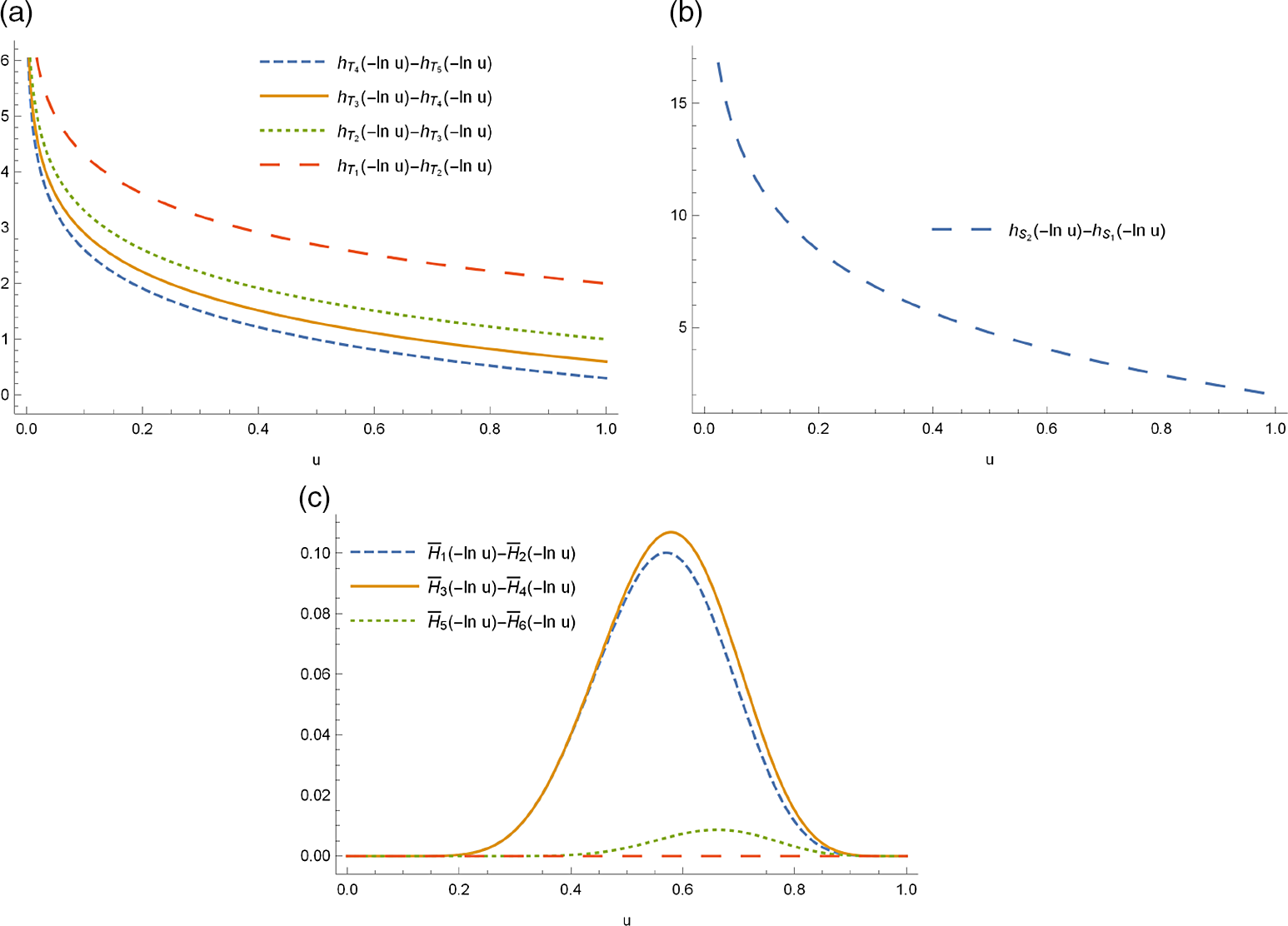
From the plots in Figures 8(a) and 8(b) we can see that
 $T_1\le_{hr}T_2\le_{hr}T_3\le_{hr}T_4\le_{hr}T_5 $
and
 $S_1\ge_{hr} S_2 $
. Meanwhile, Figure 8(c) plots the difference functions
 $\overline H_{i}(t)-\overline H_{i+1}(t) $
, for
 $i=1,3, 5$
, where
 $t=-\ln u$
and
 $u \in [0,1]$
, from which it is clear that all difference functions are non-negative. Thus the relevation redundancy should be put to the node having the weakest component with lifetime
 $T_2$
within the minimal path set
 $P_4 = \{2,3,4\}$
, which is in accordance with the theoretical result of Theorem 4.
(a) Plots of the difference function
 $h_{T_{i}}(-\ln u)-h_{T_{i+1}}(-\ln u)$
for
 $i=1,\ldots,4$
and
 $u\in[0,1]$
. (b) Plot of the difference function
 $h_{S_{2}}( -\ln u)-h_{S_{1}}( -\ln u)$
and
 $u\in[0,1]$
. (c) Plots of the difference function
 $\overline H_{ i}( -\ln u) - \overline H_{ i+1}( -\ln u)$
for
 $i=1,3,5$
and
 $u\in[0,1]$
.

For the case of load-sharing and minimal repair policies, the following results can be obtained directly from Theorems 2 and 3 for coherent systems.
Proposition 3. In the set-up of Theorem 4, let
 $\tau_1$
and
 $\tau_2$
be the resulting system lifetimes with common structure function
 $ \Phi $
under two different load-sharing models
 \begin{equation*} T_1,\ldots, T_{i-1}, T_{i, L/\alpha}\#T_i, T_{i+1}, \ldots, T_j , \ldots, T_n\end{equation*}
and
 \begin{equation*} T_1, \ldots, T_i, \ldots, T_{j-1}, T_{j, L/\alpha}\#T_j, T_{j+1}, \ldots, T_n,\end{equation*}
respectively. Then the condition
 $\gamma_{T_i}(t) \le \gamma_{T_j}(t)$
for all
 $t\in\mathbb{R}_+$
implies that
 $\tau_1 \ge_{hr} \tau_2$
.
Proposition 4. In the set-up of Theorem 4, let
 $\tau_1$
and
 $\tau_2$
be the resulting system lifetimes with common structure function
 $ \Phi $
under two different minimal repair policies
 \begin{equation*} T_1,\ldots, T_{i-1}, T_i\#S_1, T_{i+1}, \ldots, T_{j-1},T_j , T_{j+1}\ldots, T_n\end{equation*}
and
 \begin{equation*} T_1, \ldots, T_{i-1}, T_i , T_{i+1}, \ldots, T_{j-1}, T_j\#S_2, T_{j+1}, \ldots, T_n,\end{equation*}
respectively. Then the condition
 $\beta_{T_i}(t) \ge \beta_{T_j}(t)$
for all
 $t\in\mathbb{R}_+$
implies that
 $\tau_1 \ge_{hr} \tau_2$
.
4. Conclusion
In this work we have studied the allocations of relevations in coherent systems. In particular, we have studied the problem of allocating one or two relevations to improve the reliabilities of series systems in the sense of the usual stochastic ordering and the hazard rate ordering. These results are further generalized to the case of coherent systems. Further research might focus on the study of allocations of more than two relevations in coherent systems with dependent components. Another problem of interest is to generalize Theorem 4 when the components belong to two different disjoint sets, as mentioned in [Reference Belzunce, Martnez-Riquelme and Ruiz7].
Acknowledgements
The authors thank the insightful and helpful comments and suggestions from an Editor and two anonymous reviewers, which have greatly improved the presentation of the paper. The authors are ranked in alphabetic order. Rongfang Yan and Jiandong Zhang acknowledge financial support of the National Natural Science Foundation of China (no. 11861058 and no. 71471148). Yiying Zhang acknowledges the National Natural Science Foundation of China (no. 12101336), and the Natural Science Foundation of Tianjin (no. 20JCQNJC01740).