Nomenclature
- AGCNN
-
attention-based gated convolutional neural network
- AI
-
artificial intelligence
- ANFIS
-
adaptive neuro-fuzzy inference system
- ANN
-
artificial neural network
- AR
-
autoregressive model
- BGRU
-
bidirectional gated recurrent units
- CART
-
classification and regression tree
- C-MAPSS
-
Commercial Modular Aero-Propulsion System Simulation
- CNN
-
convolutional neural network
- CONV-LSTM
-
convolutional neural networks with long short-term memory
- CONV-MLP
-
convolutional neural networks and multi-layer perceptron
- CONV1D
-
one-dimensional convolutional neural network
- CPU
-
central processing unit
- DT
-
decision tree
- EN
-
elastic net
- FLS
-
fuzzy logic system
- GPU
-
graphics processing unit
- LSTM
-
long short-term memory
- MAE
-
mean absolute error
- MLP
-
multi-layer perceptron
- PdM
-
predictive maintenance
- PHM
-
prognostic and health management
- PSO
-
particle swarm optimisation
- RF
-
random forests
- RMSE
-
root mean square error
- RNN
-
recurrent neural network
- RUL
-
remaining useful life
- RVM
-
relevance vector machine
- RVR
-
relevance vector regression
- SQP
-
sequential quadratic optimisation
- SVR
-
support vector regression
- XGB
-
eXtreme Gradient Boosting
1.0 Introduction
Monitoring the health state and optimising the service life of industrial machines is a major concern in the field of prognostic and health management (PHM). Hence, the main objective of PHM is to accurately predict future machine failures, mainly by estimating their remaining useful life (RUL). With the advent of the fourth industrial revolution, PHM methods employ artificial intelligence (AI) methods, notably machine learning techniques, using monitoring data to anticipate the RUL of industrial machines. Actually, these techniques offered accurate predictions in several research works [Reference Wang, Zhao and Addepalli1]. However, they suffer mainly from their inability to take into account imprecise data, since data sources are generally not totally reliable. Besides, a major challenge in this field is that RUL predictions could considerably vary from one AI learning method to another, compromising their reliability. We cannot, therefore, affirm their high reliability for all types of monitoring data.
Since this variation is largely due to the imprecision of the data used to drive the models, our aim in this work is to carefully study the influence of sliding time window process on prediction results by an exemplary protocol while implementing a RUL prediction process that takes advantage of various AI models, including long short-term memory (LSTM), convolution neural networks (CNN) and multi-layer perceptrons (MLP). These algorithms perfectly handle knowledge extraction from complex time series patterns. In addition, to refine the prediction of the above-mentioned methods, we put in place an ensemble learning strategy. It aggregates the aforementioned deep learning methods while addressing the problem of data imprecision and handling uncertainty on complex datasets.
To this end, the decision tree (DT) on the one hand, and adaptive neuro-fuzzy inference systems (ANFIS) [Reference Jang2] on the other hand, are considered as meta learners to implement ensemble learning. Actually, ANFIS has been applied in several fields, especially within the predictive maintenance (PdM) [Reference Zhao, Chen, Guo and Li3–Reference Meddour, Messekher, Younes and Yallese7]. In this paper, ANFIS and a decision tree are integrated into a process integrating other tools of preprocessing and learning with a special focus on turbofan engines’ application, referring to as the commercial modular aero-propulsion system simulation (C-MAPSS) dataset [8]. In aeronautic domain, engine maintenance is highly important and critical, and monitoring engine health and degradation can highly impact the maintenance of the engine. In this work, the models are trained and assessed on engine degradation trajectories, considering operating regimes and degradation phases. Ensemble learning profiting from the ANFIS algorithm is able to manage the imperfection inherent in monitoring data and allowing more accurate results.
The rest of this paper is organised as follows. Section 2 reviews related works in the PdM field, which are also using machine and deep learning and/or tackling the problem of data imperfection, with a special focus on those using neuro-fuzzy learning. The theoretical aspects of the ANFIS algorithm are, then, introduced in Section 3. Section 4 is dedicated to detailing our proposal, addressed to turbofan engines, to accurately estimate RULs using deep learning and ANFIS methods. Section 5 is devoted to presenting our experimental analysis, comparative study and discussion. Finally, we conclude in Section 6.
2.0 Related work
In the field of PHM, the literature has witnessed a widespread focus on RUL prediction. Research approaches in the literature could be classified in different ways. The most recently used way is to categorise them into physics-based approaches, which refer to physical failure techniques, data-driven approaches or hybrid-data approaches [Reference Wang, Zhao and Addepalli1]. The main strength of data-driven approaches is that they do not require an empirical estimation of physics parameters or prior knowledge from experts to predict the RUL, which makes them quickly implemented and deployed. For instance, in the investigation by Ref. [Reference Alabadi and Habbal9], the authors implemented novel decentralised techniques with deep learning techniques to accurately predict the RUL. The authors proved that the accuracy of prediction is improved. They used the C-MAPSS dataset and LSTM as deep learning methods. In a similar investigation [Reference Liu, Zhang, Guo, Bian, He and Liu10], the authors apply Bi-LSTM instead to improve the predicted model. In another work by Ref. [Reference Sateesh Babu, Zhao, Li, Navathe, Wu, Shekhar, Du, Sean Wang and Xiong11], the authors applied another type of deep learning to predict RUL. The authors believe that algorithms, like MLP, are not able to learn from patterns of features in this domain, solely. They used CNN as a deep neural network algorithm to predict the RUL, along with C-MAPSS as a data set. They demonstrate that the predictive performance is enhanced compared to models based on algorithms such as MLP, support vector regression (SVR) and relevance vector regression (RVR). In order to improve the performance of the LSTM model on the C-MAPSS dataset, the authors of Ref. [Reference Asif, Haider, Naqvi, Zaki, Kwak and Islam12] put efforts into developing the preprocessing stage. They combined the deep learning algorithm with a dimensionality reduction algorithm and a piecewise linear RUL function. In a similar work by Ref. [Reference Hong, Lee, Lee, Ko, Kim and Hur13], authors combine several deep learning algorithms (bidirectional LSTM, LSTM and CNN) with dimensionality reduction to improve the performance of predictions. Authors of Ref. [Reference Li, Wang, Wang, Ma, Miao, Xu and Cheng14], like the abovementioned works, combine different methods to obtain better performance. They use the Savitzky-Golay filter to improve data preprocessing. Then, they leverage the feature extraction capabilities of CNN and combine them with LSTM networks to model temporal dependencies in the data. Their results show that this hybrid architecture outperforms similar approaches in terms of predictive performance. In an investigation by Ref. [Reference Liu, Liu, Jia and Lin15], a method named feature-attention-based bi-directional gated recurrent unit convolutional neural network (AGCNN) is proposed. The input data is first weighted using a feature-attention mechanism. Then, a combination of bi-directional gated recurrent units (BGRU) and CNN is employed to extract relevant temporal and spatial features. Finally, a fully connected network completes the learning process by performing the final prediction. The researchers in Ref. [Reference Mo, Lucca, Malacarne and Iacca16] also leveraged the strengths of both LSTM and CNN architectures to enhance the performance of their predictive model built on the C-MAPSS dataset. The proposed data-driven algorithms could be straightforwardly adapted and used for other types of systems. The idea is to handle and study historical/monitoring data to predict the health state of systems. In most investigations, authors tried to use various types of algorithms and combine them with preprocessing techniques like dimensionality reduction or a piecewise linear function. However, sliding window techniques on time series data, like C-MAPSS, play a crucial role that has not been rigorously explored in this domain on the C-MAPSS dataset. In addition, data-driven approaches have also been classified by authors, in [Reference An, Kim and Choi17], into two main sub-categories: AI approaches and statistical approaches. However, the primary limitation of such approaches lies in the algorithm’s necessity to exhibit robustness. To do so, we should manage uncertainty/imprecision inherent within data, which could be due to data sources’ reliability, and boost prediction performance by applying robust techniques, such as ensemble learning.
2.1 Ensemble learning for prediction
Ensemble learning methods consist of measurement algorithms that merge several basic learners to form a single predictive model, with the aim of improving prediction performance [Reference Li, Wu, Hu and Terpenny18]. The three most common techniques of ensemble learning are: bagging, boosting and stacking [Reference Schwinger19].
-
• Bagging involves training multiple models on samples obtained by bootstrapping and combining their predictions by majority vote (for classification tasks) or mean (for regression tasks).
-
• Boosting involves the sequential training of several weak models with increased attention paid to misclassified examples at each stage.
-
• Stacking involves training several base models on the entire data set, whose predictions serve as input features for a meta-learning model that aggregates these predictions.
Actually, ensemble learning methods fall into two categories: parallel and sequential. Parallel methods, such as random forests (RF), construct several basic learners independently, and then aggregate their predictions by taking the weighted mean or sum. These methods can be implemented using uncertainty management frameworks, where weights are interpreted as probabilities, such as in Ref. [Reference Li, Goebel and Wu20]. In contrast, sequential methods, such as AdaBoost, build base learners sequentially to reduce the bias of combined learners, where imprecision could be managed inside one of the used learners. The investigators in Ref. [Reference Li, Goebel and Wu20] developed a predictor model to estimate RUL by ensemble learning utilising the C-MAPSS dataset. They profited from RF, classification and regression tree (CART), recurrent neural network (RNN), autoregressive model (AR), ANFIS, relevance vector machine (RVM) and elastic net (EN) as basic predictors. Particle swarm optimisation (PSO) and sequential quadratic optimisation (SQP) are used to determine the optimum weights of basic learners. The authors illustrated that the performance of predictors increased compared to other works. The authors, in Ref. [Reference Ture, Akbulut, Zaim and Catal21], implement stack ensemble learning on the C-MAPSS dataset to predict the RUL. They propose five different regression algorithms (DT regression, SVR, linear regression, RF regression and extreme gradient boost regression) to develop stack ensemble learning. They proved that the accuracy of prediction is improved using stacked ensemble learning. In Ref. [Reference Zhang, Xiao, Yang, Cheng, Chen, Gao, Liu and Huang22], authors propose, also, an ensemble learning method taking advantage of CNN and eXtreme Gradient Boosting (XGB) algorithms and averaging aggregation to predict the RUL. They show that using ensemble learning yields better results than relying on CNN alone. Applying ensemble learning methods shows promising results for improving the performance of prediction models in this domain. It allows us to profit from the power of different algorithms to construct more robust models. However, given the wide range of algorithms, their potential combinations and the variety of implementation strategies, extensive research is still required to explore the full potential of ensemble learning. In this context, a key challenge lies in the ability of models not only to deliver accurate predictions but also to quantify the uncertainty associated with them.
2.2 Managing uncertainty for RUL prediction
Predicting the RUL while managing data imperfections is a key challenge in the field of PdM and PHM. Traditional prediction systems often come up against noisy, incomplete or imprecise data, which can lead to unreliable predictions. To overcome these problems, advanced approaches such as the use of AI models, including LSTM, neural networks and MLP, along with uncertainty management approaches, have been developed. As an example, in Ref. [Reference Ayed, Broujeny and Tahar Hamza23], an evidential multi-layer perceptron model is developed to quantify uncertainty in data and predictions. These models are capable of processing complex data and capturing non-linear patterns. In particular, fuzzy learning techniques, such as ANFIS, detailed in the following section, are applied to deal with data imperfection. For instance, the study presented in Ref. [Reference Tavakoli, Najafi and Sharifara24] employs ANFIS to predict the RUL of water pipes in a distribution system, while also identifying the key parameters that influence these predictions. In addition, ANFIS has been embedded, in Ref. [Reference Wu, Su, Cheng, Shao, Deng and Liu25], within a feature fusion and a RUL prediction method. The latter work proposes a schematic representation of a multi-sensor information fusion system for the online RUL prediction of machining tools. Ultimately, we note in Ref. [Reference Hadroug, Hafaifa, Iratni and Guemana26] that ANFIS has been used in the same field to model the reliability, availability and durability of gas turbines through their monitoring data and failure assessment indicators.
Previous studies have demonstrated the use of advanced techniques such as ANFIS to manage the uncertainty inherent in predictive maintenance data, offering a promising alternative by combining the strengths of neural networks and fuzzy logic systems. Building on this foundation, the present work proposes a novel ensemble learning approach for RUL prediction that explicitly integrates uncertainty management through ANFIS. The originality of this work lies in both the combination of hybrid learners and the exploration of temporal structures, specifically the effect of sliding window sizes, on predictive performance. In the first phase, we assess the performance of simple learners combining CNN with MLP, and CNN with LSTM, to establish baseline behaviours. We then introduce a more sophisticated ensemble model that leverages ANFIS and DT as meta-learners, aiming to improve robustness and interpretability. This approach not only enhances prediction accuracy but also contributes to a better understanding of model uncertainty, an essential aspect for real-world deployment in industrial contexts. The following section presents the ANFIS architecture and discusses its contribution to uncertainty-aware RUL prediction.
3.0 Adaptive neuro fuzzy inference system
ANFIS system is a machine learning based that combines the principles of fuzzy logic and neural networks. It is a hybrid system, combining artificial neural network (ANN) and fuzzy logic system (FLS), designed to capture complex fuzzy relations using neural networks while exploiting the structure of fuzzy rules. The adaptive neuro-fuzzy inference system [Reference Azar27, Reference Dong and Wang28] is based on the systematic creation of fuzzy rules, using the Takagi-Sugeno inference model [Reference Camargos, Bessa, D’Angelo, Cosme and Palhares29, Reference Chen, Liu, Chen and Zhang30]. It improves on pre-existing fuzzy rules defined by human experts by adjusting the overlap between sets of fuzzy rules describing the input-output behaviour of the industrial system under examination, particularly turbofan engines. The standard architecture of the ANFIS algorithm is based on a series of
 ${R_i}$
rules defined by an If-Then relationship. Consider
 ${x_1}$
and
 ${x_2}$
, two linguistic input variables associated with the fuzzy sets
 ${A_1}$
,
 ${A_2}$
,
 ${B_1}$
and
 ${B_2}$
, and the rule base contains the following two types of rules with the outputs
 ${f_1}$
and
 ${f_2}$
:
 \begin{align}& {{R_1}\ :\ If\ {X_1}\ Is\ {A_1}\ and\ {X_2}\ is\ {B_1}\ Then\ {f_1}({{X_1},{X_2}}) = {p_1}{X_1} + {q_1}{X_2} + {r_1}} \nonumber\\[6pt]& {R_2}\ :\ If\ {X_1}\ Is\ {A_2}\ and\ {X_2}\ is\ {B_2}\ Then\ {f_2}( {{X_1},{X_2}}) = {p_2}{X_1} + {q_2}{X_2} + {r_2} \end{align}
Then, the outputs of the defuzzification neurons depend on the consequence parameters of the rule, namely
 ${p_i}$
,
 ${q_i}$
and
 ${r_i}$
, which are set during the learning process.
As presented in Fig. 1, ANFIS has an architecture consisting of five layers: in the first layer, the input variables are mapped to the membership degrees using membership functions in each node,
 \begin{align}O_1^i = {\mu _{{A_i}}}\left( x \right),{\rm{\;\;\;\;}}i = 1,2 \\[-28pt] \nonumber \end{align}
 \begin{align}O_1^i = {\mu _{{B_{i - 2}}}}\left( y \right),{\rm{\;\;\;\;}}i = 3,4 \\[0pt] \nonumber \end{align}
where
 ${\mu _A}$
and
 ${\mu _B}$
represent the membership functions.
ANFIS structure [Reference Wu, Su, Cheng, Shao, Deng and Liu25, Reference Haznedar and Kalinli31].

In the second layer, each node refers to a rule that is generated by the fuzzy system. It represents the firing strength for the rules generated in the fuzzification step.
 \begin{align}O_2^i = {w_i} = {\mu _{{A_i}}}\left( x \right){\rm{*}}\,{\mu _{{B_i}}}\left( y \right),{\rm{\;\;\;\;}}i = 1,2 \end{align}
The third layer normalises the firing strength for each input.
 \begin{align}O_3^i = {\bar w_i} = \frac{{{w_i}}}{{{w_1} + {w_2}}},{\rm{\;\;\;\;}}i = 1,2 \end{align}
The fourth layer is simply the defuzzification. It is a product of the normalised firing and a polynomial function to calculate out put of each node.
 \begin{align}O_4^i = {\bar w_i}\cdot{f_i} = {\rm{\;\;}}i = 1,2 \end{align}
Finally, in the fifth layer, where there is only one node, the sum of output nodes is calculated by a summation.
 \begin{align}O_5^i = f = \sum \bar{w}_{i}\cdot{f_i} = {\rm{\;\;}}i = 1,2 \end{align}
ANFIS performs its learning by adjusting its adaptive parameters, such as
 $\left\{ {{p_i},{q_i},{r_i}} \right\}$
, with the aim of minimising the deviation between the actual and desired output. The standard ANFIS learning process, performed in two passes, combines gradient descent and a least squares estimator. On the one hand, the least-squares estimator updates the consequent parameters in the forward pass. On the other hand, the basic parameters are adjusted in the back pass by the gradient descent method, using the back-propagation technique.
This method is integrated within a process that we present in the following section, to study the health state of turbofan engines through their monitoring data.
4.0 Turbofan engines RUL prediction with imprecision management and ensemble learning
Our proposed strategy consists of two phases and three levels, as presented in Fig. 2. The first phase (pre-processing) consists of Level 1, and the second phase consists of Levels 2 and 3 (training and ensemble learning).
Actually, our model could be adapted and applied to different kinds of industrial machinery once we have monitoring data available. However, we are focusing, in this work, on the aeronautic field, particularly on aircraft engines and the C-MAPSS dataset.
4.1 Monitoring data: C-MAPSS dataset presentation
C-MAPSS [8] presents a monitoring database of aeronautical systems. It was mainly created for the competition ‘Prognostics Center of Excellence’ of NASA and then used by various research works to propose and develop diagnostic and prognostic algorithms for aircraft engines. As we can conclude, the C-MAPSS dataset focuses on aircraft engines, in particular jet engines. It is designed to reflect the complexity of commercial aircraft propulsion systems. It simulates various engine degradation and aging scenarios, which allows for analysing and developing predictive maintenance models based on these conditions.
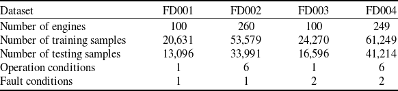
C-MAPSS data subsets in detail [8, Reference Hong, Lee, Lee, Ko, Kim and Hur13]

The proposed process for RUL ensemble learning.

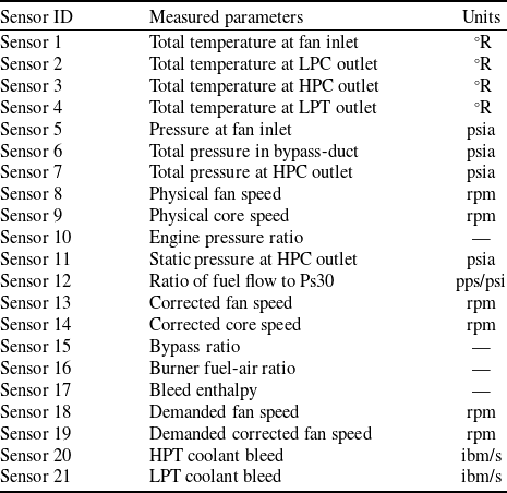
Moreover, C-MAPSS contains detailed records of several motor operating parameters (or sensors), such as temperatures, pressures, and rotational speeds. This data is crucial for the analysis and development of predictive maintenance models, as well as for analysing motor behaviour. C-MAPSS dataset includes four different subsets, named FD001, FD002, FD003 and FD004. Each subset of the train set data and test set data is presented separately. Each subset is set differently in terms of engine operation condition, failure type and engine numbers. In this study, we considered subset FD004. Table 1 illustrates the C-MAPSS dataset and its subsets in detail. The details regarding sensor measurement are presented in Table 2 and Fig. 3. There are 21 sensory data and 3 operational settings columns in the dataset.
Sensor details in the C-MAPSS dataset [8, Reference Hong, Lee, Lee, Ko, Kim and Hur13]

Schema of turbofan engine regarding C-MAPSS dataset [Reference Frederick, DeCastro and Litt32].

4.2 Phase I: preprocessing
Phase I is included in just one level. As preprocessing, two distinct approaches exist for predicting the RUL [Reference Goebel, Saha, Saxena, Mct and Riacs33]. The first one involves straightly aligning the data with the RUL, while the alternative approach focuses on examining the degradation process of the motor. In the latter method, the degradation process is analysed, and a correlation is established between the degradation process and the RUL, which is mainly the purpose of our pre-processing step. Hence, we need to define a health index, followed by extracting relevant features from this index. These extracted features play a crucial role in the prognostic procedure. This phase is, therefore, composed of different steps that should be executed before moving on to the learning phase.
4.2.1 Feature selection
Feature selection constitutes a crucial phase in examining data derived from the simulation of the C-MAPSS dataset. Given the intricate nature of data stemming from simulations of aircraft propulsion systems, it is essential to identify the most relevant attributes for developing effective predictive models. In this study, our primary focus has been on reducing uninformative attributes, aiming to decrease the dimensionality of the data. Feature selection was carried out using two different approaches: (1) feature importance score by a DT and (2) plotting-visualisation analysis of sensors versus RUL. In the first step, feature importance is calculated by a DT on random motors. It presents the features with a score that indicates their participation in the learning process. Figure 4 illustrates the feature importance scores on two chosen random motors. As an example, sensors 3, 4, 8, 13, 19, 21, 22 have low scores, and they are removed. However, the evolution of each sensory data versus RUL is checked to aggregate the final decision. In some cases, despite a low score of feature importance, the visualisation recommends keeping the features, and vice versa; despite the high score, the visualisation recommends removing them (due to no visible evolution of sensory data versus RUL). In most cases, the visualisation of sensory data versus RUL is in accordance with feature importance scores.
Comparison of feature importance scores between engine 34 and engine 117.

As some examples, Figs 5 and 6 illustrate the plots on engines 34 and 117, and data from sensors 7 and 12. As these two figures illustrate, the parameters of the selected sensors are sensitive to RUL, and they illustrate an increment following the fall of the RUL. This graphical approach enables us to visualise the relation between RUL and sensory data. Based on these visualisations, we identify the sensory data that are sensitive to degradation and RUL. Consequently, the attributes without significant fluctuations (sensitivity to RUL) have been removed from the analysis in order to simplify the model and improve its efficiency. According to this approach, features 1, 2, 3, 4, 8, 9, 19, 21 and 22 are eliminated. They are the features with low feature importance scores and no visible variations during the life cycle of engines.
Sensor 7 fluctuations during the RUL of engines 34 and 117.

Sensor 12 fluctuations during the RUL of engines 34 and 117.

Figure 6 Long description
Panel A: A scatter plot depicts Sensor 12 variations versus Remaining Useful Life (RUL) of engine 34. The horizontal axis represents RUL with values ranging from 0 to 300, and the vertical axis represents Sensor 12 Value with values ranging from 8000 to 9000. The plot includes green data points connected by green lines, showing fluctuations in Sensor 12 values. Two red horizontal lines are present, one around 8400 and the other around 8800, likely indicating thresholds or boundaries. Panel B: A scatter plot depicts Sensor 12 variations versus Remaining Useful Life (RUL) of engine 117. The horizontal axis represents RUL with values ranging from 0 to 350, and the vertical axis represents Sensor 12 Value with values ranging from 8000 to 9000. Similar to Panel A, this plot includes green data points connected by green lines, showing fluctuations in Sensor 12 values. Two red horizontal lines are present, one around 8400 and the other around 8800, likely indicating thresholds or boundaries.
4.2.2 Normalisation
In this pre-processing stage, normalisation is carried out using the min-max normalisation method. This technique involves resizing the values of each attribute to bring them within the range [0, 1]. For every value
 $X$
in an attribute, its normalisation
 ${X_{norm}}$
is calculated as follows:
 \begin{align}{X_{norm}} = \frac{{X - {X_{min}}}}{{{X_{max}} - {X_{min}}}} \end{align}
where
 ${X_{min}}$
and
 ${X_{max}}$
refer respectively to the minimum and maximum values of the attribute.
The benefit of this approach lies in its ability to maintain the distribution of the data while adjusting it to a common scale, thus facilitating comparison and analysis of the various features. For C-MAPSS data, min-max normalisation ensures data homogeneity, thus promoting variable consistency, an essential consideration for the development of robust predictive maintenance models.
4.2.3 Data cleaning and labeling based on piece-wise function
In this step, we focused on data preparation by standardising the degradation starting point across all engines. To standardise the C-MAPSS dataset and streamline the modeling process, we adopt the assumption that the RUL remains constant at 125 for an initial phase during which no degradation occurs, and that degradation begins consistently from RUL = 124 onward. This assumption simplifies the labeling procedure and reduces inter-engine variability, thereby contributing to more consistent and reliable model training. By fixing the degradation onset point, the dataset becomes more homogeneous across engines, which facilitates the learning process and improves the generalisation capabilities of predictive models.
Application of a piecewise function
After segmenting the data into ‘normal’ and ‘degradation’ phases, we apply a piecewise function to model the engine’s performance more effectively. A piecewise linear function is used to represent the engine’s operational phases, with the first segment corresponding to normal functioning and the second segment capturing the degradation phase.
The idea is to simplify the complex nonlinear behaviours exhibited by engines into manageable linear segments. By doing so, it enhances the accuracy of the RUL predictions and provides a clearer understanding of the engine’s degradation trajectory.
Data labeling
To optimise the dataset for learning models, we labeled each cycle according to its phase (normal or degradation) and calculated the RUL for each cycle. During the normal phase, the RUL is calculated as the total remaining cycles until failure. In the degradation phase, the RUL decreases more rapidly, reflecting the engine’s accelerated wear.
4.2.4 Time delays configuration
With the data now labeled, the next critical challenge is handling the inherent delays in the sequential data, especially in time series datasets. Addressing these delays is essential for improving the model’s ability to accurately capture temporal dependencies in the data. To examine the influence of sliding windows, and to discover the optimised value of the sliding window (time delay of prediction), 30 different datasets are generated according to 30 different numbers of sliding windows between 1 and 30. These 30 datasets serve as part of the investigation for model selection. In the following section, we discuss how we manage these delays through a careful selection process using a sliding window technique.
4.3 Phase II: our proposed process for training and ensemble learning
In this second phase, we present our novel multi-level ensemble training process, designed to systematically combine multiple learning algorithms across different temporal configurations. For each of the 30 sliding window sizes, we train and evaluate several base models (Level 1), including combinations such as CNN-MLP and CNN-LSTM. Each configuration is trained and tested 10 times to account for variability due to random initialisation in neural networks, ensuring statistically robust outcomes.
To further enhance predictive performance, we implement a Level 2 meta-model based on ensemble learning, where ANFIS and DT are employed as meta-learners. These learners aggregate the predictions of the base models while integrating uncertainty information. In total, this approach results in the generation and evaluation of over 1,200 models, excluding hyperparameter optimisation steps, making our process one of the most exhaustive comparative evaluations in this domain.
By exhaustively exploring the effects of time delays, model diversity and ensemble configurations, our method aims not only to improve accuracy but also to increase robustness and reliability in RUL prediction. The following sections detail the learning strategies implemented in Levels 2 and 3 of our proposed architecture.
4.3.1 Level 2: considered deep learning methods for RUL prediction
At Level 1 of our approach, we implement deep learning methods dedicated to the RUL prediction. We are exploring the use of advanced techniques such as deep neural networks, which are specifically designed to capture complex patterns in temporal data. The aim is to exploit the ability of deep neural networks to extract meaningful features from temporal sequences, thereby improving the accuracy of RUL predictions. As mentioned in Fig. 2, we particularly use the hybrid architectures, CONV-MLP [Reference Li, Hassani, Walton and Shi34] on the one hand, and CONV-LSTM [Reference Shi, Chen, Wang, Yeung, Wong and Woo35] on the other hand.
-
• CONV-MLP: The combination of CNN and MLP has been employed to effectively model and predict complex time series data. In this approach, CNNs are leveraged to automatically extract relevant spatial features and patterns from the input data by applying convolutional filters, which help capture local dependencies. These extracted features are then passed to the MLP, which is responsible for modeling the nonlinear relationships between these features and the target variable in a supervised learning framework. By combining CNN’s feature extraction capabilities with MLP’s strength in nonlinear mapping, the CONV-MLP model can handle both spatial and temporal complexities in the data, leading to improved prediction accuracy. In this study, we specifically used a one-dimensional CNN (CONV1D) model to process the time-series data, focusing on temporal feature extraction.
-
• CONV-LSTM: While the CONV-MLP model combines CNN and MLP to handle spatial and temporal complexities, the CONV-LSTM model extends this approach by integrating CNN with LSTM networks, which are particularly effective for capturing long-term dependencies in sequential data. In this architecture, CNNs are responsible for extracting spatial features from the input data, similarly to the CONV-MLP model. However, instead of using an MLP for further processing, the LSTM network takes over to model the temporal dynamics, using its internal memory to capture long-term dependencies and patterns in the time series data. This approach is especially advantageous when time-related dependencies span longer sequences, as LSTMs are designed to retain and update relevant information across time steps. For this work, we utilised a CONV1D model, which is tailored to extract both temporal and spatial features from the time-series data, enhancing the model’s ability to predict complex sequences with greater accuracy.
4.3.2 Level 3: comparing fuzzy and hard learning using deep neural networks’ predictions
At Level 3 of the second phase, we focus on an in-depth analysis comparing two distinct approaches: fuzzy learning and strict learning. This step leverages the capabilities of deep neural networks, which are complex models specifically designed to process temporal data. The aim of this comparison is to assess the effectiveness of these different approaches by confronting fuzzy learning with a more rigorous and structured approach.
We look at how these two paradigms, neuro-fuzzy learning via ANFIS and strict learning via DT, affect the performance of deep neural networks when making RUL predictions. This involves an in-depth analysis of the results obtained, highlighting how each approach impacts the model’s ability to accurately anticipate remaining component life. This dual-meta-learning strategy is particularly original in that it contrasts two fundamentally different reasoning mechanisms, one based on human like fuzzy inference (ANFIS), and the other on rule-based, deterministic structures (DT), offering complementary perspectives on uncertainty handling and interpretability in ensemble learning.
The ultimate aim of this comparison is to determine which method is best suited to our specific context. We seek to identify the one that offers optimal results in terms of accuracy and reliability of RUL predictions. By discerning the strengths and weaknesses of each approach, we will be able to steer our choice towards the most relevant method for the specific needs of our study, thus contributing to improving the overall performance of our ensemble learning model.
5.0 Experimental analysis
We aim, during this section, to conduct an experimental study and assess the four sets of predictions, dispatched on two levels, as already mentioned in Fig. 2.
-
• Level 2: Simple learning
-
- Predictions 1: Via CONV-MLP
-
- Predictions 2: Via CONV-LSTM
-
-
• Level 3: Ensemble learning
-
- Predictions 3: Via the stacking technique of ensemble learning
-
* Meta-learning model by DT: META-DT
-
* Base models: CONV-MLP and CONV-LSTM
-
-
- Predictions 4: Via the stacking technique of ensemble learning
-
* Meta-learning model by ANFIS: META-ANFIS
-
* Base models: CONV-MLP and CONV-LSTM
-
5.1 Evaluation criteria
To measure the accuracy of the different generated predictions, we call the root mean square error (RMSE) criterion, the mean absolute error (MAE) and the coefficient of determination (
 ${R^2}$
). They represent the error rate between model prediction and actual values. Another criterion, as an evaluation metric, is implemented: it is a function that scores the prediction for each learning algorithm; the score value (S) is sensitive to overestimation or underestimation of prediction, and it is widely used in this domain [Reference Saxena, Goebel, Simon and Eklund36]. RMSE is calculated such that:
 \begin{align}RMSE = \sqrt {{1 \over n}\mathop \sum \limits_{i = 1}^n {{({y_i} - {{\hat y}_i})}^2}} \end{align}
where
 ${y_i}$
represents the observed or actual value,
 ${\hat y_i}$
corresponds to the value predicted by the model and
 $n$
is the total number of observations.
The MAE and
 ${R^2}$
are calculated as follows, where
 $\bar y$
is the average of actual values:
 \begin{align}MAE = {1 \over n}\mathop \sum \limits_{i = 1}^n \left| {{y_i} - {{\hat y}_i}} \right| \\[-28pt] \nonumber \end{align}
 \begin{align}{R^2} = 1 - {{\mathop \sum \nolimits_{i = 1}^n {{({y_i} - {{\hat y}_i})}^2}} \over {\mathop \sum \nolimits_{i = 1}^n {{({y_i} - \bar y)}^2}}} \\[0pt] \nonumber \end{align}
The score is calculated as follows:
 \begin{align}S = \begin{cases} {\mathop \sum \nolimits_{i = 1}^n \big( {{e^{ - {{{d_i}} \over {13}}}} - 1} \big),} & {}{{\rm{if}}\ {d_i} \lt 0,} \\[6pt] {\mathop \sum \nolimits_{i = 1}^n \big( {{e^{{{{d_i}} \over {10}}}} - 1} \big),} & {}{{\rm{if}}\ {d_i} \ge 0.} \end{cases} \end{align}
where
 ${d_i} = {\hat y_i} - {y_i}$
.
5.2 Parameters settings
In this section, we detail the configuration of the parameters used in our experiments. The experimental setup was conducted on the subset FD004 of C-MAPSS. The configuration of the parameters for each predictor is discussed in detail, including the selection of key hyperparameters such as the number of layers, time delays and membership functions used for the META-ANFIS model. In addition, it should be mentioned that all experiments are done using the local server of our laboratory. The server is equipped with Windows 10 (64-bit), a 12-core CPU, an NVIDIA T4 GPU with 16 GB of VRAM and 32 GB of system RAM. We used the Spyder as an integrated development environment using Python with TensorFlow GPU support.
5.2.1 Data partitioning, identification of different sets and experimental setup
The available data are divided into three distinct sets: training, validation and test sets. The training set is used to optimise the model parameters, while the validation set serves for hyperparameter tuning. The test set is reserved for evaluating the final model performance. Specifically, the training portion of the FD004 subset is split into 80% for training and 20% for validation. In the next stage, the test set of FD004 is used to assess the model’s predictive performance across all engines. For visualisation purposes, six engines (engine 47, engine 69, engine 70, engine 91, engine 143 and engine 202) are randomly selected from the test set. To evaluate and compare the predictive performance of our models, both among themselves and against results from the literature, we focus on the final RUL values predicted for each engine.
5.2.2 Predictor configuration and parameter selection
Four different predictors were used in the experiments, each with specific parameter settings tailored to optimise performance. Parameters were adjusted and fine-tuned for each predictor.
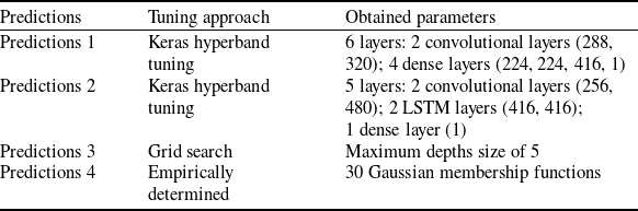
Table 3 provides a summary of the final parameter settings for each predictor. The table specifies the optimal configurations for the number of layers, membership functions and other characteristics depending on the predictor. For Predictions 1 (CONV-MLP), hyperband tuning of the Keras package is used to obtain the parameters of each layer, the same as Predictions 2 (CONV-LSTM). For Predictions 3, which is a DT meta learner, a grid search is applied. Finally, for Predictions 4 (META-ANFIS), both the number and the type of membership functions were determined empirically through experimentation.
Parameters for the four prediction methods

5.3 Results and discussion
This section presents the results of our experiments, focusing on the four RUL predictions generated by different learning strategies, as mentioned in Fig. 2. The models are grouped into two levels of learning: simple learning and ensemble learning. Simple learning includes the CONV-MLP and CONV-LSTM models, while ensemble learning leverages the stacking technique with different meta-learning models.
5.3.1 Performance quantification and model selection based on sliding windows results
As mentioned earlier, 300 models are constructed by each learning algorithm based on different time windows to identify the most optimised sliding windows and, consequently, the best-performing model according to its RMSE. Figures 7, 8, 9 and 10 illustrate the boxplots of RMSE for each sliding window and each learning algorithm. Across all four algorithms, a sliding window size of 28 yields the lowest RMSE, indicating it as the optimal time delay. When considering the median value of each boxplot as a reference for quantifying model performance, the results show that prediction accuracy is relatively poor with smaller window sizes, gradually improves as the window size increases and peaks at 28. Beyond this point, the RMSE starts to rise again, suggesting that overly large time delays may introduce noise or reduce the model’s ability to generalise. According to the above-mentioned, sliding window 28 is identified as the optimised value for setting up the number of time delays. In order to compare the performance of each algorithm on delay 28, Figs 11 and 12 are presented. Figure 11 illustrates the RMSE of models on delay 28 by each learning algorithm, where Fig. 12 shows the obtained scores of models on delay 28 by different learning algorithms. We note, from Fig. 11, that META-ANFIS has a better performance considering RMSE. Among the four algorithms evaluated, META-ANFIS outperforms the others by achieving the lowest minimum and median RMSE, considering 10 trained models per algorithm with a delay of 28. Figure 12 presents the lowest minimum score obtained by the META-DT; however, META-ANFIS has the lowest median compared to the others.
Boxplots of RMSEsfrom the grid search on time delays to select an appropriate delay for training (ANFIS). Blue represents the median, and yellow shows the average of each boxplot.

Boxplots of RMSEs from the grid search on time delays to select an appropriate delay for training (DT). Blue represents the median, and yellow shows the average of each box plot.

Boxplots of RMSEs from the grid search on time delays to select an appropriate delay for training (CONV-MLP). Blue represents the median, and yellow shows the average of each box plot.

Boxplots of RMSEs from the grid search on time delays to select an appropriate delay for training (CONV-LSTM). Blue represents the median, and yellow shows the average of each boxplot.

Boxplot of RMSE of models on delay 28 based on different learning algorithms.

Boxplot of scores of models on delay 28 based on different learning algorithms.

The performance of the final selected models using ensemble learning methods (DT and ANFIS) is evaluated based on standard metrics, including RMSE, MAE,
 ${R^2}$
and the score S, applied to the final time steps of the RUL for all engines, following a common practice in studies using the C-MAPSS dataset. The detailed numerical results are presented in the following section.
Figures 13 and 14 illustrate the RUL predictions generated by META-ANFIS and META-DT, respectively. In both cases, the figures demonstrate the effectiveness of the proposed approaches. Their predictive capabilities are further evaluated on six different engines, as shown in Fig. 15, which provides a comparative analysis of RUL predictions across various models. This figure highlights the differences in performance between engines and contrasts the ground truth values with the predictions made by META-DT and META-ANFIS.
Prediction RULs by DT as meta learner.

Prediction RULs by ANFIS as meta learner.

Comparison of prediction models for different engines in terms of RUL.

5.3.2 Performance quantification of approaches on RUL predictions
The RMSE, MAE,
 ${R^2}$
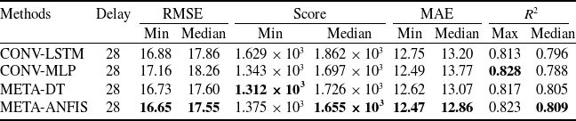
and score results for the RUL predictions across the FD004 dataset are summarised in Tables 4. These predictions are grouped into two levels, each reflecting a different learning complexity. We note that the combination of simple learning models with ensemble learning techniques, particularly the ANFIS-based ensemble, improved RMSE performance across different engines. The careful integration of temporal and spatial features, along with robust uncertainty handling, proved critical in optimising RUL predictions. Table 4 shows the obtained RMSE, MAE, score and
 ${R^2}$
for implemented algorithms and delay number (sliding window) 28.
The ensemble learning models (Predictions 3 and 4) provided notable improvements in RMSE, MAE,
 ${R^2}$
and score by combining the strengths of CONV-MLP and CONV-LSTM with different meta-learning models.
-
• Predictions 3 (stacking with DT): This model delivered balanced error reductions across all tested motors, thanks to the flexibility and interpretability of DT as the meta-learner. The minimum RMSE, MAE and score values are
 $16.73$
,
$12.62$
and
$1.312 \times {10^3}$
, respectively. It has the lowest minimum score among the models. The maximum of
${R^2}$
is 0.82. It shows absolutely better results in the case of RMSE compared to two simple predictors (CONV-MLP and CONV-LSTM). In the case of the lowest minimum scores, it has an advantage over the threes.
-
• Predictions 4 (stacking with ANFIS): The META-ANFIS achieved the best error performance overall (considering RMSE and MAE), excelling in engines with more complex failure modes. It offers the minimum RMSE and MAE values, equal to
$16.65$
and
$12.47$
, respectively. The maximum
${R^2}$
is 0.823, which is slightly lower than 0.828 in CONV-MLP. Regarding the minimum score, it is slightly higher than META-DT; however, it has the lowest median score among all proposed models, which makes it a more interesting choice. Its ability to handle uncertainty and noise contributed to these lowest error values, making it the top-performing model across all four models, despite its slightly lower minimum score compared to META-DT.


5.3.3 Comparison of the proposed approach with the literature review
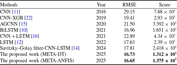
The measured metrics regarding the two proposed meta learners are compared to the investigations of the literature review. Table 5 presents the measured metrics of the proposed approach and other investigations, comparing their RMSE and score values. The investigations are from 2016 to 2025, and they are explained in the literature of our work. The obtained RMSE with META-DT and META-ANFIS shows improvement compared to all proposed works. The closest RMSE to the proposed approach is the work of Ref. [Reference Liu, Zhang, Guo, Bian, He and Liu10]. However, META-DT and META-ANFIS easily outperform it by comparing the score values. They are not only the accuracies of the models slightly better, but also the comparison of scores illustrates, in the case of under- and over-estimation, that the proposed approaches perform better. The investigations of Ref. [Reference Zhang, Xiao, Yang, Cheng, Chen, Gao, Liu and Huang22] are one of the rare examples that used an ensemble learning application in this domain, as explained in the related work. However, the proposed approaches show superior performance compared with this work.
Comparison of RMSE, score, MAE and
 ${R^2}$
for different methods

Comparison of RMSE and score of the proposed work with similar works

6.0 Conclusion
This study has explored a novel approach to improve turbofan engines’ RUL prediction by combining ensemble learning and an ANFIS-based approach. The proposed process, articulated in two distinct phases of pre-processing and learning, enabled a comparison of different predicted RULs (four combinations of AI methods). The pre-processing phase included crucial steps, especially for the C-MAPSS dataset, such as feature selection, normalisation, the piecewise method for data labeling and the use of a sliding window to select the most accurate delay for the used recurrent neural networks. The learning phase implemented a set of powerful techniques, including ensemble learning via ANFIS to manage data imprecision, the hybrid architectures CONV-LSTM networks, CONV-MLP and DT.
Four different sets of results have been obtained, where those offered by the ensemble learning are combined sequentially (CONV-LSTM, CONV-MLP). Ensemble learning methods, ANFIS and DT showed an improvement in the accuracy of RUL prediction, underlining the potential of this hybrid approach. In the case of the performance of predictors, META-ANFIS shows better performance with lower errors (RMSE of 16.65 and MAE of 12.47). The META-DT has a slightly better minimum score (
 $1.312 \times {10^3}$
for META-DT and
 $1.375 \times {10^3}$
for META-ANFIS). However, the median of scores shows an advantage of META-ANFIS (
 $1.726 \times {10^3}$
for META-DT and
 $1.655 \times {10^3}$
for META-ANFIS). In the case of the lower minimum score, it shows that despite the better performance and accuracy of META-ANFIS on prediction, the ensemble learning by META-DT performs slightly better in terms of overestimation. However, a lower median of META-ANFIS promises better overall performance. These advances pave the way for future research and applications in the field of predictive maintenance, enhancing system reliability by enabling proactive failure management. Actually, combining sophisticated pre-processing methods and diversified learning techniques with managing data imprecision offers a promising prospect for tackling the complex challenges associated with RUL prediction in a variety of contexts. As a perspective, we aim, therefore, to study other kinds of uncertainty sources, such as the reliability of sensors, and manage them by varying uncertainty management theories.






 R2