1. Introduction
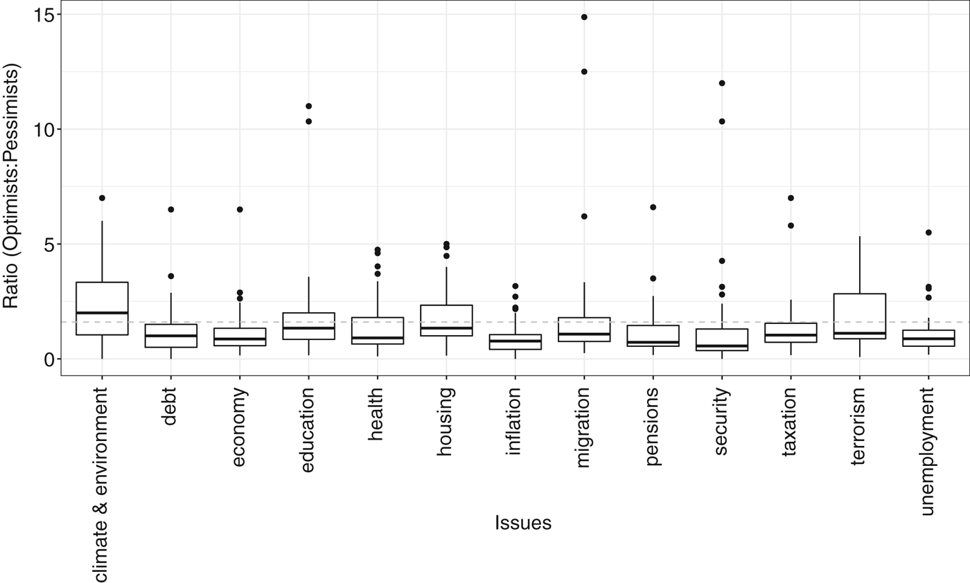
In the absence of technological alternatives, societies with higher ecological preferences support stricter measures to protect the environment. Although this trade-off between pollution and production may be solved in a welfare maximizing manner, the economic performance in such societies may be constrained by stronger regulations and higher taxes. This view is contrasted by our finding that individuals who care a lot about the environment tend to have more optimistic expectations about future economic perspectives. As it can be seen in figure 1, participants in the Eurobarometer 2016 survey who care a lot about the environment are, on average, much more optimistic regarding the economic development of their country compared to any other group of respondents who consider other problems more important. Such influence of positive expectations about the economy runs against the abovementioned widespread belief that environmental policies hamper economic performance. Everything else equal, a less ecological society imposing lower taxes on pollution may perform worse compared to a more ecological society imposing higher taxes if the latter is more optimistic with respect to future economic perspectives and thus more willing to invest (a phenomenon known as the ‘self-fulfilling prophecy’). This argument underlines the necessity to analyse the joint interaction between environmental policies and the relevance of expectations for future economic performance, a feature that has been largely ignored by the existing literature on climate change and the energy transition.Footnote 1
Relationship between environmental awareness and economic expectations in 33 European countries. The plot shows the ratio of optimists to pessimists for each named issue area (for description of data, see section 8). The country average ratio is highest for people who are most concerned about the environment and the climate, and significantly higher than the overall mean (dashed line) with t=2.986, df=32, p-value=0.002691. Data: Eurobarometer (2016).

In this paper, we analyse: (a) how green preferences affect economic performance if expectations, instead of history alone, matter for the equilibrium selection process. Moreover, as the decarbonisation of the production process becomes an increasingly viable option, the traditional conflict between economic performance and green preferences may be resolved in the near future. We therefore seek to answer, in addition: (b) how green preferences affect the regime switch from dirty to clean production and the economic performance within the green regime. We analyse these two research questions within an overlapping generations (OLG) framework that allows the evolution of an economy to be driven by both history and by expectations. We build our theoretical approach on Bretschger and Schaefer (Reference Bretschger and Schaefer2017). While Bretschger and Schaefer (Reference Bretschger and Schaefer2017) analyse exogenous policy instruments in a given energy regime, we introduce endogenous environmental policies and an endogenous regime switch from a polluting to a green energy regime. This allows us to analyse how green preferences affect economic performance within a polluting and a green energy regime and the regime switch from the former to the latter.Footnote 2 Our theoretical approach also refers to the seminal contribution of Krugman (Reference Krugman1991) who shows in a (partial-analytic) model that history and expectations may both matter for economic development. Schaefer and Steger (Reference Schaefer and Steger2014) build on Krugman (Reference Krugman1991) and consider a general equilibrium allowing for capital and labor mobility but neglect – in contrast to Bretschger and Schaefer (Reference Bretschger and Schaefer2017) – factor accumulation. None of these papers allows, however, for endogenous policies and their interaction with the importance of expectations for the equilibrium selection process. The second contribution is an econometric analysis of the relationship between expectations and green preferences with data from a Swiss survey. By doing this analysis, we can discuss the theoretical implications in light of the empirical data.
Conceptually, we consider a two-period OLG model with two production regimes: a polluting regime with an endogenous energy tax and a clean regime subject to switching costs. In the polluting regime, higher ecological preferences induce a higher energy tax. Higher taxes reduce the impact of positive expectations for the equilibrium selection process and increase the risk that the economy transitions under pessimistic expectations to the inferior equilibrium. This mechanism is aggravated the more environmentally-friendly agents are, since this increases the energy tax further. On the other hand, higher preferences for the protection of the environment imply an earlier switch to the clean energy regime. In this regime, the conflict between production and environmental preferences is not only resolved, but the prospects of selecting the superior equilibrium have increased, since this regime gives more space to expectations compared to history, and agents with higher ecological preferences are more optimistic towards future economic development. In order to confront this model implication with the real world, we exploit data from a large-scale pre-election survey in Switzerland. We analyse the relationship between attitudes towards more stringent environmental protection and expectations about future economic development and find that they are positively correlated. To our knowledge, this is the first analysis that looks at environmental opinion and economic expectations as independent variables. Instead, the vast majority of opinion questionnaires force participants to prioritise either environmental protection measures or economic growth policies. As such, they create a negative relationship per se: if people have to choose between the two, they can never be positively related. Our data analysis however indicates that people assume both: surveyees who have strong green preferences are also more likely to have more optimistic expectations about economic development.
The theoretical and empirical results combined allow us to conclude that greener societies may achieve an earlier switch to clean production, and are also more likely to achieve the superior steady state of the economy due to their positive expectations.
The remainder of the paper is organised as follows. In section 2, we present the structure of our model and establish the equilibrium thereafter in section 3. In section 4, we present the menu of environmental policy instruments. Section 5 describes the dynamic behaviour of our economy and summarises the steady state(s). In section 6, we perform numerical experiments to assess the impact of different degrees of environmental preferences on the relevance of history or expectations. In section 7 we discuss the robustness of our results with respect to some simplifying assumptions regarding the evolution of environmental quality. In section 8, we show the results of the empirical data analysis and, finally, section 9 summarises and concludes.
2. The model
2.1. Households
In this setting, time is discrete and indexed by t = 1, 2, …, ∞. In each period (t) our economy is populated by a [0, 1]-continuum of households. Each individual lives for two periods: adulthood and old-age and is replaced by a young individual at the end of the second period of life. Agents' time endowment is normalised to one and each adult agent supplies, in exchange for the wage income (w t), one unit of time inelastically to the labor market. Agents consume c t during adulthood and save the amount s t in order to cover old-age consumption (c t+1) during retirement. Moreover, agents appreciate the next period's quality of the environment represented by Q t+1.Footnote 3 Lifetime utility is thus specified as
 $$u_t =\ln (c_t) + \rho \ln (c_{t+1}) + \varepsilon \ln (Q_{t+1}),$$
with 0 < ρ < 1 representing the discount factor of future consumption. ε captures the weight attached to environmental quality, i.e., the strength of environmental preferences. Denoting the gross-interest rate by R t+1, the budget constraint of an adult agent is given as
 $$w_t = c_t + s_t,$$
and s t R t+1 = c t+1, such that the present value of lifetime expenditures equals lifetime earnings, i.e., w t = c t + c t+1/R t+1.
Maximizing (1) subject to (2) yields
 $$ c_t = \displaystyle{1 \over 1+\rho} \cdot w_t,$$
 $$\displaystyle{c_{t+1} \over R_{t+1}} = \displaystyle{\rho \over 1+\rho} \cdot w_t.$$
2.2. Firms and pollution
Final output (Y ) can be produced within two energy regimes: regime d makes use of polluting energy (E d) as an intermediate input while regime c applies a green technology which produces clean energy (E c) without harming the environment. The level of pollutants (P) adversely affects environmental quality Q as specified further below, and total factor productivity, such that
 $$Y_{j,t} = P_t^{-\gamma} {\cal F}_{j,t}, \quad \gamma \in (0,1), \; j=c,d,$$
with  ${\cal F}_{j,t}$ denoting the applied technology, polluting or clean, and γ denoting the adverse impact of pollutants on factor productivity. Pollution reflected by the level of emissions depends on the amount of dirty energy entering the production of final output. If the green technology is applied or the level of polluting energy falls short of a certain threshold level (
 $E_d^{crit}$), the pollution level equals a minimum level
 $\tilde \psi >0$
 $$P_t = \left\{\matrix{\psi E_{d,t}, \hfill & \hbox{if } E_{d,t} \gt E_d^{crit} \hfill \cr \tilde \psi, \hfill & \hbox{if } 0 \leq E_{d,t} \leq E_d^{crit} \;\hbox{or}\; j=c. \hfill}\right.$$
Technology  ${\cal F}_{j}$ is used by a [0, 1]-continuum of identical and fully competitive firms employing physical capital (K) and a range of differentiated energy services (
 $\omega _{j}\in \lbrack 0,N_{j}]$) with x j(ωj) denoting the quantity of intermediate ωj and N j representing the number of available differentiated energy services, in energy regime d or c.Footnote 4 The production function of a representative firm reads
 $${\cal F}_{j,t}=(K_{j,t})^{\alpha }\left(\int_{0}^{N_{j,t}}x_{j,t}(\omega _{j})^{{1}/{m_{j,t}}}d\omega _{j}\right)^{m_{j,t}(1-\alpha )}, \quad \alpha \in (0,1).$$
Note that m j is endogenous and determines the elasticity of substitution, s j = m j/m j − 1, for each pair of intermediates and thus the markup over marginal production costs. Building on Gali (Reference Gali1994) and Gali (Reference Gali1995) and the underlying empirical literature, the intensity of competition between (intermediate) firms increases in a growing economy so that s j′(K j) > 0. This feature may generate multiple steady states without relying on increasing returns to scale. Capital investment (I j) is subject to convex capital-adjustment costs in the spirit of Abel (Reference Abel1982) and Hayashi (Reference Hayashi1982). Firms maximize the present value of their cash flows and take the evolution of the interest rate (r) and wages (w) as given, i.e., the representative firm maximizes
 $$\max_{\{x_{j,t},I_{j,t},K_{j,t+1}\}} \quad \sum_{t=0}^{\infty}\displaystyle{1 \over (1+r)^t} \left\{Y_{j,t} -\int_0^{\infty}p_{x_j,t}(\omega_j)x_{j,t}(\omega_j) d\omega_j-I_{j,t} \left[1 + \theta \left(\displaystyle{I_{j,t} \over K_{j,t}}\right)^{\eta} \right] \right\},$$
 $$\hbox{subject to:} \quad K_{j,t+1} = I_{j,t} + (1-\delta) K_{j,t},$$
where η, θ > 0. δ ∈ [0, 1] represents the depreciation rate of physical capital and K j,0 > 0 is given.
Energy services are heterogeneous and their production is subject to fixed costs (ϕj) capturing the overhead cost in units of the intermediate for a firm to enter the market. The producer of intermediate variety ωj acts under monopolistic competition and uses energy e j(ωj) as well as labor l j(ωj) as inputs to produce a level of gross output,
 $$x_{j}(\omega _{j}) + \phi_j=B_{j} \cdot l_{j}(\omega _{j})^{1-\beta } \cdot e_{j}(\omega_{j})^{\beta },$$
with β ∈ (0, 1) and B j > 0 representing the total factor productivity in producing energy services. Denote marginal production costs by  $c_{x_{j}}(\omega _{j})$, operating profits write
 $$\pi _{x_{j}}(\omega _{j})=[p_{x_{j}}(\omega _{j})-c_{x_{j}}(\omega_{j})]\cdot x_{j}(\omega _{j}),$$
such that profit-maximizing behavior implies the usual relationship between prices and mark-up over marginal production costs
 $$p_{x_{j}}(\omega _{j})=m_{j}(K_{j})\cdot c_{x_{j}}(\omega _{j}).$$
Dirty energy is imported while clean energy is produced domestically, according to the following linear production function:
 $$e_{c}(\omega _{c})=B_{E,c}\cdot l_{E,c}(\omega _{c}),$$
with B E,c > 0 representing the factor productivity in the production of green energy.Footnote 5
3. Equilibrium
The model incorporates the global dimension of the markets for (polluting) fossil fuels. Accordingly, we assume that energy prices (net of taxes) of fossils are predetermined for a single country and consider the case of a small open economy where the energy price in the dirty regime ( $p_{E_{d}}$) is determined by world market conditions and domestic policy, i.e., we have
 $$p_{Ed,t}=\bar{p}_{E_{d}}+\tau_t$$
where  $\bar {p}_{E_{d}}$ is the world market price and τt the tax of fossils set by policy to be determined further below. Similarly, the analogous small country assumption for the capital market leads to a world interest rate which is given for a single country, i.e., we have
 $r=\bar {r}$. The subsequent lemma defines the equilibrium levels of output in either energy regime.
Lemma 1
(i) The equilibrium level of final output in regime d is obtained as
(15)where $$Y_{d,t}=\tilde{A}_{d,t} \left(\displaystyle{B_d \over m_{d,t}}\right)^{{1-\alpha}/{\tilde \gamma}} (K_{d,t})^{{\alpha}/{\tilde \gamma}},$$$\tilde {A}_{d,t}= ({\tilde \beta }/{\bar p_{Ed}+\tau _t})^{{\tilde \beta -\gamma }/{\tilde \gamma }} ({\psi }/{\tau _t})^{-{\gamma }/{\tilde \gamma }}$ and $\tilde \gamma = 1-\tilde \beta + \gamma $.
(ii) In regime c, the level of final output reads as
(16)with$$Y_{c,t}=\tilde{A}_{c}\left(\displaystyle{B_{c} \over m_{c,t}}\right)^{1-\alpha } (K_{c,t})^{\alpha},$$$\tilde {A}_{c}=\psi ^{-\gamma }[(B_{E,c}\beta )^{\beta }(1-\beta )^{1-\beta }]^{1-\alpha }$.





In light of Lemma 1, it is important to note that  $\tilde {A}_c$ is time invariant, while
 $\tilde {A}_{d,t}$ is time-varying as long as the tax on polluting energy (τt) is changing over time. The energy tax is determined by the preferences of the representative household and discussed in the subsequent section.Footnote 6
4. Policy
Environmental policy in period t is determined by the adults' preferences. The government observes the equilibrium of the economy and takes the decisions of the representative adult household as given. Essentially, the government can implement two policy scenarios.
(1) An energy tax in the polluting regime.
(2) A regime switch to the clean technology which requires set-up costs in terms of infrastructure denoted by Ω > 0.
Environmental quality (Q) is adversely affected by the cumulated stock of pollutants (S) in the sense that  $Q_{t+1} = \bar Q - S_{t+1}$, where
 $\bar Q$ reflects the level of environmental quality if S t+1 = 0. Denoting further by δQ the regenerative capacity of the environment, environmental quality evolves according to
 $$Q_{t+1} = \delta_Q \bar Q + (1-\delta_Q) Q_t - P_t.$$
For the sake of clarity we constrain our analysis for the moment to δQ = 1, i.e., environmental quality is a flow and regenerates completely from one period to another, such that the dimensions of the state space are reduced. We relax this assumption in section 7.
The government has knowledge about the impact of emissions on the environmental quality,
 $$Q_{t+1} = \left\{\matrix{{\bar Q} - \kappa \psi E_{d,t}, \hfill & \hbox{if}\ j=d, \hfill \cr {\bar Q} - \kappa \tilde{\psi} = Q^{\max} \hfill & \hbox{if}\ 0 \leq E_{d,t} \leq E_d^{crit} \;\hbox{or}\; j=c, \hfill} \right.$$
where  ${\bar Q}$ represents the highest possible level of environmental quality in the absence of human interventions. Along with economic activities, the maximum attainable level of environmental quality depends on the technology use, i.e.,
 $Q^{\max }\leq {\bar Q}$.
Observing the equilibrium and the preferences of a representative adult household, the government maximizes
 $$V_{d,t} = (1+\rho) \ln w_{d,t} + \varepsilon \ln ({\bar Q}- \kappa \psi E_{d,t} ) + \tilde \rho,$$
with  $\tilde \rho =\rho \ln (1+\rho )+\rho \ln ({\rho R}/({1+\rho }))$ and w d,t = (1 − α)(1 − β) (Y d,t)/L d, if the dirty technology is active.
If j=c, lifetime utility reads as
 $$V_{c,t}= (1+\rho) \ln (w_{c,t}-\Omega) + \varepsilon \ln (Q^{\max}) + \tilde{\rho},$$
and w c,t = (1 − α)Y c,t.
The economy conducts a regime switch to the clean technology, if
 $$V_{c,t}\geq V_{d,t}.$$
The subsequent proposition summarizes the reaction of τt in response to changes in the capital stock and shifts in the preferences for environmental quality.
Proposition 1
(i) The first-order condition of the government reads
(22)where$$\displaystyle{\partial V_{d,t} \over \partial \tau_t} = \displaystyle{(1+\rho) \over w_{d,t}} \displaystyle{\partial w_{d,t} \over \partial \tilde{A}_{d,t}} \displaystyle{\partial \tilde{A}_{d,t} \over \partial \tau_t} - \displaystyle{\varepsilon\kappa \psi ({\partial E_{d,t}}/{\partial \tau_t}) \over {\bar Q} - \kappa \psi E_{d,t}} \leq 0,$$${\partial \tilde {A}_{d,t}}/{\partial \tau _t}, {\partial E_{d,t}}/{\partial \tau _t} < 0$ and ${\partial w_{d,t}}/{\partial \tilde {A}_{d,t}}>0$.(ii) There exists a parameter set Γ, such that ∂V d,t/∂τt < 0, if K d,t ≤ K crit and thus τt = 0. In contrast, ∂V d,t/∂τt = 0, if K d,t > K crit and thus τt > 0. The preferred tax rate is increasing in the capital stock and environmental preferences, i.e., ∂τt/∂K d,t, ∂τt/∂ε > 0.



In light of the previous proposition, the economy must surpass a certain level of production, and thus emissions, reflected by a critical level of physical capital (K crit) beyond which the representative household is going to support a positive energy tax. Since environmental damages are increasing with the production level, the marginal utility gain related to an improvement in environmental quality is increasing compared to the utility loss from taxation. Hence, the energy tax is increasing in K d,t. Stronger environmental preferences (ε) give a higher weight to the marginal gain associated with the improvement in environmental quality, such that the supported energy tax increases in ε.Footnote 8
As regards the regime switch from the dirty to the green regime, we establish in light of (21), the following proposition.
Proposition 2
The economy conducts a regime switch from the dirty to the clean technology regime, if V c,t ≥ V d,t, such that
 $$w_{c,t} - \Omega \geq \displaystyle{w_{d,t} \over ({Q^{\max}}/{Q_{t+1}})^{{\varepsilon}/{(1+\rho)}}}.$$
Thus, the likelihood of a regime switch to the clean technology is positively affected by the productivity of the clean technology ( $\tilde A_c$) relative to the dirty technology (
 $\tilde {A}_{d,t}$), where the latter is inversely related to τt. Clearly, the likelihood of a regime switch is adversely affected by the magnitude of the switching costs per household as captured by Ω.Footnote 9 Moreover, the timing of the regime switch is affected by the state of environmental quality (Q t+1) under regime d as compared to its maximum level (Q max) if the clean technology in regime c was active. If the polluting technology deteriorates the quality of the environment quickly during the transition, a regime switch becomes ceteris paribus more likely. For any given ratio of environmental qualities in the clean and the dirty regime (Q max/Q t+1) as well as productivities, the regime switch will be delayed in societies attaching a comparatively higher weight to consumption (1 + ρ), whereas societies with a high ecological preference (ε) switch earlier. Finally, apart from the direct impact of ε on the lifetime utility arbitrage condition (V c,t ≥ V d,t), there is an indirect channel at work: societies with higher ecological preferences (ε) impose a higher energy tax which reduces the productivity of the dirty technology (
 $\tilde {A}_{d,t}$) as compared to the clean technology. This indirect channel reinforces the direct impact of ε.
5. Dynamics and steady state(s)
In this section, we analyse the dynamic behavior of our economy and establish necessary conditions for the emergence of multiple steady states. We specify how the endogenous energy tax interferes with both, the emergence of multiple steady states and the relevance of history as well as expectations to reach a stable steady state.
Lemma 2
The dynamics of the economy are governed by a two-dimensional system of nonlinear difference equations,
 $$K_{j,t+1} = I_{j,t} +(1-\delta) K_{j,t},$$
 $$q_{j,t+1} = \displaystyle{1+r \over 1-\delta}\; q_{j,t} - \displaystyle{1 \over 1-\delta}\left\{ \displaystyle{\partial Y_{j,t+1} \over \partial K_{j,t+1}} + \theta \eta \left( \displaystyle{I_{j,t+1} \over K_{j,t+1}} \right)^{1+\eta} \right\},$$
where
 $$I_{j,t} = \left( \displaystyle{q_{j,t}-1 \over (1+\eta)\theta} \right)^{{1}/{\eta}} K_{j,t}$$
and
 $$\displaystyle{\partial Y_{d,t+1} \over \partial K_{d,t+1}} = \alpha \tilde{A}_{d,t+1}\left[\left(\displaystyle{B_d \over m_{d,t+1}}\right)^{1-\alpha} K_{d,t+1}^{\alpha} \right]^{{1-\alpha\beta}/{\tilde \gamma}} K_{j,t+1}^{-1},$$
where  $\tilde {\gamma } = 1-\tilde \beta + \gamma $ and τd,t ≥ 0 is determined by (22), if j=d. If j=c,
 $$\displaystyle{\partial Y_{c,t+1} \over \partial K_{c,t+1}} = \alpha \tilde{A}_{c}\left(\displaystyle{B_{c} \over m_{c,t+1}} \right)^{1-\alpha }K_{c,t+1}^{\alpha-1}.$$
In the steady state, K j,t+1 = K j,t = K j,* and q j,t+1 = q j,t = q j,*, such that in light of (24) investments equal the amount of depreciated capital,
 $$I_{j,\ast }=\delta K_{j,\ast },$$
which, with (26), implies that
 $$q_{j,\ast }=1+(1+\eta )\theta \delta ^{\eta }.$$
On the other hand, (25), together with (26), implies that
 $$q_{j,t+1} = \displaystyle{1+r \over 1-\delta}\; q_{j,t} - \displaystyle{1 \over 1-\delta}\left\{ \displaystyle{\partial Y_{j,t+1} \over \partial K_{j,t+1}} + \theta \eta \left(\displaystyle{q_{j,t+1}-1 \over (1+\eta)\theta} \right)^{({1+\eta})/{\eta}} \right\},$$
which implicitly determines q j,t+1 = q j,t+1(K j,t, q j,t). Finally, (31) yields in the steady state
 $$q_{j,*} = \displaystyle{1 \over r+\delta} \left[ \displaystyle{\partial Y_{j,*} \over \partial K_{j,*}} + \theta \eta \delta^{1+\eta}\right].$$
The steady-state capital stock is determined by (30) and (32). As τt = τt(K d,t), the steady-state level of the tax rate is  $\tau _{*}=\tau _*(K_{d,*})\geq 0$ and thus constant.
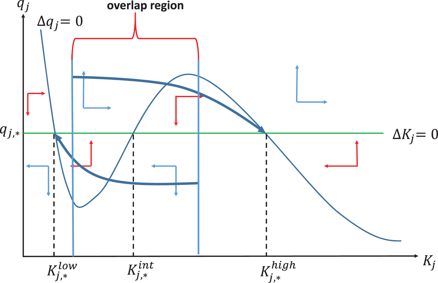
The emergence of multiple steady states hinges on the endogeneity of markups. Since m j = m j(K j), with  $m_{j}^{\prime }(K_{j})<0$, the marginal product of capital is not necessarily declining in K j (see Lemma 2). Thus, q j,* as defined by (32) may intersect (30) more than once in the {K j;q j}-plane, which gives rise to multiple steady states. From equation (26) and equation (30), we observe that
 $ q_{j}\gtrless q_{j,\ast }$ implies
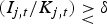 $(I_{j,t}/K_{j,t})\gtrless \delta $, such that in light of equation (24),
 $\Delta {K}_{j,t+1}\gtrless 0$. This situation is reflected by the horizontal vector arrows in figure 2. Above (below) the Δq j = 0-locus determined by equation (31), the sum of the marginal product of capital and marginal installation cost, ∂Y j,t+1/∂K j,t+1 + θη(I j/K j)1+η is, for a given q j, below (above) the level that would assure Δq j = 0. Thus for the region above the Δq j = 0 -locus, it follows that Δq j,t+1 > 0, while below we have Δq j,t+1 < 0.
Phase diagram with overlap region in the {K j, q j}-plane.
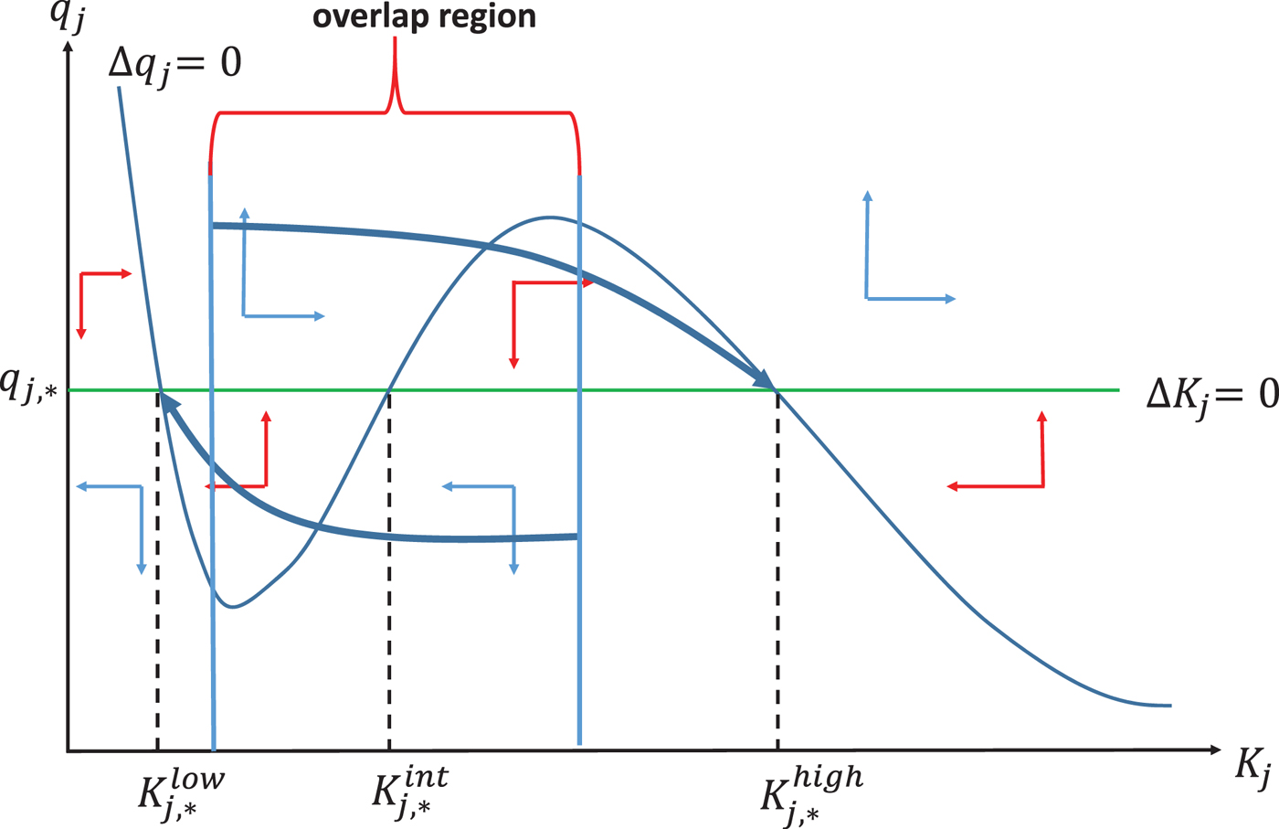
In figure 2, this situation is characterized by the vertical arrows. We therefore conclude that the case of three steady states in the figure is characterized by two exterior saddle-point stable steady states and one interior unstable steady state. In the dirty regime, the steady state with the highest capital stock implies the highest value of net output and consumption, given any level of initial wealth. However, as utility is negatively affected by pollution, highest output does not imply highest welfare; it depends on the shape of the utility function, specifically on the parameter ε.
Depending on the characteristics of the interior unstable steady state, the evolution of the economy may be subject to global indeterminacy. Thus, the trajectories leading to either the superior or the inferior steady state overlap such that expectations determine the equilibrium selection process. Outside the region of the overlap, initial conditions (history) determine whether the inferior or the superior equilibrium is reached. Energy taxes and the state of the economy, expressed by installed capital equipment, then determine whether history or expectations shape the transition to the inferior or superior equilibrium. The reason is that energy taxes affect factor productivity and thus the shape as well as the position of the Δq j = 0-locus. In our framework, q j relates to the net present value of one additional unit of capital.Footnote 10 This implies that the selection of the superior (inferior) transition path must be associated with favorable (unfavorable) fundamentals in an admissible fashion. An entrepreneur has optimistic expectations if she expects that everybody else has optimistic expectations regarding the net-present value of additional capital equipment. This is the common feature of self-fulfilling prophecy equilibria. In an extreme case, energy policy determines even the number of equilibria: if factor productivity ( $\tilde {A}_{d,t}$) is via high (low) energy taxes reduced (increased) drastically, only the inferior (superior) equilibrium can survive.
Conceptually, the existence of an overlap region requires that the interior unstable steady state be characterized by complex conjugate eigenvalues which assures that the topology of the phase diagram allows for a transition from the left (right) of the interior steady state to the superior (inferior) steady state. Below, we establish that the emergence of an overlap region and its size is affected by the tax level τ. Environmental preferences determining τ affect thus the relevance of history versus expectations for the equilibrium selection process. In the following proposition, we summarize how both, the location of the Δq = 0-locus as well as the role of expectations, depend on the total factor productivity of technology j ( $\tilde {A}_j$). Note that
 $\tilde {A}_{d,t}$ is then affected by the strength of green preferences (ε) which determine the energy tax (τ).
Proposition 3
(i) An increase (decline) in total factor productivity
$\tilde {A}_{j}$ moves the Δq j = 0-locus in the {K j;q j}-plane upwards, such that for a given set of parameters, only the inferior (superior) steady state survives if $\tilde {A}_j<\tilde {A}_{j,\min }$ ($\tilde {A}_j>\tilde {A}_{j,\max }$). In both cases, the dynamics of the economy is driven by initial conditions. The model exhibits three steady states if $\tilde {A}_{j} \in \lbrack \tilde {A}_{j,\min },\tilde {A}_{j,\max }]$. The interior steady state exhibits real eigenvalues if $\tilde {A}_{j}\leq \tilde {A}_{j,crit}$ and complex conjugate eigenvalues if $\tilde {A}_{j}>\tilde {A}_{j,crit}$.(ii) If j=d, the Δq j = 0-locus moves downwards during the transition to the steady state since ∂τt/∂K d,t > 0 and
${\partial \tilde {A}_{d,t}}/{\partial \tau _t}<0$.(iii) Higher ecological preferences induce higher energy taxes and a more pronounced reduction of
$\tilde {A}_{d,t}$.





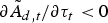

In light of the above proposition, the existence of three steady states requires that the total factor productivity (TFP) lie within the interval 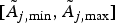 $\lbrack \tilde {A}_{j,\min },\tilde {A}_{j,\max }]$.Footnote 11 In the dirty regime, the total TFP is declining if the energy tax is increasing during the transition to the steady state. This implies that even though the model is initially characterized by the existence of three conditional steady states, only the inferior steady state may survive in the long run. The risk of the superior steady state vanishing increases in the magnitude of environmental preferences (ε) which increase energy taxes and induce thereby a more pronounced reduction in the TFP. If the TFP is above
 $\tilde {A}_{j,crit}$ and within
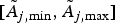 $\lbrack \tilde {A}_{j,\min },\tilde {A}_{j,\max }]$, the interior steady state is an unstable spiral and the dynamic system allows for the existence of an overlap region, such that expectations matter. At this stage, we can already conclude that high environmental preferences reduce the likelihood of the emergence of an overlap region in the dirty regime through increasing taxes and thereby potentially reduce the role of expectations compared to history.
6. Numerical experiments
The overlap region and its response to economic policies can only be detected numerically. For that reason we underpin the economic reasoning of our model with numerical experiments. With a variable energy tax,  $\tilde {A}_{d,t}$ is time-varying until the steady state is reached and thus the position of the Δq d = 0-locus as well. In order to isolate the effect of τt on the size of the overlap regions, we illustrate the overlap region for an initial value of the energy tax which is zero in our case and its steady-state value in the superior steady state, which is
 $\tau _*^{high}=0.5462$. We then present the dynamics of the energy tax (τ),
 $\tilde {A}_d$, and environmental quality (Q) for different degrees of environmental preferences (ε). Finally, we discuss the emergence of a regime switch to the green technology with different degrees of environmental preferences.
We set α = 0.3 and β = 0.18 such that the income share of energy is slightly above 0.1. The length of one period is around 30–35 years. A depreciation rate of 4 per cent per annum implies δ = 0.3. Business cycle literature suggests a discount factor of 0.99 per quarter for future consumption, such that ρ = 0.99120. As regards the investment cost function, we assume standard values, i.e., η = 1, which implies a quadratic cost function. The remaining values are set as follows: γ = 0.1, B d = 1, ψ = 0.0003, ε = 0.75;1,  ${\bar Q}=0.95$ and κ = 351. m(K) = σ(K)/σ(K) − 1, with
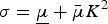 $\sigma = \underline \mu + \bar \mu K^2$, where
 $\underline \mu =1.0251$ and
 $\bar \mu =1.25$. Ω = 0.25 which amounts to 1/8 of the steady-state income level of one working cohort. We shall emphasize that despite implementing a reasonable model calibration, our goal is to characterize transitional dynamics qualitatively rather than quantitatively.
To start, we consider an economy that applies the dirty technology and imposes an energy tax of τ = 0. Moreover, 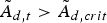 $\tilde {A}_{d,t} > \tilde {A}_{d,crit}$ such that the interior steady state exhibits two complex conjugate eigenvalues. In this case, there exists a region characterized by a range of the state variable (K d) around the interior unstable equilibrium (
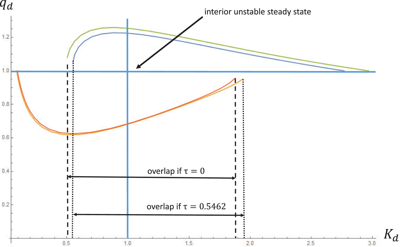
 $K_{d,*}^{int}$) in which the equilibrium trajectories to the exterior steady states overlap. Within this overlap region, the superior (inferior) steady state can be reached from the left (right) hand side of the interior steady state. Thus, knowledge about the initial state of the economy is insufficient for the selection of the equilibrium trajectory.Footnote 12 The transition to the superior (inferior) steady state is characterized by an associated q t,d above (below) its long-run value (q d,*). Since q j reflects the present value of an additional unit of physical capital installed in the representative firm net of capital adjustment costs,
 $q_{d,t} \gtrless q_{d,*}$ implies thus that
 $I_{d,t} \gtrless I_{d,*}$. The long-run value q d,* is just sufficient to sustain the steady-state capital stock in the sense that depreciated capital is replaced by investments (
 $I_{d,*}^s=\delta K_{d,*}^s$, s = low, int, high).
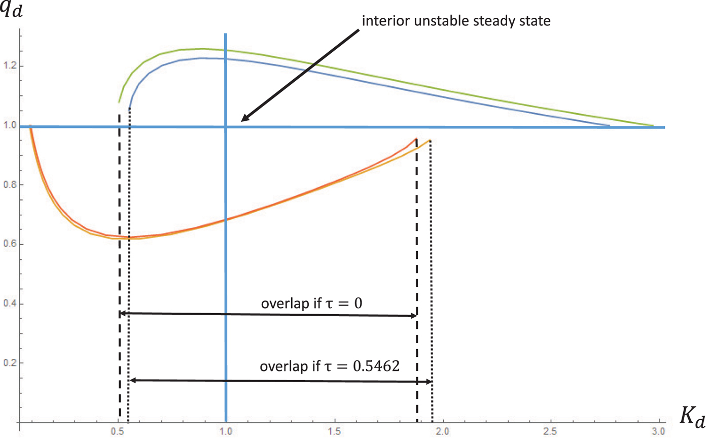
Figure 3 depicts the equilibrium trajectories in the {K d, q d}-plane to the exterior steady states. Moreover, it illustrates the effect of an increasing energy tax during the transition from τ0 = 0 to  $\tau _*=0.54624$ which corresponds to the steady-state level of the superior steady state in the numerical experiment below. Note that in figure 3 the interior steady state has been normalized to one. Since
 ${\partial \tilde {A}_d}/{\partial \tau }<0$, the levels of the exterior steady states are reduced. The change in the total factor productivity alters the size of the overlap region, indicated by the dashed compared to the dotted area. Apparently, the overlap region shrunk to the left of the interior steady state and increased to the right of it. As a consequence, the potentially positive influence of expectations for rather unfavorable initial conditions (K d,0) is reduced. At the same time, the overlap has grown in the area for comparatively favorable initial conditions, thus in the region where negative expectations can induce a transition to the inferior steady state despite the fact that the economy starts with favorable conditions. Hence, an energy tax reduces the likelihood of reaching the superior long-run equilibrium under unfavorable initial conditions but optimistic expectations. In fact, an energy tax increases the risk that the economy converges to the inferior steady state under comparatively favorable initial conditions but pessimistic expectations.
Equilibrium trajectories to the superior/inferior steady state for different energy taxes (τ = 0 and τ = 0.5462). The interior unstable equilibrium has been normalized to 1.
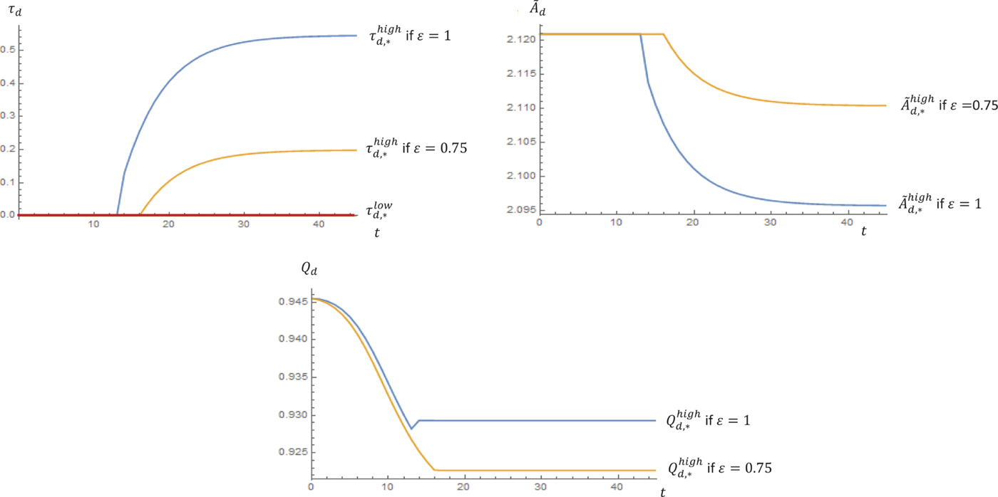
We now illustrate the transition of the energy tax from zero to its steady-state value which may be 0 or positive depending on whether the economy is converging to the inferior or the superior steady state. The transition paths for the energy tax (τ),  $\tilde {A}_d$ and environmental quality (Q) for different degrees of environmental preferences (ε) are depicted in in figure 4. The inferior and the interior steady states are characterized by
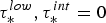 $\tau _*^{low},\tau _*^{int}=0$. Since the endogenous energy tax is an increasing function in K d, the tax must become positive somewhere to the right of the interior steady state. While the transition to the inferior steady state is characterized by τt = 0, the representative household supports an energy tax at later stages of the transition to the superior steady state. The increase in the energy tax reduces
 $\tilde {A}_{d,t}$ towards its steady-state level. Therefore, the size of the overlap is time varying during the transition to the steady state as well.
Transition paths for the energy tax (τ),  $\tilde {A}_d$ and environmental quality (Q d) for different degrees of environmental preferences (ε).
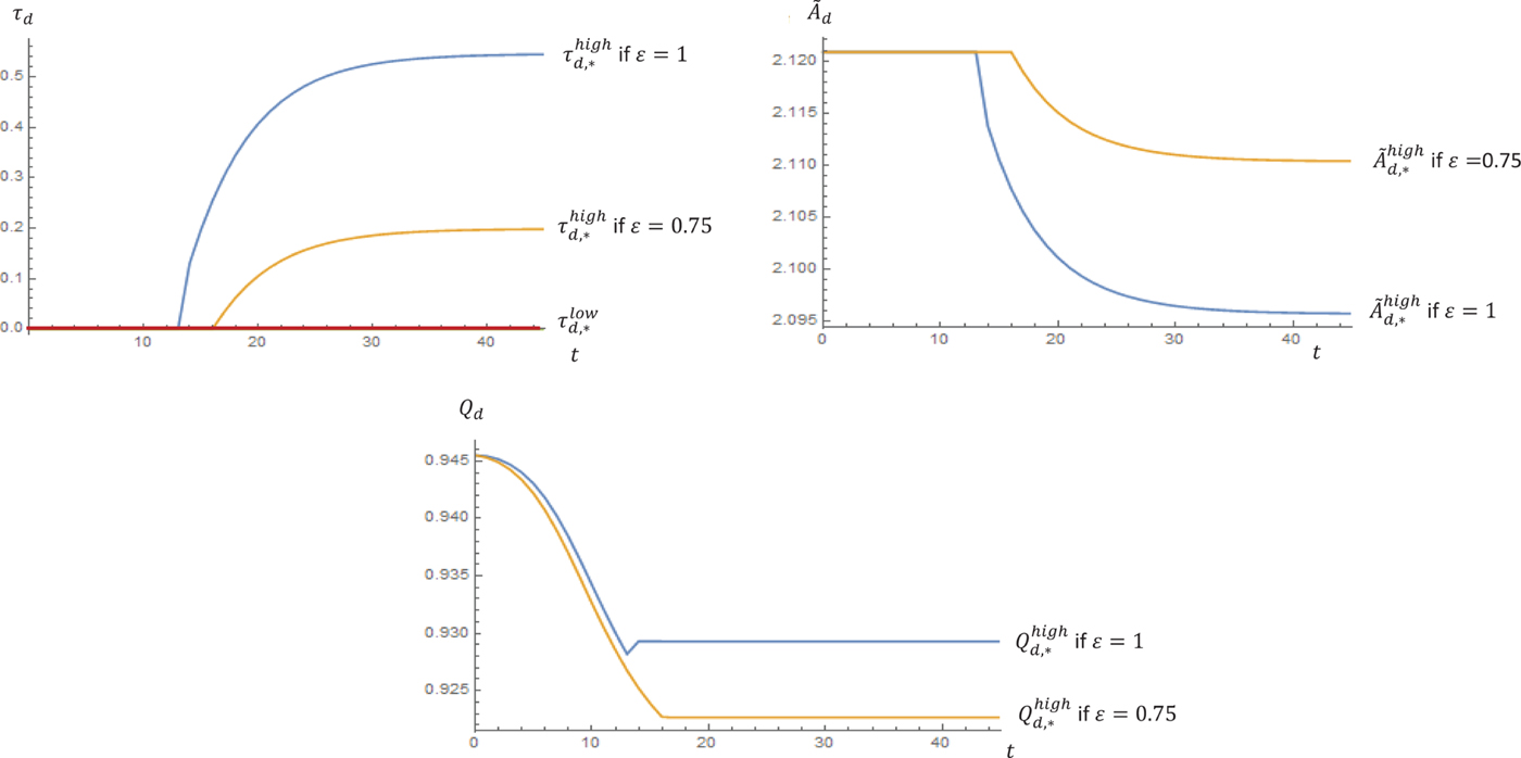
The initial size corresponds to the τ = 0 case in figure 3 and approaches the τ = 0.5462-case. Thus, the importance of expectations is changing during the transition. Initially, for  $K_{d,0}<K_{d,*}^{int}$, the prospects of selecting the trajectory leading to the superior steady state are more favorable during earlier stages of the transition. As the energy tax is increasing at later stages, the overlap is declining to the left of the interior steady state but increasing to the right of it. Thus, the risk of selecting the trajectory leading to the inferior steady state, if expectations are pessimistic, is increasing. Higher preferences for environmental quality (ε) increase the energy tax in the long run. As societies with higher environmental concerns impose a higher energy tax, the total factor productivity is declining during the transition to the steady state to a lower level which is compensated from the welfare perspective by a higher level of environmental quality (Q). The associated reduction in the overlap region leaves less room for favorable economic development if expectations are optimistic and the economy is located to the left of the interior unstable steady state. On the other hand, the importance of expectations is increasing to the right of the interior steady state. An economy located in this region could reach the superior equilibrium if only history mattered. It faces, however, now the risk that pessimistic expectations induce the selection of the trajectory to the inferior equilibrium. Nevertheless, our empirical motivation in the introduction suggests that societies with higher ecological preferences tend to be more optimistic with respect to future economic development. Whether or not this is the case is indeed an empirical question which needs to be more substantiated. We come back to this aspect in the subsequent section. If, hypothetically, an economy characterized by a relatively high ε tends to be more optimistic with respect to future economic development, the risk that this economy will coordinate itself towards the inferior steady state may not be relevant. On the other hand, the role of optimistic expectations to the left of the interior steady state is reduced since the overlap region has shrunk in that area.
In that sense, we can conclude at least from a theoretical point of view that higher environmental concerns increase the role of expectations under favorable initial conditions, while the overlap region is reduced to the left of the interior equilibrium such that the equilibrium selection process becomes more history-dependent there. Hence, optimistic expectations are of little help in this region. If societies with higher ecological concerns tend to implement higher energy taxes, the overlap region where optimistic expectations are supportive for the selection of the superior equilibrium is reduced and increased in a region where optimistic expectation may just prevent these societies from selecting the inferior transition path. Again, whether or not this risk exists is an empirical question which will be analysed in the subsequent section.
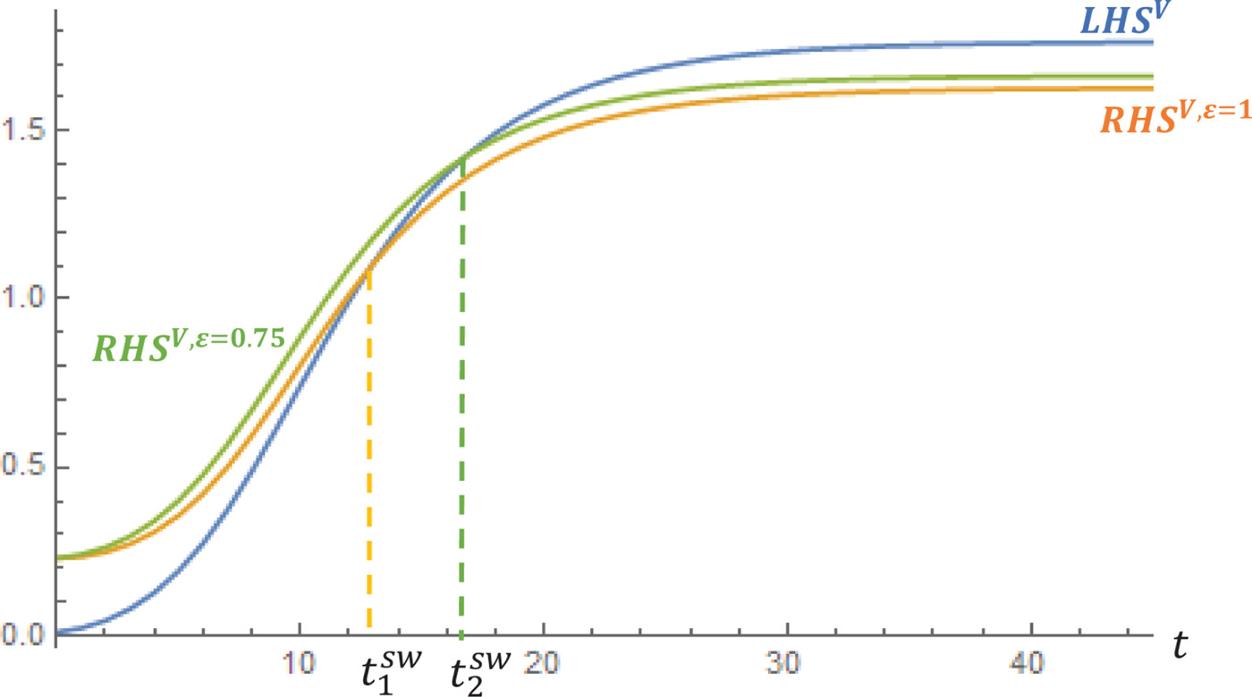
Consider now the scenario of an endogenous regime switch, i.e., the representative household compares the resulting lifetime utility levels in regime d and regime c supporting a regime switch, if V c,t ≥ V d,t, such that in light of Proposition 2,
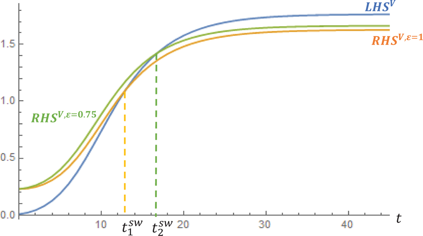
 $$\underbrace{w_{c,t} - \Omega}_{LHS^V} \geq \underbrace{\displaystyle{w_{d,t} \over ( {Q^{\max}}/{Q_{t+1}})^{{\varepsilon}/{(1+\rho)}}}}_{RHS^V}.$$
In regime c environmental quality is disconnected from the production process. Thus, environmental quality is at its maximum level (Q max). Moreover  $\tilde {A}_c$ is constant and so is the size of the overlap region.
In light of the previous discussion the size of the overlap in regime c depends on  $\tilde {A}_c$. If the clean technology is sufficiently productive, the overlap of the green technology may be larger to the left of the interior steady state compared to regime d. Then, the regime switch increases the role of expectations compared to history in this region and reduces the role of expectations to the right of the interior unstable steady state. If households are more optimistic with respect to future economic development, the regime switch increases the likelihood of the superior equilibrium being selected.
This mechanism is reinforced by the magnitude of environmental preferences which induce in regime d a faster decline in  $\tilde {A}_d$ relative to
 $\tilde {A}_c$.
In figure 5, we depict the evolution of the left-hand side and the right-hand side of (33) for different degrees of environmental preferences (ε). Higher environmental preferences attach a higher weight to environmental quality, such that a higher ε shifts the RHS-curve downwards. Consequently, societies with a higher ε switch earlier compared to societies with a smaller ε.
Regime switch to the clean regime for ε = 1 and ε = 0.75. RHS V = w d,t/(Q max/Q t+1)ε/(1+ρ) and LHS V = w t,c − Ω.
So far we have assumed that the state collects energy taxes, but we have been silent about the use of the tax revenues. Implicitly, we presumed that the state spends the tax revenues unproductively. One could object that the conflict between ecological preferences and  $\tilde {A}_d$ is biased due to the absence of measures reducing the conflict between the polluting technology and the environment. We abstract from the existence of an abatement technology since it is analytically less tractable and we do not gain more information in view of the research question of this paper. In the online mathematical appendix, we generalize our arguments with respect to the existence of an abatement technology and show that the presence of tax-financed abatement measures does not constitute a conflict regarding our arguments. If an abatement technology is active, the preferred tax rate is still increasing in ε but also in the effectiveness of abatement measures, since the marginal benefit of taxation (higher environmental quality) is increasing by more than the marginal cost.Footnote 13
7. Robustness
Our small-open-economy assumption allows us to analyse the incentives for ambitious environmental policies in countries with rather minor impacts on global pollution levels. Following the logic of the Paris Agreement, all countries commit to reducing their national emissions. Despite most countries' very low share of total global emissions, they all handed in a pledge with their nationally determined contribution. One important, but often neglected, element is that most policies aiming to mitigate climate change profit from local side benefits, such as a reduction in polluting particles and noise (Hamilton et al. (Reference Hamilton, Brahmbhatt and Liu2017)). Hence, our environmental quality should rather be interpreted as domestic quality that can be improved with domestic measures. In the model we thus abstracted from a global pollutant affecting domestic environmental quality. For the sake of clarity we also assumed a regeneration capacity of the environment from one period to another of 100 per cent. In this section we extend the analysis to: (1) incomplete regeneration of the environment (0 < δQ < 1), and (2) the impact of global pollutants on the domestic economy, resembling a global challenge such as climate change. While the main reasoning of our paper remains robust with respect to these changes, we obtain interesting results regarding the timing of a switch from the polluting to the green energy regime and the importance of expectations in the polluting regime.
(1) Incomplete regeneration of the environment (0 < δQ < 1): For 0 < δQ < 1, the dynamics of the economy is governed by a three-dimensional system of difference equations as described by (17), (24) and (25). Conceptually, δQ < 1 affects the level of the preferred energy tax, therefore total factor productivity in the polluting regime ( $\tilde {A}_{d,t}$) and hence the timing of the regime switch to the green regime. The immediate impact of a reduced regeneration capacity is a reduction of environmental quality implying an increase in the preferred energy tax (∂τt/∂δQ < 0). Hence, total factor productivity
 $\tilde {A}_{d,t}$ shrinks. With this information at hand, we are prepared to derive the impact of δQ on the regime switch. Again a regime switch occurs if V c,t ≥ V d,t, where the fundamental difference compared to (33) arises from the fact that environmental quality does not jump to its maximum level after the regime switch but to
 $Q_{c,t+1} = \delta _Q {\bar Q} + (1-\delta _Q) Q_{c,t}$, such that (33) transforms to
 $$\underbrace{w_{c,t} - \Omega}_{LHS^V} \geq \underbrace{\displaystyle{w_{d,t} \over ( {\delta_Q {\bar Q} + (1-\delta_Q) Q_{c,t}}/{\delta_Q {\bar Q} + (1-\delta_Q) Q_{d,t} - P_t})^{{\varepsilon}/{(1+\rho)}}}}_{RHS^V}.$$
From the discussion above, it follows that δQ reduces through higher energy taxes w d,t. Moreover, for any given Q t and P t, the denominator of RHS V increases such that a lower regeneration rate of the environment makes an earlier regime switch more likely.Footnote 14 This reasoning is depicted in figure A1 in the online mathematical appendix.
(2) Global pollutants: Due to the small open economy assumption, the stock and the evolution of global pollutants is exogenous to the domestic economy. Domestic environmental quality is affected by the stock of domestic and global pollutants, i.e.,  $Q_{t+1} = {\bar Q} - \kappa _g S_{t+1}^{global} - S_{t+1}$, such that
 $$Q_{t+1} = \delta_Q {\bar Q}_t + (1-\delta_Q) Q_t -P_t,$$
with  ${\bar Q}_t = {\bar Q} - {\kappa _g [S_{t+1}^{global}+S_t^{global}]}/{\delta _Q} - \kappa _g S_t^{global}$, where κg ≥ 0 represents the adverse impact of global pollutants on domestic environmental quality.
Hence, increasing threats through climate change are captured by a decline in  ${\bar Q}_t$ and the mitigation of climate change, for example through the Paris Agreement, would be captured by an increase or a slower decline to a higher steady-state value of
 ${\bar Q}_t$. Higher climate risks increase the energy tax (∂τt/∂κg > 0), reduce w d,t and increase everything else equal the denominator of RHS V,Footnote 15 such that accelerated climate change makes an earlier regime switch to the green energy regime more likely in the domestic economy. Finally, the associated increase in energy taxes through a higher exposure to global pollutants reduces the role of expectations in the polluting regime (see figure A2 in the online mathematical appendix).
8. Empirical analysis
Our model proposes an interplay between ecological preferences and expectations about economic development. To derive implications for the real-life setting, we analyse empirically whether there is a relationship between green preferences and expectations.
As introduced in section 1, beliefs about the future play an important role in economic development by influencing current decision making and thereby work as self-fulfilling prophecies. The successful transition to a clean energy regime may thus depend on people's willingness to support environmental measures but also on their economic expectations. The factors driving positive or negative expectations are debated. Furnham (Reference Furnham1997) suggests that personal traits such as age, income, faith and political attitudes can explain partly whether someone is more of an optimist or a pessimist. It is also assumed that people include external information such as media information or historic economic development in addition to emotional beliefs (e.g., Bafumi, Reference Bafumi2011). A new strand of literature emphasises the current power of the preferred political party: people tend to be more optimistic about the economy if they are ideologically aligned with the party in power (Stokes, Reference Stokes2017). Based on the Eurobarometer analysis shown in figure 1, we hypothesise that there is also a relationship between environmental attitudes and expectations about economic development. If people value environmental protection, they may be both; that is, willing to implement stricter policies in favor of the environment and more optimistic that the new policies define a good framework for economic prosperity. Such optimism may have gained momentum with scholars forecasting the creation of new jobs linked to environmentally-friendly industries (Fankhauser et al., Reference Fankhauser, Sehilleier and Stern2008). Others argue that environmental protection should be implemented soon, since it will become more expensive, the longer we wait (Stern, Reference Stern2006). Following that argument, environmental measures depict a necessity for future economic growth and thereby drive optimism. In our literature research we could not find any data analysis that has addressed this question. One important reason may be that there is little data available. Most of the opinion surveys and thus the related analyses combine the two opinions in a contradicting question. Namely, respondents have to choose which of the two they consider more important, either environmental protection or economic performance. This way data analysts are unable to find a potentially positive relationship between the two attitudes.
8.1. Data
We use data from the Selects survey 2015, which is part of a long-term election study by FORS Switzerland (Selects, 2017). The aim of this survey is to analyse and forecast political participation and the decision-making process of the Swiss population. The opinion poll 2015 contains four different parts: a one-time survey after the elections, a panel survey with three waves before and one wave after the elections, a media analysis and a candidates survey. For our main analysis, we make use of the first part of the panel survey (wave 1) where participants are asked questions regarding: a) their opinion about the necessity of stricter measures for the environment, and b) their expectations about the development of the economy in Switzerland. Both questions are asked in a similar format. Respondents had to choose on a 5-point Likert scale ranging from ‘Strongly in favor’ to ‘Strongly against’ with respect to the question: ‘Are you in favor of more environmental protection in Switzerland?’ and from ‘Improve significantly’ to ‘Worsen significantly’ for the question ‘How do you expect the economic situation in Switzerland to be like in one year from now’. A random, but representative sample with participants from all over Switzerland was interviewed online. In total 11,047 people participated, out of which 5,618 were men and 5,429 women. Due to missing data points, we had to exclude 156 participants for the basic estimation and a further 384 participants for the estimations with more control variables.
As a starting point for the theoretical reasoning (see figure 1), we analysed data from the Eurobarometer 2016 dataset. The standard Eurobarometer 85 census was carried out in May 2016 in 33 countries. It examines Europeans' attitudes on the domestic and European political situation, their main concerns and their perception of domestic and EU institutions (Eurobarometer, 2016). In the survey 2016, interviewees are asked about both, what they think are the most important issues affecting their country (max 2 issues, free text) and their opinion on the future economic system (choice of the options better, worse or equal). With a basic multi-stage random design in each country, a total of 32,987 participants were interviewed.
8.2. Empirical strategy
We use a multinomial ordinal logit regression model to test the effect of the attitude regarding environmental protection on the likelihood of choosing each option of the question about economic expectations. We regress the environmental opinion variable on the expectations variable, controlling for two groups of variables: socio-economic variables and political opinion variables. In the group of socioeconomic variables we control for household income, highest education degree, sex, age and canton of residence. In the group of political opinion variables we control for the respondent's party choice and which problem area is considered to be the most important. Following the findings in the literature about the importance of the party in power to shape expectations, we also control for the expectations about which party is going to win (and would thus gain more or less power in the political decision-making process). For that, we create a binary dummy variable based on two questions in the survey. We combine the answer about the party choice of the respondent with the expectations about whether this same party is going to win or lose in the coming elections. For respondents who think that their party is very likely to win, we assign a value of 1, for the others a value of 0.
8.3. Results
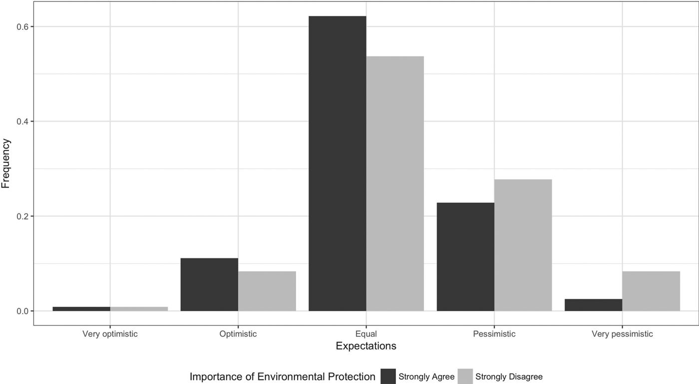
Our analysis indicates that expectations about economic development differ for people with different environmental attitudes. While the distribution of the answer patterns is alike, interviewees who strongly disagree with having stricter environmental protection seem to be less optimistic with respect to economic development (see figure 6). Put another way, people who indicate that they are in favor of stricter environmental measures tend to have more optimistic expectations about the future of the economy.
Relationship between attitudes on environmental protection and economic expectations. Data: Selects, 2015.

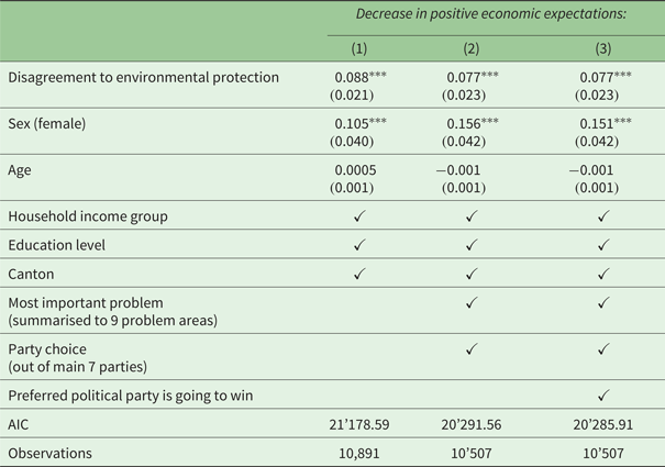
In table 1 the reader can see that the coefficient measuring the attitude on environmental protection is highly significant. In column (1) we control for socioeconomic variables only. In column (2) we include the answers on the party choice and the most important problem area to be solved. In column (3) we also control for whether the respondent is confident that the respondent's elected party is very likely to win in the elections. The interpretation is as following: the log odds for being less optimistic increase significantly for people who disagree with stricter environmental protection. Thus, for respondents who do not strongly agree with stricter environmental measurements (which is the reference scenario), the ordered log-odds that they also respond more pessimistically regarding economic development increase by 0.077. The data analysis also indicates that female respondents are more likely to be pessimistic about economic development compared to male respondents, whereas we do not find a significant impact of age.
Multinomial ordinal logit regression

Note: *p<0.1; **p<0.05; ***p<0.01
The coefficient indicating that a participant disagrees with more environmental protection (compared to the baseline of strong agreement) significantly increases the log odds of choosing a more pessimistic answer option regarding expectations about economic development.
Data: Selects, 2015.
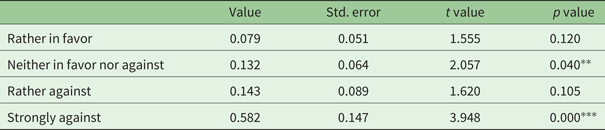
In table 2 we separately analysed each answer option with the baseline scenario. One can see that the coefficient is highly significant for the respondents who are strongly against environmental measures compared to the ones who are strongly in favor. The interpretation is that for a male participant who is strongly against stricter environmental measures, the ordered log-odds of being more pessimistic about economic development increases by 0.582 compared to the baseline scenario (someone who is strongly in favor of more strict environmental measures), ceteris paribus all other variables. The coefficient is positive and increases for all answers compared to the baseline (from rather in favor to strongly against). However the coefficients are only significant for the participants who are neither in favor nor against and the ones who are strongly against.
Separate analysis for environmental opinion variable on expectations about economic development

The log odds for choosing a more pessimistic answer option (compared to the baseline Improve significantly) is highly significant for people who strongly disagree with environmental protection compared to the ones who strongly support it.
Data: Selects, 2015.
8.4. Robustness checks
As a robustness test we create a dichotomous dummy variable for participants who are either in favor of or against environmental measures. Including this variable instead of the 5 scale answer variable, the results remain significant on the 5 per cent level.Footnote 16
In order to exclude multicollinearity between the variables, we apply a variance inflation factor (VIF) test. The variable of interest has a VIF test coefficient of 1.396 only and we can thus be confident about excluding multicollinearity issues for our variable.Footnote 17
A standard issue with such questionnaires is that participants differ in their general response behaviour due to personal traits. It is, for example, possible that some people are generally more worried than others. In wave 3 of the panel survey, respondents are asked to rate themselves on a 10-point scale with regard to whether: (1) they consider themselves as a person that is often worried, and (2) if they are usually relaxed in stressful situations. We run the same regression including those two variables. The coefficient of interest remains significant at the 1 per cent level.Footnote 18
8.5. Discussion
Our empirical analysis sheds light on the relationship between environmental attitudes and economic expectations. The results of the data analysis show that interviewees who are in favor of stricter environmental protection also tend to be more optimistic with respect to economic expectations. This supports our hypothesis that is based on the initial analysis of the Eurobarometer 2016 dataset. Moreover it questions common wisdom that people are in favor either of green policies or economic development.
The findings can be used for the discussion of the dynamics along the saddle path and thus projections about the steady state in our model. The observation of a relationship between pro-environmental attitudes and optimistic expectations (and vice versa) implies that: (a) if societies with higher ecological concerns tend to implement higher energy taxes, the overlap region where optimistic expectations are supportive for the selection of the superior equilibrium is reduced and increased in a region where pessimistic expectations are influential. Nevertheless, their high degree of optimism may prevent these economies from converging to the inferior steady state. (b) If societies with higher ecological concerns assume an earlier regime switch, their high degree of optimism likely drives a transition to the superior steady state.
The survey is created such that the Swiss population is well represented. However, the reader should be aware of some common, immanent limitations linked to such samples, in particular self-selection biases, dishonest response behaviour and a certain under- or over-representation of subgroups of the population. One particular limitation is that people's opinions may differ greatly when it comes to the acceptance of concrete policy instruments (e.g., Vimentis, 2018). Our dataset describes people's general attitudes with respect to more environmental protection but does not specifically ask about a tax as assumed in the model. However, we think that we mitigated this potential, rather uncircumventable conflict by our modeling strategy, since we considered a rather stylized and general tax instrument.
Also, note that the largest share of the survey participants are neither optimists nor pessimists. However, the overall number of pessimists is higher than the number of optimists. Hence, even with a more environmentally-friendly population, the risk of taking the saddle path to the inferior steady state is decreased but still substantial. From a policy-making perspective, this finding calls for additional analysis and research as to whether and if so how it is possible to shape expectations to become more optimistic.
9. Conclusions
In an overlapping generations model with multiple steady states, we analysed the impact of endogenous environmental policies on the relevance of history and expectations for the equilibrium selection process. We considered two production regimes: a polluting regime with an endogenous energy tax and a clean regime subject to switching costs. In the polluting regime, an increasing energy tax raises – under pessimistic expectations – the risk of the economy transitioning to the inferior equilibrium. The reason for this dilemma is rooted in the adverse effect of energy taxes on the total factor productivity in the polluting regime. The reduction in total factor productivity reduces incomes in the short and long run and it reduces the region of state variables in which positive expectations matter for the equilibrium selection process, but increases the region where negative expectations matter (overlap region).
We have shown that a switch from dirty to clean production depends on the productivity of both technologies, on the level of pollution and on the preferences of the households for environmental quality. With an endogenous energy tax, the size of the overlap is time-varying. An early increase in the tax (due to strong environmental preferences) decreases the factor productivity gap between the two technologies. A switch to clean production occurs earlier and decreases the trade-off between environmental preferences and total factor productivity. Thus, higher preferences for the protection of the environment imply an earlier switch to the clean energy regime. In this regime, the conflict between production and environmental preferences is not only resolved, but the prospects of selecting the superior equilibrium have increased, since this regime gives more space to expectations compared to history, given that the productivity of the clean technology is sufficiently high.
In an empirical data analysis from a large election survey in Switzerland, we find that people with strong environmental preferences are more likely to also have more optimistic expectations about economic development. The positive relationship between environmental preferences and economic optimism scrutinises the common wisdom that people are either in favor of the environment or economic development.
The findings have important implications for the steady-state analysis of our model: in a policy scenario without switching possibilities, the likelihood of reaching the inferior stable steady state is low, due to the generally optimistic expectations (despite the fact that the area where positive expectations matter becomes smaller). Second, for societies with strong environmental preferences, the switch to a clean production happens faster, because they will support higher energy taxes which makes an early switch more attractive. As a result of their optimistic expectations, the likelihood of reaching the superior steady state increases.
Supplementary material
The supplementary material for this article can be found at https://doi.org/10.1017/S1355770X19000135.
Acknowledgments
We wish to thank Lucas Bretschger, Chiara Colesanti, Elise Grieg, and participants at IWECCS 2018 (Bologna), SURED 2018 (Ascona), WCERE 2018 (Gothenburg) as well as seminar participants at the University of Bath, ETH Zurich, and the University of Goettingen for instructive suggestions and constructive comments. Funding from the Swiss Federal Institute of Energy is gratefully acknowledged. Moreover, we wish to thank two anonymous referees for their valuable comments and suggestions!