I. INTRODUCTION
Elastic, elastic–plastic, and fully plastic regimes were observed for conical indentation.Reference Love1–Reference Mata and Alcala4 The deformation process produced during conical indentation is well described by LoveReference Love1 when the regime is elastic. When plasticity occurs, it is more complex to describe indentation responses because the material of the sample exhibits multiaxial stress conditions with high gradients and large elastic–plastic strains in the indentation region. Strong nonlinearities are induced by the unilateral contact and the involved large displacements. A pile-up can be also developed during the indentation test. Because of the complex nature of the strain field produced by an indentation, the first analytical solutions have been limited to rigid-ideally plastic or elastic materials. For the former, TaborReference Tabor3 has shown that the mean indentation pressure H is related to the material flow stress Y by

where C f is a constant, called “constraint factor,” depending upon the geometry of the indenter with a value near 3.
Slip line pattern also leads to Eq. (1) for frictionless cone penetrating a flat surface if the semi-apex angle of the cone is large.Reference Johnson2 It was shown that this simple hardness theory is deficient for highly elastic materials.Reference Marsh5 Attempts were made to correlate indentation pressure in elastic–plastic materials using the theoretical analysis of the expansion of a cylindrical or spherical cavity by an internal pressure.Reference Marsh5–Reference Mata, Casals and Alcala7 The most famous of these was by Johnson.Reference Johnson8 He considered the indenter to be encased in a hemispherical core of radius a, which replaces the cavity in Hill’s model.Reference Hill9 A hydrostatic uniform pressure is assumed to exist throughout the core, equal in magnitude to the mean indentation pressure. In the Johnson’s model,Reference Johnson8H is related not only to the yield stress (Y) but also to the Young’s modulus of the indented material (E) and the geometry of the indenter as well. The expanding cavity model (ECM) involves certain key assumptions such as a not purely hydrostatic stress in the material immediately below the indenter. This assumption gives better agreement with experimental data but introduces other inconsistencies. The basic difficulty is that the assumption of a true hydrostatic pressure in the core is not valid. Other shortcomings of this model have been pointed out in the literature, and some remedial measures have been suggested.Reference Studman, Moore and Jones10–Reference Feng, Qu, Huang and Nix12 Studman et al.Reference Studman, Moore and Jones10 pointed out a step-discontinuity in the stress field at the core–plastic zone interface. An improved result is obtained if it is assumed that the hemispherical core is a region in which the stresses are changing from purely hydrostatic to values satisfying the Von Mises yield criterion.Reference Studman, Moore and Jones10 This modification introduces also other inconsistencies. Another defect pertains to the nonvanishing normal traction outside the contact zone on the specimen surface, which is an outcome of applying Hill’s solutionReference Hill9 for a spherical cavity directly to the indentation problem. There have been two elegant treatments to account for the specimen surface. The first is Chiang’s revised expanding model.Reference Chiang, Marshall and Evans11 They calculated an auxiliary field generated by the exact negative tractions applied on the surface of a half-space, and then they could represent the free surface by summing the auxiliary field with the original solution. The second model to account for the surface effect is based on the Yoffe’s surface inclusion model.Reference Yoffe13 According to this model, Feng et al.Reference Feng, Qu, Huang and Nix12 proposed that the stress distribution outside the contact-induced plastic zone can be estimated by the superposition of a Hertzian field and an embedded center of dilatation (ECD) in a half-space, while the residual stress distribution can be estimated by the ECD field alone. Because of their complexity, these approaches have not been widely used in practice.
Notwithstanding these inherent assumptions and limitations, the ECM is still being used to interpret indentation data in ductile solids.Reference Fischer-Cripps14, Reference Kramer, Huang, Kriese, Robach, Nelson, Wright, Bahr and Gerberich15 The reason for the enduring popularity of this model is its simplicity and ability to predict with reasonable accuracy important experimental results such as the indentation stress versus strain curve, evolution of plastic zone size with load, and stress distribution beneath the indenter.Reference Johnson2, Reference Johnson8, Reference Fischer-Cripps14, Reference Kramer, Huang, Kriese, Robach, Nelson, Wright, Bahr and Gerberich15
The objective of this article is to provide a new ECM for describing conical indentation. We show that the Johnson’s ECMReference Johnson8 based on the conservation of volume during an increment of penetration can be replaced by an ECM based on the equality between the displaced volumes and the volume loss in the indented material. In a first step, it is assumed that the volume of material displaced by the indenter is equal to the volume loss, due to elastic deformation, in the core, plastic zone, and elastic zone. In a second step, we propose a new formulation of ECM for materials that exhibit pile-up or sink-in. It was shown that the Johnson’s ECM fits very well experiment data in the elastic–plastic regime, i.e., the transitional regime where H lies between 0.5Y and 3Y.Reference Johnson2, Reference Studman, Moore and Jones10, Reference Fischer-Cripps14 The purpose of this article is also to show that the results of ECM can be in agreement with numerical results in regimes, whose contact response is more plastically dominated, if pile-up or sink-in is taken into account in the model.
II. JOHNSON’S ECM
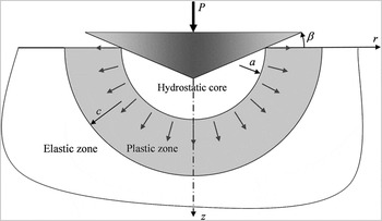
It is assumed that the elastic–plastic regime begins when the yield point is exceeded and occurs up to the fully plastic regime for which the elasticity is considered as negligible. In this regime, the plastic zone is contained by material which remains elastic. For the elastic–plastic regime, MarshReference Marsh5 and JohnsonReference Johnson8 suggested that the material in the indented zone can be viewed as being encased in an expanding hemispherical core. The proposed model is based on the compatibility between the volumetric expansion of the core and the volume of material displaced by the indenter. In this context, it was considered that (i) the hemispherical core is incompressible and subjected to an internal pressure, (ii) the radius of the core, a, is equal to the contact radius, and (iii) the hydrostatic stress within the core is equal to the radial stress at the core boundary (Fig. 1).
Schematic illustrating the Johnson’s expanding cavity model (ECM) for conical indentation.

Outside the core, it is assumed that the stresses and displacements have radial symmetry. The stresses in the plastic zone, a ≤ r ≤ c, are given by HillReference Hill9:

In the elastic zone, r ≥ c:

At the interface between core and the plastic zone, the hydrostatic stress in the core is just equal to the radial component of stress in the external zone, σr:

Based on the radial displacements within the plastic zone given by Hill,Reference Hill9 conservation of volume, and concept of geometrical similarity of the indentation, the ratio of the plastic zone size to the contact radius is

where β is the inclination of the face of the cone to the surface.
III. NEW FORMULATION OF THE ECM
A. Ratio of the plastic zone size to the contact radius
For the new formulation, it is assumed that the volume of material displaced by the indenter is equal to the volume loss, due to elastic deformation, in the core, plastic zone, and elastic zone:

where ∆V i is the volume of material displaced by the indenter, ∆V c, ∆V p, and ∆V e are the volume loss due to elastic deformation, respectively, in the core, plastic zone, and elastic zone.
For conical indenters, the volume of material displaced by the indenter is
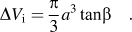
The volume loss in the elastic zone is

where ur=c is the radial displacement at the elastic–plastic interface.
The volume loss in the plastic zone is

where ur=a is the radial displacement at the core–plastic zone interface.
Using the Hill’s solution for ur=a in Eq. (9) leads to
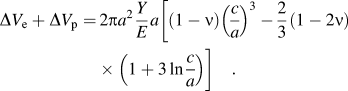
For the proposed formulation of ECM, constant hydrostatic pressure in the core and continuous stress field at the interface between core and plastic zone are assumed, i.e.,
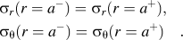
With these assumptions, the constant hydrostatic pressure in the core is equal to
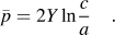
On contrary to the Johnson’s formulation, the stress in the core is not purely hydrostatic in our formulation. With the concept of geometric similarity of the indentation, i.e., c/a = constant,  is constant during indentation.
The advantage of the proposed formulation is that continuity in the Von Mises stress field exists at the interface between core and plastic zone on contrary to the classical formulation of the ECM.Reference Johnson8 The assumption of continuous stress field at the interface between core and plastic zone is incompatible with the assumption of hydrostatic core. In consequence, the mean indentation pressure cannot be determined starting from the hydrostatic pressure.
From Eq. (12), it follows that the volume loss in the core is

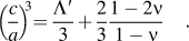
Substituting Eqs. (7), (10), and (13) into Eq. (6) then leads to

Notice that, for low cone angle, Eq. (14) is similar to the Johnson’s formulation [Eq. (5)].
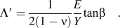
Hernot and PichotReference Hernot and Pichot16 show that the degree of deformation at the transition between the elastic–plastic regime and plastic regime depends on the normalized deformation Λ′. In the case of conical indentation, Λ′ is
It thus follows that
B. Indentation pressure
The equilibrium of the core leads to the indentation load:

where H is the indentation pressure.
The Johnson’s formulation,Reference Johnson8 with a condition of purely hydrostatic stress in all parts of the core, is similar to Eq. (17). It was shown that this equation is inadequate to fit indentation experiments.Reference Johnson2, Reference Studman, Moore and Jones10 Indeed, in Johnson’s article, his theoretical curve lies completely beneath the data points by a roughly constant amount up to pressures where fully plastic behavior ensues. For Johnson,Reference Johnson2 the problem is due to the fact that the stress in the material immediately below the indenter is not purely hydrostatic and thus the indentation pressure is not equal to the purely hydrostatic stress. Johnson modified his formulation to obtain a best estimate of the indentation pressure. In a similar way, Eq. (17) is modified to obtain better agreement between theoretical and experimental results:

Because of the proposed assumptions for the new ECM, it is not possible to keep the same arguments that the Johnson arguments to explain the modification added to Eq. (17).
For the authors, Eq. (17) gives bad agreement with the experimental data because the proposed assumptions only give an approximation to the real system. Equations (2) and (3) are obtained with the assumption that the indentation of an elastoplastic half-space is equivalent to a spherical cavity expanding in an infinite medium. However, the spherical symmetry around a cavity in an infinite medium does not match the symmetry around an indentation on a half-space involving a free surface. For example, σθ must be equal to zero on the free surface and it is not the case by using the Eq. (2).
IV. NEW FORMULATION OF ECM CONSIDERING PILE-UP AND SINK-IN
Johnson performed his study with the assumption that no piling-up or no sinking-in occurs during indentation. We propose, in this section, a new formulation of ECM for materials that exhibit pile-up or sink-in.
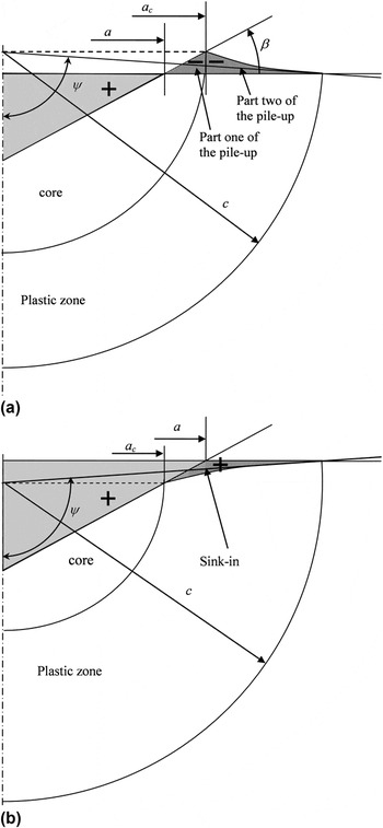
For materials that exhibit pile-up, it is assumed that the volume of material displaced by the indenter is equal to the pile-up volume and the volume loss, due to elastic deformation, in the core, plastic zone, and elastic zone [Fig. 2(a)].
Schematic illustrating elastic–plastic indentation as idealized by the ECM considering surface deformation. (a) pile-up and (b) sink-in.

For materials that exhibit sink-in, it is assumed that the volume of material displaced by the indenter and the sink-in volume are equal to the volume loss, due to elastic deformation, in the core, plastic zone, and elastic zone [Fig. 2(b)].
A. Materials that exhibit pile-up
The equality between the displaced volumes and the volume loss in the indented material is:

where ∆V pu is the volume of the pile-up.
The radius of the core is equal to a c and the volume of material displaced by the indenter is calculated starting from a [Eq. (7)]. The volume in the pile-up can thus be determined by geometrical conditions. The volume of the pile-up is calculated from:

where h is the penetration depth and h c is the contact height.
In this equation, C 1 quantifies the degree of pile-up and sink-in during the indentation test; C 1 > 1 indicates pile-up, whereas, C 1 < 1 accounts for sink-in.
The volume in the pile-up is divided into two parts. The first part corresponds to the volume of pile-up calculated for r < a c and the second part corresponds to the volume calculated for r > a c. The pile-up volume is obtained by rotating the surface shown in Fig. 2 around symmetry z-axis. For the second part of the pile-up volume, only a fraction, α, of the right-angled triangle of legs (c − a c) and (h c − h) is considered. The value of α will be defined thereafter.
Following the present geometrical considerations, the volume of the pile-up is
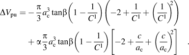
It thus follows that:
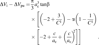
Replacing variable a with a c in Eq. (13):

The volume loss in the plastic zone and elastic zone is calculated starting from  . To simplify the calculation, it is assumed that
 is calculated for a spherical cap defined by the ψ angle shown in Fig. 2(a). It thus follows that:

Replacing variable cosψ with (h c − h)/c leads to
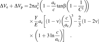
Taking Λ′ defined by Eq. (15) and substituting Eqs. (22), (23), and (25) into Eq. (19) leads to:

When tanβ << 1, Eq. (26) becomes:
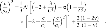
This equation is more complex than the Johnson’s formulation. The determination of the c/a c ratio necessitates the solution of a polynomial equation of degree 3 and the knowledge of the C 1 parameter. Finite element method (FEM) simulations show that the results obtained from Eq. (27) are very close to those obtained from Eq. (26), even for large values of β. Notice that Eq. (27) becomes equal to the Johnson’s formulation [Eq. (5)] if there is no pile-up or sink-in.
B. Materials that exhibit sink-in
The concept of ECM based on the equality between the displaced volumes and the volume loss in the indented material is applied for materials that exhibit sink-in.
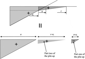
Figure 3 shows that the geometrical constructions proposed to define the pile-up can be used to define the sink-in.
Volume displaced by the indented materials that exhibit sink-in.

In light of this analogy, the volume of the sink-in, i.e., ∆V si, can be determined with Eq. (19) where ∆V pu is replaced by ∆V si. It thus follows that the c/a c ratio is also obtained from Eq. (27) in the case of materials that exhibit sink-in.
V. APPLICATION OF THE NEW ECM
To illustrate the new ECM developed in the preceding section, the constraint factor C f = H/Y obtained by applying Eqs. (18) and (27) is compared with numerical results.
A. FEM model
The finite element analysis presented here assumes a conical perfectly rigid indenter in frictionless contact with the flat surface of the specimen. The simulations were performed in axisymmetric mode using the large strain elastic–plastic feature of the Abaqus finite element code.
For conical indentation of elastic-ideally plastic materials, the degree of indentation is commonly defined by the nondimensional E*tanβ/Y [where E* = E/(1−ν2)].Reference Johnson2 The numerical simulations were performed for various β angles and constant E/Y ratio. The E/Y ratios of the indented materials are equal to 200, 2000, 20,000, and 200,000. The high value of E/Y ratio (200,000) was chosen to obtain a material very similar to the rigid-ideally plastic material for which the similarity regime can be reached. The finite element simulations were performed for materials with Poisson’s values ν = 0, 0.3 and 0.5. The constitutive model of the elastic-ideally plastic indented material was taken to follow the well known J2-associated flow theory with rate-independent deformation. The constraint factor is calculated starting from the weight average of the indentation pressures obtained during the indentation process. The size of the elements in contact with the indenter is equal to 0.003a at maximum penetration depth. Details of the finite element meshes and their density-region hierarchy are given by Bartier and Hernot.Reference Bartier and Hernot17
B. FEM results
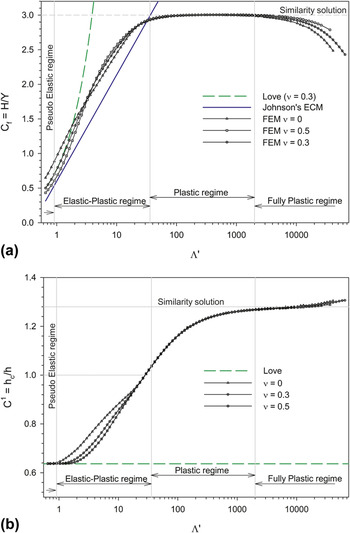
Figure 4 shows the development of C f and C 1 with Λ′. Four regimes are differentiated in this figure. First, up to Λ′ = 0.91, there is no deviation in behavior from the elastic stage described by Love.Reference Love1 This first regime can be called “pseudoelastic regime.” The second regime occurs when the contact pressure lies between approximately 0.7Y and 3Y. This regime corresponds to the elastic–plastic regime defined by Johnson in which the Johnson’s ECM given in Eq. (18) is considered as valid.Reference Johnson2, Reference Johnson8, Reference Studman, Moore and Jones10 The third regime is reached when C f = 3. This regime is commonly called “fully plastic.” Notice that C 1 is not constant in this regime. We will show thereafter that this regime is not fully plastic because the elasticity cannot be considered as negligible. The fourth regime is reached for large values of Λ′ and corresponds to a drop of C f. We will show that this regime is fully plastic.
Evolution of the constraint factor, C f, and C 1 parameter during conical indentation of elastic-ideally plastic material with E/Y = 200,000. (a) C f and (b) C 1.

C. New ECM predictions
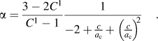
To calculate the radius of the plastic zone from Eq. (27), one has to define the value of the α constant. If the existence of a similarity regime is assumed, it is also assumed that C f and C 1 take constant value during this regime. For materials very similar to the rigid-ideally plastic material, C f and C 1 remain constant for large values of Λ′. In order not to obtain c → ∞ from Eq. (27), it is necessary to verify that:
For Alcala et al.,Reference Alcala, Barone and Anglada18C 1 = 1.202, for Felder,Reference Felder19C 1 = 1.263, for Malherbe et al.,Reference Malherbe, Benayoun, Morel and Iost20C 1 = 1.28, and for Pelletier,Reference Pelletier21C 1 = 1.3. For the proposed study, C 1 was fixed at 1.28 in Eq. (27) (value close to the numerical results).
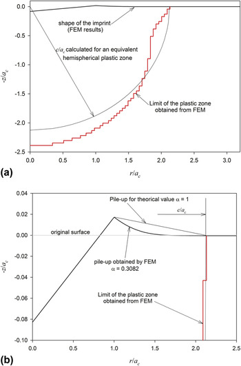
In the Johnson’s ECM,Reference Johnson8Eq. (18) gives the elastic–plastic boundary at c/a c ≈ 2.3 when the “fully plastic” state, defined by C f = 3, occurs. This result matches the experimentally based estimates of Zielinski et al.Reference Zielinski, Huang and Gerberich22 who found that c/a c ≈ 2.12. By assuming that c/a c ≈ 2.2 and C 1 = 1.285, Eq. (28) gives α = 0.3. This value is in agreement with the numerical results obtained for the studied materials. For example, the calculation of the pile-up volume for a material with E/Y = 2,000 and tanβ = 0.1 gives α = 0.3082 (Fig. 5)
(a) Plastic zone and (b) shape of the imprint obtained from finite element method (material with E/Y = 2,000 and tanβ = 0.1).

α = 0.3 was introduced in Eq. (27).
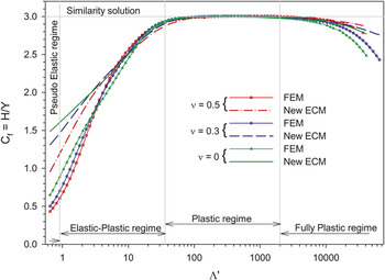
The variation of the normalized indentation pressure (H/Y) with the degree of indentation (Λ′) obtained from Eqs. (18) and (27) is illustrated in Fig. 6.
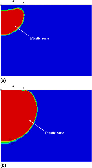
In Fig. 6, H/Y was calculated for the material with E/Y = 200,000. This figure reveals that the theoretical results are in accordance to the finite element simulations in the third indentation regime and in the final portion of the second indentation regime. Figure 7(a) shows that the shape of the plastic zone is very different from the shape described in Fig. 2 at the beginning of the elastic–plastic regime. For Λ′ = 2, the plastic zone remains embedded within an elastic zone. The failure of the assumptions involved in ECM can explain the difference between theoretical results and numerical results at the beginning of the elastic–plastic regime. Figure 7(b) shows that the plastic zone is similar to the shape of the plastic zone described in Fig. 2 when Λ′ = 10. Starting from this value, the predicted constraint factor curve fits well with all numerical data points up to the end of the third indentation regime.
Predictions from the new ECM for conical indentation of elastic-ideally plastic materials with E/Y = 200,000.

Plastic zone in a material, with E/Y = 200,000 and v = 0, indented by cone: (a) Λ′ = 2 and (b) Λ′ = 10.

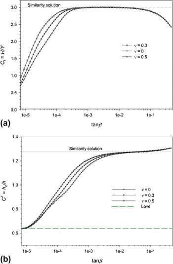
Figure 4(a) shows that the constraint factor remains about constant and close to 3 for Λ′ in the range 36–2000 (third regime). It is commonly assumed that “fully plastic” regime is reached when the constraint factor remains constant during plastic deformation. It is also assumed that “fully plastic” regime occurs when the elastic contribution to the strain field beneath the indenter is negligible, and the parameters E*tanβ/Y or Λ′ cease to uniquely define the degree of indentation. To determine if the elastic contribution to the strain field beneath the indenter is negligible when C f = 3, simulations were performed for materials with values of ν = 0, 0.3, and 0.5.
Figure 4(b) shows that the development of the pile-up is dependent on the Poisson’s ratio when C f = 3. This result shows that Λ′ continues to define the degree of indentation when C f remains constant. Thus, the third regime cannot be considered as “fully plastic.” For this regime, the new ECM has the capacity to describe the indentation test (Fig. 6).
As it was mentioned above, the fourth regime corresponds to a drop of C f. The normalized indentation pressure (H/Y) obtained from the proposed ECM also decreases in the fourth indentation regime, but this decrease is much less pronounced (Fig. 6). Figure 4(b) shows that the decrease in C f corresponds to a steeper increase in the pile-up.
When C f begins to decrease from 3, the C f–Λ′ and C 1–Λ′ curves markedly separate and thus Λ′ is inappropriate to correlate the indention tests on materials of various Poisson’s ratios. Figure 8 shows the existence of unique solution if C f and C 1 are plotted versus tanβ. This indicates that the elastic contribution to the strain field beneath the indenter is negligible for the regime where C f decreases. Thus, this regime can be considered as “fully plastic.” For this regime, the new ECM is inappropriate to describe the indentation test.
Variation of C f and C 1 with tanβ for an elastic-ideally plastic material with E/Y = 200,000. (a) C f and (b) C 1.

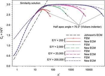
Figure 9 shows the variation of C f, with Λ′ for elastic-ideally plastic materials of various E/Y ratios. This figure shows that with decreasing E/Y ratio the regime where hardness remains constant tends to vanish. The same phenomenon was observed in the case of spherical indentation of elastic-ideally plastic materials.Reference Bartier and Hernot17
Predictions from the new ECM for conical indentation of various elastic-ideally plastic materials.

As shown above, the regime where C f decays is fully plastic. The existence of the fully plastic regime is due to the high values of the plastic strain located in periphery of the contact and to the greatest facility of material displacement on the surface. The combination of these two phenomena has as a consequence a decrease in the mean contact pressure and a higher increase in the pile-up (Fig. 4). Figure 9 also shows that for a given apical angle of the tip, C f becomes constant irrespectively of Λ′ if fully plastic regime is reached. For our conditions, C f ≈ 2.54 if a Vickers indenter with an equivalent conical tip half apex angle of 70:3° is used. Notice that C f will be higher than this value in fully plastic regime for friction contact and strain hardening materials.Reference Mata and Alcala23, Reference Gao24 As for the elastic-ideally plastic material of large E/Y ratio, ECM does not match numerical results in the regime where C f decays (Fig. 9). We can notice however that the new ECM gives better results than the Johnson’s ECM because pile-up or sink-in is taken into account.
VI. CONCLUSION
A new ECM for describing conical indentation of elastic-ideally plastic material was proposed in this article. We show that the Johnson’s ECM based on the conservation of volume during an increment of penetration can be replaced by an ECM based on the equality between the displaced volumes and the volume loss in the indented material. For the proposed ECM, it is assumed that the volume of material displaced by the indenter is equal to the volume loss, due to elastic deformation, in the material and depends on the pile-up or sink-in. It was shown that the proposed ECM results match very well with the numerical data in the final portion of the transition regime for which the contact pressure lies between approximately 2.5Y and 3Y. For material of large E/Y ratio, the new ECM also provides results which are very close to the numerical data in the plastic-similarity regime (regime in which C f = 3). It is commonly assumed that this last regime is “fully plastic.” We show that it is not the case because the elastic contribution to the strain field beneath the indenter is nonnegligible in this regime. For material of smaller E/Y ratio, the proposed ECM gives better results than the Johnson’s ECM because pile-up or sink-in is taken into account.