1 Introduction
The impulsive acceleration of a perturbed interface separating fluids of different densities, typically due to a shock wave traversing the interface, results in growth of the interfacial perturbations. This instability, first considered by Markstein (Reference Markstein1957), was studied theoretically by Richtmyer (Reference Richtmyer1960) and experimentally by Meshkov (Reference Meshkov1969). Consequently it is known as the Richtmyer–Meshkov instability (RMI).
The RMI occurs in a variety of applications, as discussed in the review of Brouillette (Reference Brouillette2002): in astrophysics, it has been used to explain the lack of stratification in supernova products and is required in stellar evolution models (Arnett Reference Arnett2000); in combustion systems with shock–flame interactions, it plays on important role in deflagration-to-detonation transition (Khokhlov, Oran & Thomas Reference Khokhlov, Oran and Thomas1999); it can be used to promote mixing in supersonic air-breathing engines (Yang, Kubota & Zukoski Reference Yang, Kubota and Zukoski1993); and is a possible mechanism for test flow contamination by driver gas in shock tunnels (Stalker & Crane Reference Stalker and Crane1978; Brouillette & Bonazza Reference Brouillette and Bonazza1999). The application that has motivated the majority of studies is inertial confinement fusion (ICF), a technology with the potential to demonstrate highly efficient carbon-free energy production (Glenzer et al. Reference Glenzer, MacGowan, Michel, Meezan, Suter, Dixit, Kline, Kyrala, Bradley and Callahan2010). In ICF, a spherically converging shock is driven into a target capsule containing fuel, generating conditions at the centre sufficient to initiate fusion. The RMI of the material interfaces in ICF targets limits chance of achieving energy break-even or production (Lindl, McCrory & Campbell Reference Lindl, McCrory and Campbell1992; Lindl et al. Reference Lindl, Landen, Edwards, Moses, Adams, Amendt, Antipa, Arnold, Atherton and Azevedo2014). Consequently, there has been a recent focus on the converging shock-driven RMI in both gases (Lanier et al. Reference Lanier, Barnes, Batha, Day, Magelssen, Scott, Dunne, Parker and Rothman2003; Hosseini & Takayama Reference Hosseini and Takayama2005; Mikaelian Reference Mikaelian2005; Lombardini, Pullin & Meiron Reference Lombardini, Pullin and Meiron2014a ,Reference Lombardini, Pullin and Meiron b ) and solids (López Ortega et al. Reference López Ortega, Lombardini, Pullin and Meiron2014, Reference López Ortega, Lombardini, Barton, Pullin and Meiron2015). It is also important to note that in ICF, the materials involved become rapidly ionised, and hence will interact with magnetic fields.
It has been demonstrated, through both experiments (Manuel et al. Reference Manuel, Li, Séguin, Frenje, Casey, Petrasso, Hu, Betti, Hager and Meyerhofer2012a ; Séguin et al. Reference Séguin, Li, Manuel, Rinderknecht, Sinenian, Frenje, Rygg, Hicks, Petrasso and Delettrez2012; Igumenshchev et al. Reference Igumenshchev, Zylstra, Li, Nilson, Goncharov and Petrasso2014) and Hall magnetohydrodynamic (MHD) simulations including the Biermann battery effect (Srinivasan, Dimonte & Tang Reference Srinivasan, Dimonte and Tang2012), that self-generated magnetic fields arise in ICF implosions. Such self-generated fields are thought to influence ICF implosions through mechanisms such as reduced electron thermal conduction (Srinivasan et al. Reference Srinivasan, Dimonte and Tang2012). Depending on the location where strong fields are present, reduced electron thermal conduction may be beneficial by reducing heat losses from the hot spot (Hohenberger et al. Reference Hohenberger, Chang, Fiskel, Knauer, Betti, Marshall, Meyerhofer, Séguin and Petrasso2012) or detrimental by reducing the coupling efficiency between the drive laser energy and the ablating capsule (Manuel et al. Reference Manuel, Li, Séguin, Frenje, Casey, Petrasso, Hu, Betti, Hager and Meyerhofer2012b ). One framework for modelling the coupled evolution of plasmas and magnetic fields is ideal MHD. In this framework, its has been demonstrated that the planar RMI is suppressed in the presence of initial magnetic fields that are either normal (Samtaney Reference Samtaney2003; Wheatley, Samtaney & Pullin Reference Wheatley, Samtaney and Pullin2005, Reference Wheatley, Samtaney and Pullin2009) or tangential (Cao et al. Reference Cao, Wu, Ren and Li2008; Wheatley et al. Reference Wheatley, Samtaney, Pullin and Gehre2014) to the interface. This magnetic suppression of the RMI, combined with that of the Rayleigh–Taylor instability (RTI) (Chandrasekhar Reference Chandrasekhar1961), have recently been computationally investigated for converging cases (Mostert et al. Reference Mostert, Wheatley, Samtaney and Pullin2015, Reference Mostert, Pullin, Wheatley and Samtaney2017), and are likely contributing factors to the observations of Perkins et al. (Reference Perkins, Logan, Zimmerman and Werner2013).
Two requirements for the single-fluid MHD model to be valid are that the plasma length scales known as the Debye length and the Larmor radius are small compared to the length scales characterising the problem under consideration. In the magnetised implosion experiments of Hohenberger et al. (Reference Hohenberger, Chang, Fiskel, Knauer, Betti, Marshall, Meyerhofer, Séguin and Petrasso2012), it was determined that the alpha particle Larmor radius was larger than the hot-spot size. Thus there are circumstances in ICF-like implosions when at least one of the plasma length scales must be considered finite, and the single-fluid MHD model is not appropriate. One continuum, fluid-based model that permits finite plasma length scales is defined by the ideal two-fluid, ion–electron, continuum plasma equations. These couple a separate set of conservation equations for each species to the full Maxwell equations for the evolution of the electromagnetic fields. These equations allow the effects of charge separation to be accounted for, including electric fields exerting a net body force, and will be shown to intrinsically include the self-generation of magnetic fields through the Biermann battery and other effects, unlike the equations of hydrodynamics or MHD. The effects of electron inertia and a finite speed of light are included, unlike in Hall MHD. We will collectively refer to the phenomena modelled by the two-fluid system that are precluded in single-fluid MHD as two-fluid effects.
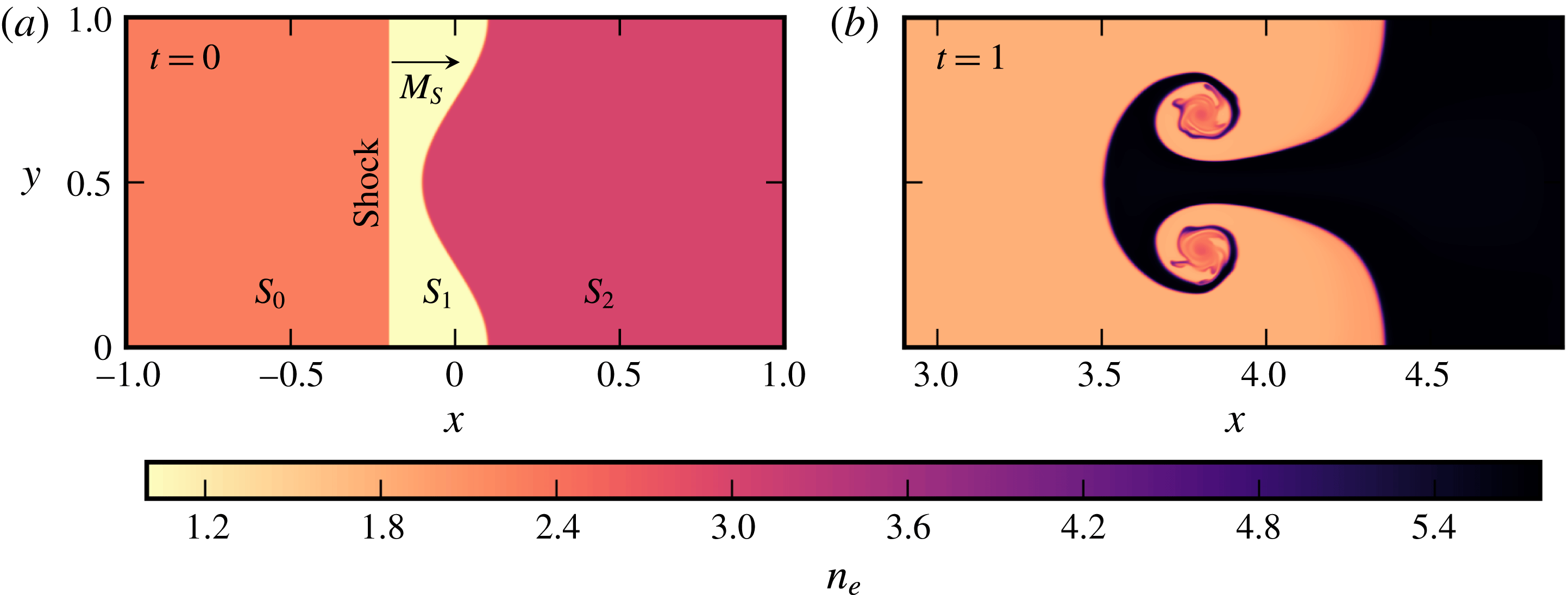
Initial conditions for simulations of the single-mode thermal RMI (a) and a nonlinear, evolved solution for a neutral species corresponding to the electron fluid (b). Contours of electron number density
 $n_{e}$
are shown.

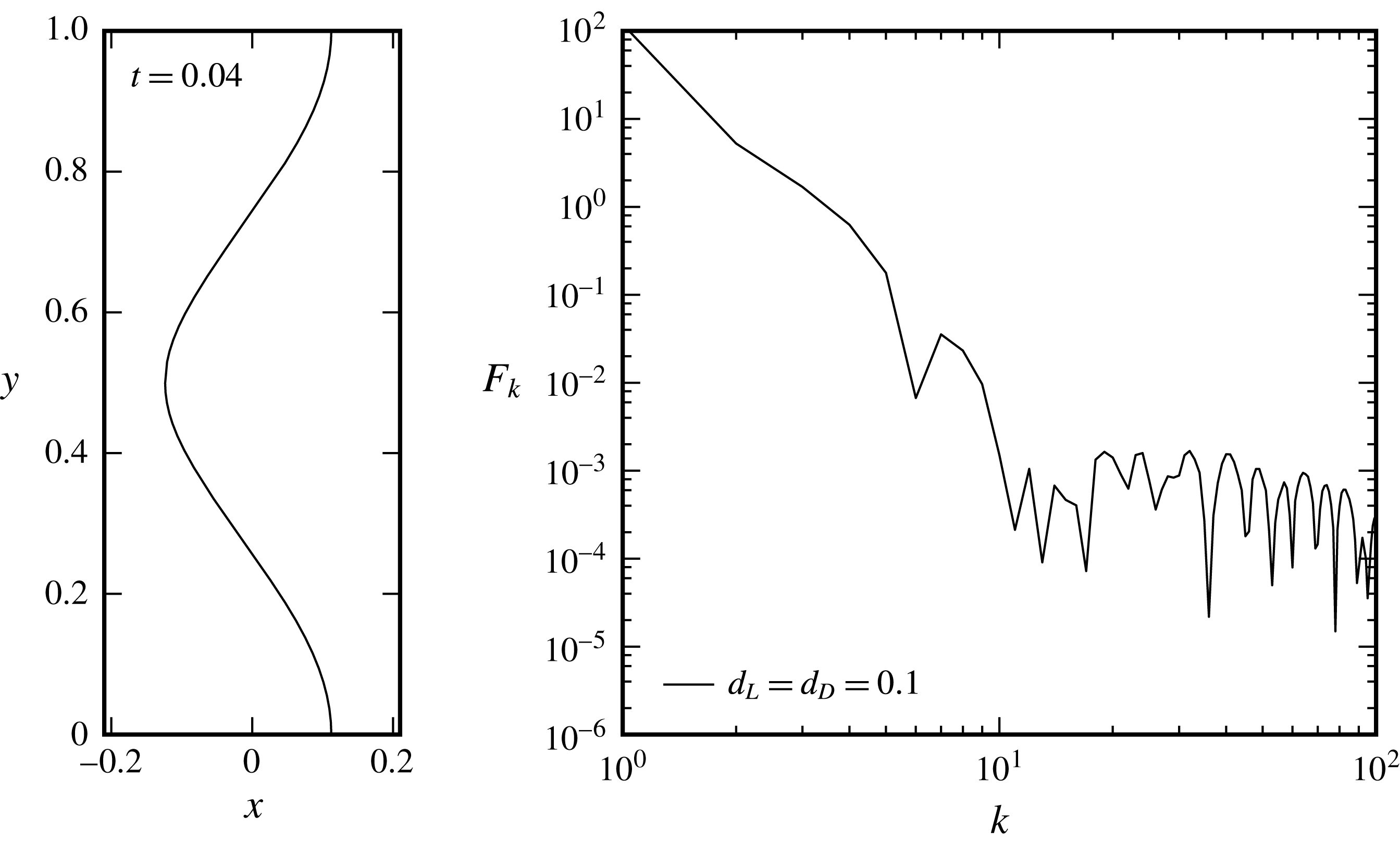
The present study is a fundamental investigation of the influence two-fluid effects can have on the initially unmagnetised plasma RMI. For this reason, we study the canonical planar, single-mode RMI for plasma parameters where two-fluid effects are expected to be significant. The initial condition for this flow are shown in figure 1. In the present work we study the case where the initial density jump across the perturbed interface is due to a temperature discontinuity, rather than an ion species discontinuity. Both situations are physically relevant in ICF; temperature discontinuities in the same species may occur, for example, between fuel that was initially frozen and that which was initially vapour in a cryogenic target, while species discontinuities occur between the shell material and the fuel. In hydrodynamics and single-fluid MHD, the RMIs of thermal and species discontinuities with identical density ratios behave similarly. In the two-fluid plasma case, there is a significant difference; for a thermal interface, there is a density jump in the electrons, while for an ion species interface there is not. The presence of an electron density interface in the former case is anticipated to yield more complex behaviour, and hence is where we focus our attention.
The remainder of the paper is organised as follows: The system of equations to be simulated is presented in § 2 along with the link between vorticity and self-generated magnetic fields. The numerical implementation of these equations is also briefly discussed. Verification of the numerical solver is performed in § 3. Section 4 describes the initial conditions for the primary simulations performed in this study. Investigation of the one-dimensional flow underlying the two-fluid plasma RMI is then carried out in § 5, followed by the results of two-dimensional RMI simulations in § 6. The discussion and analysis of the results focuses on the phenomena present in the flow that are absent in the single-fluid model and the effects these have on the growth of interface perturbations. The occurrence of self-generated magnetic fields is noted, but as these are not our focus, they will be investigated in greater depth elsewhere. Finally, conclusions are given in § 7.
2 The two-fluid plasma model
The two-fluid Euler equations for the ions and electrons with appropriate electromagnetic forcing terms are (Loverich Reference Loverich2003),
 $$\begin{eqnarray}\displaystyle & \displaystyle \frac{\unicode[STIX]{x2202}\unicode[STIX]{x1D70C}_{\unicode[STIX]{x1D6FC}}}{\unicode[STIX]{x2202}t}+\unicode[STIX]{x1D735}\boldsymbol{\cdot }(\unicode[STIX]{x1D70C}_{\unicode[STIX]{x1D6FC}}\boldsymbol{u}_{\unicode[STIX]{x1D6FC}})=0, & \displaystyle\end{eqnarray}$$
 $$\begin{eqnarray}\displaystyle & \displaystyle \frac{\unicode[STIX]{x2202}\unicode[STIX]{x1D70C}_{\unicode[STIX]{x1D6FC}}\boldsymbol{u}_{\unicode[STIX]{x1D6FC}}}{\unicode[STIX]{x2202}t}+\unicode[STIX]{x1D735}\boldsymbol{\cdot }(\unicode[STIX]{x1D70C}_{\unicode[STIX]{x1D6FC}}\boldsymbol{u}_{\unicode[STIX]{x1D6FC}}\boldsymbol{u}_{\unicode[STIX]{x1D6FC}}+p_{\unicode[STIX]{x1D6FC}}\boldsymbol{I})=n_{\unicode[STIX]{x1D6FC}}q_{\unicode[STIX]{x1D6FC}}(\boldsymbol{E}+\boldsymbol{u}_{\unicode[STIX]{x1D6FC}}\times \boldsymbol{B}), & \displaystyle\end{eqnarray}$$
 $$\begin{eqnarray}\displaystyle & \displaystyle \frac{\unicode[STIX]{x2202}\unicode[STIX]{x1D716}_{\unicode[STIX]{x1D6FC}}}{\unicode[STIX]{x2202}t}+\unicode[STIX]{x1D735}\boldsymbol{\cdot }((\unicode[STIX]{x1D716}_{\unicode[STIX]{x1D6FC}}+p_{\unicode[STIX]{x1D6FC}})\boldsymbol{u}_{\unicode[STIX]{x1D6FC}})=n_{\unicode[STIX]{x1D6FC}}q_{\unicode[STIX]{x1D6FC}}\boldsymbol{u}_{\unicode[STIX]{x1D6FC}}\boldsymbol{\cdot }\boldsymbol{E}, & \displaystyle\end{eqnarray}$$
where,
 $$\begin{eqnarray}\displaystyle \unicode[STIX]{x1D70C}_{\unicode[STIX]{x1D6FC}}=n_{\unicode[STIX]{x1D6FC}}m_{\unicode[STIX]{x1D6FC}},\quad p_{\unicode[STIX]{x1D6FC}}=n_{\unicode[STIX]{x1D6FC}}k_{B}T_{\unicode[STIX]{x1D6FC}},\quad \unicode[STIX]{x1D716}_{\unicode[STIX]{x1D6FC}}=\frac{p_{\unicode[STIX]{x1D6FC}}}{\unicode[STIX]{x1D6FE}_{\unicode[STIX]{x1D6FC}}-1}+\frac{\unicode[STIX]{x1D70C}_{\unicode[STIX]{x1D6FC}}|\boldsymbol{u}_{\unicode[STIX]{x1D6FC}}|^{2}}{2}. & & \displaystyle\end{eqnarray}$$
Here, the subscript
 $\unicode[STIX]{x1D6FC}$
denotes the species with
 $\unicode[STIX]{x1D70C}_{\unicode[STIX]{x1D6FC}}$
the species density,
 $n_{\unicode[STIX]{x1D6FC}}$
the number density and
 $m_{\unicode[STIX]{x1D6FC}}$
the particle mass. The species energy is
 $\unicode[STIX]{x1D716}_{\unicode[STIX]{x1D6FC}}$
, velocity is
 $\boldsymbol{u}_{\unicode[STIX]{x1D6FC}}=(u_{\unicode[STIX]{x1D6FC}},v_{\unicode[STIX]{x1D6FC}},w_{\unicode[STIX]{x1D6FC}})^{\text{T}}$
while pressure and temperature are
 $p_{\unicode[STIX]{x1D6FC}}$
and
 $T_{\unicode[STIX]{x1D6FC}}$
respectively. The ratio of specific heats is
 $\unicode[STIX]{x1D6FE}_{\unicode[STIX]{x1D6FC}}$
and
 $k_{B}$
is the Boltzmann constant. Each species is in its own kinetic-collisional equilibrium, neglecting inter-species collisions. This is justified by the relaxation rate for interspecies collisional equilibration typically being orders of magnitude slower than for the individual species, often causing plasmas to be in partial thermodynamic equilibrium only within the constituent species (Bellan Reference Bellan2006). The species interact via the induced electric
 $\boldsymbol{E}$
and magnetic
 $\boldsymbol{B}$
fields according to Maxwell’s equations,
 $$\begin{eqnarray}\displaystyle & \displaystyle \frac{\unicode[STIX]{x2202}\boldsymbol{B}}{\unicode[STIX]{x2202}t}+\unicode[STIX]{x1D735}\times \boldsymbol{E}=0, & \displaystyle\end{eqnarray}$$
 $$\begin{eqnarray}\displaystyle & \displaystyle \frac{\unicode[STIX]{x2202}\boldsymbol{E}}{\unicode[STIX]{x2202}t}-c^{2}\unicode[STIX]{x1D735}\times \boldsymbol{B}=-\frac{1}{\unicode[STIX]{x1D716}_{0}}\mathop{\sum }_{\unicode[STIX]{x1D6FC}}n_{\unicode[STIX]{x1D6FC}}q_{\unicode[STIX]{x1D6FC}}\boldsymbol{u}_{\unicode[STIX]{x1D6FC}}, & \displaystyle\end{eqnarray}$$
 $$\begin{eqnarray}\displaystyle & \displaystyle \unicode[STIX]{x1D735}\boldsymbol{\cdot }\boldsymbol{E}=\frac{1}{\unicode[STIX]{x1D716}_{0}}\mathop{\sum }_{\unicode[STIX]{x1D6FC}}r_{\unicode[STIX]{x1D6FC}}\unicode[STIX]{x1D70C}_{\unicode[STIX]{x1D6FC}}, & \displaystyle\end{eqnarray}$$
 $$\begin{eqnarray}\displaystyle & \displaystyle \unicode[STIX]{x1D735}\boldsymbol{\cdot }\boldsymbol{B}=0, & \displaystyle\end{eqnarray}$$
where the speed of light
 $c$
is given by
 $c^{2}=(1/\unicode[STIX]{x1D707}_{0}\unicode[STIX]{x1D716}_{0})$
with permeability of free space
 $\unicode[STIX]{x1D707}_{0}$
and vacuum permittivity
 $\unicode[STIX]{x1D716}_{0}$
. These equations are non-dimensionalised by specifying a reference length scale
 $x_{0}$
, Larmor radius
 $d_{L}$
, Debye length
 $d_{D}$
and non-dimensional light speed
 ${\hat{c}}=c/u_{0}$
(the reference velocity
 $u_{0}$
is a fixed fraction of
 $c$
). In the initially unmagnetised flows considered presently, the Larmor radius is provided solely to define a reference magnetic field strength and thus allow the self-generated electromagnetic fields to be interpreted in a consistent manner. The reference time
 $t_{0}=x_{0}/u_{0}$
, magnetic field strength
 $B_{0}=(m_{0}u_{0}/q_{0}d_{L})$
, electric field strength
 $E_{0}=cB_{0}$
and number density
 $n_{0}=(\unicode[STIX]{x1D716}_{0}u_{0}^{2}m_{0}/d_{D}^{2}q_{0}^{2})$
are then derived accordingly. Here,
 $q_{0}$
is the charge of an electron
 $e$
and
 $m_{0}$
is the reference mass. This non-dimensionalisation follows Loverich (Reference Loverich2003) and allows the plasma regime to be dictated through the reference
 $d_{L}$
and
 $d_{D}$
. We note that the local plasma length scales in the simulations presented subsequently can vary significantly from the reference values. In particular, for the initially unmagnetised RMI problems considered, the local Larmor radius will only approach
 $d_{L}$
if the ratio of the local non-dimensional velocity and self-generated magnetic field is of order unity. All quantities presented subsequently are non-dimensional.
The final non-dimensional fluid species equations used in the simulations are,
 $$\begin{eqnarray}\displaystyle & \displaystyle \frac{\unicode[STIX]{x2202}\unicode[STIX]{x1D70C}_{\unicode[STIX]{x1D6FC}}}{\unicode[STIX]{x2202}t}+\unicode[STIX]{x1D735}\boldsymbol{\cdot }\left(\unicode[STIX]{x1D70C}_{\unicode[STIX]{x1D6FC}}\boldsymbol{u}_{\unicode[STIX]{x1D6FC}}\right)=0, & \displaystyle\end{eqnarray}$$
 $$\begin{eqnarray}\displaystyle & \displaystyle \frac{\unicode[STIX]{x2202}\unicode[STIX]{x1D70C}_{\unicode[STIX]{x1D6FC}}\boldsymbol{u}_{\unicode[STIX]{x1D6FC}}}{\unicode[STIX]{x2202}t}+\unicode[STIX]{x1D735}\boldsymbol{\cdot }\left(\unicode[STIX]{x1D70C}_{\unicode[STIX]{x1D6FC}}\boldsymbol{u}_{\unicode[STIX]{x1D6FC}}\boldsymbol{u}_{\unicode[STIX]{x1D6FC}}+p_{\unicode[STIX]{x1D6FC}}\boldsymbol{I}\right)=\frac{n_{\unicode[STIX]{x1D6FC}}q_{\unicode[STIX]{x1D6FC}}}{d_{L}}\left(c\boldsymbol{E}+\boldsymbol{u}_{\unicode[STIX]{x1D6FC}}\times \boldsymbol{B}\right), & \displaystyle\end{eqnarray}$$
 $$\begin{eqnarray}\displaystyle & \displaystyle \frac{\unicode[STIX]{x2202}\unicode[STIX]{x1D716}_{\unicode[STIX]{x1D6FC}}}{\unicode[STIX]{x2202}t}+\unicode[STIX]{x1D735}\boldsymbol{\cdot }\left(\left(\unicode[STIX]{x1D716}_{\unicode[STIX]{x1D6FC}}+p_{\unicode[STIX]{x1D6FC}}\right)\boldsymbol{u}_{\unicode[STIX]{x1D6FC}}\right)=\frac{n_{\unicode[STIX]{x1D6FC}}q_{\unicode[STIX]{x1D6FC}}c}{d_{L}}\boldsymbol{u}_{\unicode[STIX]{x1D6FC}}\boldsymbol{\cdot }\boldsymbol{E}. & \displaystyle\end{eqnarray}$$
To reduce the error in the electromagnetic divergence conditions, equations (2.7) and (2.8), introduced by the discretisation necessitated by numerical implementation, the purely hyperbolic form of Maxwell’s equations (PHM) are used (Munz, Ommes & Schneider Reference Munz, Ommes and Schneider2000). The non-dimensional forms of the PHM equations are given by,
 $$\begin{eqnarray}\displaystyle & \displaystyle \frac{\unicode[STIX]{x2202}\boldsymbol{B}}{\unicode[STIX]{x2202}t}+c\left(\unicode[STIX]{x1D735}\times \boldsymbol{E}+\unicode[STIX]{x1D6E4}_{B}\unicode[STIX]{x1D735}\unicode[STIX]{x1D713}_{B}\right)=0, & \displaystyle\end{eqnarray}$$
 $$\begin{eqnarray}\displaystyle & \displaystyle \frac{\unicode[STIX]{x2202}\boldsymbol{E}}{\unicode[STIX]{x2202}t}-c\left(\unicode[STIX]{x1D735}\times \boldsymbol{B}-\unicode[STIX]{x1D6E4}_{E}\unicode[STIX]{x1D735}\unicode[STIX]{x1D713}_{E}\right)=-\frac{d_{L}}{d_{D}^{2}c}\mathop{\sum }_{\unicode[STIX]{x1D6FC}}n_{\unicode[STIX]{x1D6FC}}q_{\unicode[STIX]{x1D6FC}}\boldsymbol{u}_{\unicode[STIX]{x1D6FC}}, & \displaystyle\end{eqnarray}$$
 $$\begin{eqnarray}\displaystyle & \displaystyle \frac{\unicode[STIX]{x2202}\unicode[STIX]{x1D713}_{E}}{\unicode[STIX]{x2202}t}+c\unicode[STIX]{x1D6E4}_{E}\unicode[STIX]{x1D735}\boldsymbol{\cdot }\boldsymbol{E}=\unicode[STIX]{x1D6E4}_{E}\frac{d_{L}}{d_{D}^{2}}\mathop{\sum }_{\unicode[STIX]{x1D6FC}}n_{\unicode[STIX]{x1D6FC}}q_{\unicode[STIX]{x1D6FC}}, & \displaystyle\end{eqnarray}$$
 $$\begin{eqnarray}\displaystyle & \displaystyle \frac{\unicode[STIX]{x2202}\unicode[STIX]{x1D713}_{B}}{\unicode[STIX]{x2202}t}+c\unicode[STIX]{x1D6E4}_{B}\unicode[STIX]{x1D735}\boldsymbol{\cdot }\boldsymbol{B}=0. & \displaystyle\end{eqnarray}$$
In these equations
 $\unicode[STIX]{x1D713}_{E}$
and
 $\unicode[STIX]{x1D713}_{B}$
are Lagrange multipliers introduced to drive errors in the divergence of the fields to zero whilst maintaining a purely hyperbolic formulation. The effectiveness of the Lagrange multiplier method is dictated by the positive dimensionless parameters
 $\unicode[STIX]{x1D6E4}_{E}$
and
 $\unicode[STIX]{x1D6E4}_{B}$
, which determine the speed at which the correction factors are propagated by the system (Munz et al.
Reference Munz, Ommes and Schneider2000). The initial value of
 $\unicode[STIX]{x1D713}_{E}$
and
 $\unicode[STIX]{x1D713}_{B}$
is always zero throughout the domain, the correction potentials are thus generated on demand according to equations (2.14) and (2.15). The effectiveness of this method in controlling divergence errors in the present simulations is documented in appendix A.
2.1 Vorticity and magnetic field self-generation
The vorticity (
 $\unicode[STIX]{x1D74E}$
) equation can be derived by taking the curl of the velocity evolution equation, obtained via (2.10), thus giving,
 $$\begin{eqnarray}\frac{\unicode[STIX]{x2202}\unicode[STIX]{x1D74E}_{\unicode[STIX]{x1D6FC}}}{\unicode[STIX]{x2202}t}-\unicode[STIX]{x1D735}\times (\boldsymbol{u}_{\unicode[STIX]{x1D6FC}}\times \unicode[STIX]{x1D74E}_{\unicode[STIX]{x1D6FC}})-\frac{1}{\unicode[STIX]{x1D70C}_{\unicode[STIX]{x1D6FC}}^{2}}\left(\unicode[STIX]{x1D735}\unicode[STIX]{x1D70C}_{\unicode[STIX]{x1D6FC}}\times \unicode[STIX]{x1D735}p_{\unicode[STIX]{x1D6FC}}\right)=\unicode[STIX]{x1D735}\times \left(\frac{q_{\unicode[STIX]{x1D6FC}}}{d_{L}m_{\unicode[STIX]{x1D6FC}}}\left(c\boldsymbol{E}+\boldsymbol{u}_{\unicode[STIX]{x1D6FC}}\times \boldsymbol{B}\right)\right).\end{eqnarray}$$
From (2.12), where the divergence mitigation terms have been omitted (
 $\unicode[STIX]{x1D6E4}_{B}=0$
), we see that
 $(\unicode[STIX]{x2202}\boldsymbol{B}/\unicode[STIX]{x2202}t)=-c\unicode[STIX]{x1D735}\times \boldsymbol{E}$
which leads to
 $$\begin{eqnarray}\frac{\unicode[STIX]{x2202}\boldsymbol{B}}{\unicode[STIX]{x2202}t}=\frac{d_{L}}{q_{\unicode[STIX]{x1D6FC}}m_{\unicode[STIX]{x1D6FC}}}\left(\frac{1}{n_{\unicode[STIX]{x1D6FC}}^{2}}\unicode[STIX]{x1D735}\unicode[STIX]{x1D70C}_{\unicode[STIX]{x1D6FC}}\times \unicode[STIX]{x1D735}p_{\unicode[STIX]{x1D6FC}}-\frac{\unicode[STIX]{x2202}\unicode[STIX]{x1D74E}_{\unicode[STIX]{x1D6FC}}}{\unicode[STIX]{x2202}t}+\unicode[STIX]{x1D735}\times \left(\boldsymbol{u}_{\unicode[STIX]{x1D6FC}}\times \unicode[STIX]{x1D74E}_{\unicode[STIX]{x1D6FC}}\right)\right)+\unicode[STIX]{x1D735}\times \left(\boldsymbol{u}_{\unicode[STIX]{x1D6FC}}\times \boldsymbol{B}\right).\end{eqnarray}$$
Here, the first term on the right-hand side is the so-called Biermann battery effect (Schluter & Biermann Reference Schluter and Biermann1950), considered to be the source of self-generated magnetic fields. This shows that self-generated magnetic fields are intrinsic to the two-fluid plasma equations, and that the Biermann battery source term is directly proportional to the baroclinic generation of fluid vorticity, as is the case in the single-fluid model with a generalised Ohm’s law (Evans Reference Evans1986). The link between fluid vorticity and self-generated magnetic fields in the two-fluid model is not explored in depth here as our focus is on the influence of two-fluid effects on the RMI.
2.2 Numerical implementation
Numerical solutions were obtained in one- and two-space dimensions using the adaptive mesh refinement (AMR) framework Chombo (Adams et al. Reference Adams, Colella, Graves, Johnson, Keen, Ligocki, Martin, McCorquodale, Modiano and Schwartz2015). The base numerical method consists of a spatially second-order accurate finite-volume scheme with a two-stage, second-order Runge–Kutta time integrator (Gottlieb, Shu & Tadmor Reference Gottlieb, Shu and Tadmor2001) with minmod limited interface values for flux calculation. Species and electromagnetic fluxes are calculated with the HLLC (Harten–Lax–van Leer–Contact) (Toro, Spruce & Speares Reference Toro, Spruce and Speares1994) and HLLE (Harten–Lax–van Leer–Einfeldt) (Einfeldt Reference Einfeldt1988) approximate Riemann solvers, respectively. The contribution from source terms is solved locally with the implicit method of Abgrall & Kumar (Reference Abgrall and Kumar2014). In order to track the density interface present in the RMI simulations a volume-of-fluid approach is used.
3 Solver verification
3.1 Spatial convergence
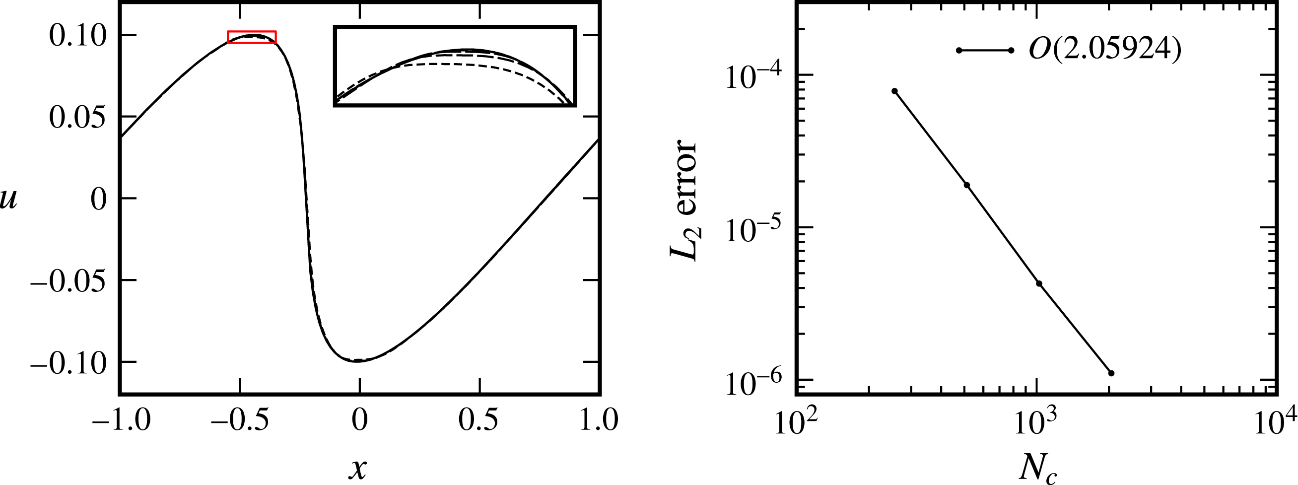
Attaining the prescribed spatial order of convergence of a numerical method is an important component in the verification of a numerical implementation. According to § 2.2, convergence of second order is expected in smooth regions of the flow for the solver used in this work. This convergence rate is verified by calculating solutions to the steepening wave problem of Landau & Lifshitz (Reference Landau and Lifshitz1987) and comparing these numerical solutions to the analytical solution. The steepening wave problem is an initially smooth nonlinear process whereby a sinusoidally perturbed flow field steepens to form a discontinuity at time
 $t_{b}=|2/(u_{0}\unicode[STIX]{x03C0}(\unicode[STIX]{x1D6FE}+1))|$
. The test case, as implemented, consists of a one-dimensional flow domain
 $-1\leqslant x\leqslant 1$
, periodic in
 $x$
and
 $y$
, with initial conditions
 $$\begin{eqnarray}\displaystyle & \displaystyle u=u_{0}\sin \unicode[STIX]{x03C0}x, & \displaystyle\end{eqnarray}$$
 $$\begin{eqnarray}\displaystyle & \displaystyle \unicode[STIX]{x1D70C}=\unicode[STIX]{x1D70C}_{0}\left(1+\frac{\left(\unicode[STIX]{x1D6FE}-1\right)u}{2a_{0}}\right)^{(2/\unicode[STIX]{x1D6FE}-1)}, & \displaystyle\end{eqnarray}$$
 $$\begin{eqnarray}\displaystyle & \displaystyle p=p_{0}\left(1+\frac{\left(\unicode[STIX]{x1D6FE}-1\right)u}{2a_{0}}\right)^{(2\unicode[STIX]{x1D6FE}/\unicode[STIX]{x1D6FE}-1)}, & \displaystyle\end{eqnarray}$$
where
 $u_{0}=0.1$
,
 $\unicode[STIX]{x1D70C}_{0}=1$
,
 $p_{0}=1$
,
 $\unicode[STIX]{x1D6FE}=(5/3)$
and
 $a_{0}$
is the sound speed. Solutions for the velocity field at a time of
 $t=0.9t_{b}$
are shown in figure 2, where the convergence rate is shown to be slightly greater than two (2.06) when calculated over an order of magnitude change in grid resolution. Practically identical results are also obtained for the pressure and density fields and are thus not shown for the sake of brevity. From this result, the underlying fluid solver used to evolve the two-fluid system of equations is shown to perform as expected.
Comparison of the velocity field to analytical solution of the nonlinear steepening wave problem at
 $t=0.9t_{b}$
.

3.2 Solver components
As the two-fluid system of equations is a combination of the electromagnetically forced Euler and Maxwell equations, it is desirable to verify each component of the solver in isolation as well as in combination. This process also allows a relatively rigorous approach due to the lack of accepted benchmarks for the two-fluid system of equations. By setting the charge of each fluid species to zero (
 $q_{i}=q_{e}=0$
), or by setting the plasma length scales to infinity (
 $d_{L}=d_{D}=\infty$
), the two-fluid equations reduce to Euler’s and Maxwell’s equations in isolation. We thus define a Riemann problem centred at
 $x=0$
for the fluid species with left state
 $S_{0}$
and right state
 $S_{1}$
(see (4.2)) while the initial conditions for the electromagnetic fields are
 $$\begin{eqnarray}\displaystyle \left(\begin{array}{@{}c@{}}B_{x},\,B_{z}\\ B_{y}\\ \boldsymbol{E}\end{array}\right)_{L}=\left(\begin{array}{@{}c@{}}0.0\\ -1.0\\ \mathbf{0}\end{array}\right),\quad \left(\begin{array}{@{}c@{}}B_{x},\,B_{z}\\ B_{y}\\ \boldsymbol{E}\end{array}\right)_{R}=\left(\begin{array}{@{}c@{}}0.0\\ 1.0\\ \mathbf{0}\end{array}\right). & & \displaystyle\end{eqnarray}$$
The non-dimensional speed of light for this test is
 $c=10$
while all other properties are as given in § 4.
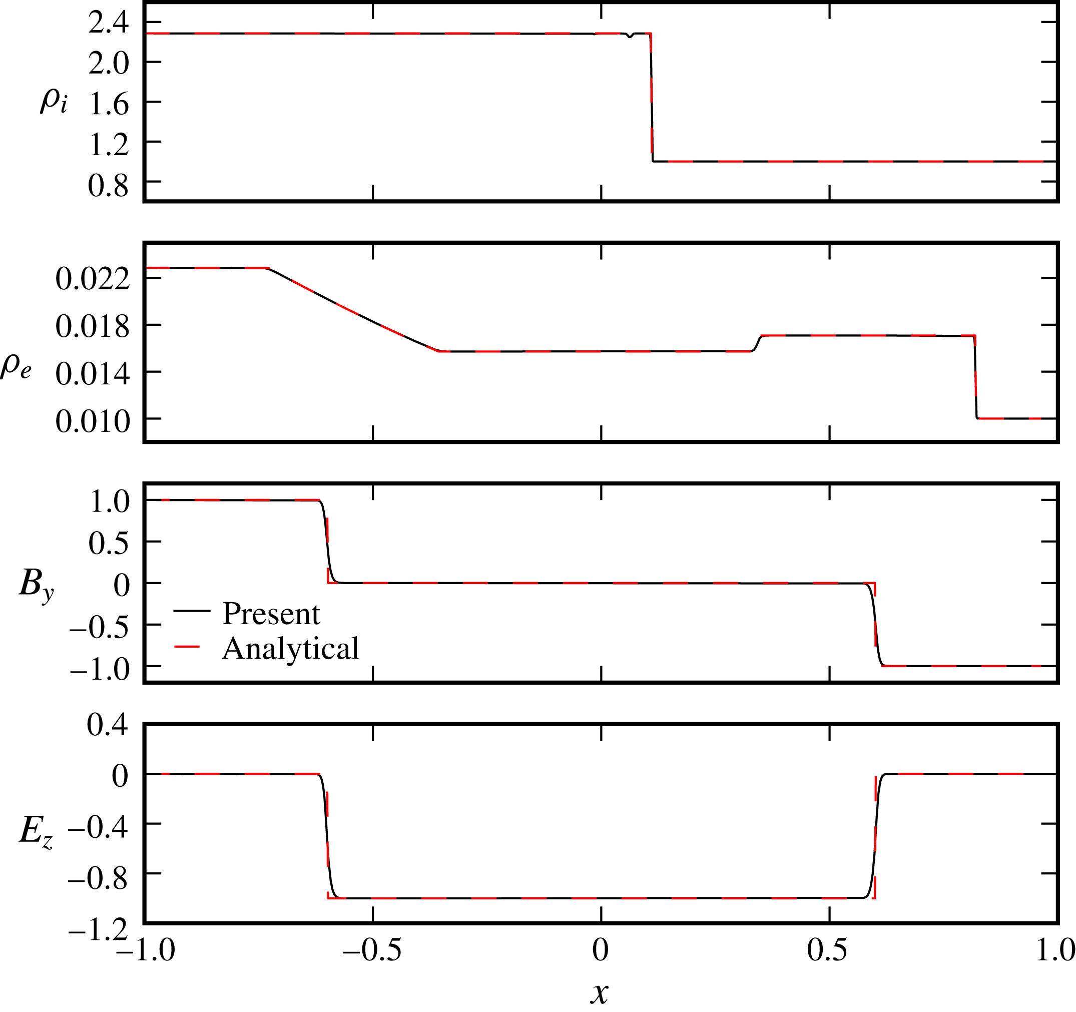
Comparison of simulation results to analytical solutions at
 $t=0.06$
.

The numerical solution to this initial value problem is compared to the analytical solution in figure 3 at a time of
 $t=0.06$
with 2048 cells per unit length. From these results the Euler and Maxwell solvers are shown to capture the analytical solution quite closely with mean
 $L_{2}$
error
 ${<}10^{-3}$
for all cases. The density profile showing the ion shock exhibits a slight deviation on the downstream side of the wave which is caused by the initial shock profile not matching the final numerical profile. The ion shock as well as all features in the electron fluid have, however, been captured by the numerical method with numerical dissipation accounting for the smoothing of any discontinuities. The numerical electromagnetic solution is also shown to match the analytical solution quite well although in this case the numerical dissipation appears to be somewhat stronger. The isolated solvers are thus shown to capture the physics of the system as intended.
3.3 Comparison to reference two-fluid solutions
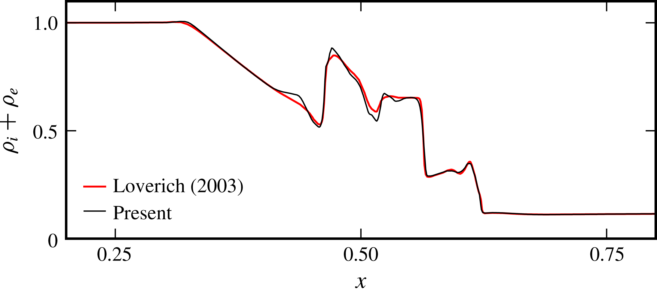
To compare with an existing solution of the two-fluid system of equations, the solution to an electromagnetic shock by Loverich (Reference Loverich2003) is used. In this test the plasma lengths are given as
 $d_{L}=1/300$
and
 $d_{D}=d_{L}/100$
with
 $c=100$
and
 $(m_{e}/m_{i})=(1/1836)$
. The simulation was run on a uniform one-dimensional grid of 1024 cells over a domain of
 $0\leqslant x\leqslant 1$
. The initial conditions for this test are
 $$\begin{eqnarray}\displaystyle \left(\begin{array}{@{}c@{}}\unicode[STIX]{x1D70C}_{i},\unicode[STIX]{x1D70C}_{e}\\ p\\ \boldsymbol{ u}\\ \boldsymbol{ B}\\ \boldsymbol{ E}\end{array}\right)=\left(\begin{array}{@{}c@{}}1,\displaystyle \frac{m_{e}}{m_{i}}\\ 0.5\\ \boldsymbol{ 0}\\ \left(\displaystyle \frac{3}{4},1,0\right)^{T}\\ \mathbf{0}\end{array}\right)_{x<(1/2)}=\left(\begin{array}{@{}c@{}}\displaystyle \frac{1}{8},\frac{1}{8}\frac{m_{e}}{m_{i}}\\ 0.05\\ \boldsymbol{ 0}\\ \left(\displaystyle \frac{3}{4},-1,0\right)^{T}\\ \mathbf{0}\end{array}\right)_{x\geqslant (1/2)}, & & \displaystyle\end{eqnarray}$$
where results are shown at
 $t=0.1$
in figure 4. In this figure the solution from the present solver is able to reproduce the solution by Loverich with the location and magnitude of all features in the combined density profile being captured. The present solver does appear to have lower numerical dissipation. This comparison gives confidence in the numerical method which is thus considered suitable for the following work.
Comparison of simulation results from the present solver to the numerical electromagnetic shock solution of Loverich (Reference Loverich2003).

4 Simulation initial conditions
Initial conditions for the RMI in
 $2$
-D
 $(x,y)$
space consist of a three-zone Riemann problem in the
 $y$
-periodic domain as shown in figure 1. Initial fields comprise three states denoted
 $(S_{0},S_{1},S_{2})$
separated by two interfaces. A left interface
 $I_{L}$
separating
 $S_{0},S_{1}$
is planar and defines the driving Riemann problem, while the right interface
 $I_{R}$
, separating
 $S_{1}$
and
 $S_{2}$
, is the perturbed density interface. Interface
 $I_{R}$
is defined to have a hyperbolic tangent density profile across the interface (aligned with
 $x$
) according to,
 $$\begin{eqnarray}\displaystyle f(x)=f_{R}+\frac{f_{L}-f_{R}}{2}\left(1+\tanh \left(\frac{2x}{\unicode[STIX]{x1D702}}\text{arctanh}\left[\frac{9f_{R}-10f_{L}}{10\left(f_{L}-f_{R}\right)}\right]\right)\right), & & \displaystyle\end{eqnarray}$$
where
 $f_{L}$
and
 $f_{R}$
give the left and right values and
 $\unicode[STIX]{x1D702}$
is the width containing 90 % of the variation. States are uniform with the ion initial conditions given by,
 $$\begin{eqnarray}\displaystyle \left(\begin{array}{@{}c@{}}\unicode[STIX]{x1D70C}\\ p\\ u_{x}\\ u_{y},u_{z}\end{array}\right)_{i,S_{0}}=\left(\begin{array}{@{}c@{}}2.286\\ 2.375\\ 1.027\\ 0\end{array}\right),\quad \left(\begin{array}{@{}c@{}}\unicode[STIX]{x1D70C}\\ p\\ \boldsymbol{u}\end{array}\right)_{i,S_{1}}=\left(\begin{array}{@{}c@{}}1\\ 0.5\\ \boldsymbol{ 0}\end{array}\right),\quad \left(\begin{array}{@{}c@{}}\unicode[STIX]{x1D70C}\\ p\\ \boldsymbol{u}\end{array}\right)_{i,S_{2}}=\left(\begin{array}{@{}c@{}}3\\ 0.5\\ \boldsymbol{ 0}\end{array}\right). & & \displaystyle\end{eqnarray}$$
The electron density is given by
 $\unicode[STIX]{x1D70C}_{e}=(m_{e}/m_{i})\unicode[STIX]{x1D70C}_{i}$
with all other quantities being identical to the ion species. State
 $S_{0}$
corresponds to the conditions downstream of a shock wave with hydrodynamic Mach number of
 $M_{s}=2$
in the ion species, matching the incident shock Mach number used in fundamental studies of the MHD RMI (Samtaney Reference Samtaney2003; Wheatley et al.
Reference Wheatley, Samtaney and Pullin2005, Reference Wheatley, Samtaney and Pullin2009, Reference Wheatley, Samtaney, Pullin and Gehre2014). The electron conditions are set relative to the ion conditions to maintain charge neutrality (
 $n_{e}=n_{i}$
), thermal equilibrium (
 $T_{e}=T_{i}$
) and velocity equilibrium (
 $\boldsymbol{u}_{e}=\boldsymbol{u}_{i}$
). The electron interface therefore defines a general Riemann problem since the sound speed of the electrons is significantly higher than that of the ions. Initial electromagnetic fields are
 $\boldsymbol{E}=0$
and
 $\boldsymbol{B}=0$
. Following other investigations using the two-fluid plasma model (e.g. Abgrall & Kumar (Reference Abgrall and Kumar2014)), the mass ratio between the species is set to 100 with
 $m_{i}=1$
and
 $m_{e}=0.01$
with
 $m_{0}=9.11\times 10^{-29}$
kg (100 times the dimensional electron mass). While still large, this mass ratio is lower than the physical value of 1836, and thus reduces the problem stiffness. The assigned charges are
 $q_{i}=1$
and
 $q_{e}=-1$
. As appropriate for a plasma,
 $\unicode[STIX]{x1D6FE}=(5/3)$
for both species. The density interface
 $I_{R}$
is sinusoidally perturbed with wavelength
 $1$
(the reference length scale
 $x_{0}$
is the dimensional perturbation wavelength) and amplitude
 $0.1$
, and has a density ratio
 $\unicode[STIX]{x1D70C}_{2}/\unicode[STIX]{x1D70C}_{1}=3$
where the transition is a tanh profile with scale length
 $0.01$
units.
 $I_{L}$
is positioned
 $0.2$
length units to the left of the mean of
 $I_{R}$
. The non-dimensional reference Larmor radius, Debye length and light speed are
 $d_{L}=d_{D}=0.1$
and
 $c=100.0$
, respectively, unless otherwise specified. Physically, this non-dimensional speed of light, which was also used by Loverich (Reference Loverich2003), implies a reference plasma temperature of
 $T_{0}=5.1\times 10^{3}$
eV, which is close to the hot-spot temperature in an ICF implosion (
 $T_{0}=5\times 10^{3}$
eV with
 $n_{0}=10^{31}$
(Srinivasan & Tang Reference Srinivasan and Tang2012)). While this temperature is at the upper limit of practical interest, this value of
 $c$
was chosen to make the problem more computationally tractable by lowering the range of wave speeds present. The reference number density depends on the values of
 $x_{0}$
and
 $d_{D}$
selected, as given by the equation for
 $n_{0}$
in § 2. Depending on the reference values chosen to dimensionalise the problem, the Debye lengths used presently, particularly
 $d_{D}=0.1$
, may result in kinetic effects being significant in the corresponding real plasma flow. We nonetheless utilise this relatively large Debye length to elucidate how two-fluid effects can alter Richtmyer–Meshkov flows, which is the purpose of the present study. The plasma length scales are subsequently reduced by an order of magnitude to investigate the flow closer to the single-fluid MHD limit, and it will become apparent that the
 $d_{D}=0.1$
case aids in understanding the results.
The simulations are run until
 $t=t_{final}=1.0$
. The above equations allow for the presence of external applied electric and magnetic fields that do not decay at infinity. These are not used presently and all fields are generated by charge separation.
The domain limits are
 $(-101\leqslant x\leqslant 101,0\leqslant y\leqslant 1)$
with periodic boundary conditions in
 $y$
and zero-gradient boundary conditions in
 $x$
. The length of the domain in
 $x$
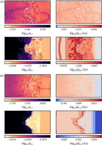
is determined by the speed of light and the location of the initial Riemann problem such that no electromagnetic waves may reach the non-periodic boundaries during the period of simulation. The AMR capability of the code is used to provide an effective resolution up to 4096 square cells per unit length with a base resolution of 8 cells and 7 levels of refinement (including the base grid) with factors of 4 for the first 3 levels and 2 for the remainder. Refinement of the grid is dictated by relative ion and electron density gradient,
 $$\begin{eqnarray}\frac{|\unicode[STIX]{x1D735}\unicode[STIX]{x1D70C}_{\unicode[STIX]{x1D6FC}}|\unicode[STIX]{x0394}x}{\unicode[STIX]{x1D70C}_{\unicode[STIX]{x1D6FC}}}>\frac{5}{100},\end{eqnarray}$$
as well as plasma length scale requirements where the smallest length scale is resolved by at least 2 cells. Note that refinement based on plasma length scales was only allowed where the normalised charge density exceeded the small threshold of
 $5/1000$
. The effectiveness of this AMR approach in adequately resolving the local plasma length scales in the present simulations is documented in appendix A.
Simulations in one dimension were carried out with the same initial conditions as the two-dimensional (2-D) case with geometric configuration corresponding to a zero amplitude density interface. These simulations were carried out on a uniform grid with results presented for a resolution of 2048 cells per unit length (unless otherwise specified).
4.1 Grid convergence
In the full two-dimensional numerical solutions presented subsequently, pointwise convergence is not expected as, in the absence of a physical dissipation mechanism, the vortex sheets present in the flow will continue to develop finer-scale structures as the grid is refined. There are, however, physical plasma length scales associated with high frequency oscillations that must be adequately resolved. These plasma oscillations occur in the one-dimensional (all quantities being functions of only
 $x$
and
 $t$
) base flow underlying the two-fluid RMI problem, thus their grid convergence can be studied without the confounding influence of vortex sheet roll up in this setting. To this end, the code base was used to simulate the one-dimensional base flow of the two-fluid RMI problem, equivalent to an initially flat interface, discretised with
 $N_{c}$
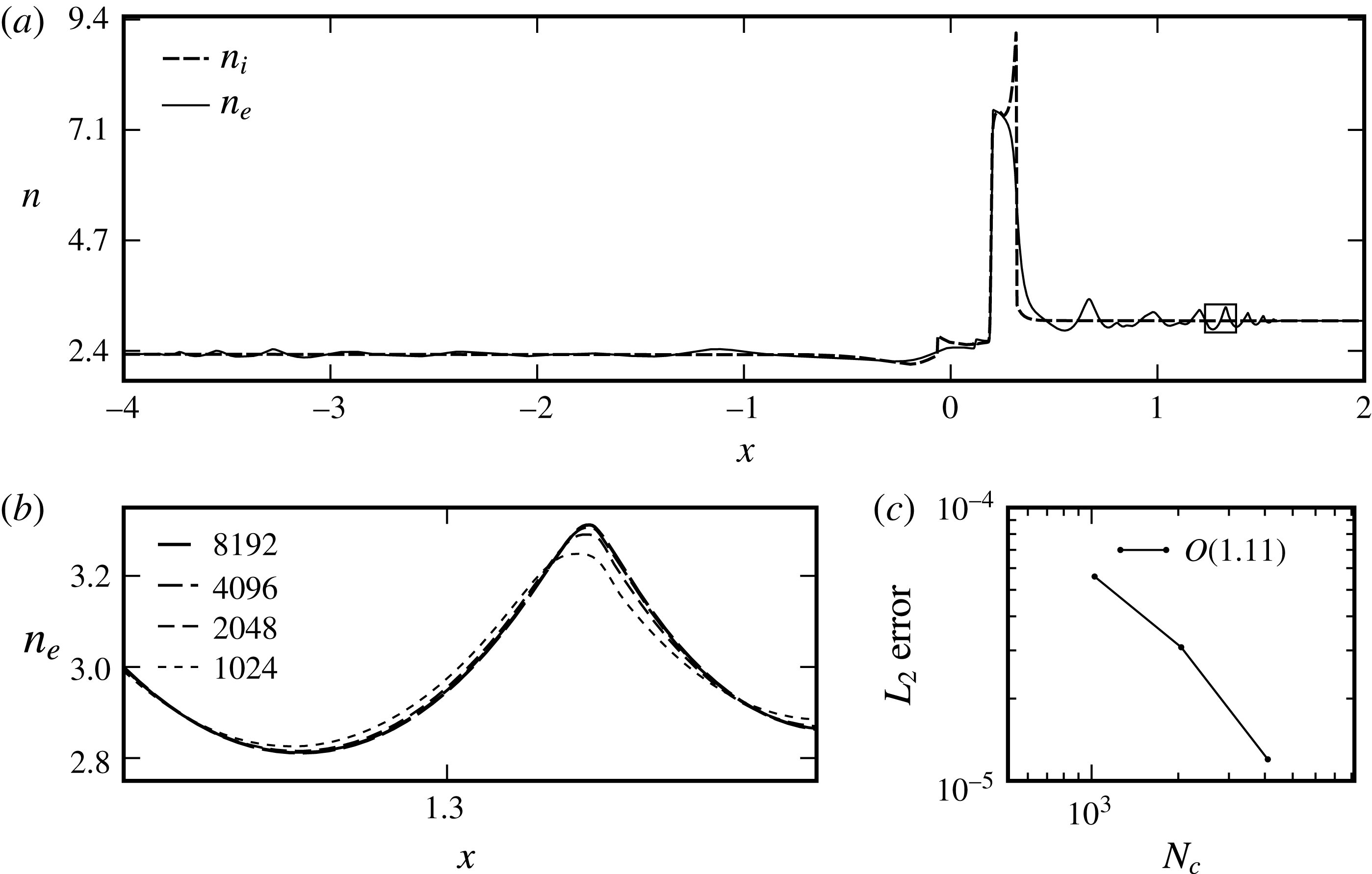
cells per unit length. Figure 5 shows the ion and electron density fields at
 $t=0.3$
for
 $N_{c}=1024,2048,4096,8192$
demonstrating grid convergence. The relatively low convergence rate of order 1.11 reported in this figure reflects the flow field being dominated by waves that activate the minmod limiter in the numerical implementation, causing the solver to locally revert to first-order accuracy. When the waves activating the limiter are widespread enough that the cumulative error in their vicinity dominates the global error norm, the global order of convergence can drop to near unity (Wheatley, Kumar & Huguenot Reference Wheatley, Kumar and Huguenot2010). From the expanded region displayed in figure 5 it may be seen that a resolution of
 $N_{C}=2048$
captures the essential details of the flow, with the mean
 $L_{2}$
-norm of the relative difference from the finest grid solution being equal to
 $5.6\times 10^{-5}$
. The minimum effective resolution adopted for the two-dimensional simulations is thus
 $N_{c}=2048$
.
(a) Ion and electron number density at a fixed time of
 $t=0.3$
from 1-D simulation, illustrating grid convergence. (b) Zoom in of detail showing
 $n_{e}$
with increasing
 $N_{c}$
. (c) Convergence rate with increasing
 $N_{c}$
in
 $L_{2}$
norm. Note presence of separate electron and ion shocks and plasma oscillations.

5 One-dimensional base flow
The wave structures that have been shown in figures 4 and 5 illustrate the complex flow fields that may be generated by the two-fluid plasma system. Thus before proceeding to investigate the RMI via two-dimensional simulations, we examine the features of the one-dimensional base flow that underlies it. The first point that may be investigated is the differing wave structures that are produced in the ion and electron fluids from the initial conditions. As stated in § 4, states
 $S_{0}$
and
 $S_{1}$
are defined to generate a Mach 2 shock in the ion fluid. The electron fluid interface, on the other hand, defines a general Riemann problem. This may be observed in figure 3 where, with electromagnetic interaction suppressed, the ion and electron Riemann problems produce a single normal shock, and a right propagating shock and a left propagating rarefaction, respectively.
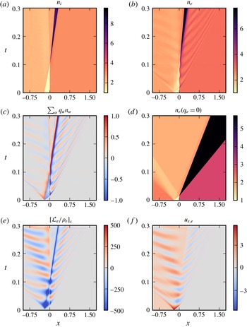
We next consider the wave structures produced in the full two-fluid case, with electromagnetic interactions appropriately enabled, which are visualised via the space–time evolution of the species number densities in figure 6(a,b). While the two-fluid effects acting on the ion fluid at early times are negligible owing to their greater mass, see figure 6(a), the effect on the electron fluid is significant. This may be seen when comparing the electron evolution, see figure 6(b), to an equivalent neutral fluid, see figure 6(d). From these figures, it is evident that the electromagnetic coupling to the ions significantly weakens the transmitted electron shock, causes substantial temporal oscillations of the electron density interface location, and generates widespread oscillatory waves on both sides of the interface. The acceleration producing the electron density interface oscillation is of particular interest due to its potential to drive RTI of the interface in the two-dimensional case. The mechanisms underlying the observed behaviour are revealed by considering the charge density produced by the relative motion of the ions and electrons (figure 6
c), the
 $x$
-acceleration of the electrons due to the Lorentz force
 ${\mathcal{L}}_{e}$
generated by the resultant electric field (figure 6
e), and the consequent electron
 $x$
-velocity evolution (figure 6
f).
Time and space diagrams showing evolution of the one-dimensional base flow underlying the two-fluid plasma RMI. (a) Ion number density. (b) Electron number density. (c) Charge density. (d) Neutral fluid number density (
 $m=m_{e}$
). (e) Lorentz acceleration of electrons in
 $x$
. (f) Electron velocity in
 $x$
.

Comparing figures 6(a) and 6(b), it is evident that the electron shock propagates more rapidly than the ion shock, owing to the ten times greater sound speed in the electron species. At early times, prior to
 $t\approx 0.02$
, the compression of the electron shock increases the downstream electron number density, while the co-located ions are approximately undisturbed. Consequently, figure 6(c) shows a large region of negative charge density downstream of the electron shock, and the balancing region of positive charge density downstream of the ion shock location. This widespread charge separation is augmented by the relative motion of the density interfaces after the impact of the electron shock: the high density electrons move to the right while the ions are near stationary, resulting in the intense narrow band of positive charge between the interfaces. The overall charge separation distribution causes an electric field to be generated that acts to pull the high density electrons back towards the ion shock, as indicated by the negative Lorentz acceleration shown in figure 6(e). Figure 6(f) shows that the acceleration is sufficiently strong that by
 $t\approx 0.03$
the electron velocity downstream of the shock has reversed directions, other than in a relatively thin region immediately downstream of the shock. Owing to the electrons high mobility the region of reversed electron velocity is widespread, extending across the density interface and beyond the ion shock location. Thus after having been initially accelerated forward by the electron shock, the induced electric field causes the electron density interface to subsequently reverse its direction of travel, constituting the first half-period of its oscillation. In addition, the depletion of electron momentum downstream of the transmitted shock causes it to weaken, eventually degenerating into the oscillatory wave packet shown in figure 5. Due to their high mobility and the lack of physical dissipation in the system, the left moving electrons are observed to ‘overshoot’, depleting the electron number density downstream of the electron shock below the ion number density, as can be seen by comparing figures 6(a) and 6(b) at
 $t\approx 0.03$
. This results in a region of positive charge density to the right of the electron interface, while the charge density to the left remains negative, as indicated in figure 6(c). Once the electron density interface overshoots the ion interface to the right, this is augmented by the intense narrow band of negative charge density seen at
 $t\approx 0.04$
. The electric field generated due to this charge distribution is shown in figure 6(e) to re-accelerate the electrons near the interface to the right, resulting in a positive interface velocity at
 $t\approx 0.05$
(see figure 6
f). Figure 6(a,f) shows that this oscillatory process continues, with gradually decreasing amplitude, until the end of the simulation time. The overall effect is a complex interplay between momentum, charge separation and the resulting electromagnetic field generation. We emphasise that while oscillations of the ion interface are not apparent in figure 6(a), the ions are subject to equal and opposite electromagnetic forces to the electrons, but their greater particle mass results in orders of magnitude lower accelerations. Thus once the interfaces are perturbed, both the electron and ion density interfaces could potentially be subject to electrically driven, variable acceleration RTI. Considering the ideal nature of the current simulations, the lack of physical dissipation mechanisms may cause the observed electromagnetic effects to be somewhat amplified relative to a real plasma flow.
6 RMI of a thermal interface
We now consider the planar RMI in a two-fluid plasma by applying a single-mode sinusoidal perturbation to the thermal interface in the one-dimensional base flow. To clearly elucidate the influence of two-fluid effects on the RMI, we first study a case where the reference plasma length scales are a significant fraction of the perturbation wavelength,
 $d_{L}=d_{D}=0.1$
, and thus these effects are expected to be significant. The evolution of the flow in this case is presented in § 6.1, followed by the generation of electromagnetic fields and the forces these apply to the fluids in § 6.2. In § 6.3, we subsequently examine a case with an order of magnitude smaller plasma length scales,
 $d_{L}=d_{D}=0.01$
, to investigate the behaviour of the flow closer to the single-fluid MHD limit. The resulting interface statistics for both cases are then presented in § 6.4.
6.1 Flow evolution
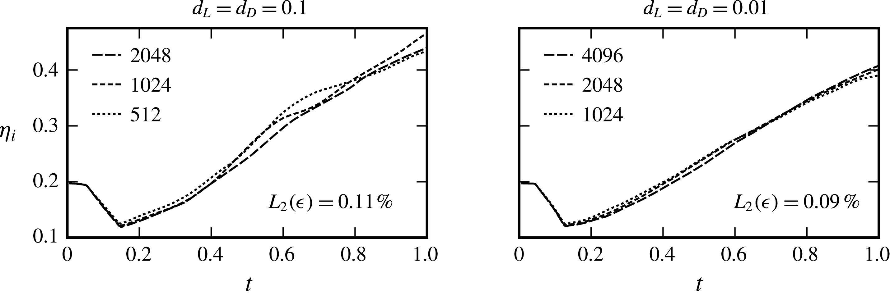
A square celled mesh with effective resolution of
 $2048$
cells per unit length was used for the 2-D simulation of the
 $d_{L}=d_{D}=0.1$
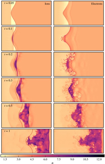
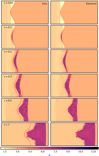
case. At this resolution, a grid convergence study (see appendix A) indicated that the interface width evolution is within 0.11 % of the Richardson extrapolated exact solution. The overall dynamics of the flow is illustrated in figure 7, which shows a time sequence of the ion and electron number density fields. A contour showing the evolution of the density interface in the single-fluid case, which was computed by the same solver on the same grid, is overlaid on the plots of
 $n_{i}$
. Comparing the interface behaviour between the single-fluid and two-fluid cases, it is apparent that two-fluid effects have given rise to a wealth of new flow physics. This has, amongst other things, resulted in a substantially greater interfacial growth rate compared to the single-fluid case and the occurrence of secondary instabilities.
Electron and ion flow evolution with
 $d_{L}=d_{D}=0.1$
in a stationary reference frame. These frames illustrate how the electron motion significantly distorts the ion shock. Hydrodynamic interface location is overlaid on ion plots.

Zoomed in contour plots of electron number density interface instabilities for
 $d_{L}=d_{D}=0.1$
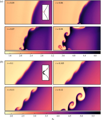
. The plot region is fixed in the laboratory reference frame and shown in the context of the full electron interface by the inset plot in first frame of each panel. (a) Electron Rayleigh–Taylor instability at the head of the spike at early time. The bulk motion of the interface is shown by comparison between these frames. (b) Electron Kelvin–Helmholtz instability at the transition between bubble and spike at intermediate time.

Due to their low inertia, the electron dynamics is much faster than that of the ions. It can be seen in figure 7 that the electron density interface grows more rapidly and develops secondary instabilities sooner. These gradually influence the high inertia ions though electromagnetic coupling. Understanding the evolution of the electron fluid is therefore critical to understanding the two-fluid plasma RMI. The electron density oscillations between the interface and the electron shock are apparent from early
 $t$
. As in the one-dimensional base flow, these oscillations result in a time-varying electromagnetic acceleration of the density interfaces which drive a secondary RTI.
The presence of the RTI is confirmed in § 6.4, where it will be shown that vorticity is baroclinically generated at the density interfaces continuously after the initial shock interaction, substantially increasing the growth of the first-mode interface perturbation. The electron RTI is first visible at high wavenumbers near the head of the spike (leftmost part of the interface). The RTI occurs in this region initially because it is the first part of the interface processed by the electron shock, and therefore the first to develop charge separation, an induced
 $x$
-electric field and consequent
 $x$
-acceleration. A close up of the interface development in this region is provided in figure 8(a). At
 $t=0.05$
, the first high wavenumber feature to significantly grow is only evident immediately adjacent to the domain centreline and has a wavenumber of
 $k_{y}\approx 220$
. The wavenumber of this feature was the same in a simulation with half the effective resolution carried out as part of the grid convergence study documented in appendix A. Note that although the interface was perturbed with a single mode, by
 $t=0.04$
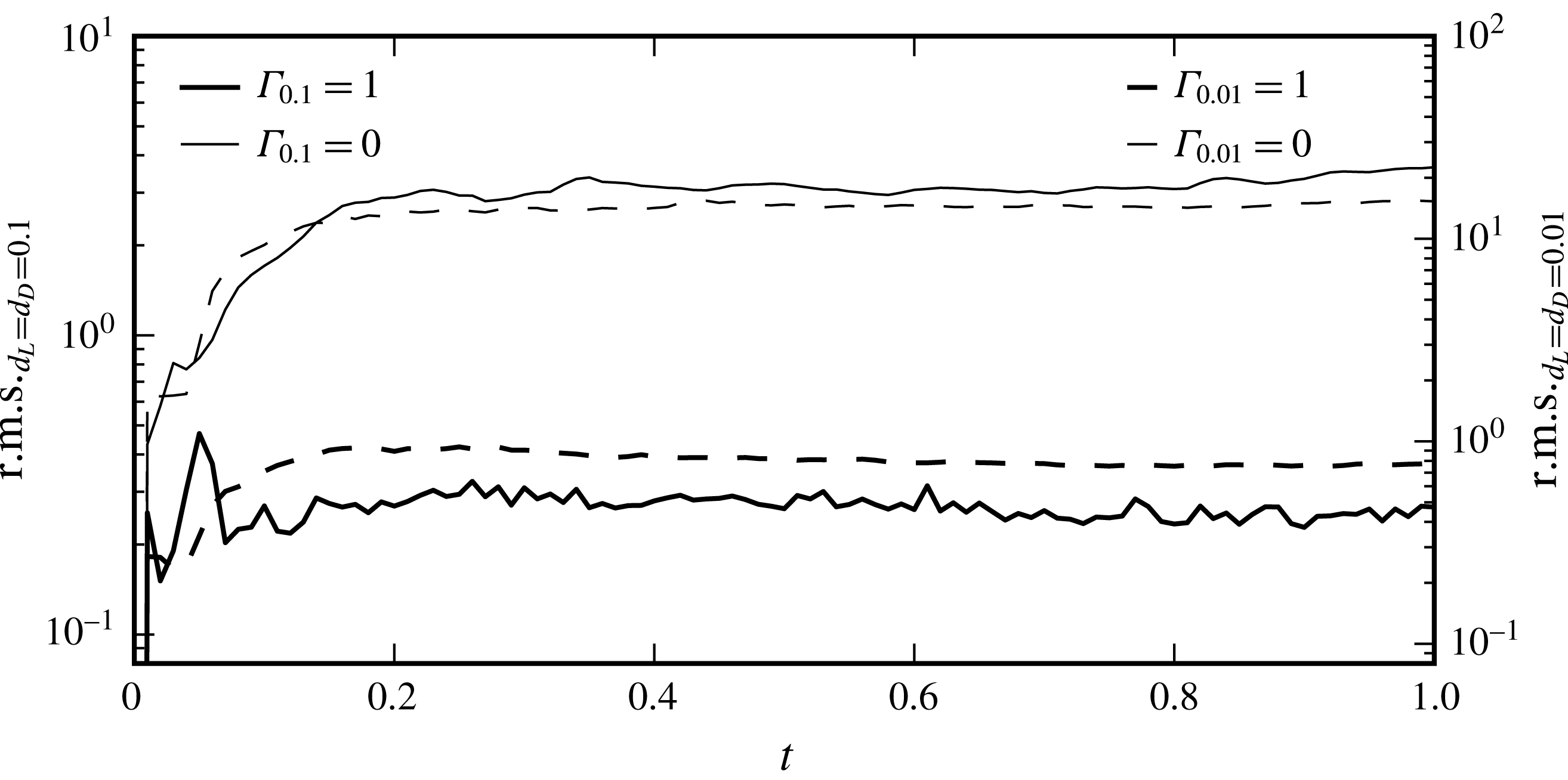
the vorticity deposited by the electron shock has distorted the interface to the extent that the spectrum of the interface perturbation has spread over a wide range of wavenumbers, as shown in figure 9. Thus all interface modes supported by the computational grid (
 $k_{y}<1024$
) are available for amplification.
By
 $t=0.06$
, figure 8(a) shows a more widespread lower wavenumber electron RTI mode growing on the head of the spike, with a wavenumber of
 $k_{y}\approx 50$
. As the bubbles and spikes associated with this mode grow, they interact with the primary-mode vorticity deposited on the interface by the electron shock. This scales with the slope of the interface in
 $y$
, and is thus zero at the centreline and edges of the domain. The primary-mode vorticity distribution both stretches the perturbations and, with increasing distance from the centreline (within the frame of figure 8
a), causes the evolution of the perturbations to increasingly become a combination of the RTI and the Kelvin–Helmholtz instability (KHI). By
 $t=0.08$
, the heads of the associated bubbles and spikes have rolled up into discrete vortices. The fine-scale flow features described above are regularised by numerical dissipation, and thus they are sensitive to the grid. As the grid is refined, in the absence of physical dissipation, the vortex sheets in this region will further roll up to generate even smaller scale flow features (Samtaney & Pullin Reference Samtaney and Pullin1996). The highly inclined portions of the electron interface, where the primary-mode vorticity from the RMI is strongest, begin to exhibit growth of a secondary KHI mode at a wavenumber of
 ${\approx}$
33 by
 $t=0.1$
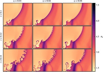
. A close up of the KHI development in one of these regions is shown in figure 8(b). In the grid convergence study documented in appendix A, we have verified that this most-amplified KHI mode has the same wavenumber on a grid with half the effective resolution. The most-amplified mode of the KHI is thus unlikely determined by the grid spacing in the present study. Increasing the interface thickness was also investigated (see appendix B) and was shown to delay the evolution of the KHI, but did not appear to significantly alter the wavenumber of the primary mode, at least within in the range of thicknesses investigated. By
 $t=0.12$
, this KHI mode has grown and rolled up into discrete vortices. Subsequently, the vortices generated by the RMI and secondary instabilities begin to interact, and by
 $t=0.2$
the electron flow field in the vicinity of the interface has become chaotic, thus flow symmetry is consequently broken.
Distribution of wavenumbers,
 $k$
, present in the electron interface at a time of
 $t=0.04$
, immediately after the electron shock transition. All of these modes are then present for amplification in the forthcoming electron instabilities.

At
 $t=0.2$
, figure 7 shows that the ion shock has just traversed the ion density interface, which still remains relatively smooth, in stark contrast to the chaotic electron interface at this time. While the time constant for the response of the heavier ion fluid to the forces induced by charge-density oscillations is much longer than for the electron fluid, by
 $t=0.5$
two notable effects are evident: First, the RTI of the ion interface is well developed at
 $t=0.5$
, causing substantially greater perturbation growth than in the single-fluid RMI case. The combined action of the RMI and secondary RTI have caused the development of the interface to enter the nonlinear regime in the two-fluid case. The high-wavenumber secondary instabilities present in the electrons are also evident in the ions, but take approximately an order of magnitude greater time to develop. Second, the ion shock, symmetrically perturbed by passage through the ion interface, is heavily distorted by the influence of the chaotic electron fluid. The ion shock does not simply pass through the electron field, the convection velocity of the electron vortices is sufficiently large that they are able to catch the ion shock from behind, pass through it and re-enter from upstream. Consequently, the ion shock encounters a temporally and spatially varying charge field that heavily perturbs the shock through the action of the resulting self-generated electromagnetic fields. The curvature of the perturbations to the ion shock surface then steepen, leading to the rapid formation of triple points. These shock–shock interactions generate reflected waves resulting in the cellular pattern in the ion density field behind the shock that is visible in the bottom left-hand panel of figure 7. At the same time the electron shock has degenerated almost completely into an oscillatory wave packet. This weakening is due to the effects of the electromagnetic fields as discussed in § 5. By
 $t=1$
the general structure and extent of the electron and ion density fields are similar, although the electron field has more small-scale content, indicating that approximate large-scale charge neutrality has been restored.
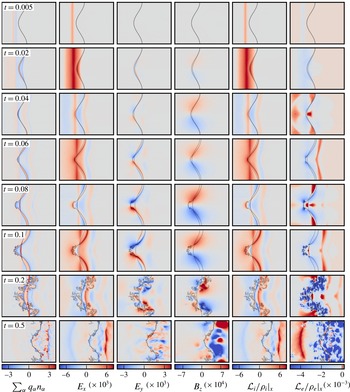
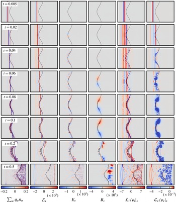
For the
 $d_{L}=d_{D}=0.1$
case, charge density, electric fields in
 $x$
and
 $y$
and magnetic field in
 $z$
. Acceleration in
 $x$
due to the Lorentz force acting on the ions (
 ${\mathcal{L}}_{i}$
) and electrons (
 ${\mathcal{L}}_{e}$
). Ion and electron interface locations shown for context. Note that the colour bar range has been truncated and centred on zero, the full range for each plot is
 $\sum _{\unicode[STIX]{x1D6FC}}q_{\unicode[STIX]{x1D6FC}}n_{\unicode[STIX]{x1D6FC}}=[-5.299,6.4642]$
,
 $E_{x}=[-0.0071,0.0089]$
,
 $E_{y}=[-0.0051,0.0053]$
,
 $B_{z}=[-0.0014,0.0014]$
,
 $({\mathcal{L}}_{i}/\unicode[STIX]{x1D70C}_{i})=[-6.6205,8.9296]$
,
 $({\mathcal{L}}_{e}/\unicode[STIX]{x1D70C}_{e})=[-8.798\times 10^{4},519.18]$
.

6.2 Field evolution
To illustrate the evolution of the electromagnetic fields, and their resulting action on the fluids, plots of the non-zero components of electric and magnetic fields are shown in figure 10, along with the
 $x$
-acceleration of the ions and electrons due to the Lorentz force (
 ${\mathcal{L}}_{\unicode[STIX]{x1D6FC}}/\unicode[STIX]{x1D70C}_{\unicode[STIX]{x1D6FC}}$
). The evolution of charge density is also shown to aid in understanding the electric field. The acceleration in
 $y$
is omitted in figure 10 as it is the
 $x$
-acceleration that is of primary interest due to the resulting RTI. For completeness, the acceleration in each direction due to the individual fields are shown in figure 11 for one particular instant,
 $t=0.04$
. All of the fields are entirely self-generated, according to (2.12) and (2.13).
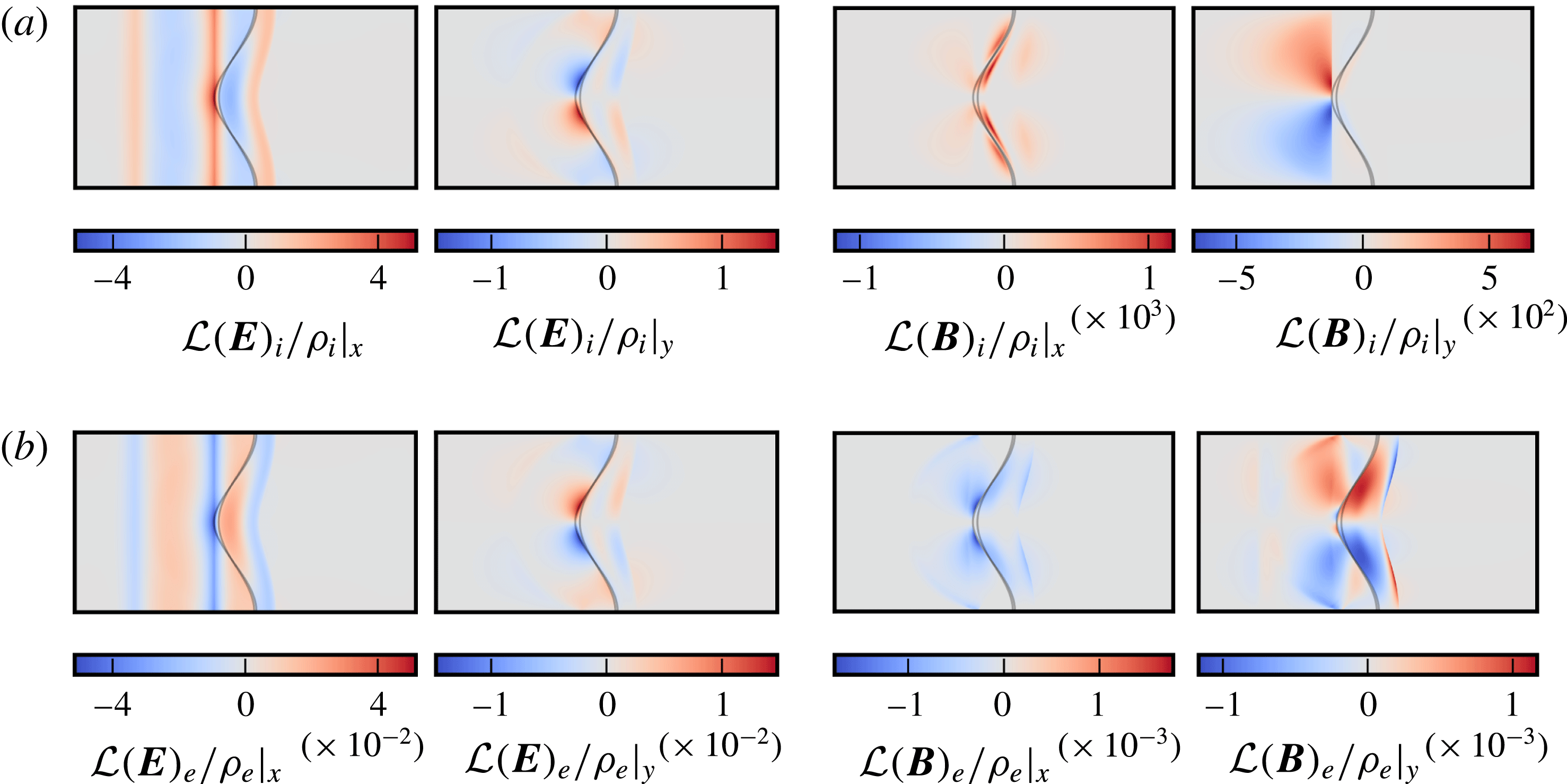
Accelerations of ions and electrons at
 $t=0.04$
due to the action of the electromagnetic fields in
 $x$
and
 $y$
. Ion and electron interface locations shown for context. (a) Ion accelerations in
 $x$
and
 $y$
at
 $t=0.04$
. (b) Electron accelerations in
 $x$
and
 $y$
at
 $t=0.04$
.

The nature of the initial conditions, Riemann problems that generate differing speed shocks in each species, encourages initial charge separation which immediately drives the generation of a strong electric field aligned with the fluid motion due to the resulting current density, as shown in (2.13). In general, the evolution of the charge density and the
 $x$
-electric field follows that in the one-dimensional case described in § 5, with added complexity due to the interface perturbation and subsequent instability. Following the initial charge density and electric field distributions established by differential shock and interface motion up to
 $t\approx 0.02$
, the highly mobile electron fluid is accelerated backwards by the field. Note that this acceleration initially occurs at the interface spike, since it is the first portion of the interface processed by the electron shock, and is in the Rayleigh–Taylor unstable direction, from heavy to light fluid. Due to the lack of dissipation in the system, the electrons overshoot the distribution that would neutralise the plasma, creating a deficit of negative charge downstream of the electron shock at
 $t=0.04$
, and an inversion of the sign of the electric field at the interface. From this point on, two main factors contribute to the charge-density distribution; the motion of plasma waves, which generate widespread net change, and the relative position of the electron and ion density interfaces, which creates a narrow band of net charge between them. The evolving charge distribution indicates that the process of overshooting electron fluid motion continues, causing oscillations in charge density and the sign of
 $E_{x}$
, which broadly results in an oscillatory
 $x$
-acceleration of the fluid in the vicinity of the interfaces.
At
 $t=0.2$
, the ion shock has just finished processing the ion density interface, and the transmitted shock has compressed a layer of high density ion fluid. This corresponds to the layer of net positive charge density to the right of the ion interface in the final row of figure 10. This positive layer is long lived compared to the negative layer formed downstream of the electron shock owing to the fact that the strength of the ion shock is not significantly abated during the simulation time, which in turn is a consequence of the slow ion dynamics. The presence of a long lived layer of net positive charge to the right of the ion interface results in
 $E_{x}$
becoming strongly negative at the ion interface. The consequent Lorentz acceleration of the ion interface is thus consistently negative for the remainder of the simulation, which is in the Rayleigh–Taylor unstable direction. It is interesting to note that despite the direction of the electric field, the electron interface is also subject to a negative
 $x$
-acceleration, which is therefore primarily caused by the influence of the magnetic field.
While the ion Lorentz
 $x$
-acceleration appears approximately equal to a scaled version of
 $E_{x}$
, the acceleration of the electrons is significantly modified by the magnetic field. This is illustrated in figure 11, which compares the accelerations of each fluid due to the electric and magnetic fields at
 $t=0.04$
. As expected, the species accelerations due to the electric field components differ by a factor of
 $-100$
, the product of the mass and charge ratios, since the particle acceleration scales with
 $q_{\unicode[STIX]{x1D6FC}}\boldsymbol{E}/m_{\unicode[STIX]{x1D6FC}}$
. The accelerations due to the magnetic field, however, are six orders of magnitude greater for the electrons. This is because in addition to the electrons having lower mass, the magnetic component of the Lorentz force is dependent on the fluid velocity, which is much greater for the electrons. For the ion fluid, the magnetic component of the Lorentz acceleration is three orders of magnitude smaller than the electric component and thus has little influence. For the electron fluid, on the other hand, the magnetic component peaks at the same order of magnitude as the electrical component and contributes significantly to the overall acceleration, particularly on the sides of the spike.
The coupled nature of the electric and magnetic field evolution can be observed when comparing
 $E_{y}$
and
 $B_{z}$
in figure 10. At
 $t=0.04$
, for example, differential charge motion parallel to the electron density interface, caused by the shock-induced vorticity on the electron interface while the ions are comparatively undisturbed, leads to generation of
 $\boldsymbol{E}$
parallel to the interface (with the primary component being
 $E_{y}$
) according to (2.13). Since the induced electron velocity due to the vorticity distribution decays away from the interface, so too does the current and the consequently generated
 $\boldsymbol{E}$
. Therefore this interface parallel
 $\boldsymbol{E}$
has an interface normal gradient, resulting in its curl being non-zero, which results in the generation of
 $B_{z}$
according to (2.13). This self-generated magnetic field is not aligned along a direction causing instability suppression in the MHD case (Wheatley et al.
Reference Wheatley, Samtaney and Pullin2005, Reference Wheatley, Samtaney, Pullin and Gehre2014). It should be noted that while this self-generated magnetic field does not have a major impact on the initially unmagnetised two-dimensional RMI considered here, the presence of such fields will become increasingly important in the magnetised and three-dimensional settings.
Ion and electron flow evolution with
 $d_{L}=d_{D}=0.01$
in a stationary reference frame. Hydrodynamic interface location overlaid on ion plots.

For the
 $d_{L}=d_{D}=0.01$
case, charge density, electric fields in
 $x$
and
 $y$
and magnetic field in
 $z$
. Acceleration in
 $x$
due to the Lorentz force acting on the ions (
 ${\mathcal{L}}_{i}$
) and electrons (
 ${\mathcal{L}}_{e}$
). Note that the colour bar range has been truncated and centred on zero, the full range for each plot is
 $\sum _{\unicode[STIX]{x1D6FC}}q_{\unicode[STIX]{x1D6FC}}n_{\unicode[STIX]{x1D6FC}}=[-2.7383,3.7094]$
,
 $E_{x}=[-0.0064,0.0083]$
,
 $E_{y}=[-0.0056,0.0060]$
,
 $B_{z}=[-0.0072,0.0068]$
,
 $({\mathcal{L}}_{i}/\unicode[STIX]{x1D70C}_{i})=[-62.435,117.98]$
,
 $({\mathcal{L}}_{e}/\unicode[STIX]{x1D70C}_{e})=[-7.604\times 10^{5},3.732\times 10^{3}]$
.

6.3 Reduced plasma length scale case
As
 $d_{L}$
and
 $d_{D}$
decrease, the single-fluid MHD quasi-neutral limit is approached (although it is only formally approached if electron inertia is also neglected). To investigate how the two-fluid plasma RMI of a thermal interface behaves closer to this limit, a case with reference
 $d_{L}=d_{D}=0.01$
was simulated with an effective resolution of
 $4096$
per unit length. At this resolution, a grid convergence study (see appendix A) indicated that the interface width evolution is within 0.09 % of the Richardson extrapolated exact solution. The evolution of
 $n_{i}$
and
 $n_{e}$
for this case is illustrated in figure 12. It is apparent that the electron and ion dynamics are much more strongly coupled in this case, with the result that the structure of the ion and electron density fields are very similar at each time shown. The primary difference occurs at
 $t=0.1$
, where the electrons develop small-scale structures on the spike that only weakly affect the ion density. The similarity of the number density distributions implies that the extent of charge separation is much smaller. This is verified in figure 13, which shows the electromagnetic fields and resulting accelerations for the
 $d_{L}=d_{D}=0.01$
case. As the extent over which charge separation occurs is reduced, consistent with the reduced reference Debye length, the induced electric and magnetic fields become more localised to the shock and interface locations. We emphasise that the electromagnetic effects seen in the larger plasma length scale place are still present, they just occur over smaller distances. Plots of
 $x$
-acceleration due to the Lorentz force confirm that the interfaces are subject to the same order of magnitude acceleration as in the previous case, which again drives the RTI. The influence of the electromagnetically driven RTI is thus reduced, however, leading to the perturbation growth exceeding that seen in the single-fluid case to a lesser extent than for
 $d_{D}=0.1$
, especially for the electrons. Overall, reducing the plasma length scales in the two-fluid case has caused the ion interface to develop high wavenumber content sooner, as a result of tighter coupling to the more unstable electron fluid, while the instability of the electron interface is restrained by the tighter coupling to the high inertia ion fluid.
In contrast to figure 10, the significantly more localised plasma features visualised in figure 13 generate more complex wave structures. This is particularly evident for
 $E_{x}$
where the initially uniform and diffuse field for the
 $d_{L}=d_{D}=0.1$
case is replaced by a highly oscillatory field at very early time. This complex wave structure interacts with the density interfaces at approximately the same time but results in reflected waves of reduced, but comparable, strength. This interaction leads to high wavenumber oscillations in both the
 $E_{x}$
and
 $E_{y}$
field leading to fine-scale acceleration and perturbation of the density interfaces at early time. The magnetic field,
 $B_{z}$
, maintains a diffuse nature as the reference plasma length scales decrease, albeit with increased magnitude. This increase in strength leads to greater influence on the flow, as seen in figure 15, and will be discussed later. At later times the chaotic nature of the flow around the interfaces leads to significant mixing in sign of the fields and accelerations leading to a reduction in the effect of concerted acceleration and the associated RTI.
6.4 Interface statistics
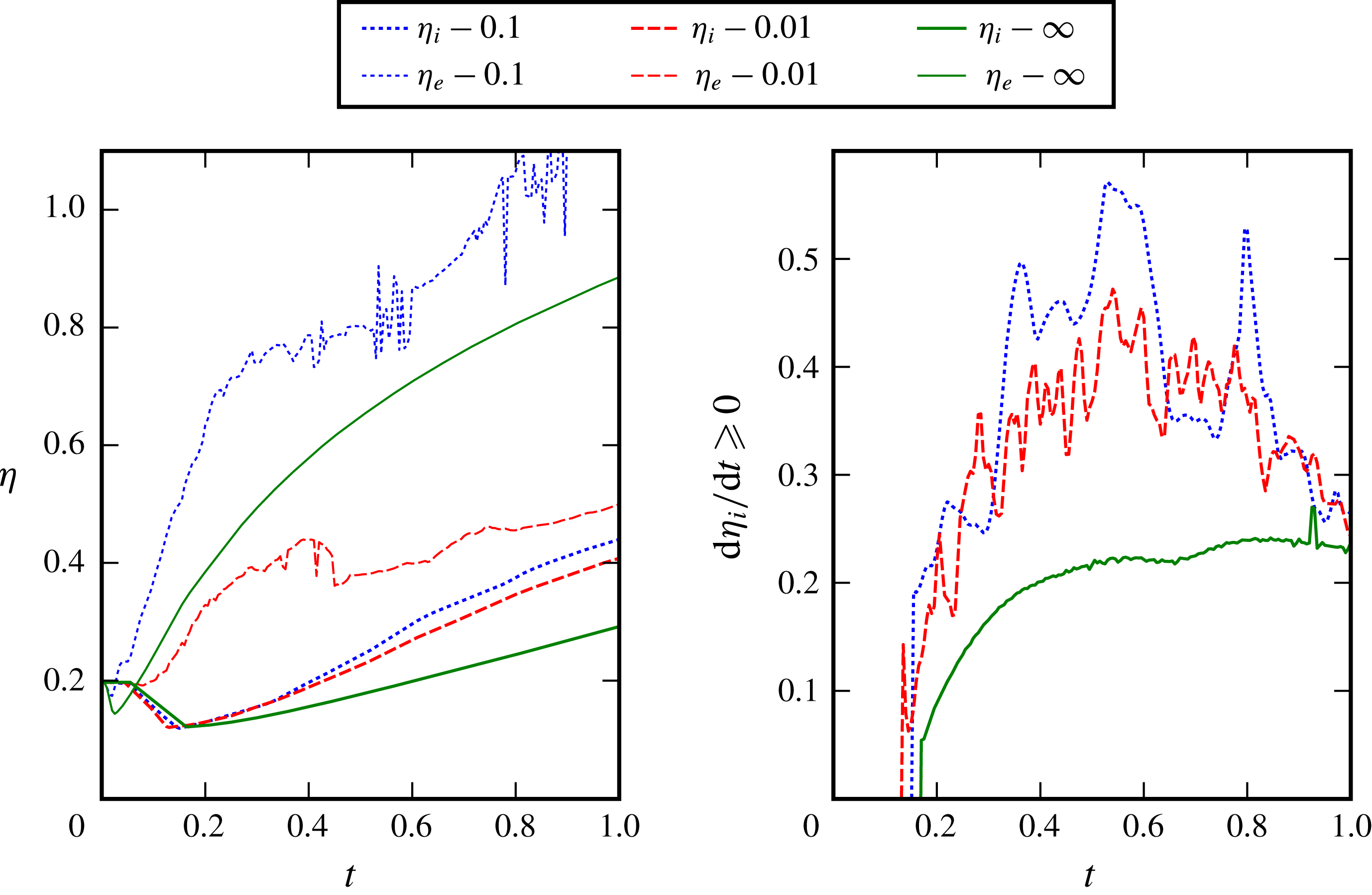
The extent in the
 $x$
-direction (referred to as the interface width,
 $\unicode[STIX]{x1D702}$
) of the density interfaces shown in figures 7–13, as well as for the hydrodynamic reference case, are shown over time in figure 14. The growth rates of the ion species interface widths are also shown. The extent of the interface in this case is defined as the region where
 $0.05\leqslant \unicode[STIX]{x1D71A}_{\unicode[STIX]{x1D6FC}}\leqslant 0.95$
, where
 $\unicode[STIX]{x1D71A}_{\unicode[STIX]{x1D6FC}}\in [0,1]$
is the volume-of-fluid tracer for each species. The interface width is calculated by reducing the data to a one-dimensional representation by integration across the domain, then determining the
 $x$
-locations where the values of
 $\unicode[STIX]{x1D71A}$
defining the interface occur.
Interface width and growth rate over time for the plasma conditions simulated. Numbers shown in the legend indicate the pertinent plasma length scale, where
 $\infty$
represents neutral species.

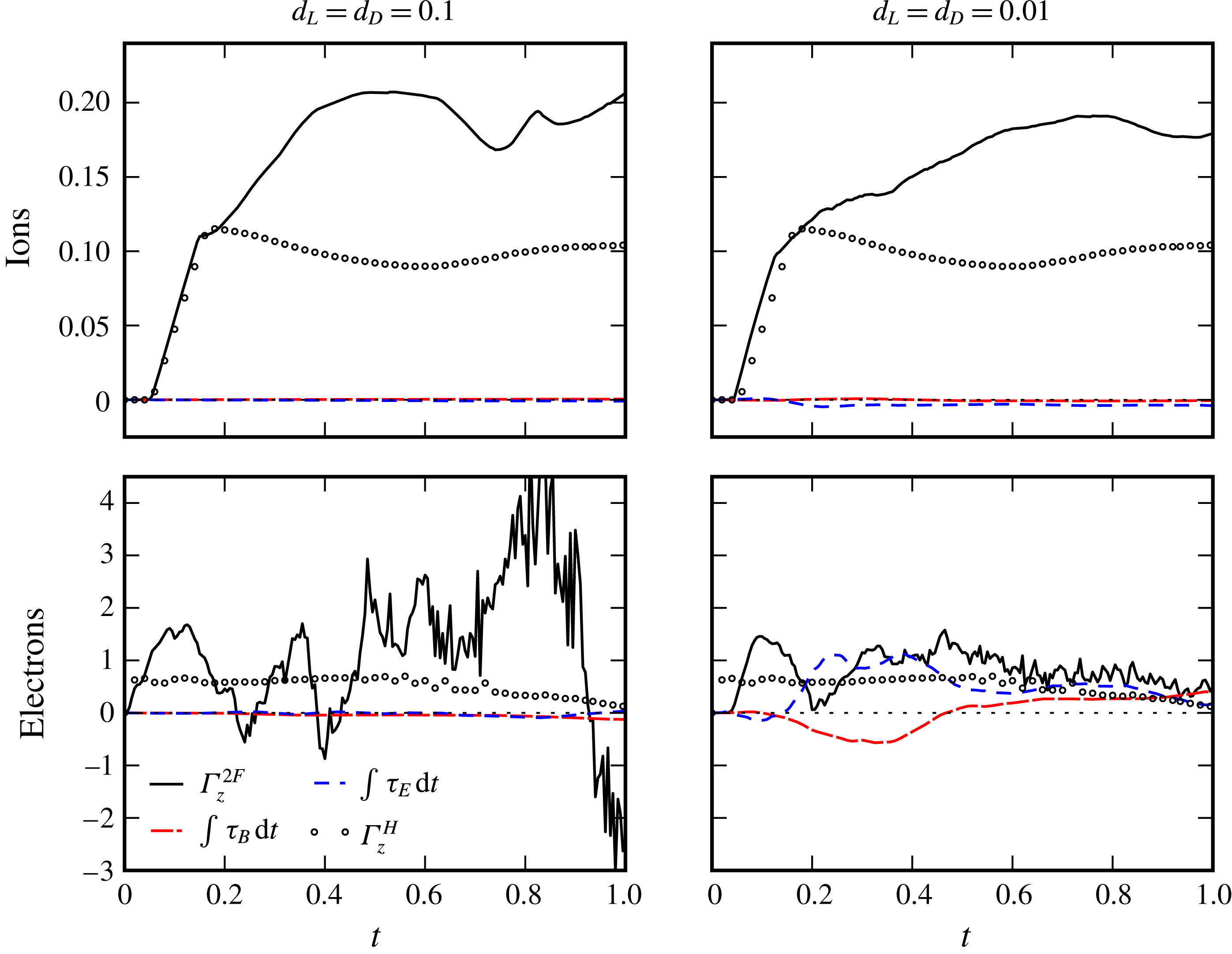
Ion and electron circulation (
 $\unicode[STIX]{x1D6E4}_{z}^{2F}$
) compared to the hydrodynamic equivalent (
 $\unicode[STIX]{x1D6E4}_{z}^{H}$
) along with cumulative time integral of Lorentz force magnetic (
 $\unicode[STIX]{x1D70F}_{B}$
) and electric (
 $\unicode[STIX]{x1D70F}_{E}$
) components over half of the domain (
 $y<0.5$
). Values computed on the interface of each species.

Since the ion species contains the vast majority of the fluid mass, it is the instability of the ion density interface that is of primary interest in most applications. In ICF, for example, the ion species is the fuel in which a fusion burn is to be ignited. Thus we primarily focus our attention on the ion interface statistics. The results presented in figure 14 show that, following the shock traversal and compression of the interfaces, the two-fluid interface width outpaces the reference hydrodynamic width in both magnitude and rate for all cases except electrons at small plasma reference length. For the
 $d_{L}=d_{D}=0.1$
and
 $d_{L}=d_{D}=0.01$
cases, the peak non-dimensional growth rates of the ion interface widths are 0.57 and 0.47, respectively, while the corresponding hydrodynamic growth rate is 0.24. Thus the instability of the interface is substantially amplified in the two-fluid case. Consequently, the ion interface widths at the final simulation time for the
 $d_{L}=d_{D}=0.1$
and
 $d_{L}=d_{D}=0.01$
cases are 2.2
 $\unicode[STIX]{x1D702}_{0}$
and 2.0
 $\unicode[STIX]{x1D702}_{0}$
, respectively, while the value for the hydrodynamic case is substantially lower at 1.5
 $\unicode[STIX]{x1D702}_{0}$
. For the two plasma regimes investigated, the growth rate of the ion interface returned to close to the hydrodynamic level by the end of the simulation, while the electron interface behaviour remained significantly different. When
 $d_{L}=d_{D}=0.1$
significant charge separation is allowed to occur due to the relatively large reference Debye length, this allows for the electron interface to grow more freely in response to its greater acceleration with less moderating influence from the inertia bound ions. For
 $d_{L}=d_{D}=0.01$
the ions and electrons are coupled much closer and so the electrons are effectively restrained by the more massive species leading to the significantly reduced interface growth relative to the alternative case.
In § 6, the occurrence of electromagnetically driven RTI in the two-fluid plasma RMI flow was discussed. The enhanced growth in the ion interface width was attributed to this. Here, we attempt to quantify the relative importance of the RMI and RTI by examining the source of the circulation present on the interfaces throughout the simulations. The ion and electron circulation on the lower half of the interface is computed by numerically integrating,
 $$\begin{eqnarray}\unicode[STIX]{x1D6E4}_{\unicode[STIX]{x1D6FC}}=\int _{0}^{0.5}\int _{a(y)}^{b(y)}\unicode[STIX]{x1D714}_{z,\unicode[STIX]{x1D6FC}}\,\text{d}x\,\text{d}y,\end{eqnarray}$$
where
 $\unicode[STIX]{x1D71A}_{\unicode[STIX]{x1D6FC}}(a(y),y)=0.01$
and
 $\unicode[STIX]{x1D71A}_{\unicode[STIX]{x1D6FC}}(b(y),y)=0.99$
. Once an interface becomes chaotic, such that vortices are convected between the upper and lower halves of the interface, this quantity ceases to be a useful measure of the sources of circulation. Fortunately, this does not occur significantly in the ion species in the cases under consideration until late in the simulation duration (
 $t>0.5$
). The histories of
 $\unicode[STIX]{x1D6E4}$
for the two-fluid and hydrodynamic simulations are shown in figure 15 along with the cumulative integral of the electric and magnetic components of the curl of Lorentz force (
 $\unicode[STIX]{x1D70F}_{E}$
,
 $\unicode[STIX]{x1D70F}_{B}$
) acting on each species interface, which generate vorticity according to (2.16). For both two-fluid cases, the ion circulation production is initially dominated by the deposition of vorticity on the interface by the traversing shock. This appears as an approximately linear increase in
 $\unicode[STIX]{x1D6E4}$
during the shock traverse, is responsible for the RMI and closely matches the hydrodynamic case. After the shock interaction is complete, the circulation on the two-fluid and hydrodynamic interfaces diverge, with continued generation of circulation in the two-fluid cases as opposed to gradual dissipation in the hydrodynamic case. In the
 $d_{D}=0.1$
case, the peak non-dimensional circulation (0.21 at
 $t=0.53$
) is close to double that in the hydrodynamic case (0.12 at
 $t=0.175$
), and is only slightly lower (0.19 at
 $t=0.76$
) in the
 $d_{D}=0.01$
case. The direct circulation generation due to electromagnetic forces on the ions, through the curl of Lorentz force, is found to be negligible for both cases. The influence is larger in the
 $d_{D}=0.01$
case and is due to the curl of
 $\boldsymbol{B}$
, and mildly opposes the growth of the interface. Thus the primary post-shock-interaction circulation generation is baroclinic in nature, as this is the only other source term in the vorticity equation, and results from the linear acceleration of the interface, as in the RTI. The
 $x$
-acceleration of the interface was demonstrated to be due to electromagnetic effects in § 6. The circulation generated in this electromagnetically driven RTI adds to that generated in the shock-interaction process and consequently increases the growth rate of the interface.
The circulation on the electron interface follows a similar pattern, at least initially, with a notable delay of the onset of circulation growth relative to the hydrodynamic case, especially for
 $d_{L}=d_{D}=0.01$
. This delay is due to the interaction with the ions in the two-fluid case, through the fields, slowing the electron shock relative to the hydrodynamic case. Following an initial increase, associated with the shock transition, there is a rapid rise beyond the hydrodynamic circulation level due to the initial backwards acceleration of the electron interface shown in § 6. Subsequently, the acceleration oscillates in sign until at least
 $t=0.2$
, which is reflected in the minor variations in circulation. Unfortunately, the electron interface becomes chaotic by
 $t=0.2$
for the
 $d_{L}=d_{D}=0.1$
case, and the circulation metric on the lower half of the interface becomes disrupted by vortices being convected in and out of the domain of integration. Thus the metric is not useful for the electron interface beyond this time. It is interesting to note that for the
 $d_{L}=d_{D}=0.01$
case, the curl of the Lorentz force has a significant influence on the electron interface circulation. The magnetic term initially generates circulation with sign opposing the baroclinically generated circulation, before augmenting it later in the interface development. The curl of the electric field, on the other hand, produces a substantial fraction of the circulation on the interface after
 $t=0.2$
.
7 Conclusions
In summary, the two-fluid plasma single-mode RMI of a thermal interface investigated here differs substantially from the hydrodynamic case. The Riemann problem used to initialise the flow drives a precursor electron shock that creates substantial charge separation. Following the passage of the electron shock through the perturbed interface, the electron density distribution continually overshoots that which would neutralise the plasma, resulting in an oscillatory electric field that causes oscillations of the density interfaces. This drives variable acceleration RTI of the interfaces. Consequently the electron interface, which is subject to orders of magnitude greater acceleration, rapidly develops fine-scale structures and becomes chaotic. The passage of the ion shock results in a longer lived region of net positive charge between the shock and the interface, resulting in sustained acceleration of the ion interface in the Rayleigh–Taylor unstable direction. The resulting RTI causes the growth of the low-mode ion interface perturbation to substantially exceed that seen in the single-fluid case. The transmitted ion shock is distorted and rapidly develops triple points due to its electromagnetic interaction with rapidly propagating electron vortices. These effects are reduced for a smaller Debye length plasma. The closer coupling between the ion and electron dynamics in that case does, however, result in the ion interface developing high wavenumber content earlier. Self-generated magnetic fields are observed in the vicinity of the shock-processed density interfaces, with the fields being more intense and localised for the smaller Debye length case.
The results of this fundamental study imply that shock-driven instabilities could potentially be more detrimental to ICF than predicted by single-fluid models: the increased interfacial growth rates and high wavenumber instability seen when two-fluid effects are accounted for may drive increased mixing, and the distortion of the transmitted ion shock may affect its convergence. The impact of the RMI in astrophysical settings may have been similarly underestimated. This should motivate future two-fluid studies, including collisional effects, at realistic plasma conditions appropriate to each application.
Acknowledgements
This research was supported by the KAUST Office of Sponsored Research under Award URF/1/2162-01. This work was supported by computational resources provided by the Australian Government under the National Computational Merit Allocation Scheme.
Appendix A. Results verification
Given the complexity of the physical system being simulated, various checks on the results generated may be carried out in order to increase confidence in those results. One important aspect of the simulation are the divergence constraints present in Maxwell’s equations, see (2.7) and (2.8), which are difficult to enforce in a discrete implementation. In this case the perfectly hyperbolic method (PHM) of Munz et al. (Reference Munz, Ommes and Schneider2000) is implemented according to (2.14) and (2.15). Simulations are then run with
 $\unicode[STIX]{x1D6E4}_{E}=\unicode[STIX]{x1D6E4}_{B}=0$
and
 $\unicode[STIX]{x1D6E4}_{E}=\unicode[STIX]{x1D6E4}_{B}=1$
to gauge the effect this method has on the steady state error present in the system. Due to the initial conditions and the two-dimensional nature of the simulation, there is no divergence present in the magnetic field, thus quantities for this measure will not be reported here. The root-mean-square (r.m.s.) error between divergence in the electric field and charge density is shown over time in figure 16 for the two cases simulated. From these results it can be observed that for both cases a reduction in r.m.s. error of approximately one order of magnitude is obtained when implementing PHM. It is, however, also of note that the system appears to sustain steady state error rates even with the divergence constraints turned off. This would suggest that while adding the divergence constraints is desirable it is not strictly necessary to perform stable simulations.
Time history of the discrete electric field divergence error (r.m.s.) for two plasma regimes (
 $d_{L}=d_{D}=0.1$
and
 $0.01$
) with the perfectly hyperbolic Maxwell divergence cleaning scheme.

The choice of
 $\unicode[STIX]{x1D6E4}=1$
in these simulations was dictated by the fact that
 $\unicode[STIX]{x1D6E4}$
gives the effective wave speed of the divergence cleaning process and as it acts as a multiplier of the speed of light,
 $c$
, can thus be the fastest wave speed in the system. While increasing
 $\unicode[STIX]{x1D6E4}$
over unity can increase the effectiveness of the divergence constraints, this introduces a decidedly non-physical aspect into the system where corrections to the flow field may occur ahead of any electromagnetic waves themselves. It is for this reason that
 $\unicode[STIX]{x1D6E4}$
was limited according to
 $\unicode[STIX]{x1D6E4}\leqslant 1$
.
Considering the large domain used for simulating these problems, see § 4, the choice of grid resolution becomes a significant practical consideration. For the plasma regimes simulated in this study the effective number of cells used is 2048 for
 $d_{L}=d_{D}=0.1$
and 4096 for
 $d_{L}=d_{D}=0.01$
. While pointwise convergence is difficult to obtain, given the complexity of the flow, it is possible to verify that integrated statistics of the flow are sufficiently converged. The interface width of the ions for the two cases simulated is thus calculated by simulations with varying effective resolutions and the Richardson extrapolated solution computed. The three solutions for ion interface width over time are shown in figure 17 for each plasma regime, along with the average
 $L_{2}$
norm calculated for the relative error of the fine grid solution to the Richardson extrapolated solution. Given that the calculated error in both cases is significantly below 1 % it is considered that the effective resolutions, of 2048 and 4096 cells per unit length for each case, are sufficient to capture the bulk flow characteristics of the interface evolution.
Time history of ion interface width for varying effective grid resolutions.

Larmor radius and Debye length (left) and ratio of Larmor radius and Debye length to cell size (right) at
 $t=0.75$
for electrons. Plasma length to cell size colour gradient centred at
 $(d/\unicode[STIX]{x0394}x)=2$
. Ion interface shown for spatial context. (a) Reference
 $d_{L}=d_{D}=0.1$
. (b) Reference
 $d_{L}=d_{D}=0.01$
.

According to the discussion in § 4, the adaptive mesh is refined to accommodate the plasma length scales such that wherever there is significant charge separation there is at least two cells per local Debye or Larmor length. This may be seen in figure 18 where the Larmor radius and Debye lengths, as well as the ratio with local cell size, are shown for the electron species. The electron species is discussed here due to the smaller length scales and thus the more stringent requirements on grid resolution. In this figure the plots of Larmor radius,
 $d_{L,e}$
, clearly indicate the presence of current loops in the plane with large continuous structures for larger reference plasma length scales and more numerous small-scale features in the case with smaller reference parameters. The local Debye length does not show such large-scale structures but is also significantly smaller in magnitude, it is therefore this length scale that dictates the choice of refinement. This may be seen in the right-hand column of figure 18 where the end result of the grid refinement strategy is evident. The ratio of plasma length to cell size is shown to be greater than 2 at all points downstream of the ion shock for both simulations, shown in figure 18(a,b), with regions upstream of the shock under-resolved for all but the Larmor radius with reference
 $d_{L}=d_{D}=0.1$
. This is a direct reflection of the AMR gridding strategy as there is minimal charge separation upstream of the ion shock and thus reduced need for the two-fluid effects to be fully resolved. From these results it is evident that the solutions are adequately resolved for the local plasma length scales involved.
Appendix B. Influence of initial interface thickness
The Kelvin–Helmholtz instability is known to be influenced by the initial thickness,
 $\unicode[STIX]{x1D702}$
, of the interface (Chandrasekhar Reference Chandrasekhar1961; Mishin & Morozov Reference Mishin and Morozov1983). In order to quantify this influence on the evolution of the electron KHI, shown for electrons in figure 8(b), a series of simulations were performed with
 $0.01\leqslant \unicode[STIX]{x1D702}\leqslant 0.04$
. Given the results presented until this point were with
 $\unicode[STIX]{x1D702}=0.01$
, these simulations investigate the effect of an interface with two and four times the initial thickness, and are shown in figure 19 over time. From these results it can be observed that increasing the interface thickness delays the evolution of the KHI but does not appear to significantly alter the wavenumber of the primary mode within the range of thickness investigated. The results presented in the main body of this work are thus considered a fair representation of the thermal interface RMI for the plasma parameters investigated.
The effect of increasing initial interface width on the evolution of the Kelvin–Helmholtz instability. Plots show electron number density contours of the upper half-domain at
 $0.1\leqslant t\leqslant 0.14$
and
 $d_{L}=d_{D}=0.1$
. Values of initial interface thickness
 $\unicode[STIX]{x1D702}$
as indicated.