2 Theoretical models and numerical approaches

As discussed above, here we approach the problem concerning the interaction of two Alfvénic wave packets by means of fluid and hybrid kinetic numerical simulations. For problems such as this, the system dimensionality is fundamental: in fact, a proper description should consider a three-dimensional physical space (i.e. three-dimensional wave vectors), where both parallel and perpendicular cascades are taken into account (Howes Reference Howes2015; Parashar et al. Reference Parashar, Matthaeus, Shay and Wan2015a , Reference Parashar, Oughton, Matthaeus and Wan2016). However, the dynamical range of the spatial scales (wavenumbers) represented in the model is equally important to capture nonlinear couplings during the wave packet interaction. Furthermore, performing a kinetic HVM simulation which contemporaneously includes a full three-dimensional 3D-3V phase space (three dimensions in physical space, three dimensions in velocity space) while also retaining a good spatial resolution is too demanding for the present high performance computing capability. Given that numerous runs are required to complete a study such as the present one, a fully 3D approach would be prohibitive. Therefore we adopt a 2.5D physical space, where vectorial fields are three-dimensional but their variations depend only on two spatial coordinates ( $x$ and $y$ ). It is worth noting that a 2.5D physical space captures the qualitative nature of many processes very well even though there might be some quantitative differences for some processes (Karimabadi et al. Reference Karimabadi, Roytershteyn, Daughton and Liu2013; Wan et al. Reference Wan, Matthaeus, Roytershteyn, Karimabadi, Parashar, Wu and Shay2015; Li et al. Reference Li, Howes, Klein and TenBarge2016).

The fluid models here considered are MHD and Hall MHD, whose dimensionless equations are:

In (2.1)–(2.4) spatial coordinates $\boldsymbol{x}=(x,y)$ and time $t$ are respectively normalized to $\tilde{L}$ and $\tilde{t}_{A}=\tilde{L}/\tilde{c}_{A}$ . The magnetic field $\boldsymbol{B}=\boldsymbol{B}_{0}+\boldsymbol{b}$ is scaled to the typical magnetic field $\tilde{B}$ , while mass density $\unicode[STIX]{x1D70C}$ , fluid velocity $\boldsymbol{u}$ , temperature $T$ and pressure $p=\unicode[STIX]{x1D70C}T$ are scaled to typical values $\tilde{\unicode[STIX]{x1D70C}}$ , $\tilde{c}_{A}=\tilde{B}/(4\unicode[STIX]{x03C0}\tilde{\unicode[STIX]{x1D70C}})^{1/2}$ , $\tilde{T}$ and $\tilde{p}=2\unicode[STIX]{x1D705}_{B}\tilde{\unicode[STIX]{x1D70C}}\tilde{T}/m_{p}$ ( $\unicode[STIX]{x1D705}_{B}$ being the Boltzmann constant and $m_{p}$ the proton mass), respectively. Moreover, $\tilde{\unicode[STIX]{x1D6FD}}=\tilde{p}/(\tilde{B}^{2}/8\unicode[STIX]{x03C0})$ is a typical value for the kinetic to magnetic pressure ratio; $\unicode[STIX]{x1D6FE}=5/3$ is the adiabatic index and $\tilde{\unicode[STIX]{x1D716}}=\tilde{d}_{p}/\tilde{L}$ (with $\tilde{d}_{p}=\tilde{c}_{A}/\tilde{\unicode[STIX]{x1D6FA}}_{cp}$ the proton skin depth) is the Hall parameter, which is set to zero in the pure MHD case. Details about the numerical algorithm can be found in Vásconez et al. (Reference Vásconez, Pucci, Valentini, Servidio, Matthaeus and Malara2015), Pucci et al. (Reference Pucci, Vásconez, Pezzi, Servidio, Valentini, Matthaeus and Malara2016).

On the other hand, hybrid Vlasov–Maxwell simulations have been performed by using two different numerical codes: the HVM code (Valentini et al. Reference Valentini, Travnicek, Califano, Hellinger and Mangeney2007) and a HPIC code (Parashar et al. Reference Parashar, Shay, Cassak and Matthaeus2009). For both cases, protons are described by a kinetic equation, while electrons are a Maxwellian, isothermal fluid. In the Vlasov model, an Eulerian representation of the Vlasov equation for protons is numerically integrated. In the HPIC method, the distribution function is Monte Carlo discretized and the Newton–Lorentz equations are updated for the ‘macro-particles’. Electromagnetic fields, charge density and current density are computed on a grid (Dawson Reference Dawson1983; Birdsall & Langdon Reference Birdsall and Langdon2004).

Dimensionless HVM equations are:

where $f=f(\boldsymbol{x},\boldsymbol{v},t)$ is the proton distribution function. In (2.5)–(2.7), velocities $\boldsymbol{v}$ are scaled to the Alfvén speed $\tilde{c}_{A}$ , while the proton number density $n=\int f\,\text{d}^{3}v$ , the proton bulk velocity $\boldsymbol{u}=n^{-1}\int \boldsymbol{v}f\,\text{d}^{3}v$ and the proton pressure tensor $\unicode[STIX]{x1D6F1}_{ij}=n^{-1}\int (v-u)_{i}\,(v-u)_{j}\,f\,\text{d}^{3}v$ , obtained as moments of the distribution function, are normalized to ${\tilde{n}}=\tilde{\unicode[STIX]{x1D70C}}/m_{p}$ , $\tilde{c}_{A}$ and $\tilde{p}$ , respectively. The electric field $\boldsymbol{E}$ , the current density $\boldsymbol{j}=\unicode[STIX]{x1D735}\times \boldsymbol{B}$ and the electron pressure $P_{e}$ are scaled to $\tilde{E}=(\tilde{c}_{A}\tilde{B})/c$ , $\tilde{j}=c\tilde{B}/(4\unicode[STIX]{x03C0}\tilde{L})$ and $\tilde{p}$ , respectively. Electron inertia effects have been considered in Ohm’s law to prevent numerical instabilities (where $m_{e}/m_{p}=0.01$ for $m_{e}$ the electron mass), while no external resistivity $\unicode[STIX]{x1D702}$ is introduced. A detailed description of the HVM algorithm can be found in Valentini et al. (Reference Valentini, Travnicek, Califano, Hellinger and Mangeney2007). On the other hand, the hybrid PIC run has been performed using the P3D hybrid code (Zeiler et al. Reference Zeiler, Biskamp, Drake, Rogers, Shay and Scholer2002) and all the numerical and physical parameters are the same as the HVM run. The code has been extensively used for reconnection and turbulence (e.g. Malakit et al. Reference Malakit, Cassak, Shay and Drake2009; Parashar et al. Reference Parashar, Shay, Cassak and Matthaeus2009).

In both classes of performed simulations (fluid and kinetic), the spatial domain $D(x,y)=[0,8\unicode[STIX]{x03C0}]\times [0,2\unicode[STIX]{x03C0}]$ is discretized with $(N_{x},N_{y})=(1024,256)$ in such a way that $\unicode[STIX]{x0394}x=\unicode[STIX]{x0394}y$ and spatial boundary conditions are periodic. For the HVM run, the velocity space is discretized with a uniform grid with $51$ points in each direction, in the region $v_{i}=[-v_{max},v_{max}]$ (with $v_{max}=2.5\tilde{c}_{A}$ ) and velocity domain boundary conditions assume $f=0$ for $|v_{i}|>v_{max}$ ( $i=x,y,z$ ). In the HPIC case, the number of particles per cell is $400$ . Moreover $\unicode[STIX]{x1D6FD}_{p}=2v_{th,p}^{2}/{\tilde{c}_{A}}^{2}=\tilde{\unicode[STIX]{x1D6FD}}/2=0.5$ (i.e. $v_{max}=5v_{th,p}$ ), $\boldsymbol{u}_{e}=\boldsymbol{u}-\tilde{\unicode[STIX]{x1D716}}\boldsymbol{j}/n$ , $\tilde{\unicode[STIX]{x1D716}}=9.8\times 10^{-2}$ , $k_{d_{p}}=\tilde{\unicode[STIX]{x1D716}}^{-1}\simeq 10$ and $k_{d_{e}}=\sqrt{m_{p}/m_{e}}\times \tilde{\unicode[STIX]{x1D716}}^{-1}\simeq 100$ . The background magnetic field is mainly perpendicular to the $x$ – $y$ plane: $\boldsymbol{B}_{0}=B_{0}(\sin \unicode[STIX]{x1D703},0,\cos \unicode[STIX]{x1D703})$ , where $\unicode[STIX]{x1D703}=\cos ^{-1}[(\boldsymbol{B}_{0}\boldsymbol{\cdot }\hat{\boldsymbol{z}})/B_{0}]=6^{\circ }$ and $B_{0}=|\boldsymbol{B}_{0}|$ .

In the initial conditions, ions are isotropic and homogeneous (Maxwellian velocity distribution function in each spatial point) for both kinetic simulations.

Large-amplitude magnetic $\boldsymbol{b}$ and bulk velocity $\boldsymbol{u}$ perturbations are introduced, while no density perturbations are taken into account (which implies non-zero total pressure fluctuations). Initial perturbations consist of two Alfvénic wave packets with opposite velocity–magnetic field correlation. The packets are separated along $x$ and, since $B_{0,x}\neq 0$ , they counter-propagate. The nominal time for the collision, evaluated with respect to the centre of each wave packet, is $\unicode[STIX]{x1D70F}\simeq 58.9$ .

The magnetic field perturbation $\boldsymbol{b}$ has been built in such a way that $\boldsymbol{B}_{0}\boldsymbol{\cdot }\boldsymbol{b}=0$ is satisfied in each spatial point. Then the velocity field perturbation $\boldsymbol{u}$ is built by imposing that $\boldsymbol{u}$ and $\boldsymbol{b}$ are correlated (anti-correlated) for the wave packet which moves against (along) $B_{0x}$ . A detailed discussion about the properties of the initial perturbations can be found in Paper I. The condition $B=|\boldsymbol{B}|=\text{const}$ is not satisfied by our initial perturbations, while this condition would be a requirement in defining a large-amplitude Alfvén mode in the context of a compressible MHD model. This suggests that pressure and density fluctuations are generated during the wave packet evolution.

The perturbation intensity is $\langle b\rangle _{rms}/B_{0}=0.2$ , therefore the Mach number is $M_{s}=\langle u\rangle _{rms}/v_{th,p}=0.4$ , where r.m.s. refers to the root mean square value. The intensity of fluctuations with respect to the in-plane field $B_{0x}$ is quite strong, with a value of approximately $2$ . This last parameter can be associated with $\unicode[STIX]{x1D70F}_{nl}/\unicode[STIX]{x1D70F}_{coll}$ (characteristic nonlinear time $\unicode[STIX]{x1D70F}_{nl}$ ; characteristic collision time $\unicode[STIX]{x1D70F}_{coll}$ ), whose value gives insight about the type of turbulence which could be generated. Here $\unicode[STIX]{x1D70F}_{nl}/\unicode[STIX]{x1D70F}_{coll}\simeq 0.5$ , hence nonlinear effects are important to approach a strong turbulence scenario.

3 Numerical results: a comparison between several codes

In this section we focus on the description of the results of the four different simulations (MHD, HMHD, HVM and HPIC) by focusing on some ‘fluid’-like diagnostics which help to understand the system dynamics and, also, to compare the numerical codes.

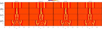
Figure 1 reports a direct comparison between the simulations, showing the contour plots of the out-of-plane component of the current density $j_{z}=(\unicode[STIX]{x1D735}\times \boldsymbol{B})\boldsymbol{\cdot }\hat{\boldsymbol{z}}$ . Vertical columns from left to right in figure 1 refer to MHD, HMHD, HVM and HPIC simulations, respectively; while each horizontal row refers to a different time instant: $t=29.5$ (a), $t=\unicode[STIX]{x1D70F}=58.9$ (b), $t=70.7$ (c) and $t=98.2$ (d).

Figure 1.

Contour plot of the out-of-plane component of the current density $j_{z}(x,y)$ at several time instants $t=29.5$ (a), $t=\unicode[STIX]{x1D70F}=58.9$ (b), $t=70.7$ (c) and $t=98.2$ (d). From left to right, each column refers to the MHD, HMHD, HVM and HPIC cases, respectively. For the HPIC simulation, $j_{z}(x,y)$ has been smoothed in order to remove particle noise.

Significant differences are recovered in the MHD case with respect to the HMHD, HVM and HPIC runs. While the MHD evolution is symmetric with respect to the centre of the $x$ direction, in the other cases this symmetry is broken also before the wave packets interaction due to the presence of dispersive effects which differentiate the propagation along and across the background magnetic field. Moreover, during the wave packets overlap (figure 1 b), smaller scale structures are formed in the HMHD and the HVM cases with respect to the pure MHD evolution, while the HPIC run – despite the fact that it recovers several significant features of the wave packets interaction – suffers from the presence of particle thermal noise, which has been artificially smoothed out in figure 1.

After the collision (figure 1 c,d), the difference between the MHD and the other simulations becomes stronger. In particular, some vortical structures at the centre of the spatial domain are recovered in the HMHD and HVM cases, in contrast to the pure MHD case. Moreover, the Vlasov simulation exhibits some secondary ripples in front of each wave packet whose nature could be related to some wave-like fluctuations. These secondary, low-amplitude ripples are not recovered in the other simulations: in fact, they cannot be appreciated in the HPIC run where the noise prevents the formation of such structures while in the Hall simulation they are only roughly visible. The nature of these low-amplitude ripples is compatible with a Kinetic Alfvén Waves activity and will be reported in detail in a separate paper.

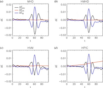
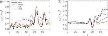
In order to compare models and codes, we display, in figure 2, the temporal evolution of the energy variations $\unicode[STIX]{x0394}E$ . Black, red and blue lines indicate respectively the kinetic $\unicode[STIX]{x0394}E_{kin}$ , thermal $\unicode[STIX]{x0394}E_{th}$ and magnetic $\unicode[STIX]{x0394}E_{B}$ energy variations, while each panel from (a) to (d) refers to the MHD, HMHD, HVM and HPIC runs, respectively. The evolution of $\unicode[STIX]{x0394}E_{kin}$ and $\unicode[STIX]{x0394}E_{B}$ is quite comparable in all the performed simulations and, in the temporal range where the wave packets collide, magnetic and kinetic energy is exchanged. On the other hand, the evolution of the thermal energy $\unicode[STIX]{x0394}E_{th}$ differs in the HPIC case compared to the other simulations. Indeed, $\unicode[STIX]{x0394}E_{th}$ remains quite close to zero for all the simulations except for the HPIC run, where it grows almost linearly due to the presence of numerical noise. It is worth to note that, as the number of particles increases, the evolution of $\unicode[STIX]{x0394}E_{th}$ becomes closer to the one obtained in the MHD, HMHD and HVM simulations.

Figure 2.

Temporal evolution of the energy terms: $\unicode[STIX]{x0394}E_{kin}$ (black), $\unicode[STIX]{x0394}E_{th}$ (red) and $\unicode[STIX]{x0394}E_{B}$ (blue) for the MHD, HMHD, HVM and HPIC runs.

Figure 3.

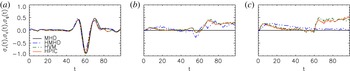
Temporal evolution of the normalized residual energy $\unicode[STIX]{x1D70E}_{r}(t)$ (a), cross-helicity $\unicode[STIX]{x1D70E}_{c}(t)$ (b) and generalized cross-helicity $\unicode[STIX]{x1D70E}_{g}(t)$ (c). In each panel black, blue, green and red lines indicate the MHD, HMHD, HVM and HPIC simulations, respectively.

The scenario described by Moffatt and Parker is also based on the property, in ideal incompressible MHD, that two wave packets separately conserve energy, which is equivalent to conservation of both total energy and cross-helicity $\unicode[STIX]{x1D70E}_{c}$ . It is natural therefore to examine evolution of cross-helicity as well as the evolution of the residual energy $\unicode[STIX]{x1D70E}_{r}$ , which gives information about the relative strength of magnetic fluctuations and the fluid velocity fluctuations. Figure 3(a,b) shows the temporal evolution of normalized residual energy $\unicode[STIX]{x1D70E}_{r}$ (a) and the normalized cross-helicity $\unicode[STIX]{x1D70E}_{c}$ (b). These quantities are defined as follows: $\unicode[STIX]{x1D70E}_{r}=(\text{e}^{u}-\text{e}^{b})/(\text{e}^{u}+\text{e}^{b})=2\text{e}^{u}/(\text{e}^{+}+\text{e}^{-})$ , where $\text{e}^{r}=\text{e}^{u}-\text{e}^{b}$ , $\text{e}^{\pm }=\langle (\boldsymbol{z}^{\pm })^{2}\rangle /2$ ( $\boldsymbol{z}^{\pm }=\boldsymbol{u}\pm \boldsymbol{b}$ ), $\text{e}^{u}=\langle \boldsymbol{u}^{2}\rangle /2$ and $\text{e}^{b}=\langle \boldsymbol{b}^{2}\rangle /2$ ; $\unicode[STIX]{x1D70E}_{c}=(\text{e}^{+}-\text{e}^{-})/(\text{e}^{+}+\text{e}^{-})=2\text{e}^{c}/(\text{e}^{u}+\text{e}^{b})$ , with $\text{e}^{c}=\langle \boldsymbol{u}\boldsymbol{\cdot }\boldsymbol{b}\rangle /2$ . In each panel of figure 3, black, dashed blue, dashed green and red lines refer to MHD, HMHD, HVM and HPIC cases, respectively.

Figure 3(a) shows the evolution of the normalized residual energy $\unicode[STIX]{x1D70E}_{r}$ , which is similar in all the simulations. In particular $\unicode[STIX]{x1D70E}_{r}\simeq 0$ in the initial stage, it oscillates when the wave packets overlap and finally it returns to $\unicode[STIX]{x1D70E}_{r}\simeq 0$ after the collisions. The $\unicode[STIX]{x1D70E}_{r}$ oscillations are well correlated with the oscillations of $\unicode[STIX]{x0394}E_{B}$ and $\unicode[STIX]{x0394}E_{kin}$ observed in figure 2.

Deeper insights are revealed by the evolution of the cross-helicity $\unicode[STIX]{x1D70E}_{c}$ . Indeed, for ideal incompressible MHD, the cross-helicity is conserved, and, for this initial condition, $\unicode[STIX]{x1D70E}_{c}=0$ . Here, $\unicode[STIX]{x1D70E}_{c}$ is well preserved in the MHD run despite this simulation being compressible. This means that the compressible effects, introduced here by the fact that initial perturbations are not pressured balanced, are not strong enough to break the $\unicode[STIX]{x1D70E}_{c}$ invariance. On the other hand, for the remaining simulations (HMHD, HVM and HPIC), $\unicode[STIX]{x1D70E}_{c}$ is not preserved: (i) it shows a jump around $t=\unicode[STIX]{x1D70F}=58.9$ , due to the presence of kinetic and dispersive effects, and (ii) there is an initial growth of $\unicode[STIX]{x1D70E}_{c}$ followed by a relaxation phase. It seems also significant to point out that the initial growth of $\unicode[STIX]{x1D70E}_{c}$ occurs faster in the kinetic cases compared to the HMHD one. This may reflect the fact that, the initial condition evolves differently in the Hall MHD simulation compared to the kinetic runs.

In order to understand the role of the Hall physics, we computed the normalized generalized cross-helicity $\unicode[STIX]{x1D70E}_{g}=2\text{e}^{g}/(\text{e}^{u}+\text{e}^{b})$ , where $\text{e}^{g}=0.5~\langle \boldsymbol{u}\boldsymbol{\cdot }\boldsymbol{b}+\tilde{\unicode[STIX]{x1D716}}\unicode[STIX]{x1D714}\boldsymbol{\cdot }\boldsymbol{u}/2\rangle$ and $\unicode[STIX]{x1D714}=\unicode[STIX]{x1D735}\times \boldsymbol{u}$ , which is an invariant of incompressible HMHD (Turner Reference Turner1986; Servidio, Matthaeus & Carbone Reference Servidio, Matthaeus and Carbone2008). Figure 3(c) displays the temporal evolution of $\unicode[STIX]{x1D70E}_{g}(t)$ for the MHD (black), the HMHD (dashed blue), HVM (dashed green) and HPIC (red) simulations. Note that the evolution of $\unicode[STIX]{x1D70E}_{g}$ is trivial for the MHD simulation since $\tilde{\unicode[STIX]{x1D716}}=0\;(\unicode[STIX]{x1D70E}_{g}=\unicode[STIX]{x1D70E}_{c})$ . Moreover, it can be easily appreciated that, for the HMHD case, $\unicode[STIX]{x1D70E}_{g}$ is almost preserved and does not exhibit any significant variation due to the collision itself, even though it shows a slight increase in the initial stages of the simulation followed by a decay towards $\unicode[STIX]{x1D70E}_{g}=0$ (similar to the growth of $\unicode[STIX]{x1D70E}_{c}$ recovered in figure 3 b). On the other hand, the two kinetic cases, which exhibit a similar behaviour, show a fast growth of $\unicode[STIX]{x1D70E}_{g}$ in the initial stage of the simulations followed by a decay phase (similar to the growth of $\unicode[STIX]{x1D70E}_{c}$ recovered in figure 3 b); then, during the collision, $\unicode[STIX]{x1D70E}_{g}$ significantly increases. We may explain the evolution of $\unicode[STIX]{x1D70E}_{c}$ and $\unicode[STIX]{x1D70E}_{g}$ as follows. In the MHD run, compressive effects contained in the initial condition as well as compressible activity generated during the evolution are not strong enough to break the invariance of $\unicode[STIX]{x1D70E}_{c}$ (i.e. of $\unicode[STIX]{x1D70E}_{g}$ ). Instead, in the Hall MHD simulation, the first break of the $\unicode[STIX]{x1D70E}_{c}$ invariance observed in the initial stage of the simulation cannot be associated with the Hall effect since also $\unicode[STIX]{x1D70E}_{g}$ is not preserved in this temporal region and $\unicode[STIX]{x1D70E}_{c}$ and $\unicode[STIX]{x1D70E}_{g}$ have a similar evolution. On the other hand, the jump recovered in $\unicode[STIX]{x1D70E}_{c}$ around $t\simeq \unicode[STIX]{x1D70F}=58.9$ is significantly related to the Hall physics. In fact, since $\unicode[STIX]{x1D70E}_{g}$ does not exhibit a similar jump at $t\simeq \unicode[STIX]{x1D70F}$ , we argue that the physics which produces the growth of $\unicode[STIX]{x1D70E}_{c}$ is the Hall physics (which is taken into account in the invariance of $\unicode[STIX]{x1D70E}_{g}$ ). Finally, the production of both $\unicode[STIX]{x1D70E}_{c}$ and $\unicode[STIX]{x1D70E}_{g}$ recovered in the kinetic simulations cannot be completely associated with the Hall effect (which, of course, is still present) but kinetic and compressive effects may have an important role.

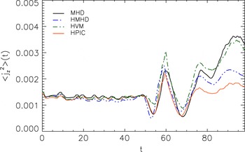
In order to explore the role of small scales in the dynamics of colliding wave packets, we computed the averaged mean squared current density $\langle j_{z}^{2}\rangle$ as a function of time. This quantity indicates the presence of small scale activity (such as production of small scale current sheets), and is reported in figure 4 for all the simulations. As in the previous figures, black, blue dashed, green dashed and red lines refer to the MHD, HMHD, HVM and HPIC cases, respectively. All models show a peak of $\langle j_{z}^{2}\rangle (t)$ around the collision time $t\simeq \unicode[STIX]{x1D70F}$ due to the collision of wave packets. After the collision, some high-intensity current activity persists in all the simulations, which present a qualitatively similar evolution of $\langle j_{z}^{2}\rangle (t)$ .

Figure 4.

Temporal evolution of $\langle j_{z}^{2}\rangle$ for the MHD (black), HMHD (blue), HVM (green) and HPIC (red) simulations. For the HPIC simulation $\langle j_{z}^{2}\rangle$ has been smoothed in order to remove particle noise.

Other quantities that provide physical details about our simulations are $\unicode[STIX]{x1D716}_{\unicode[STIX]{x1D70C}}=\langle \unicode[STIX]{x1D6FF}\unicode[STIX]{x1D70C}^{2}\rangle$ (compressibility) and the enstrophy $\unicode[STIX]{x1D716}_{\unicode[STIX]{x1D714}}=\langle \unicode[STIX]{x1D714}^{2}\rangle /2$ (fluid vorticity $\unicode[STIX]{x1D714}$ ). Note that $\unicode[STIX]{x1D6FF}\unicode[STIX]{x1D70C}=\unicode[STIX]{x1D70C}-\langle \unicode[STIX]{x1D70C}\rangle$ . Figure 5 reports the temporal evolution of $\unicode[STIX]{x1D716}_{\unicode[STIX]{x1D70C}}$ (a) and $\unicode[STIX]{x1D716}_{\unicode[STIX]{x1D714}}$ (b) for all the runs. Black, blue dashed, green dashed and red lines indicate respectively the MHD, HMHD, HVM and HPIC cases. The $\unicode[STIX]{x1D716}_{\unicode[STIX]{x1D70C}}$ evolution shows that density fluctuations peak around $t\simeq 63.8$ and $t\simeq 83.4$ . The two peaks are respectively associated with the collision between the packets and with the propagation of magnetosonic fluctuations generated by the initial strong collision which provide a sort of ‘echo’ of the original interaction. Moreover, from the initial stage of the simulations, $\unicode[STIX]{x1D716}_{\unicode[STIX]{x1D70C}}$ exhibits some modulations, which are produced by the absence of a pressure balance in the initial condition. In fact, as packets start to evolve, low-amplitude fast perturbations (clearly visible in the density contour plots, not shown here) propagate across the box and collide faster compared to the ‘main’ wave packets themselves. Moreover, by comparing the different simulations, one notices that, for $t\lesssim 20$ , kinetic and Hall runs tend to produce a similar evolution of $\unicode[STIX]{x1D716}_{\unicode[STIX]{x1D70C}}$ , slightly bigger compared to the MHD case. Then, around $t\simeq 20$ , the HMHD run displays a stronger compressibility with respect to the kinetic cases. This difference is probably due to the presence of kinetic damping phenomena which occur in the kinetic cases.

Figure 5.

Temporal evolution of $\unicode[STIX]{x1D716}_{\unicode[STIX]{x1D70C}}(t)$ (a) and $\unicode[STIX]{x1D716}_{\unicode[STIX]{x1D714}}(t)$ (b). In each panel black, blue, green and red lines indicate the MHD, HMHD, HVM and HPIC simulations, respectively. For the HPIC simulation, $\unicode[STIX]{x1D716}_{\unicode[STIX]{x1D714}}(t)$ has been smoothed in order to remove particle noise.

Figure 6.

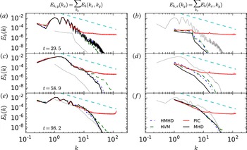
Magnetic energy power spectral densities $E_{b,y}(k_{x})=\sum _{k_{y}}E_{b}(k_{x},k_{y})$ (a,c,e) and $E_{b,x}(k_{y})=\sum _{k_{x}}E_{b}(k_{x},k_{y})$ (b,d,f) at three time instants: $t=29.5$ (a,b), $t=\unicode[STIX]{x1D70F}=58.9$ (c,d) and $t=98.2$ (e,f). In each panel black, blue, green and red lines refer to the MHD, HMHD, HVM and HPIC simulations, respectively, while cyan lines show the $-5/3$ slope for reference. Moreover, to compare $E_{b,y}(k_{x})$ and $E_{b,x}(k_{y})$ , the grey lines in each panel refer only to the MHD simulation and report $E_{b,x}(k_{y})$ (a,c,e) and $E_{b,y}(k_{x})$ in (b,d,f).

The enstrophy $\unicode[STIX]{x1D716}_{\unicode[STIX]{x1D714}}$ is displayed in figure 5(b). All the runs exhibit a similar evolution of $\unicode[STIX]{x1D716}_{\unicode[STIX]{x1D714}}$ up to the wave packets collision. Then MHD and HMHD cases exhibit a quite similar level of $\unicode[STIX]{x1D716}_{\unicode[STIX]{x1D714}}$ , slightly bigger compared to the one recovered in the HVM and HPIC cases, where probably kinetic damping does not allow the formation of strong vortical structures at small scales.

It is interesting to compare different simulations also by looking at power spectral densities (PSDs). Figure 6 show the magnetic energy PSD integrated along $k_{y}$ $E_{b,y}(k_{x})=\sum _{k_{y}}E_{b}(k_{x},k_{y})$ (a,c,e) and along $k_{x}$ $E_{b,x}(k_{y})=\sum _{k_{x}}E_{b}(k_{x},k_{y})$ (b,d,f); while each row respectively refers to $t=29.5$ (a,b), $t=\unicode[STIX]{x1D70F}=58.9$ (c,d) and $t=98.2$ (e,f). The cyan dashed line shows the $k^{-5/3}$ slope for reference while in each panel, black, blue, dashed green and red lines indicate respectively MHD, HMHD, HVM and HPIC simulations. Moreover, to compare the two wavenumber directions, grey lines in each panel report the corresponding PSD obtained from the MHD run, reduced in the other direction (for example, in figure 6(a), the grey line refers to $E_{b,x}(k_{y})$ for the MHD simulation while other curves in the same panel report $E_{b,y}(k_{x})$ ). It is interesting to note that, at $t=29.5$ , all the simulations exhibit a steep spectrum in $E_{b,y}(k_{x})$ , related to the initial condition, while the difference in power between $E_{b,y}(k_{x})$ and $E_{b,x}(k_{y})$ – the latter being significantly smaller than the former – tends to reduce in the final stages of the simulations. This suggests, as described in Paper I, the presence of nonlinear couplings which cause spectra to become more isotropic. Moreover the comparison between the different simulations indicates that the dynamics at large scales is described in a quite similar way for all runs, while at small scales, some differences are revealed. In particular, the HPIC simulation is affected by particle noise while the HVM run contains more energy at small scales compared to MHD and HMHD. Note that the presence, in MHD and HMHD runs, of an explicit resistivity prevents the population of small scales.

To summarize this section, we compared our numerical codes by analysing some global diagnostics and we conclude that the Moffatt–Parker scenario is quite well satisfied by MHD. However, other intriguing characteristics are observed when one moves beyond the MHD treatment. Moreover, the comparison between kinetic codes suggests that HVM and HPIC simulations display qualitatively similar features at large scales. However, when one aims to analyse the dynamics at small scales, HPIC simulations suffer from thermal particle noise. Magnetic energy spectra differ in the HPIC case compared with the HVM case. Moreover, by comparing the $j_{z}$ contour plots, one can easily appreciate how the HPIC simulation is affected by particle noise. Based on these considerations, we continue the analysis of the kinetic features produced in Alfvén wave packets collision by focusing only on the HVM case.

4 Kinetic features recovered during the wave packets interaction

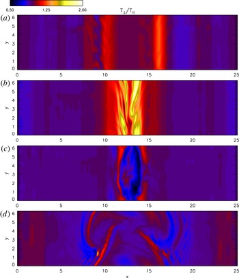
We begin a description of the kinetic signatures present in the Vlasov simulation by looking at the temperature anisotropy. Figure 7 reports the contour plots of the temperature anisotropy $T_{\bot }/T_{\Vert }$ , where the parallel and perpendicular directions are evaluated in the local magnetic field frame (LBF), at four time instants: $t=29.5$ (a), $t=\unicode[STIX]{x1D70F}=58.9$ (b), $t=70.7$ (c) and $t=98.2$ (d). Clearly, temperature anisotropy is present even before the main wave packets collide, due to the fact that the initial wave packets are not linear eigenmodes of the Vlasov equation and, hence, their dynamical evolution leads to anisotropy production. Moreover, a more careful analysis suggests that the left wave packet tends to produce regions where $T_{\bot }/T_{\Vert }<1$ close to the packet itself (which, as can be appreciated in figure 1, is localized around $x\simeq 9.5$ ), while the right wave packet (localized around $x=15.7$ ) is characterized by $T_{\bot }/T_{\Vert }>1$ . The presence of different temperature anisotropies is related to the broken symmetry with respect to the centre of the $x$ direction. Indeed, the dynamics of the wave packets is different if they move parallel or anti-parallel to $B_{0,x}$ . This produces the different temperature anisotropy recovered in figure 7(a).

Figure 7.

Contour plots of the temperature anisotropy for the HVM run evaluated in the local magnetic field frame (LBF) at four time instants: (a) $t=29.5$ , (b) $t=\unicode[STIX]{x1D70F}=58.9$ , (c) $t=70.7$ and (d) $t=98.2$ .

When the packets collide (figure 7 b), sheets characterized by a strong temperature anisotropy ( $T_{\bot }/T_{\Vert }>1$ ) are recovered, correlated spatially with the current density structures. Then, at $t=70.7$ (figure 7 c), wave packets split again and a region, localized at $(x,y)\simeq (14.3,1.0)$ , where the temperature anisotropy suddenly moves from values $T_{\bot }/T_{\Vert }<1$ towards $T_{\bot }/T_{\Vert }>1$ ones, is present. We will show that this region also shows the presence of strong departures from the equilibrium Maxwellian shape. At the final stage of the simulations (figure 7 d), each wave packet continues travelling, accompanied by a persistent level of temperature anisotropy, which is, indeed, well correlated with the current structures.

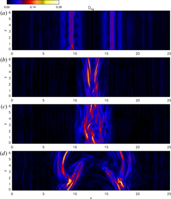
It is interesting to point out that, beyond the presence of temperature anisotropies, regions characterized by a non-gyrotropy are also recovered. Many methods have been proposed by evaluating the non-gyrotropy (Aunai, Hesse & Kuznetsova Reference Aunai, Hesse and Kuznetsova2013; Swisdak Reference Swisdak2016). Here we adopt the measure $D_{ng}$ (Aunai et al. Reference Aunai, Hesse and Kuznetsova2013), which is proportional to the root-mean-square of the off-diagonal elements of the pressure tensor. Figure 8 shows the contour plots of $D_{ng}$ at four time instants: $t=29.5$ (a), $t=\unicode[STIX]{x1D70F}=58.9$ (b), $t=70.7$ (c) and $t=98.2$ (d). Moreover, for the temperature anisotropy, the evolution of the two wave packets tends to produce non-gyrotropies also before the wave packets collision (figure 8 a). Then, during the collision (figure 8 b,c), the non-gyrotropy becomes more intense and it is also quite well correlated with the current structures. At the final stage of the simulation (figure 8 d), each wave packet is characterized by a level of non-gyrotropy which is quite bigger compared to the value before the collision. The presence of non-gyrotropic regions suggests that it is fundamental to retain a full velocity space where the VDF is let free to evolve and, eventually, distort.

Figure 8.

Contour plots of the degree of non-gyrotropy $D_{ng}$ , for the HVM run, evaluated in the LBF at four time instants: (a) $t=29.5$ , (b) $t=\unicode[STIX]{x1D70F}=58.9$ , (c) $t=70.7$ and (d) $t=98.2$ .

To further support the idea that kinetic effects are produced during the interaction of the wave packets, we computed the $L^{2}$ norm difference (Greco et al. Reference Greco, Valentini, Servidio and Matthaeus2012; Servidio et al. Reference Servidio, Valentini, Califano and Veltri2012, Reference Servidio, Valentini, Perrone, Greco, Califano, Matthaeus and Veltri2015):

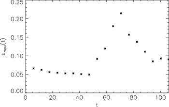
which measures the displacements of the proton VDF $f(\boldsymbol{x},\boldsymbol{v},t)$ with respect to the associated Maxwellian distribution function $f_{M}(\boldsymbol{x},\boldsymbol{v},t)$ , built such that density, bulk speed and total temperature of the two VDFs are the same. Figure 9 reports the evolution of the $\unicode[STIX]{x1D716}_{max}(t)=\max _{(x,y)}\unicode[STIX]{x1D716}(x,y,t)$ as a function of time. Clearly, as for the previous proxies of kinetic effects, also $\unicode[STIX]{x1D716}_{max}$ moves away from zero in the early phases of the simulation due to the fact that the initial condition is not a Vlasov eigenmode. Moreover, after the first initial variation, $\unicode[STIX]{x1D716}_{max}$ is almost constant until wave packets interact. Then, during the collision, $\unicode[STIX]{x1D716}_{max}$ grows and reaches its maximum at $t=70.7$ , later than the wave packets collision. Then it decreases and saturates at a value approximately two times bigger than the value before the collision, thus suggesting again that there is ‘net’ production of non-Maxwellian features in the VDF during the wave packets interaction.

Figure 9.

Temporal evolution of $\unicode[STIX]{x1D716}_{max}(t)$ for the HVM run.

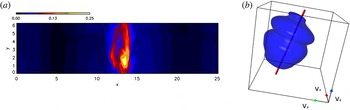
In order to appreciate the structure of $\unicode[STIX]{x1D716}$ in the spatial domain, figure 10(a) shows the contour plot of $\unicode[STIX]{x1D716}(x,y,t)$ at the time instant $t=70.7$ (when $\unicode[STIX]{x1D716}$ reaches its maximum value). The $\unicode[STIX]{x1D716}$ contours are correlated with the current structures and with the anisotropic/non-gyrotropic regions. Moreover, a blob-like region, where $\unicode[STIX]{x1D716}$ reaches its maximum, is present. This area is associated with the region where the temperature anisotropy moves from $T_{\bot }/T_{\Vert }<1$ values towards $T_{\bot }/T_{\Vert }>1$ ones (see figure 7 c). In this area the VDF strongly departs from the Maxwellian. Figure 10(b) shows the three-dimensional isosurface plot of the VDF at $t=70.7$ and in the spatial point $(x^{\ast },y^{\ast })$ where $\unicode[STIX]{x1D716}(x^{\ast },y^{\ast },t=70.7)=\max _{(x,y)}\unicode[STIX]{x1D716}(x,y,t=70.7)$ . A strong beam, parallel to the local magnetic field direction, is observed in the VDF in figure 10. The drift speed of the beam is approximately $\tilde{c}_{A}$ . The production of a beam due to the interaction of two wave packets has also been pointed out by He et al. (Reference He, Tu, Marsch, Chen, Wang, Pei, Zhang, Salem and Bale2015).