1. Introduction
The demand for robots is increasing for several industrial applications. Consequently, the larger the number of robots being use, the higher the energy consumption. However, such high levels of energy consumption can significantly affect the financial payback period of industrial robots and the sustainability of the manufacturing process [Reference Gadaleta, Pellicciari and Berselli1]. Automatizing has increased the number of robots to carry out many tasks in the industry around the world. The International Federation of Robotics (IFR) published records in
 $2018$
, where
 $2.4$
million robots were in operation worldwide, and this number has increased by approximately
 $15\%$
. IFR expects that by
 $2021$
,
 $3.8$
million industrial robots will be operating globally.
Commonly, energy generation depends on fossil energy resulting in severe pollution problems and climate change [Reference Liu and Liu, ed.)2]. Recently, new consortiums between research groups have been formed, such as the Cooperative Effort on Process Emission in Manufacturing (CO2PE), whose goal is to improve a wide range of available and emerging manufacturing processes concerning polluting emissions [Reference Kellens, Dewulf and Duflou3]. The studies of CO2PE are based on the optimization of the energy consumption of industrial robots to mitigate the emission levels of
 $CO_{2}$
and thereby reduce the environmental problems caused by industrial robots. Therefore, it is important to study and optimize the operation of industrial robots to reduce energy consumption in industry and mitigate the effects of climate change.
Industrial robots are programmed to define certain trajectories, which renders automation of industrial processes possible. The trajectories are programmed to produce new products or to adapt to changes in the production lines [Reference Gleeson, Björkenstam, Bohlin, Carlson and Lennartson4]. Moreover, the trajectory optimization provides a great opportunity to reduce energy consumption, where short and fast robot trajectories help to achieve efficient production and save energy. Considering elements of lower weight and size in the final part of industrial robot architectures has been essential as optimization criteria. In the literature, several methods have been proposed to minimize the energy consumption of industrial robots. These methods can be categorized according to the following three principal criteria:
-
1. Operation of industrial robots:
-
the required energy to perform tasks [Reference Pellicciari, Berselli, Leali and Vergnano5–Reference Kim7]
-
trajectory and run-time analysis [Reference Luo, Li, Liu and Liu8–Reference Xie, Stol and Xu11],
-
definition of the work space [Reference Ceccarelli and Lanni12–Reference Nelson, Laribi and Zeghloul14],
-
the dynamic behavior conditions [Reference Brossog, Kohl, Merhof, Spreng and Jörg15–Reference Olvander, Feng and Holmgren17],
-
control conditions [Reference Cheng and Hu18, Reference Torres and Méndez19],
-
the values of index manipulation [Reference Sánchez-Alonso, González-Barbosa, Castañeda and García Murillo20, Reference Song, She, Wang and Su21].
-
-
2. Optimization criteria for the functioning of industrial robots [Reference Rubio, Llopis-Albert, Valero and Suñer22]:
-
the minimum time required to perform the tasks, which are limited by the amount of production,
-
the minimum jerk or pull that is defined by the quality of the work and the accuracy,
-
the minimum consumed energy or minimum effort of the actuator,
-
the combined case is defined by the minimum time and energy.
-
-
3. Methods for obtaining the parameters that minimize the energy consumption. There are two categories: methods implemented in hardware and methods implemented in software. These categories are described in detail in the following list [Reference Carabin, Wehrle and Vidoni23]:
-
(a) Methods based on hardware: these involve designing and implementing components and elements for energy storage such as pneumatic, hydraulic, capacitors, and inertial flywheels. In some cases, authors have reduced the weight of components and relocated the actuators closer to the base of the robot.
-
(b) Methods based on software: these consider the optimization of trajectories and the reprogramming of operations and movements as study subjects. The following criteria were used in this category: (a) trajectory optimization algorithms, (b) analysis of energy losses by mechanical and electrical components, (c) smoothing equations such as triangular velocity, (d) cyclonic displacement, polynomial, harmonic, or modified trapezoidal and sinusoidal equations; and (e) those that define an objective function to minimize.
-
On the other hand, there have been proposals whose goal was to evaluate the energy consumption in industrial robots during their operation using different methodologies and parameters [Reference Ystgaard, Gjerstad, Lien and Nyen24–Reference Othman, Belda and Burget26]. For example, an analysis of energy consumption using the characteristics and model of an industrial robot [Reference Liu, Liu, Yao, Xu and Yang27], ABB IRB 1200 aiming to model the energy consumption when the industrial robot operated, and to analyze the trajectory that could be optimized without physical changes.
Recently, several approaches have been proposed to analyze the energy consumption of production lines where industrial robots operate simultaneously. Typically, this process is referred to as robotic cell, where the robots work synchronously with others to avoid waiting times and collisions. In ref. [Reference Eskandary, Belzile and Angeles28], the authors introduced a novel method of trajectory planning with cycle time and path constraints. The cycle time of the robot task plays a crucial role in its performance. In pick-and-place robots, the user can modify the trajectory by minimising the kinetic energy of the system and removing the actuator torque peaks by synthesizing a trajectory with smooth blendings. In addition, savings in energy consumption can be achieved using a single robot or a robotic cell [Reference Barenji, Liu, Guo and Li29, Reference Nguyen and Boveiri30].
The approach reported in ref. [Reference Riazi, Wigström, Bengtsson and Lennartson31] proposes a sequence to reduce the energy consumption of individual and interactive robots in a workstation without changing the original routes or the total cycle time. The optimization problem is formulated to minimize the weighted square angular accelerations on all joints and to approximate the energy consumption measure. The energy optimization proposed in ref. [Reference Mohammed, Schmidt and Wang32] is based on the selection of the joint configurations of a robot that consume the least energy. This energy consumption optimization was tested during the assembly task, and it was influenced by robot kinematics, dynamics, task requirements, and the technical features of robots in terms of design. The work presented in ref. [Reference Bukata, Scha, Hanzálek and Burget33] optimizes the robotic energy cells based on a mathematical model and optimization algorithms. The primary objective was to minimize the energy consumption of the robotic cell at a particular production rate by changing the robot speed, positioning, and order of operations.
Currently, some techniques have considered the type of actuators or links in the manipulator to achieve certain benefits in terms of energy consumption. For example, the work developed by ref. [Reference Nurmi and Mattila34] considered a serial manipulator with three degrees of freedom activated by hydraulic actuators. In this case, the primary objective was to minimize the cost function of the hydraulic energy consumption. Links with springs in parallel exploiting the advantage of their restitution are being employed for prosthetics and walking robots [Reference Bukata, Scha, Hanzálek and Burget33]. In fact, in ref. [Reference Plooij and Wisse35] a 2R serial prototype was developed using this principle, achieving energy savings of approximately
 $20\%$
.
In this article, we propose a methodology that efficiently reduces the energy consumption of industrial robots. Thus, our goal was to determine the best architecture for a 3R manipulator of general geometry. The 3R manipulator of general geometry can present several architectures. However, there is an optimal architecture that performs the programmed task efficiently. The architecture of industrial robots depends on the torsion angles as kinematic factor. The kinematic factors involve the design parameters: (a) lengths of links, (b) joint angles, and (c) torsion angles. Changing the lengths of links can considerably affect the energy consumption during the operation of industrial robots, as well as the structural stability and consequently the accuracy and the workspace to perform the industrial tasks, whereas the joint angles are the parameters that define the movement of an industrial robot. Finally, the torsion angles directly affect the workspace and dynamic behavior of the robot without generating significant inertial or stability problems. Therefore, these angles are the most feasible parameters for analysis in our approach.
In our approach, we varied the torsion angles according to a domain to define the search space of the architectures. The differential evolution (DE) algorithm was implemented to determine the best architecture, which ensures that energy is used efficiently for industrial robots. This proposal is based on ref. [Reference Shiakolas, Conrad and Yih36], which determined the impact of the design parameters on the accuracy, repeatability, and dynamic behavior. Furthermore, the idea to vary the torsion angles was inspired by the work of refs. [Reference Tsai and Soni13, Reference Shiakolas, Conrad and Yih36, Reference Ibrahim and Tiehu37].
However, our proposal presents analytical models whose solution is in closed form. Thus, the complexity of control algorithms is reduced. We explain in detail the design of the adaptive prototype, where we consider that our approach may provide new advantages for the use of adaptive robots in the industry. The advantages of using this adaptive robot enabled the monitoring of its dynamic behavior, and therefore, the energy consumption could be estimated. Further, the dynamic behavior was analytically validated by dynamic models that support energy consumption.
The rest of the paper is organized as follows: Section 2 shows the proposed methodology. Section 3 describes the design of the experimental adaptive prototype, which can vary its design parameters
 $\alpha$
. Section 4 shows the robot constraints and offers a method to define the path of the end effector. Section 5 describes a general geometry manipulator’s parameter design and kinematic analysis. In the same section, we present the dynamic analysis necessary for the characterization of the manipulator. Sections 6 and 8.2 offer a comparison between the experimental and analytical results. Section 7 describes the optimization process used to obtain the
 $\alpha$
values that minimize the energy consumed for specific trajectories. Section 8 shows the analytical and experimental results. Finally, we present an exhaustive discussion of the results and future work, and the conclusions of the work are in Sections 9 and 10, respectively.
2. Description of the proposed approach
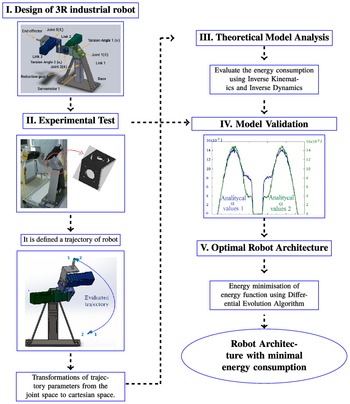
Figure 1 presents an overview of the proposed methodology. The proposed method consists of four stages to obtain the optimal parameters, which define a minimal energy consumption for a given trajectory of the robot. The first contribution is the flexible architecture design for a 3R industrial robot as presented in Section 3. This architecture allows us to modify the torsion angles parameters
 $\alpha _{1}$
and
 $\alpha _{2}$
. The second contribution is the calculation of the vector of angular acceleration, vector of torques for centrifugal effect, and the vector of torques of gravitational forces values using a theoretical model. This theoretical model is obtained from inverse and direct kinematics and inverse dynamics. The theoretical and experimental energy consumption curves are compared to validate the proposed theoretical model. We use the theoretical model to obtain the optimal parameters for the torsion angles
 $\alpha _{1}$
and
 $\alpha _{2}$
using an optimization process. A differential evolution algorithm is implemented to estimate these parameters.
Proposed approach diagram.

3. Design of 3R industrial robot
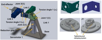
Figure 2 shows the three fundamental mechanical parts of the experimental prototype design process, listed as follows: (1) the base, (2) the links (including manufacturing and devices that allow variations between
 $\alpha$
angles), and (3) joints. The base of the experimental prototype consists of a 3.4 mm thick stainless steel blade. The design of the base is to properly install the servo-reducer system, which provides stability and functionality to perform the tasks. The top right of Fig. 2 shows the design of the experimental prototype links. Note that the links are based on
 $1/4$
”(6.35 mm) thick and 4” (101.6 mm) wide aluminum profile.
Left: CAD design of 3R adaptive prototype. Right top: CAD design for link coupling, which allows the variation and adjustment of the torsion angles
 $\alpha$
. Right bottom: joint tightening and clamping system.

The links were not only the foundation for the union between these and the servo-reducer systems, but also allowed the variation between the torsion angles
 $\alpha$
(design angles). This variation is possible due to the machined grooves as shown in Fig. 2 (upper right). However, although the tracks and machining allow for rotation to vary the torsion angles
 $\alpha$
, the design contemplates the adaptation of high-resolution rotary encoders necessary for accurate registration.
The joints between the links were directly assembled using the servo-reducer system for each link, as shown in Fig. 2, right bottom. Each of the joints must allow free movement between links, thereby ensuring that the fastening to the servo-reducer system has the least possible ‘slip’ or overlap at the moment of rotation. Moreover, improper clamping between the links and the output shaft of the speed reducer can generate an overlap. Fig. 2, bottom right, shows the clamping devices for both the first link (J1) and for the second and third links (J2). The first link handles the movement of the entire system because it handles the total weight of the prototype. Therefore, the speed reducer contained therein is reinforced to a greater extent than the other two speed reducers. In addition, the output shaft has a larger diameter and an additional keyway (machining), as shown in Fig. 2, bottom right (J1). For the second and third links, adequate clamping was achieved only via tightening, using the concepts shown in Fig. 2, bottom right (J2).
4. Experimental test
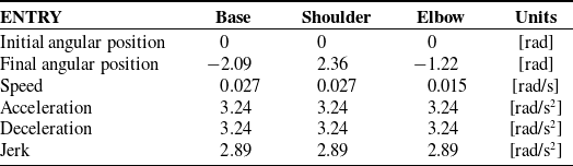
The trajectory for the analytical and experimental studies was defined based on the angular position values assigned for each of the three servomotors of the prototype, as shown in Table I. The kinematic values assigned were the same in each servomotor for the trajectory used, except for the final angular position. Furthermore, the values defined for acceleration, deceleration, and over-acceleration (jerk) were selected based on trial and error to obtain a soft behavior for the execution of the cycle.
Kinematic values for the execution of experimental prototype tests.

The angular position values were obtained from the sampling performed by the software. The domains for selecting the evolution of the position values are as follows:
 $0 \leq \theta _{1} \leq -2.09$
,
 $0 \leq \theta _{2} \leq 2.36$
, and
 $0 \leq \theta _{3} \leq -1.22$
rad. The angular position values are listed in Table I.
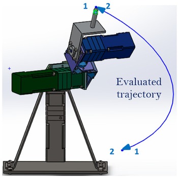
We used direct kinematics to change from joint space to Cartesian space. The coordinates defined in Cartesian space represent the trajectory evaluated using an analytical procedure. The trajectory is defined as
 $p(t) = [f_{x}(\theta _{1},\theta _{2},\theta _{3}), f_{y}(\theta _{1},\theta _{2},\theta _{3}), f_{z}(\theta _{2},\theta _{3})]^{T}$
. Figure 3 shows the evaluated trajectory performed by the end effector of the prototype, which presents a complete cycle. The trajectory starts from top to bottom and concludes with its return.
CAD design of 3R experimental prototype.

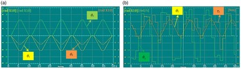
We used the input kinematic values previously defined in Table I to activate the prototype and evaluate the behavior of each servomotor. Figures 4(a), and 4(b) illustrate the angular behavior and angular dynamics of the prototype, respectively. Figure 4(a) presents the angular behavior,
 $\theta (t)$
, of the three joints in the experimental prototype. The curves were obtained using the signal generated by the oscilloscope included in the ACR-View software. The graphs show the behavior of five run cycles. The complete dynamic behavior of the second axis of the experimental prototype is shown in Fig. 4(b).
(a) Angular behavior
 $\theta (t)$
of the three joints of the experimental prototype during the path of the established trajectory. (b) Angular dynamic behavior
 $\theta (t), \dot{\theta (t)}, \tau (t)$
of the experimental prototype during operation of the shoulder, axis 2.

The software implemented for the control and movement of each servomotor allowed to obtain the angular values
 $\theta (t), \dot{\theta }(t), \tau (t)$
, discretized for the established trajectory. The angular position, speed, and acceleration values were obtained via included encoder in each servomotor, while the torque was indirectly measured using the encoder-servo amplifier through electricity consumption.
For each cycle, approximately 300 data were obtained for each angular value. As indicated, the trajectory was defined through the initial and final angular values of
 $\theta _{1},\theta _{2}$
, and
 $\theta _{3}$
, as described in Table I. The values of the remaining kinematic parameters necessary for the execution of the trajectory are assigned as average values to achieve the movement of each servomotor. For simplicity, the definition of the trajectory was based on the space of the joints of the experimental prototype. This implies avoiding the definition of the trajectory in the Cartesian space and, therefore, the need for additional analysis of the working space of the manipulator (analysis outside the subject of study in this paper).
The experimental graphs include angular position
 $\theta (t)$
, angular velocity
 $\dot{\theta }(t)$
, and torque
 $\tau (t)$
. For the angular position
 $\theta (t)$
, the cycles were uniform. However, in the case of
 $\dot{\theta }(t)$
and
 $\tau (t)$
, the curves differ between cycles. The angular position was estimated by software, with a trapezoidal profile: this factor as well as the mechanical and operational factors of the prototype which will be described in Section 9 are the cause of these differences. These irregularities are appreciated in the horizontal segment of each trapezoidal profile where its derivative, the angular velocity, should be zero (Fig. 4(b)).
Each cycle had a duration of 9 s, while the total number of records was equivalent to
 $33$
measurements per second. The time intervals between each record varied between
 $0.016$
and
 $0.042$
s. Table II shows a small sampling of the six data records, which clearly defines non-uniform sensing according to time intervals. For example:
 $\Delta _{t1} = 55.231 - 55.208 = 0.023{\,\rm s}$
,
 $\Delta _{t2} = 55.257 - 55.231 = 0.026{\,\rm s}$
,
 $\Delta _{t3} = 55.288 - 55.257 = 0.031{\,\rm s}$
,
 $\Delta _{t4} = 55.318 - 55.288 = 0.030{\,\rm s}$
, and
 $\Delta _{t5} = 55.340 - 55.318 = 0.022{\,\rm s}$
.
Random sampling of the prototype data record.

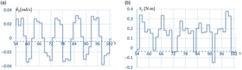
The inconsistency in the sampling time between data was one of the causes that generated irregular curves and discrepancy between cycles for angular velocity and torque curves, as shown in Figs. 4(b) and 5. In Fig. 5, each of these experimental curves for axis
 $2$
are shown individually.
Curves of dynamic behavior during experimental prototype sensing for the shoulder, axis 2: (a) Angular velocity, and (b) Torque.

5. Theoretical model analysis
5.1. Kinematics of the 3R manipulator of general geometry
Typically, industrial robots are structured by six degrees of freedom: the first three define positioning in space, while the remaining defines the orientation of objects. Moreover, the first three degrees of freedom are responsible for manipulating most of the weight of the robot, therefore the importance of the selected configuration in this study.
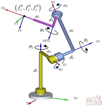
3R Serial manipulator of general geometry, distal notation of D–-H, model generated in ADEFID software [Reference González-Palacios39].

The kinematic analysis of the 3R manipulator of general geometry is based on the distal notation of Denavit–Hartenberg D–H used in ref. [Reference Peiper38] for the modeling of serial manipulators, as shown in Fig. 6. The distal notation indicates that each joint has a coordinate system defined by four design parameters: two longitudinal parameters
 $a$
and
 $d$
, and two angular parameters
 $\alpha$
and
 $\theta$
. The homogeneous transformation matrix
 $^{i-1}A_{i}$
is expressed as Eq. (1), which describes the relationship between the coordinate systems
 $(i-1)$
-th and
 $i$
-th. Figure 6 shows the parameters and characteristics defined by D–H notation.
 \begin{equation} ^{i-1}A_{i} = \begin{bmatrix} c_{i}\;\;\;\; & -s_{i}\lambda _{i}\;\;\;\; & s_{i}\mu _{i}\;\;\;\; & a_{i}c_{i} \\[5pt] s_{i}\;\;\;\; & c_{i}\lambda _{i}\;\;\;\; & -c_{i}\mu _{i}\;\;\;\; & a_{i}s_{i} \\[5pt] 0\;\;\;\; & \mu _{i}\;\;\;\; & \lambda _{i}\;\;\;\; & d_{i} \\[5pt] 0\;\;\;\; & 0\;\;\;\; & 0\;\;\;\; & 1 \\[5pt] \end{bmatrix} \end{equation}
where
 $a_{i}$
is the length of the link
 $i$
,
 $d_{i}$
is the distance to the joint
 $i-1$
,
 $\theta _{i}$
is the
 $(i-1)$
-th joint angle,
 $s_{i}$
is equal to sin(
 $\theta _{i}$
),
 $c_{i}$
is equal to cos(
 $\theta _{i}$
),
 $\alpha _{i}$
is the
 $i$
-th torsion angle between the
 $i$
-th and
 $(i-1)$
-th,
 $\lambda _{i}$
is equal to cos(
 $\alpha _{i}$
), and
 $\mu _{i}$
is equal to sin(
 $\alpha _{i}$
).
Equation (1) indicates the relationship between consecutive links which include the base or fixed coordinate system. Equation (2) shows the relationship between the pose of the end effector and the base.
 \begin{equation} ^{0}A_{p} = \begin{bmatrix} r_{1,1}\;\;\;\; & r_{1,2}\;\;\;\; & r_{1,3}\;\;\;\; & f_{x}^{0} \\[5pt] r_{2,1}\;\;\;\; & r_{2,2}\;\;\;\; & r_{2,3}\;\;\;\; & f_{y}^{0} \\[5pt] r_{3,1}\;\;\;\; & r_{3,2}\;\;\;\; & r_{3,3}\;\;\;\; & f_{z}^{0} \\[5pt] 0\;\;\;\; & 0\;\;\;\; & 0\;\;\;\; & 1 \end{bmatrix} \end{equation}
where
-
 $^{0}A_{p}$
is the end effector posture with respect to fixed coordinate system.
-
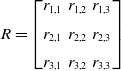
$ R = \begin{bmatrix} r_{1,1} & r_{1,2} & r_{1,3} \\[5pt] r_{2,1} & r_{2,2} & r_{2,3} \\[5pt] r_{3,1} & r_{3,2} & r_{3,3} \end{bmatrix}$
is the matrix of rotation of the end effector with respect to the fixed coordinate system.
-
$f_{x}^{0},f_{y}^{0}$
and
$f_{z}^{0}$
represent coordinates of the position of the end effector related to the fixed coordinate system.



To determine the equation for modeling the inverse kinematics of the 3R manipulator of general geometry, Eqs. (1) and (2) are combined:
 \begin{equation} ^{0}A_{p} = \underbrace{ ^{0}A_{1}{^{1}A_{2}}{^{2}A_{3}}}_{\mathbf{B}} \end{equation}
where
 $\mathbf{B}$
is the product of the matrices
 $^{0}A_{1}{^{1}A_{2}}{^{2}A_{3}}$
.
 $\mathbf{B}$
is equivalent to
 $^{0}A_{p}$
. The proposed solution is based on the positioning vectors located in the fourth column of matrices
 $\mathbf{B}$
and
 $^{0}A_{p}$
. Further, a positioning vector for time
 $t$
that defines the trajectory that executes the end effector is indicated as follows:
 \begin{equation} p(t) = \left [ \begin{array}{ccccc} f_{x} (\theta _{1}, \theta _{2}, \theta _{3}) & & f_{y}(\theta _{1}, \theta _{2}, \theta _{3})& & f_{z}(\theta _{2}, \theta _{3}) \end{array} \right ]^T, \end{equation}
Let
 \begin{equation} \vec{r}_{p}^{0} = \left [ \begin{array}{ccccc} f_{x}^{0} & & f_{y}^{0} & & f_{z}^{0} \end{array} \right ]^T, \end{equation}
and
 \begin{equation} \vec{r}_{\mathbf{B}} = \left [ \begin{array}{ccccc} f_{x} (\theta _{1}, \theta _{2}, \theta _{3}) & & f_{y}(\theta _{1}, \theta _{2}, \theta _{3}) & & f_{z}(\theta _{2}, \theta _{3})\end{array} \right ]^T, \end{equation}
Let the positioning vector be defined by the fourth column of
 $A^{(0)}_{p}$
and
 $\mathbf{B}$
, respectively.
 $\vec{r}_{\mathbf{B}}$
is defined by the following system of equations:
 \begin{align*} f_{x}(\theta _{1},\theta _{2},\theta _{3}) &= (s_{1}\mu _{1}\mu _{2} - c_{1}s_{2}\lambda _{2} - s_{1}\lambda _{1}c_{2}\lambda _{2})a_{3}s_{3}+ (c_{1}c_{2}-s_{1}\lambda _{1}s_{2})a_{3}c_{3} \\[5pt] &\quad + (c_{1}s_{2}\mu _{2} + s_{1}\lambda _{1}c_{2}\mu _{2} + s_{1}\mu _{1}\lambda _{2})d_{3} + c_{1}a_{2}c_{2} - s_{1}\lambda _{1}a_{2}s_{2}+s_{1}\mu _{1}d_{2}+ a_{1}c_{1} \end{align*}
 \begin{align} f_{y}(\theta _{1},\theta _{2},\theta _{3}) &= (c_{1}\lambda _{1}c_{2}\lambda _{2}-s_{1}s_{2}\lambda _{2}-c_{1}\mu _{1}\mu _{2})a_{3}s_{3}+ (s_{1}s_{2}\mu _{2}-c_{1}\lambda _{1}c_{2}\mu _{2}-c_{1}\mu _{1}\lambda _{2})d_{3}\nonumber \\[5pt] &\quad + (s_{1}c_{2}+c_{1}\lambda _{1}s_{2})a_{3}c_{3}+s_{1}a_{2}c_{2}+c_{1}\lambda _{1}a_{2}s_{2}- c_{1}\mu _{1}d_{2}+a_{1}s_{1} \end{align}
 \begin{align*} f_{z}(\theta _{2},\theta _{3}) &= (\mu _{1}c_{2}\lambda _{2}+\lambda _{1}\mu _{2})a_{3}s_{3}+\mu _{1}s_{2}a_{3}c_{3}+d_{1} \\[5pt] &\quad +(\lambda _{1}\lambda _{2}-\mu _{1}c_{2}\mu _{2})d_{3} +\mu _{1}a_{2}s_{2} + \lambda _{1}d_{2} \end{align*}
where
 $s_{1}$
,
 $s_{2}$
,
 $s_{3}$
,
 $c_{1}$
,
 $c_{2}$
,
 $c_{3}$
represent the trigonometric functions (sine and cosine) of the joints
 $\theta _{1},\theta _{2}$
, or
 $\theta _{3}$
, and
 $f_{x}^{0} = f_{x}(\theta _{1},\theta _{2},\theta _{3})$
,
 $f_{y}^{0} = f_{y}(\theta _{1},\theta _{2},\theta _{3})$
, and
 $f_{z}^{0} = f_{z}(\theta _{2},\theta _{3})$
. For the case that
 $\lambda _{i} = \text{cos}(\alpha _{i})$
and
 $\mu _{i}= \text{sin}(\alpha _{i})$
, were already described in Eq. (1). The positioning of the
 $z$
axis, defined as
 $f_{z}(\theta _{2},\theta _{3})$
is independent of the joint variable
 $\theta _{1}$
because this variable only describes the turn of the manipulator around its own axis; therefore, it does not affect the
 $z$
coordinate of the end effector. Consequently, this property allowed the development of the methodology proposed in ref. [Reference Peiper38].
Equation (7) presents the system of equations for calculating the inverse kinematics of the proposed prototype. The solution of the system of equations has been calculated using Pieper’s methodology [Reference Peiper38, Reference Craig40], which obtains a fourth-degree polynomial, as a function of the joint variable
 $\theta _{3}$
. This fourth-degree polynomial was solved as indicated in refs. [Reference King41, Reference Shmakov42]. Furthermore, the solution of the joint variables
 $\theta _{1}$
and
 $\theta _{2}$
, depends on the value obtained for
 $\theta _{3}$
, and is based on the analysis and solution of the quadratic equations. Consequently, four solutions for
 $\theta ^{\{1,2,3,4\}}_{3}$
were obtained using this calculation. Therefore, each solution of
 $\theta ^{j}_{3}$
corresponds to a set of solutions
 $\{ \theta ^{j}_{1}, \theta ^{j}_{2},\theta ^{j}_{3}\}$
which is described in the following section.
5.1.1. Analysis subsequent to inverse kinematics solution
Multiple kinematic solutions are considered where programing of an industrial robot movements to locate the end effector in the desired position. For the initial position, the manipulator randomly selected a solution of the four possible solutions of
 $\{ \theta ^{j}_{1}, \theta ^{j}_{2},\theta ^{j}_{3}\}$
in order to obtain the next position of the end effector using Algorithm 1.
Relationship between velocities, angular and Cartesian, for serial manipulators, based on the Jacobian matrix.


where
 $i$
defines the total of the joint variables
 $\theta _{1},\theta _{2},\theta _{3}$
, and
 $j$
indicates the maximum number of real solutions (
 $4$
for the 3R case). In addition, the PS superscript refers to the previous solution, and the value
 $\epsilon$
depends on the distance of the current position from the previous position. The previously selected solution determines a part of the subsequent solution. The process of selecting the best sequence involves reducing this value so that the architecture of the manipulator is restricted to minimal changes when its end effector moves from one point to another along of the indicated trajectory, thus avoiding sudden changes.
5.1.2. Implementation of the inverse kinematics solution: Velocities and accelerations
Kinematic analysis is the basis for the manipulator simulation and control. In this section, the kinematic process is presented, and the inverse kinematics solutions
 $(\theta _{1},\theta _{2},\theta _{3})$
are implemented to estimate the behavior of the angular velocity
 $( \dot{\theta _{1}}, \dot{\theta _{2}}, \dot{\theta _{3}})$
and angular acceleration
 $( \ddot{\theta _{1}}, \ddot{\theta _{2}}, \ddot{\theta _{3}})$
. The behavior of angular speeds and accelerations during the trajectory of a path defined by
 $p(t) = [f_{x}(\theta _{1},\theta _{2},\theta _{3}), f_{y}(\theta _{1},\theta _{2},\theta _{3}),$
 $f_{z}(\theta _{2}, \theta _{3})]^{T}$
, facilitates the start of the dynamic analysis. The Jacobian matrix
 $J_{p}$
described in Eq. (8) was obtained from the partial derivatives of the position
 $(f_{x}, f_{y}, f_{z})$
with respect to the joint variables
 $(\theta _{1},\theta _{2},\theta _{3})$
.
 \begin{align} J_{p} = \begin{bmatrix} \dfrac{\partial f_{x}}{\partial \theta _{1}}\;\;\;\; & \dfrac{\partial f_{x}}{\partial \theta _{2}}\;\;\;\; & \dfrac{\partial f_{x}}{\partial \theta _{3}} \\[12pt] \dfrac{\partial f_{y}}{\partial \theta _{1}}\;\;\;\; & \dfrac{\partial f_{y}}{\partial \theta _{2}}\;\;\;\; & \dfrac{\partial f_{y}}{\partial \theta _{3}} \\[12pt] \dfrac{\partial f_{z}}{\partial \theta _{1}}\;\;\;\; & \dfrac{\partial f_{z}}{\partial \theta _{2}}\;\;\;\; & \dfrac{\partial f_{z}}{\partial \theta _{3}} \end{bmatrix} \end{align}
The Jacobian matrix
 $J_{p}$
relates the joint velocities with the Cartesian velocities, as shown in Fig. 7, where
 $v_{x},v_{y},v_{z}$
are the Cartesian velocities.
The estimation of the angular velocities is defined by Eq. (9), where the inverse Jacobian matrix is used with the Cartesian velocities employed in vector form.
 \begin{equation} \begin{bmatrix} \dot{\theta _{1}} \\[5pt] \dot{\theta _{2}} \\[5pt] \dot{\theta _{3}} \end{bmatrix} = [J_{p}^{-1}] \begin{bmatrix} v_{x} \\[5pt] v_{y} \\[5pt] v_{z} \end{bmatrix} \end{equation}
The joint accelerations are defined via Eq. (10), where
 $\dot{J}_{p}$
represents the derivative as a function of time of the Jacobian matrix, and
 $(a_{x},a_{y},a_{z})^{T}$
represents the acceleration vector in Cartesian coordinates.
 \begin{equation} \begin{bmatrix} \ddot{\theta _{1}} \\[5pt] \ddot{\theta _{2}} \\[5pt] \ddot{\theta _{3}} \end{bmatrix} = [J_{p}^{-1}] \left (\begin{bmatrix} a_{x} \\[5pt] a_{y} \\[5pt] a_{z} \end{bmatrix} + \dot{[J_{p}]} \begin{bmatrix} \dot{\theta _{1}} \\[5pt] \dot{\theta _{2}} \\[5pt] \dot{\theta _{3}}\end{bmatrix}\right ) \end{equation}
Algorithm 2 describes the implementation of the inverse kinematics solution, which summarizes the kinematic process. It is necessary to analyze the manipulator during the tracking of the trajectory of the end effector.

Industrial robots are programmed to plan their movements at a constant velocity; however, they require acceleration at the beginning of the movement. When reaching their final position, they are required to decelerate until they stop. It is often essential to use cycloidal, polynomial, harmonic, or trapezoidal and sinusoidal displacement equations to soften the velocity. Consequently, changes in acceleration and deceleration are minimizad. Furthermore, the energy consumption decreases with better acceleration control and deceleration changes during the path of the end-effector trajectory. In the middle part of the trajectory, the Cartesian velocity of the end effector is the optimum constant to achieve lower-energy wastage [Reference Barrientos, Peñin, Balaguer and Aracil43].
Kinematic analysis presents the study of movement, whereas dynamic analysis aims to study the relationship between movement and the forces involved. Therefore, kinematic and dynamic analysis are complimentary for the characterization of the manipulator behavior. In the next section, a dynamic analysis is presented.
5.2. Dynamics for 3R manipulator of general geometry
The dynamic analysis of the 3R manipulator with variations in the torsion angles
 $\alpha _{1}$
and
 $\alpha _{2}$
is based on the formulation of Lagrange, The subsequent kinematics of the manipulator are defined from two different perspectives of evaluation: (a) the inverse dynamics and (b) the direct dynamics. For this analysis, the inverse dynamics expresses the forces and torques in the function of the temporal evolution of the joint variables and derivatives, as shown in Fig. 8.
Relationship between inverse dynamics and direct dynamics for serial manipulators.

The dynamic model is a complex problem in the analysis of manipulators due to its nonlinear behavior. This model is essential in ref. [Reference Barrientos, Peñin, Balaguer and Aracil43]:
-
Simulation of movement of the robot,
-
The design and evaluation of the mechanical structure of the robot,
-
The selection of actuators,
-
The design and evaluation of the dynamic control of the robot.
The dynamic model of the manipulator is defined via inverse dynamics, which defines the torque required in each joint to execute the movement.
5.3. Inverse dynamics: Lagrange formula
The Lagrange formula in the dynamic model of the robots was based on the kinetic and potential energies for each element. For each joint, the torque was obtained using the expressions indicated in Eq. (11).
 \begin{equation} \tau _{1} = \frac{d}{dt}\frac{\partial L}{\partial \dot{\theta _{1}}} - \frac{\partial L}{\partial \theta _{1}}\ ;\quad \tau _{2} = \frac{d}{dt}\frac{\partial L}{\partial \dot{\theta _{2}}} - \frac{\partial L}{\partial \theta _{2}}\ ;\quad \tau _{3} = \frac{d}{dt}\frac{\partial L}{\partial \dot{\theta _{3}}} - \frac{\partial L}{\partial \theta _{3}} \end{equation}
Friction is not included in Eq. (11). Thus, it is considered a conservative system where energy losses due to friction are not present. The Lagrangian
 $L$
is defined in Eq. (12):
 \begin{equation} L = \sum K_{i}-\sum P_{i} \end{equation}
The term
 $K_{i}$
defines the kinetic energy and is equivalent to
 $K_{b} + K_{1} + K_{2} + K_{3} + K_{C}$
, whereas
 $P_{i}$
represents the potential energy and is equivalent to
 $P_{b} + P_{1} + P_{2} + P_{3} + P_{C}$
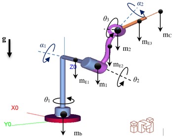
, the details of which are presented in Appendix A. The subscript
 $b$
refers to the base of the manipulator, and the mass concentrated in the middle part of each link is denoted by
 $m_{E1}$
,
 $m_{E2}$
, and
 $m_{E3}$
, while the terms
 $1$
and
 $2$
refer to the weights concentrated in the joints (servomotor-speed reducer system). Finally,
 $C$
indicates the handled load by the end effector where any tool can be used. Figure 9 presents the free body diagram of the 3R prototype of general geometry.
Free body diagram of 3R prototype of general geometry, model generated in ADEFID software [Reference González-Palacios39].

Equation (13) describes the torques generated based on dynamic terms.
 \begin{equation} \tau ={M(\theta )}{\ddot{\theta }} +{V(\theta,\dot{\theta })}+G(\theta ) \end{equation}
Where
-
$\tau$
: is the vector of torques required for the movement of the joint variables,
-
$M(\theta )$
: is the inertia matrix,
-
$\ddot{\theta }$
: is the angular acceleration vector,
-
$V(\theta, \dot{\theta })$
: is the vector of torques for centrifugal effects and Coriolis,
-
$G(\theta )$
: is the vector of torques due to gravitational forces.


For practical purposes, this study does not include the equations of torques which are obtained analytically because of their size. However, the general expression of each torque is presented in Eq. (11), as well as each of the expressions of Lagrangian
 $L$
in Appendix A. These expressions are used in the algorithm to generate dynamic behavior curves. For further details, refer to ref. [Reference Castillo and Caberta44] for the analysis and comparison of expressions based on similar studies.
6. Model validation
The transmission of speed reducers prevented to achieve an efficiency of 100%. During the prototype operation, the software and hardware only allowed the registration and simultaneous output of the four signals at most. Thus, it was not possible to obtain the six signals in one cycle,
 $(\dot{\theta _{1}}, \tau _{1}, \dot{\theta }_{2},\tau _{2},$
 $\dot{\theta }_{3},\tau _{3})$
, which are necessary for complete monitoring and estimation of power and energy consumption. Therefore, several runs were necessary in sets such as:
 $(\dot{\theta _{1}}, \tau _{1}, \dot{\theta }_{2}, \dot{\theta }_{3})$
,
 $(\dot{\theta _{2}}, \tau _{2}, \dot{\theta }_{2}, \dot{\theta }_{3})$
,
 $(\dot{\theta _{3}}, \tau _{3}, \dot{\theta }_{1}, \dot{\theta }_{2})$
,
 $(\dot{\theta _{1}}, \tau _{1}, \tau _{2}, \tau _{3})$
,
 $(\dot{\theta _{2}}, \tau _{2}, \tau _{1}, \tau _{3})$
, or
 $(\dot{\theta _{3}}, \tau _{3}, \tau _{1}, \tau _{2})$
, for example; for synchronizing and coupling the monitored cycles of the three axes.
The discretized data and records from the execution of the trajectory by the end effector are replaced in Eqs. (14) and (15), which estimate the power
 $P(t)$
and energy
 $E(t)$
consumed by the experimental prototype for each of the monitored cycles. The expressions generated from Eq. (17) are
 \begin{equation} P(t) = \sum _{j=1}^{j=n_{D}} \left [\tau _{1,t_{j}}\cdot \dot{\theta }_{1,t_{j}} + \tau _{2,t_{j}}\cdot \dot{\theta }_{2,t_{j}} + \tau _{3,t_{j}}\cdot \dot{\theta }_{3,t_{j}} \right ] \end{equation}
 \begin{equation} E(t) = \displaystyle \sum _{j=1}^{j=n_{D}} \left [(\tau _{1,t_{j}}\cdot \dot{\theta }_{1,t_{j}} + \tau _{2,t_{j}}\cdot \dot{\theta }_{2,t_{j}} + \tau _{3,t_{j}}\cdot \dot{\theta }_{3,t_{j}}) (t_{j} - t_{j-1})\right ] \end{equation}
where
 $(t_{j} - t_{j-1})$
represents the time lapse of the record between the monitored data.
6.1. Analytical and experimental evaluation of the electrical energy consumption
In this section, we present a method to evaluate the energy consumption of the prototype. The control software for the prototype, through monitoring, allows the recording of dynamic variables such as angular position, angular velocity, angular acceleration, and torque. Based on this, the energy equations to be used for the estimation of consumption, analytical-Equation (16), and experimental-Equation (17), are as follows
 \begin{equation} E = \displaystyle \int _{t_{\text{initial}}}^{t_{\text{final}}} \left [ \displaystyle \sum _{i=0}^{i=n_{s}} \left ( \tau _{i}(t)\cdot \dot{\theta _{i}}(t) \right ) \right ] dt \end{equation}
where
 $n_{s}$
represents the number of joints considered. For this case, the analytical form is defined as the integral of the developed torque
 $\tau (t)$
(see Eq. (13)) for each joint of the manipulator multiplied by its respective angular velocity
 $\dot{\theta }(t)$
during runtime. And, the equation to evaluate the energy consumption for the experimental case is expressed as:
 \begin{equation} E \cong \displaystyle \sum _{j=1}^{j=n_{D}} \left [ \displaystyle \sum _{i=0}^{i=n_{s}} \left ( \tau _{i,j}\cdot \dot{\theta }_{i,j} \right ) \right ] \Delta t \end{equation}
where the number of sampling data is written as
 $n_{D}$
,
 $\Delta _{t}$
represents the time in the sampling intervals,
 $\tau _{i,j}$
is the torque of the servomotor
 $i$
,
 $j$
, and
 $\dot{\theta }_{i,j}$
is the angular velocity of the servomotor
 $i$
in the data
 $j$
. The term
 $\tau (t) \cdot \dot{\theta }(t)$
indicates the developed potency,
 $P(t)$
.
7. Optimal robot architecture
Algorithm 3 shows the calculation of the energy consumed by the 3R manipulator of general geometry for the path to be assigned and predefined design parameters. The calculated energy was based on the design parameters
 $(\alpha _1,\alpha _2)$
. Industrial robots develop repetitive tasks with predefined trajectories. Thus, to determine the optimal design
 $(\alpha _1, \alpha _2)$
values based on the energy consumed by a robot where the path is known, the energy COMPUTED
 $\_$
ENERGY can be calculated to determine the parameters
 $(\alpha _1,\alpha _2)$
that consume the least.

8. Results
This section presents the built serial robot architecture and the numerical data validation from the experimental data, and lastly, we propose a serial robot architecture that minimizes the energy consumption for a pre-established trajectory.
8.1. Experimental test
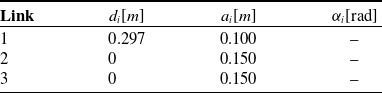
The values of the design parameters D–H for the experimental prototype are listed in Table III. However, the values of the angles
 $\alpha$
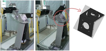
are not indicated because they may vary according to the execution. Figure 10 shows the experimental prototype. The left side of figure shows an orthogonal architecture whose values are
 $\alpha _{1} = -\pi/2$
rad,
 $\alpha _{2} = \pi$
rad, the middle figure shows an arbitrary architecture whose values are
 $\alpha _{1} = -2\pi/3$
,
 $\alpha _{2} = 7\pi/6$
rad. The design angles
 $\alpha$
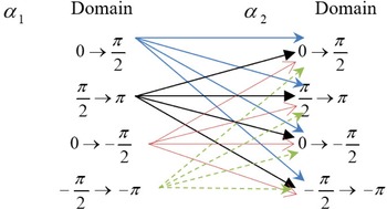
were delimited to a single quadrant for the domains:
 $-\pi/2 \leq \alpha _{1} \leq -\pi$
. Nevertheless, it can cover more than one quadrant. The orthogonal architecture is commonly used in industrial robots.
Figure 10 right shows the design of the links of the prototype, where manufactured slots are visualized to achieve the adjustment and variation of these
 $\alpha$
angles.
8.1.1. Control and movement of experimental prototype
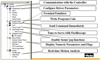
The control and movement system prototype consist of a servo amplifier (drive), controller, computer equipment, and control software. For each servomotor, a servo amplifier was required for an adequate energy supply. Further, the equipment acquired for the operation of the prototype was a digital controller ACR9640/P3/U0/B0 DC, as well as three servo-digital amplifiers Aries AR-08PE. ACR-View software was employed to control the experimental prototype. Figure 11 describes the workspace components of a project which is developed in the ACR-View software.
The option Terminal Emulator located in the workspace of the ACR-View software rendered the activation and deactivation of the servomotors and running programs defined by the user configuration. For the current project, a structured ladder logic language is necessary for the basic program of execution and monitoring of the operation of the prototype. This programing tool is located on the far right of the graphic environment of the ACR-View software and is defined as MainProgram.LDD.
The proper use of programing commands and tools can be reviewed in the programing manuals published online [45]. The source of the code that controls the movement of the prototype was written following the above-mentioned manuals. The control software used, ACR-View 6.2.0, supports libraries and applications in Visual C
 $\#$
, Microsoft.NET, LabVIEW, and Delphi languages. In addition, the communication of the control system was achieved via Ethernet Powerlink. The servomotors used were the brushless type, series SM of Parker company, and the reduction gears employed were NEMA23; the details are listed in Table IV.
Parameters D–H of experimental prototype.

3R Experimental adaptive prototype: left side, orthogonal architecture, in the middle, an arbitrary architecture, and right side, the design of the experimental prototype links for variation and adjustment of torsion angles
 $\alpha$
.

Project work space in ACR-View software.

Servomotors and reduction gears used in the experimental prototype.

The transmission used by speed reducers was the planetary gears. For the base, the speed reducer comprises reinforced bearings to support most of the weight of the prototype. The weights of the reduction gears were as follows: base (0.9 kg), shoulder (0.9 kg), and elbow (0.7 kg); further, for the servomotors, base (1.4 kg), shoulder (1.4 kg), and elbow (1.0 kg). The weights for additional elements were link 1 (0.56 kg), link 2 (0.36 kg), and link 3 (0.17 kg). These values are shown in Fig. 9 as
 $m_{E1}=0.56$
,
 $m_{E2}=0.36$
,
 $m_{E3}=0.17$
,
 $m_{c}=0$
,
 $m_{1}=1.4+0.9=2.3$
, and
 $m_{2}=1.0+0.7=1.7$
kg. The previous weights were considered for the analytical models. However, the workload is not included since the end effector is a follower in this case. In addition, for the analytical study, the backlash (15 arc-min or 0.25
 $^{\circ }$
) of the reduction gears was not considered. Furthermore, the values of static friction, 0.0021 (elbow), 0.0049 (base and shoulder) Nm, and viscous damping in servomotors 0.0000167 (elbow), 0.0000241 (base and shoulder) Nms/rad, were considered negligible.
8.2. Model validation
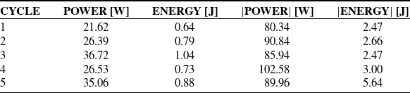
Table V indicates the total power and energy consumed by the prototype during each cycle. The use of absolute values allows the quantification of the
 $|$
POWER
 $|$
and
 $|$
ENERGY
 $|$
, avoiding negative values. The values obtained between the power and consumed energy cycles differ due to the discrepancy between records per cycle, which is reflected in the curves of angular and torque velocities in Figs. 4b and 5.
Power and energy consumption during the operation of experimental prototype.

8.2.1. Comparison: Experimental curves and analytical curves, with values
$\alpha _{1} = -\pi/2$
and
$\alpha _{2} = \pi$


The first step for the analysis of the energy consumed by the prototype was to compare the curves generated by the analytical models with those obtained experimentally. In this regard, it was necessary to verify in the following figures that a similar and consistent behavior exists between the analytical and experimental curves. The curves for both cases were generated from the input data in Table I for a previously defined trajectory. The design parameters are listed in Table III. For this case, we considered
 $\alpha _{1} = -\pi/2$
and
 $\alpha _{2} = \pi$
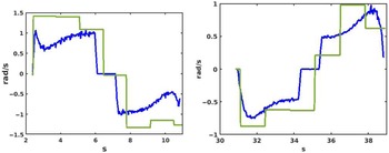
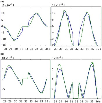
, as the architecture for analysis. Figure 12 shows the behavior of the angular velocities for axes
 $2$
and
 $3$
of the prototype. Further, the images show the analytical (calculated) and experimentally (sensed) curves. The experimental curves generally behave as square waves due to the discretisation in the monitoring and data recording. The mean-squared error between analytical and experimental data for
 $\dot{\theta }_{2}(t)$
is 0.34
 $\dfrac{rad^2}{s^2}$
, and for
 $\dot{\theta }_{3}(t)$
is 0.1
 $\dfrac{rad^2}{s^2}$
.
Angular velocities for the analytical case (blue curves) and experimental case (green curves) for the axes 2 and 3: left side
 $\dot{\theta }_{2}(t)$
, and right side
 $\dot{\theta }_{3}(t)$
. The MSE for
 $\dot{\theta }_{2}(t)$
is 0.34
 $\frac{rad^2}{s^2}$
, and for
 $\dot{\theta }_{3}(t)$
is 0.1
 $\dfrac{rad^2}{s^2}$
.

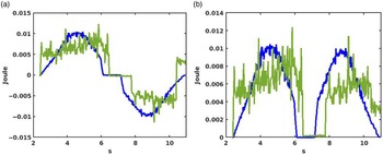
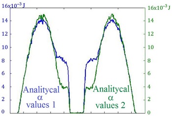
For the case illustrated in Fig. 13, the curves of the energy consumed by axis 2 were compared during the execution of a cycle. The mean-squared error between the analytical and experimental results was
 $1\times 10^{-5}$
J
 $^2$
. The previous analytical and experimental curves show similarities, indicating that the analytical models implemented can be considered suitable. The next step is to analytically validate that the energy consumption is affected by using different values of the angles
 $\alpha _{1}$
and
 $\alpha _{2}$
.
Analytical behavior (blue curves) and experimental behavior (green curves) of axis 2: (a) energy and (b) absolute energy consumed. MSE is
 $1\times 10^{-5}$
Joules
 $^2$
.

8.2.2. Comparison of analytical graphs, for two architectures: 1.
$\alpha _{1}=-1.78$
rad,
$\alpha _{2}=3.49$
rad; and 2.
$\alpha _{1}=3.49$
rad,
$\alpha _{2}=1.78$
rad


The dynamic behavior of the manipulator was analytically compared for two different pairs of
 $\alpha$
values considering the same trajectory, which was defined in the previous sections. The selected
 $\alpha$
values generated two different manipulator architectures. Moreover, the end effector can execute the trajectory in both cases. This was verified by the analysis and convergence of the inverse kinematics; so, an analysis of the manipulator workspace was not necessary. The selected
 $\alpha$
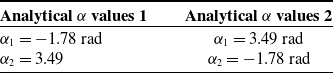
values are listed in Table VI for which the energy consumption of two different architectures executing the same task was analytically compared.
Analytical
 $\alpha$
values used in comparison of energy consumption for two architectures.

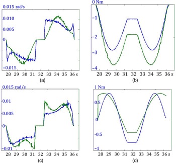
We verified that the behavior of the manipulator and its energy consumption are affected by the variation in these angles. Figure 14 shows a comparison of the angular velocity
 $\dot{\theta }(t)$
and torque
 $\tau (t)$
curves for axes 2 and 3 in both cases.
Dynamic behavior for axes 2 and 3: (a)
 $\dot{\theta }_{2}(t)$
,(b)
 $\tau _{2}(t)$
, (c)
 $\dot{\theta }_{3}(t)$
, (d)
 $\tau _{3}(t)$
. Analytical
 $\alpha$
values 1 (blue curves), and analytical
 $\alpha$
values 2 (green curves).

Figure 15 illustrates the analytical behavior of axes 2 and 3 of the manipulator in relation to energy consumption for values defined in Table VI.
Analytical behavior of the energy consumed by each axis of the manipulator with
 $\alpha$
values described in Table VI. (a) Axis 2 and (b) axis 3. Energy-left side and absolute energy-right side.

Finally, in Fig. 16, the total consumption of energy required by the manipulator during the execution of the same trajectory for both architectures has been illustrated.
Absolute value of the total energy consumption during the path of the end effector of the manipulator for
 $\alpha$
values described in Table VI. Analytical
 $\alpha$
values 1 (blue curve) and analytical
 $\alpha$
values 2 (green curve).

Figure 16 presents a direct comparison of the energy consumed values between two analytical cases. The difference of energy consumed between both cases is
 $7.5\%$
, which was calculated using the mean squared error equation. The analytical cases were realized for two different architectures of 3R manipulator using the
 $\alpha$
values presented in Table VI.
8.3. Optimal robot architecture
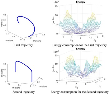
Figure 17 shows the energy consumed by the robot for a fixed range of
 $(\alpha _1, \alpha _2)$
values for two trajectories. The optimal
 $ (\alpha _1, \alpha _2)$
values obtained from this range determine the architecture that the robot should adopt for the lowest power consumption. Moreover, we used the differential evolution method [Reference Storn and Price46] to minimize COMPUTED
 $\_$
ENERGY
 $(\alpha _1, \alpha _2)$
. The optimal values of the first trajectory in Fig. 17 are:
 $\alpha _1 = -1.3925$
rad, and
 $\alpha _2= 3.0287$
rad, with a computation time of 7741.8 s. For the second trajectory, the optimal values in Fig. 17 are:
 $\alpha _1 = -1.4302$
rad and
 $\alpha _2= 3.3581$
rad, with a computation time of 14134.1 s. Algorithm 3 was programmed in MATLAB on an Intel Core i7-4770 CPU 3.4 GHz
 $\times$
8, 32 GB RAM computer.
Analyzed trajectories and energy consumption based on the variation of the
 $\alpha _1$
and
 $\alpha _2$
values.

In the right image of Fig. 17,
 $\alpha _{1}$
and
 $\alpha _{2}$
represent the first two axes, and the third axis represents the consumed energy for each trajectory. According to the convergence of the inverse kinematics solution, all possible combinations allow the end effector to execute the two established trajectories.
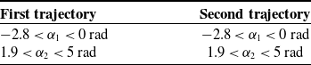
Table VII presents the domains for
 $\alpha _{1}$
and
 $\alpha _{2}$
, showed in Fig. 17, which shows two trajectories. Each trajectory is presented with its function
 $\in$
 $\mathbb{R}^{3}$
, which indicates the energy consumption. The energy function depends on the torsion angles of architectures. Consequently, this analysis enables us to determine the combination of torsion angles
 $\alpha _{1}$
and
 $\alpha _{2}$
, thereby estimating the architecture of the manipulator with lower electrical consumption during the execution of the trajectory. An optimization process based on Differential Evolution (DE) method was applied to achieve the optimal combination of torsion angles.
The optimal combination of the first and second trajectories (defined in Table VII) is as follows:
 $\alpha _{1} = -1.3925$
rad,
 $\alpha _{2} = 3.0287$
rad; and
 $\alpha _{1} = -1.4302$
rad,
 $\alpha _{2} = 3.3581$
rad, respectively. These values are close to those used in industrial robots:
 $\alpha _{1} = \pm \pi/2 (\pm 1.5708 rad)$
, and
 $\alpha _{2} = 0$
,
 $\pm \pi (\pm 3.1416 rad)$
.
The cases analyzed in Table VII contain only the local minimum estimate. There are more possible combinations of values
 $\alpha _{1}$
and
 $\alpha _{2}$
to be analyzed. Consequently, this allows us to obtain an optimal global combination. The possible combinations of values
 $\alpha _{1}$
and
 $\alpha _{2}$
must cover each of the defined octanes in the Euclidean space, for which the axes of the Cartesian space are defined by
 $\alpha _{1}$
and
 $\alpha _{2}$
. Figure 18 shows the suggested combination of values
 $\alpha _{1}$
and
 $\alpha _{2}$
to cover the total number of octanes. In this case, the number of possible combinations was 16.
It should be emphasized that the total of possible combinations of (
 $\alpha _{1}$
,
 $\alpha _{2}$
) values is restricted by the workspace of the manipulator, where the inverse kinematics solution must converge.
9. Discussion
The analytical and experimental cases for the dynamic curves were validated in Subsection 8.2.1. In both cases, the results were close and consistent, indicating that our dynamic models are appropriate. The values for the validation were
 $\alpha _{1} = \pi/2$
and
 $\alpha _{2} = \pi$
, which are commonly used in industrial robots.
Domain of the torsion angles to obtain the different combinations for Fig. 17.

Combination of (
 $\alpha _{1}$
,
 $\alpha _{2}$
) values, suggested to cover the total octanes of the Euclidean space.

Figure 16 shows that the energy consumption is different when the architecture presents different
 $\alpha$
values. According to our analytical results, the energy saved is
 $7.5\%$
less. Nowadays, a multitude of industrial robots operate continuously, therefore, minimum savings are of great importance.
Figures 4(b) and 5 show a non-uniformity between cycles of torque curves and angular velocity due to three main causes:
-
1. Data sampling was not uniform during experimentation. Table II presents an example of the data sampling where a uniform time to collect the data was not obtained. For the non-uniformity between the curves, see Figure 4(b), an interpolation process can be applied to improve dynamic profiles.
-
2. The trapezoidal profile of the angular position that internally drives the software for the control of the prototype, see Figure 4(a).
-
3. Inertial changes during the return of motion between cycles.
Regarding the optimization process, described in Section 7, it is important to highlight the proximity of the calculated values, to common values in industrial robots; which according to refs. [Reference Tsai and Soni13, Reference Ibrahim and Tiehu37] it is beneficial. This also indicates that small changes in these torsion angles can result in significant improvement of energy saving.
As previously mentioned, we consider two trajectories for this analysis. Figure 3 illustrates the first trajectory, and the second trajectory simulates a pick and place execution. For each case, we evaluate analytically several robot architectures. We evaluate each trajectory for a range of combinations of values
 $\alpha _{1}$
and
 $\alpha _{2}$
. The possible combinations of values
 $\alpha _{1}$
and
 $\alpha _{2}$
are shown in Fig. 17.
10. Conclusions
This article presents a methodology for reducing the energy consumption of industrial robots. We varied the torsion angles to build a search space of architectures for an adaptive robot, and the optimal architecture was determined using the DE algorithm. The energy consumption can vary using different architectures. However, with the use of computational approaches such as the DE algorithm as an optimization technique, it is possible to determine an optimal architecture to ensure that energy is used efficiently for industrial robots.
We also presented an analytical study of energy dynamic model consumption for an adaptive robot. The adaptive robot was designed and built by the authors, the prototype’s main concept was described in Section 4. The analytical study was experimentally validated using the proposed prototype. In addition, validation was performed using analytical and experimental dynamic curves. Both dynamic curves obtained were very similar, and the mean-squared error was on the order of
 $1\times 10^{-5}$
Joules
 $^2$
for consumption energy.
According to experimental and analytical results, it was shown that by varying the torsion angles while applying an optimization procedure, such as the DE algorithm, it was possible to obtain the best architecture for industrial robots to reduce its energy consumption. The proposed prototype is scalable and could evolve into a new industrial robot (according to the author’s knowledge, the manufacturing process is possible), offering advantages such as the minimum energy consumption for a given trajectory. The proposed robot can be reconfigured if the trajectory changes, offering optimal energy consumption for the new trajectory. Section 7 shows a methodology to compute the configuration parameters of the robot.
We presented detailed design and implementation aspects of an experimental prototype, which was an adaptive robot (3R manipulator of general geometry). Therefore, for this adaptive robot, we evaluated the energy consumption using the proposed methodology. The work presented here provides new advantages and promotes the use of adaptive robots, where this type of robot is not very common in the industry due to its high complexity and, therefore, it requires additional analysis according to its configuration such as workspace, manufacturing, and control parameters. We achieved an optimal architecture for our adaptive robot as a function of torsion angles and a trajectory to reduce energy consumption, and hence reducing energy consumption and efficiently using energy can mitigate costs and environmental problems, such as climate change.
In future work, we will combine certain techniques or proposed methodologies used in the literature to reduce energy consumption with our proposal.
Availability of data and materials
The datasets used or analyzed during the current study are available from the corresponding author on reasonable request.
Authors’ contributions
Erick-Alejandro González-Barbosa, Luz Antonio Aguilera-Cortés, and Max Antonio González-Palacios provided the original and flexible architecture design for a 3R industrial robot. José-Joel González-Barbosa used the theoretical model to obtain the optimal parameters for the torsion angles
 $\alpha _1$
and
 $\alpha _2$
using an optimization process. Juan Pablo Serrano-Rubio and José Ángel Colin Robles wrote the relevant content of the manuscript and designed the algorithm.
Conflicts of interest
The authors declare none.
Ethical considerations
All researches are based on published studies and innovative design ideas, and do not involve humans and various organisms, so they are not applicable.
Appendix A: Obtaining the Lagrangian from the 3R serial manipulator of general geometry
The Lagrangian of the manipulator under study is the basis for the analysis of the dynamic behavior. The Lagrangian is based on kinetic and potential energies. Each term contained in the expressions described here was defined in Sections 5.1 and 5.2 of this paper, in specific Eqs. (11), (12), and Fig. 9. The terms
 $x_{i}, y_{i}, z_{i}$
indicate the Cartesian positioning of each element,
 $II_{i}$
the moment of inertia of the designated element, and
 $g$
indicates the gravity.
Kinetic energy:
 \begin{equation*} K_b = 0.5 m_{b}r_b^2\dot {\theta _{1}}^2 \end{equation*}
 \begin{equation*} K_1 = 0.125 m_{E1}a_1^2\dot {\theta _{1}}^2 + 0.5 m_{1}a_1^2\dot {\theta _{1}}^2 \end{equation*}
 \begin{equation*} K_2 = 0.5 m_2 V_2^2 + 0.5 I_2\dot \theta _1^2 \end{equation*}
where
 \begin{equation*} I_2 = m_2 x_2^2 \end{equation*}
 \begin{equation*} V_2 = \sqrt {V_{x2}^2 + V_{y2}^2 + V_{z2}^2} \end{equation*}
 \begin{equation*} x_2 = a_1 + 0.5 a_2 c_{2};\qquad y_2 = 0.5 \lambda _1 a_2 s_2 - \mu _1 d_2; \qquad z_2 = 0.5 \mu _1 a_2 s_2 + \lambda _1 d_2 + d_1 \end{equation*}
Deriving
 $x_2, y_2, z_2$
as a function of time
 \begin{equation*} V_{x2} = -0.5 s_2 \dot \theta _2 \end{equation*}
 \begin{equation*} V_{y2} = 0.5 a_2 c_2 \dot \theta _2 \end{equation*}
 \begin{equation*} V_{z2} = 0.5 \mu _1 a_2 c_2 \dot \theta _2 \end{equation*}
 \begin{equation*} K_3 = 0.5 m_3 V_3^2 + 0.5 I_3\dot \theta _1^2 \end{equation*}
where
 \begin{equation*} I_3 = m_3 x_3^2 \end{equation*}
 \begin{equation*} V_3 = \sqrt {V_{x3}^2 + V_{y3}^2 + V_{z3}^2} \end{equation*}
 \begin{equation*} x_3 = 0.5 a_3 c_2 c_3 - 0.5 a_3\lambda _2 s_2s_3 + s_2 + s_2\mu _2 d_3 + a_2 c_2 +a_1 \end{equation*}
 \begin{equation*} y_3 = 0.5\lambda _1 a_3 s_2 c_3 + 0.5 a_3 \lambda _1\lambda _2c_2s_3-\lambda _1 \mu _2 d_3 c_2 - \mu _1 \lambda _2 d_3 + \lambda _1 a_2 s_2 -\mu _1 d_2 \end{equation*}
 \begin{equation*} z_3 = 0.5a_3\mu _1s_2c_3 + 0.5a_3s_3(\mu _1c_2\lambda _2+\lambda _1\mu _2) + d_3(\lambda _1\lambda _2-\mu _1\mu _2c_2)+\mu _1a_2s_2+\lambda _1d_2+d_1 \end{equation*}
Deriving
 $x_3, y_3, z_3$
as a function of time
 \begin{equation*} V_{x3} = 0.5a_3(-c_2s_3\dot \theta _3-c_3s_2\dot \theta _2)-0.5a_3\lambda _2(s_2c_3\dot \theta _3+s_3c_2\dot \theta _2)+\mu _2d_3c_2\dot \theta _2-a_2s_2\dot \theta _2 \end{equation*}
 \begin{equation*} V_{y3} = 0.5a_3\lambda _1(-s_2s_3\dot \theta _3+c_2c_3\dot \theta _2)+0.5a_3\lambda _1\lambda _2(c_2c_3\dot \theta _3-s_2s_3\dot \theta _2)+\lambda _1\mu _2d_3s_2\dot \theta _2+\lambda _1a_2c_2\dot \theta _2 \end{equation*}
 \begin{equation*} V_{z3} = 0.5a_3\mu _1(-s_2s_3\dot \theta _3+c_2c_3\dot \theta _2)+0.5\mu _1\lambda _2a_3(c_2c_3\dot \theta _3-s_2s_3\dot \theta _2)+\mu _1\mu _2d_3s_2\dot \theta _2+\mu _1a_2c_2\dot \theta _2 \end{equation*}
 \begin{equation*} K_C = 0.5 m_C V_C^2 + 0.5 I_C\dot \theta _1^2 \end{equation*}
where
 \begin{equation*} I_C = m_Cx_C^2 \end{equation*}
 \begin{equation*} x_C = a_3c_2c_3-a_3\lambda _2s_2s_3 \end{equation*}
 \begin{equation*} y_C = \lambda _1 a_3 s_2 c_3 + a_3 \lambda _1\lambda _2c_2s_3-\lambda _1 \mu _2 d_3 c_2 - \mu _1 \lambda _2 d_3 + \lambda _1 a_2 s_2 -\mu _1 d_2 \end{equation*}
 \begin{equation*} z_C = a_3\mu _1s_2c_3 + a_3s_3(\mu _1c_2\lambda _2+\lambda _1\mu _2) + d_3(\lambda _1\lambda _2-\mu _1\mu _2c_2)+\mu _1a_2s_2+\lambda _1d_2+d_1 \end{equation*}
Deriving
 $x_C, y_C, z_C$
as a function of time
 \begin{equation*} V_{xC} = a_3(-c_2s_3\dot \theta _3-c_3s_2\dot \theta _2)-a_3\lambda _2(s_2c_3\dot \theta _3+s_3c_2\dot \theta _2)+\mu _2d_3c_2\dot \theta _2-a_2s_2\dot \theta _2 \end{equation*}
 \begin{equation*} V_{yC} = a_3\lambda _1(-s_2s_3\dot \theta _3+c_2c_3\dot \theta _2)+a_3\lambda _1\lambda _2(c_2c_3\dot \theta _3-s_2s_3\dot \theta _2)+\lambda _1\mu _2d_3s_2\dot \theta _2+\lambda _1a_2c_2\dot \theta _2 \end{equation*}
 \begin{equation*} V_{zC} = a_3\mu _1(-s_2s_3\dot \theta _3+c_2c_3\dot \theta _2)+\mu _1\lambda _2a_3(c_2c_3\dot \theta _3-s_2s_3\dot \theta _2)+\mu _1\mu _2d_3s_2\dot \theta _2+\mu _1a_2c_2\dot \theta _2 \end{equation*}
Potential energy:
 \begin{equation*} P_b = 0 \end{equation*}
 \begin{equation*} P_1 = 0 \end{equation*}
 \begin{equation*} P_2 = m_2 g z_2 \end{equation*}
 \begin{equation*} P_3 = m_3 g z_3 \end{equation*}
 \begin{equation*} P_C = m_C g z_C \end{equation*}
Finally, the Lagrangian is defined as:
 \begin{equation*} L = K_b + K_1 + K_2 + K_3 + K_C - P_b - P_1 - P_2 - P_3 - P_C \end{equation*}