Introduction
The color appearance of simple stimuli can be described by three opponent dimensions that represent the relative contributions of red versus green, blue versus yellow, or bright versus dark sensations (Kaiser & Boynton, Reference Kaiser and Boynton1996). Colors of a given brightness can be arranged within a circle to characterize how they differ from the central white point, according to their saturation (distance from the neutral point) and hue (direction from white). Hue varies with the ratio of red versus green to blue versus yellow. Thus, most lights appear as a mixture of these dimensions (e.g., orange appears both red and yellow), while lights that isolate one of the axes (i.e., unique red, green, blue, or yellow) appear more pure or fundamental (Hurvich & Jameson, Reference Hurvich and Jameson1957; Hering, Reference Hering1964).
A central yet unresolved question in modern color science concerns the extent to which the perceptual organization of color in terms of a small number of primary color–opponent dimensions reflects the physiology of color coding or the properties of color signals in the environment. In biologically based models, colors that are special reflect special states in neural coding (Hurvich & Jameson, Reference Hurvich and Jameson1957; De Valois & De Valois, Reference De Valois and De Valois1993). For example, the unique hues are assumed to correspond to the null points in the spectral sensitivities of opponent mechanisms. Thus, pure yellow or blue sensations arise from stimuli that silence the response of the red-green mechanism, while white reflects the stimulus that uniquely nulls both color-opponent channels. Environmental accounts instead hold that some colors are special because they reflect salient properties of the environment. For example, blue-yellow variations may appear “unique” because they represent the axis of variation in natural daylight (Pokorny & Smith, Reference Pokorny and Smith1977; Mollon, Reference Mollon2006), while the foci of basic color categories might arise from how color signals are clustered in natural scenes (Yendrikhovskij, Reference Yendrikhovskij2001). Importantly, such accounts differ from classical models of color appearance because they do not require a specific link between sensations and neural responses (e.g., between a perceptual null and a response null) (Mollon & Jordan, Reference Mollon, Jordan, Dickenson, Murray and Carden1997). Finally, color categories may also be influenced by culture. Languages vary in the number of basic color terms (Kay et al., Reference Kay, Berlin, Maffi, Merrifield, Hardin and Maffi1997), and perceptual judgments about colors can be affected by how a language parses color space (Davidoff et al., Reference Davidoff, Davies and Roberson1999; Winawer et al., Reference Winawer, Witthoft, Frank, Wu, Wade and Borodistsky2007).
Individual differences in color perception have played an important role in testing these alternatives. The foci for basic color terms show a high degree of concordance across the world’s languages (Kay & Regier, Reference Kay and Regier2003), and these universal tendencies have been attributed to shared physiological constraints in the representation of color (Kay & McDaniel, Reference Kay and McDaniel1978; Boynton & Olson, Reference Boynton and Olson1990) (though sensitivity differences within a population—and specifically the presence of color deficients—may be important for constraining the locations of shared color categories within that population; Komarova and Jameson, Reference Lindsey and Brown2008). Conversely, individual differences in color naming within a language are often dramatic. Observers with normal color vision vary widely in the stimuli they select for unique hues (Webster et al., Reference Webster, Miyahara, Malkoc and Raker2000; Kuehni, Reference Kuehni2004), and speakers of a common language can vary in the number and pattern of color categories (Lindsey & Brown, Reference Lindsey and Brown2008). Moreover, these differences cannot be tied to differences in spectral sensitivity or in the relative numbers of different cone types, suggesting that differences in color appearance may not be strongly determined by physiological factors (Brainard et al., Reference Brainard, Roorda, Yamauchi, Calderone, Metha, Neitz, Neitz, Williams and Jacobs2000; Webster et al., Reference Webster, Miyahara, Malkoc and Raker2000). On the other hand, individual differences in achromatic settings are correlated with differences in the null points of chromatic adaptation (i.e., the stimulus that appears white to an observer is the same stimulus that does not induce a color aftereffect) (Webster & Leonard, Reference Webster and Leonard2008). This correspondence could potentially occur if “white” were the null point in color coding (a biological constraint), but this null is set by the average stimulus spectrum the observer is exposed to (an environmental constraint).
Clearly, as the above example illustrates, color vision depends on both the environment and the observer, and thus, the perception and neural coding of color cannot be fully understood in isolation from the stimulus contexts in which they operate. Specifically, the characteristics of color coding are strongly shaped by the environment. At evolutionary timescales, color coding presumably developed to represent important characteristics of the structure of the world (Simoncelli & Olshausen, Reference Simoncelli and Olshausen2001). The spectral peaks of the photoreceptors and how the cone signals are combined in postreceptoral channels have been explained by assuming that they optimize the efficient coding of natural color signals and also by assuming that they are tuned to specific signals (Lythgoe & Partridge, Reference Lythgoe and Partridge1989; Ruderman et al., Reference Ruderman, Cronin and Chiao1998). The tuning of the L and M cones, for instance, and the signal provided by their difference are optimally positioned to detect the color signals provided by ripening fruit or edible foliage as well as variations in skin tones (Dominy & Lucas, Reference Dominy and Lucas2001; Regan et al., Reference Regan, Julliot, Simmen, Vienot, Charles-Dominique and Mollon2001; Changizi et al., Reference Changizi, Zhang and Shimojo2006). These signals are also close to the axis that defines a perceptually unique red, and a red sensation could therefore reflect both an important “trigger feature” in the environment and one that is directly encoded by one of the dominant classes of cells in precortical color coding that compare the signals in the L and M cones (Webster & Kay, Reference Webster, Kay, MacLaury, Paramei and Dedrick2007). Similarly, the principal blue-yellow and red-green dimensions of color appearance could reflect the responses of neural processes that evolved to represent prominent sources of variation in the natural world (Shepard, Reference Shepard, Barkow, Cosmides and Tooby1992).
The environment can also shape color vision at very short timescales through sensory adaptation. Visual coding is highly adaptable, and thus, visual sensitivity is constantly adjusting to the stimulus diet of the observer (Webster, Reference Webster, Chalupa and Werner2003). These adjustments are important both for regulating sensitivity, for example, to adjust to the enormous variations in ambient light levels (Barlow, Reference Barlow, Jameson and Hurvich1972), and for regulating visual appearance, for instance to compensate color appearance for changes in the spectral characteristics of the illuminant (Brainard, Reference Brainard, Chalupa and Werner2003). Examples of these short-term adaptation effects abound in virtually all aspects of perception. And importantly, natural environments vary enough in their properties to predict that the observer’s adaptation state will vary significantly depending on their environment. For example, in previous work we have shown that there are substantial differences in the color distributions characterizing different outdoor environments and have shown that adaptation to stimulus ensembles drawn from these distributions leads to strong and selective changes in color appearance (Webster & Mollon, Reference Webster and Mollon1997). As a result, even if color appearance were directly tied to the spectral sensitivities of neural mechanisms, appearance should vary as these sensitivities are altered with adaptation. That is, observers with the same physiology should perceive color differently when they are exposed to different color contexts.
In this study, we explore the variations in color appearance that could potentially result from adaptation at intermediate timescales—within the life of an individual but over long-term exposure to their environment. Very little is known about the form and nature of adaptation over such time frames or about the stimulus characteristics that may drive it, in part because of the logistical problems of actually adapting observers for long periods. Consequently, there is little empirical data on how much color vision varies in individuals living in different environments, in ways that can be unambiguously attributed to differences in the states of adaptation (since the states of adaptation are typically not well controlled or characterized during testing and since any differences could also reflect cultural or other factors). However, both laboratory studies (Eisner & Enoch, Reference Eisner and Enoch1982; Neitz et al., Reference Neitz, Carroll, Yamauchi, Neitz and Williams2002) and natural experiments where visual sensitivity is compromised or changes over time (e.g., because of changes in lens pigmentation; Werner & Schefrin, Reference Werner and Schefrin1993; Delahunt et al., Reference Delahunt, Webster, Ma and Werner2004) have revealed large and long-term shifts in color appearance. The latter studies suggest that at least for the perception of white, adaptation can lead to largely complete compensation when the spectral sensitivity of the observer varies while the environment remains constant.
In the present work, we explored the converse case of complete adaptation when the “same” individual is placed in different environments and examined these long-term effects in a novel way, by modeling possible mechanisms of color adaptation and then asking how appearance should change under adaptation to a given environment. The model was based on simple but empirically plausible and theoretically motivated assumptions about color coding and sensitivity regulation. The environments were based on a database of calibrated color images from two different natural ecosystems each measured across a range of seasons (Webster et al., Reference Webster, Mizokami and Webster2007). Natural color scenes of this kind are more likely to characterize the stimulus distributions under which color vision evolved, though they may be uncharacteristic of the artificial color worlds we now inhabit. We use the model and these color distributions to simulate the response changes that might result from long-term and complete adaptation to different natural color environments. These measurements provide clues to how much and in what ways perceived color might vary across different natural contexts—in observers with a shared biology but inhabiting different color worlds—and thus clues to the extent to which variations in color appearance could be attributed to differences in the natural visual environment.
Materials and methods
Stimuli
We modeled the color responses to stimulus distributions measured from two different outdoor environments based on the image set from Webster et al. (Reference Webster, Mizokami and Webster2007). In that study, the images were calibrated to estimate the L, M, and S cone excitations at each pixel. One set of images was taken in rural regions of the Western Ghats in the Nashik District of Maharashtra, India, and consisted of farmlands, mountains, and temperate rainforest. The second image set was taken in the eastern Sierra Nevadas near Reno, Nevada, and included scenes of meadows, mountains, and coniferous forests. The images included panoramic and close-up scenes with a perspective typical of a photographic composition and were chosen to avoid man-made objects. At both locations, images were collected at different times of the year to assess seasonal changes in the colors. These are especially pronounced in the India images because of the seasonal monsoon. Details on the image sets and their calibration are given in Webster et al. (Reference Webster, Mizokami and Webster2007).
For the present study, we obtained the color distributions characterizing each location at two different seasons (corresponding to wet and dry periods) by aggregating the luminances and chromaticities at each pixel across 29 or more images per set. The images were normalized to have the same average luminance. Pixel distributions were collected for the whole images as well as separately for regions demarcated as sky or earth. Pixels were excluded from the region of the reference palette or when they had saturated (255) or very low (≤1) RGB values, where the image colors were not well defined. The resulting color histograms represented the proportion of pixels with a given color defined by its luminance contrast or chromatic contrast along the two cardinal axes of early postreceptoral color coding: the L versus M cone axis or S versus L and M cone axis (Krauskopf et al., Reference Krauskopf, Williams and Heeley1982). Scaling of the relative contrasts along the axes was chosen based on prior measurements of the contrasts that equate adaptation strength along the two axes (Webster & Mollon, Reference Webster and Mollon1994). Chromatic contrasts are related to the r and b values in the MacLeod–Boynton chromaticity diagram (MacLeod & Boynton, Reference MacLeod and Boynton1979) by the following equations:

The r, b values of 0.6568, 0.01825 are the MacLeod–Boynton coordinates for the chromaticity of illuminant C and were chosen as the nominal white point to maintain the same contrast metric as in our earlier work. For comparison, Illuminant D65 has chromaticity coordinates of (−3.1, −7.9) within the space, while an equal energy white has L versus M and S versus LM values of (17.3, −15.5). In the presented figures, contrasts are plotted in terms of the scaled units of this color space.
Adaptation
Adaptation to each distribution was modeled as two successive sensitivity changes designed to simulate the pattern of adjustments observed in studies of color contrast adaptation (Webster & Mollon, Reference Webster and Mollon1994; Webster, Reference Webster, Chalupa and Werner2003). In the first, the L, M, and S cones were independently scaled so that their responses to the mean color of each distribution equaled their response to white. This adjustment is known as von Kries adaptation and discounts variations in the mean color of the distribution (von Kries, Reference von Kries and MacAdam1970). At the second stage, adaptation scaled the contrast responses in multiple mechanisms tuned to different directions in the luminance–chromatic space. Each mechanism was formed by a linear combination of the cone signals so that its sensitivity varied as the cosine of the preferred color–luminance direction within the scaled space (Derrington et al., Reference Derrington, Krauskopf and Lennie1984) and was half-wave rectified so that different mechanisms responded to opposite poles of the same axis, consistent with polarity-specific adaptation for color contrast (Krauskopf & Zaidi, Reference Krauskopf and Zaidi1986; Beer & MacLeod, Reference Beer and MacLeod2000). As few as eight mechanisms tuned to 45° intervals are sufficient to account for the selectivity of color contrast adaptation for multiple chromatic directions (Lennie, Reference Lennie, Gegenfurtner and Sharpe1999). We arbitrarily set the number of channels to 100 to provide a fine sampling of the space, though simulations with a smaller or larger number did not qualitatively change the pattern of results.
Each channel was adapted by independently scaling its sensitivity so that the average response to the adapting distribution equaled the response to a reference distribution. This is similar in form to the sensitivity changes seen at the level of the receptors. Empirical measures of contrast adaptation suggest that the actual response changes can vary from a multiplicative to a subtractive sensitivity change depending on conditions and the relative level of the adapting and test contrasts (Georgeson, Reference Georgeson1985; Snowden & Hammett, Reference Snowden and Hammett1992; Webster & Mollon, Reference Webster and Mollon1994). However, a simple multiplicative scaling is consistent with models based on coding efficiency which assume that the response range is matched to the gamut of color signals (Atick et al., Reference Atick, Li and Redlich1993; MacLeod & von der Twer, Reference MacLeod, von der Twer, Mausfeld and Heyer2003) and is a plausible candidate for long-term adaptation (since without some scaling of this sort, it is unclear how a match to the range of stimulus levels could be achieved).
Response measures
By adapting the model mechanisms to produce the same outputs in response to different stimulus environments, we examined three aspects of color appearance and how they might change across environments: (1) the stimulus perceived as white, which corresponds to balanced activity in the cones and thus no activity in the cone-opponent channels, and which is set by the average chromaticity in the environment; (2) perceived contrast, which corresponds to the magnitude of the responses in the cone-opponent channels and which is set by the range of color signals in the environment; and (3) perceived hue, which in the model corresponds to the relative contrast responses across channels and is set by the relative contrasts along different chromatic axes within the environment.
Results and discussion
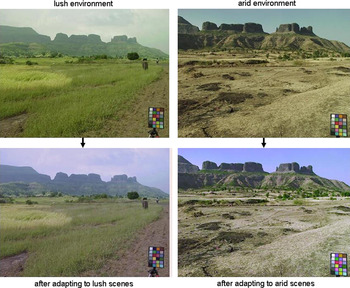
Fig. 1 illustrates an example of how color appearance changes following simulated adaptation to different environments. The upper pair of images shows roughly the same scene in India captured during the monsoon (wet) or winter (dry) seasons. In the lower images, the scene colors have been rendered after adjusting the channels so that the average channel responses within each environment are the same. Specifically, colors in the monsoon scene have been transformed by simulating how the image would appear after rescaling the sensitivities in the cones and postreceptoral processes so that within each channel, the mean response to the monsoon images equaled the mean response to the winter images, or vice versa.
(Color online) An example of images rendered to simulate adaptation to the color statistics of the environment. The top pair of images shows two similar views taken during the monsoon or winter seasons in India. In the lower pair, the colors have been adjusted after adapting the model mechanisms so that the average responses to the monsoon scenes equal the average responses to the winter scenes or vice versa.

Such images allow one to visualize how colors might appear to identical observers living in different environments (i.e., to observers with the same color mechanisms but adapted differently to each setting) (McDermott et al., Reference McDermott, Juricevic, Bebis, Webster, Rogowitz and Pappas2008). During the monsoon, the hillsides are dominated by lush green vegetation and, as we note below, chromatic contrasts tend to vary more strongly along an axis closer to the S versus LM dimension. An observer within this setting should become desensitized to these dominant color features and in particular to the average green bias in the scene so that they become toned down and less salient (lower left). Alternatively, during the arid winter season, the dominant terrestrial color shifts toward yellow and the principal axis of the color variations rotates toward the negative diagonal of the L versus M and S versus LM space, a direction that appears as a bluish-yellowish variation. Greens are now rare, and adaptation heightens their contrast and perceptual salience so that they are now highly conspicuous (lower right). In fact, these changes are consistent with anecdotal observations about changes in color perception as one travels to new locations or becomes acclimated to old ones.
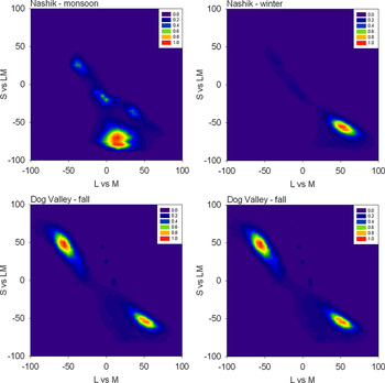
To quantify these changes, we examined the differences in the distributions and the presumed differences in adaptation states to them. Fig. 2 plots the probability distributions for chromatic contrasts from the two environments during the two seasons. In each, the density of colors has two prominent lobes corresponding to pixels from the earth and sky, and the colors tend to be biased along the negative, bluish-yellowish diagonal of the space. Across the four settings, there are changes in the mean chromaticity and in the range and direction of the principal axis of the contrast distribution. If the landmarks of color appearance reflect fixed physiological signals, then adaptation to differences in the mean chromaticity should alter the perception of the white point, while adaptation to the differences in the contrasts should alter both perceived contrast and perceived hue. We consider these in turn.
(Color online) Probability density distribution for chromaticities in the L versus M and S versus LM space from the four settings.

Average scene colors and the perception of white
In conventional models of color coding, the achromatic axis represents the null point of the color-opponent channels and thus also corresponds to the balance of activity across the cones that would give rise to this null (Hurvich & Jameson, Reference Hurvich and Jameson1957). The cones or cone-specific pathways adapt to the average color they are exposed to, and thus one basis for establishing the white point might simply be adaptation to the average color in the environment (MacLeod, Reference MacLeod, Ottoson and Zeki1985; Brainard & Wandell, Reference Brainard and Wandell1992). In that case, judgments of the stimulus that appears achromatic should vary across observers if the average color of their environment varies. As noted in the Introduction section, consistent with this we have recently found that the stimulus that appears achromatic is also the null point for chromatic adaptation, suggesting a close link between the stimulus that appears subjectively neutral and a neutral response state in visual coding (Webster & Leonard, Reference Webster and Leonard2008).
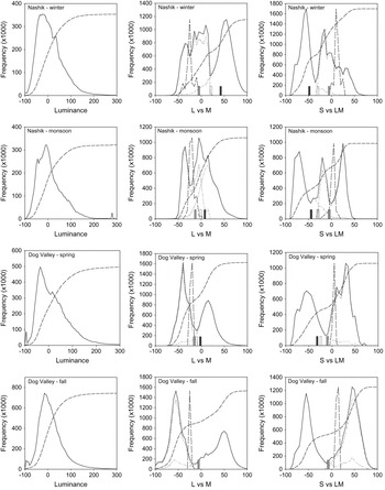
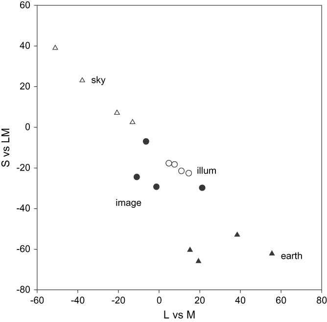
How much might this sensitivity differ because of differences in the average color of different natural contexts? To examine this, we compared the achromatic point to the mean chromaticity of the distributions. Fig. 3 plots the signals along the luminance axis and the L versus M and S versus LM opponent axes for each setting. The set of luminances is unimodal and skewed toward higher light levels, similar to previous measurements (Laughlin, Reference Laughlin1987; Ruderman & Bialek, Reference Ruderman and Bialek1994). Signals along the chromatic axes are instead markedly bimodal, again because of the color differences between sky and earth. As a result, the average chromaticity falls near the trough between these two image regions and thus is unrepresentative of most colors in the images. Brown (Reference Brown1994) noted that the average color of scenes is often not gray, but the present results suggest that even when the mean color is achromatic, grays may be relatively rare in at least some natural outdoor environments.
Histograms of the luminance, L versus M, and S versus LM contrasts for each environment. Solid lines show the distribution for all image pixels for luminance or for the two chromatic axes after equally weighting the sky and earth distributions. Dotted lines show the separate histograms for earth and sky, while medium dashed lines show the cumulative probability based on both image regions. Short dashed lines give the distribution of illuminant chromaticities, arbitrarily scaled to the same relative height. Bars for the chromatic distributions show the average L versus M or S versus LM chromaticity for the original images (black) or after weighting earth and sky equally (white) or in the ratio that provided a mean chromaticity closest to the nominal white (gray).

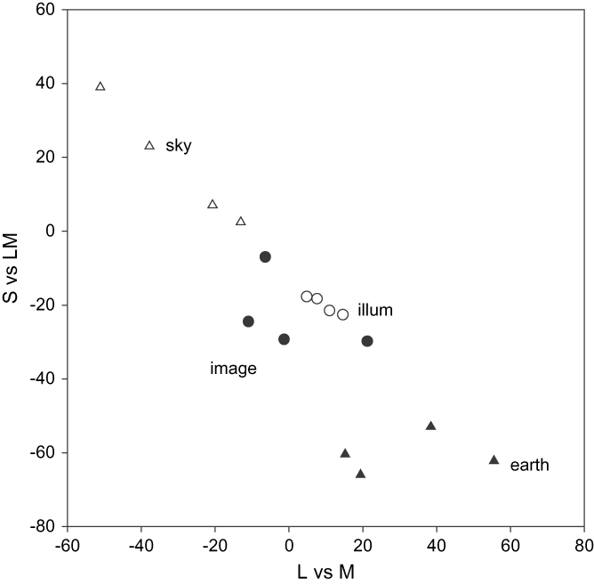
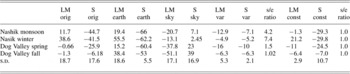
The average chromaticity differs substantially across the four contexts, and this predicts that the achromatic settings should differ both across locations and over time. However, these averages obviously depend on how the original scenes were sampled and in particular on the ratio of earth to sky in the images. We therefore tried to assess the perceptual white point in three different ways by comparing the color distributions measured separately from the earth and sky (also plotted in Fig. 3). First, it is evident that mean differences persist even when the earth and sky regions are considered in isolation. It is also clear that adaptation to the earth or sky alone could not determine the white point. The terrestrial colors are on average too green or yellow, and thus some adaptation to sky would be required to offset this bias (MacLeod & von der Twer, Reference MacLeod, von der Twer, Mausfeld and Heyer2003; Webster et al., Reference Webster, Mizokami and Webster2007). As a second way of comparing variability across the scenes, for each image set we asked what ratio of earth to sky colors would give the closest approximation to the nominal white. This is shown in Table 1 and Fig. 4. It is notable that different mixtures of earth and sky from each setting can yield a chromaticity near to white and thus similar to each other. However, this required close to an equal balance for the Sierra scenes in the fall while a sevenfold difference for the winter scenes in India. Thus, to maintain a constant adaptation-defined white balance across the different environments, observers would need to sample the images very differently. As a final approach, we instead asked what the average chromaticity would be if observers sampled earth and sky in the same proportion. This was fixed at an equal ratio (again close to the white balance implied by the fall Sierra scenes) and is the scaling shown for the earth and sky colors in Fig. 3. These comparisons still have the problem that color is not uniform within the earth and sky, and thus we cannot confidently estimate the actual variations in average color that would be expected by an observer viewing all four environments in the same way. Nevertheless, it is unlikely that this observer would remain in the same state of chromatic adaptation and thus likely that the stimulus corresponding to white should change.
Mean chromaticities for the images or illuminants (open circles) from the four different environments. Image means are shown separately for earth (filled triangles) and sky (open triangles) regions or for the equally weighted regions (filled circles).
Average scene chromaticities for the different settings

The mean L versus M and S versus LM values averaged across each image set are shown based on the entire images (orig) or on the pixels analyzed separately for earth or sky regions (earth, sky). Mean values are also shown after finding the ratio of earth and sky (s/e ratio) that yielded a chromaticity closest to the nominal white (var) for each scene, or by weighting the earth and sky equally (const).
The range of average colors across the images is at least comparable in magnitude to the observed range of individual differences in achromatic settings, which can be pronounced. However, the observed pattern for these does not clearly mimic the pattern suggested by the scene colors we analyzed. First, the differences between individuals vary primarily along directions that change from blue to yellow (Werner & Schefrin, Reference Werner and Schefrin1993; Beer et al., Reference Beer, Dinca and MacLeod2006; Webster & Leonard, Reference Webster and Leonard2008). For the environments we tested, the color changes are instead more dominant along the L versus M axis since this is the axis that captures seasonal changes in the color of vegetation. On the other hand, the average colors for sky and earth do fall roughly along this axis, and thus could, for example, vary among observers according to how they sample different image regions. Second, despite large individual differences, relatively little variability in achromatic settings has been reported for different populations (Ganz, Reference Ganz1979), while these population differences are predicted from adaptation. This discrepancy could be because we modeled natural environments, while most modern observers live in and are presumably adapted by predominantly artificially colored settings. A second possible reason is that variations in the underlying white point can only be revealed by controlling the immediate state of chromatic adaptation (e.g., by probing the stimulus that appears white during dark adaptation so that the subject is not simply normalized for the current ambient stimulus). Thus, it remains to be empirically established whether population differences occur in ways that can be related to differences in the color environment, and we note again that there is in fact currently little actual data on color appearance across environments that has controlled for the states of adaptation in ways that would allow meaningful comparisons to the effects we model.
The fact that the color distributions required for the white point are bimodal also has implications for the visual response to contrast—or differences relative to white. Models based on coding efficiency predict that the contrast response function should be shaped to equate the probability of different output levels for the expected input distribution (Laughlin, Reference Laughlin1987). For a unimodal distribution, this implies a sigmoidal contrast response that is steepest where color signals are most common and asymptotes at very low and high contrasts where signals are rare. This is shown by the dashed curve in each figure that plots the cumulative probability function. (A similar but shallower curve is predicted when response levels are equated in the presence of assumed noise; MacLeod & von der Twer, Reference MacLeod, von der Twer, Mausfeld and Heyer2003.) The observed contrast responses for luminance and color—and the fact that for both, contrast discrimination is best near the adapting gray—are consistent with these assumptions. On a finer scale, however, the different distributions for luminance and chromatic contrasts predict response functions with different shapes. In particular, sensitivity should not be highest near the white point since it is not the most frequent color in the scenes. This is at odds with psychophysical measurements which have found that luminance or chromatic contrast discrimination is indistinguishable when the stimuli are equated for multiples of detection threshold (Switkes et al., Reference Switkes, Bradley and De Valois1988). It is possible that physiological constraints prevent the visual system from matching the more complex variation in chromatic signals or that the visual response is matched to a different environment than the ones sampled here.
Scene contrasts and perceived contrast
We next examined how the perception of contrast should vary when the “same” observer is adapted to different environments. Like the variations in white, such changes are likely because the visual system readily adapts to contrast, and empirical studies have shown that subjective luminance and chromatic contrast can be strongly biased by exposure to low- or high-contrast images (McDermott et al., Reference McDermott, Sharma and Webster2007) or when contrast available to observers is reduced (Ross, Reference Ross1975; Kwon et al., Reference Kwon, Fang, Cheong, Legge and He2007). As noted in the Materials and methods section, in this case the adaptation was modeled by the gain changes in multiple postreceptoral channels formed by different linear combinations of the cone signals and thus tuned to different directions in color space. For the illustrated simulations, we used the distributions formed by equal mixtures from the earth and sky distributions, again to try to make the sampling for the different image sets comparable and consistent with plausible white points. Changes in perceived contrast were then estimated by measuring the response to each channel to a pair of distributions and then rescaling the channel sensitivities so that the average response was the same in the presence of each context.
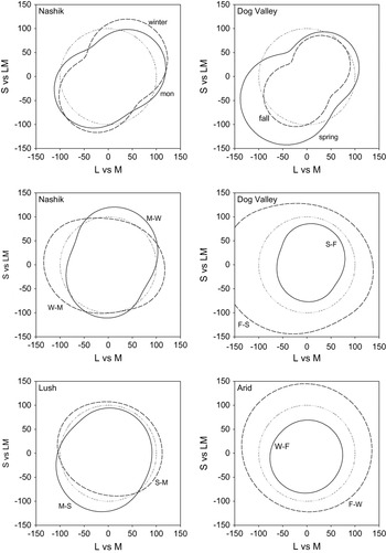
Fig. 5 shows the predicted changes in apparent contrast between different environments. In these plots, smaller values correspond to lower perceived contrast and thus reflect higher physical contrast in the images. That is, scenes with high stimulus contrast lead to stronger adaptation and thus lower apparent contrast for the same physical stimulus. The upper panels show the perceptual changes in the Nashik or Dog Valley scenes relative to a uniform color distribution with a contrast range equal to the average of the contrasts across the four measured settings. For each, the bias in the color gamuts along a bluish-yellowish direction predicts that observers should have reduced contrast sensitivity to blue-yellow variations relative to other chromatic directions. This is consistent with some studies of chromatic discrimination (Nagy et al., Reference Nagy, Eskew and Boynton1987) that have found higher thresholds along the blue-yellow direction, yet not with other work showing that contrast thresholds can be accounted for by independent signals along the two cardinal axes (Cole et al., Reference Cole, Hine and McIlhagga1993; Sankeralli & Mullen, Reference Sankeralli and Mullen1996). The predicted losses are also not clearly evident in measures of suprathreshold apparent contrast (Switkes, Reference Switkes2008).
Representations of perceived color contrast across the four different environments. Lines show the iso-contrast contours within a given environment if the model channels are adapted to give the same average response as to a reference environment. Top panels plot the response to the Nashik or Dog Valley settings when adaptation is equated for a uniform color distribution (dotted line). Middle panels show the shift in perceived contrast across seasons at the same locations. In this case, the iso-contrast lines show the response to one setting (e.g., monsoon) after adapting to equate average responses to the reference setting (e.g., winter). The reference is thus again shown by the uniform contour (dotted line). Bottom panels instead show the changes in perceived contrast across the two locations during comparable (lush or arid) seasons.

Between the environments, there are also strong predicted changes in perceived contrast since these environments differ in both the range and direction of the chromatic variations. In particular, in both locations the seasonal changes in the images predict that the perceptual salience of reddish-greenish axes would cycle inversely with the stimulus contrasts along these axes, as also illustrated in Fig. 1. On the other hand, when comparisons are made across the two locations in similar seasons (wet or dry), then the contrast changes are less selective. The specific changes again depend on how the scenes are sampled, but like the white point suggest that the perception of color contrast should vary in measurable ways across observers if perceived contrast depends on adaptation to the local environment.
Scene contrasts and perceived hue
As Fig. 5 shows, the predicted changes in contrast sensitivity are selective for the color directions that the images vary along. Because these directions change for the different environments, this predicts that an observer adapted to each setting should also experience changes in perceived hue—if these hue percepts correspond to a fixed pattern of responses as conventional color-opponent models assume. To explore these, we again compared the channel responses after adapting them to two different settings and then asked which stimulus directions would produce the same relative responses across the channels. These were defined as the stimuli that gave the same ratio of signals along the L versus M and S versus LM axes and thus the same angles in the plane defined by these axes.
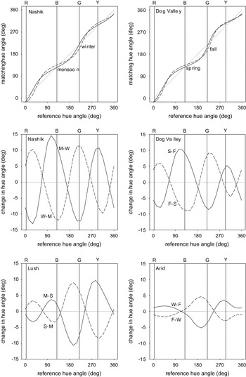
Fig. 6 plots how perceived hues should be distorted across the different settings. As before, the upper panels plot the changes relative to a uniform color distribution, while the lower panels show the biases going from one season to another or between the two locations. Losses in sensitivity along a bluish-yellowish direction bias the appearance of other stimuli away from this axis. To maintain the same neural responses, the stimulus direction must be rotated toward this axis to null out the bias. The predicted rotations relative to an unbiased color environment are up to 30° within the plane and thus perceptually large.
Changes in perceived hue across the different settings. Top panels plot the hue changes for the four environments when the responses to each are adapted to equate them to the mean responses to a uniform distribution. Lines show the chromatic angle in the adapted environment that would match the hue of a given angle in the reference environment. Middle panels plot the predicted differences in hue angles for stimuli that would match in hue after adapting to different seasons, while lower panels plot the corresponding changes across different locations.

Changing between the four environments (e.g., across seasons or across locations) results in rotations of up to 10° in the stimuli that would be chosen as the unique hues. While this difference is perceptually distinguishable, it is smaller than the range of individual differences that have been reported for the unique hues (Webster et al., Reference Webster, Miyahara, Malkoc and Raker2000; Kuehni, Reference Kuehni2004). Importantly, it is also generally too small to shift the perceived color category or label for the stimulus. That is, adaptation to the different distributions is likely to alter the perceived shade of red but not strong enough to cause the same stimulus to be labeled with a different color term like orange or purple. Within-category color differences of this kind were observed by Webster et al. (Reference Webster, Webster, Bharadwadj, Verma, Jaikumar, Madan and Vaithilingam2002) who compared unique hues across observers in India and the United States. While these different populations chose very similar points in color space for a given focal color (relative to the distances between different colors), there were nevertheless significant differences in the mean focal stimulus within most categories. A similar pattern was found by Webster and Kay (Reference Webster, Kay, MacLaury, Paramei and Dedrick2007) in a study of population differences in focal colors based on the World Color Survey. When projected as angles into the color space used in the current study, the mean focal colors from different populations have a standard deviation of 1.4 deg for red and between 4° and 5° for blue, green, and yellow. The overall range of variation in focal choices across the different language groups is comparable in magnitude to the range predicted from natural seasonal variations in our model. Thus, both the observed differences in color naming and the differences predicted by adaptation largely reflect modulations in appearance within rather than between color categories. However, as noted in these studies, one discrepancy is that the hue rotations induced by contrast adaptation should lead to correlated variations across the different hues, while the observed variations in unique hues both between individuals and between different linguistic groups are independent.
Spatial variations in color statistics
Thus far, we have considered how color appearance should change when observers are exposed to different environments. However, the color statistics within an environment are not stationary. For example, the differences between sky and earth that were noted above apply to different locations in the images. To the extent that adaptation is local, this suggests that different regions of the retina may be adapted in different ways. In fact, it is likely that local adaptation underlies the compensation for spatial variations in visual sensitivity, for example, compensating the white point for the fall off in macular pigment with eccentricity (Beer et al., Reference Beer, Wortman, Horwitz and MacLeod2005; Webster & Leonard). In this case, adaptation maintains perceptual constancy by discounting changes in the observer. However, the same processes should lead to changes in color appearance within the observer if the environment itself changes across the visual field.
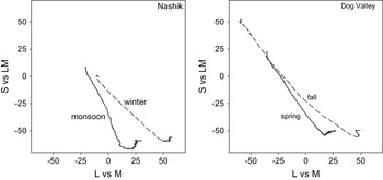
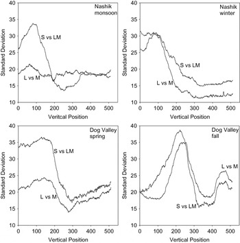
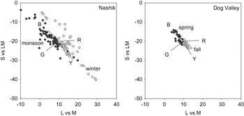
Figs. 7 and 8 show the average chromaticities and standard deviations of chromatic contrasts for different vertical locations in the image sets. Averaged across the individual images, the mean color varies systematically along the bluish to yellowish-green direction of the sky and earth and is similar in pattern across the different image sets. An observer scanning such scenes will on average be exposed to more blue on the lower retina and more yellow-green on the upper retina and consequently should have predictably different achromatic settings for the upper and lower fields. The spatial variations in chromatic contrast are less consistent across the settings but are higher in the central and upper regions of the image, presumably because these areas are more likely to alternate between sky and earth. Again these results depend on how the original images sampled the environment and not necessarily on how an actual observer might. However, they once more suggest that local adaptation to the differences across the images should lead to differences in the perceived hue and contrast of the same stimulus in the upper and lower visual fields. We are not aware of studies that have directly assessed this, but measurements of this kind might provide a further potential test of models in which color appearance depends on special response states in mechanisms that adapt to their local context.
Variations in mean chromaticity within environments. Curves show the average chromaticity at different vertical positions in the images from each setting and vary from bluish to yellow-green for each setting as pixel location varies from top to bottom.

Variations in contrast within environments. Lines plot the standard deviation in the L versus M or S versus LM contrast as a function of the vertical position from the top (0) to bottom (512) of the images from each setting.

Color appearance and the illuminant
In the preceding analyses, we focused on the color signals in the scenes and examined how adaptation to these would be expected to alter the perception of color if appearance is based on fixed physiological rules such as the null points of color-opponent channels. As we noted in the Introduction section, an alternative to such models is that the perceived color depends on specific color properties of the environment. In that case, the responses corresponding to a particular hue could obviously vary if the signal for that hue did not covary with the color signals controlling the adaptation.
One proposed candidate for a salient color feature in the environment is the color of the illuminant (Pokorny & Smith, Reference Pokorny and Smith1987; Lee, Reference Lee1990; Shepard, Reference Shepard, Barkow, Cosmides and Tooby1992; Mollon, Reference Mollon2006). We therefore also examined how the illumination varied across the different contexts. The ambient illumination in each of the images was measured when the images were originally captured by recording the light spectrum reflected from the white chip on the Munsell reference palette (Webster et al., Reference Webster, Mizokami and Webster2007). The illuminant chromaticities are shown in both Fig. 3 and Fig. 9. Compared to the average scene color, the average illumination varied less across the four conditions (see Figs. 3 and 4). Thus, most of the change in the color distributions was due to changes in objects (e.g., vegetation) or media (e.g., sky) rather than the lighting. Moreover, these averages also remained closer to the nominal white (though biased toward yellow) and were confined more clearly to a blue-yellow direction. Consequently, if the white point were based on the average illuminant color—rather than the average scene color—it should remain more stable across environments and might be expected to vary across individuals more tightly along the blue-yellow dimension, as actual measurements suggest.
Variation in scene illuminants. Points plot the chromaticities of the illumination measured for individual scenes in the four different environments. Lines show estimates of the directions corresponding to unique blue, yellow, red, or green from Webster et al. (Reference Webster, Miyahara, Malkoc and Raker2000).

Variations in the individual illuminants were also clustered along a blue-yellow direction. As several authors have noted previously, this could provide the potential signal for defining unique blue and yellow (Pokorny & Smith, Reference Pokorny and Smith1987; Lee, Reference Lee1990; Shepard, Reference Shepard, Barkow, Cosmides and Tooby1992; Mollon, Reference Mollon2006). This is shown in Fig. 9, where the spread of illuminant colors is compared to the directions of the four unique hues based on the study of Webster et al. (Reference Webster, Miyahara, Malkoc and Raker2000). The variations in daylight are reasonably concordant with the perceptual blue-yellow loci, especially given that the yellow settings of Webster et al. had a somewhat lower dominant wavelength compared to other estimates, and as noted individual differences in the unique hues are large. Thus, we cannot exclude a model of color appearance based on learned properties like the illuminant. Studies of color constancy have often emphasized the importance of factoring out the illumination in order to reliably represent an object’s color. Yet, it is intriguing that it is variations in the illuminant that could underlie some fundamental dimensions of color appearance.
Conclusions
Color coding is intrinsically adaptable and thus should change depending on the world the observer is adapted to. Here we have modeled how color appearance should vary because of adaptation to different natural color environments, if we assume no variation in the underlying neural coding in the observer. The actual changes depend on a number of factors including the assumed properties of the stimulus (e.g., the color statistics of the environment and how these are sampled in natural viewing) and the observer (e.g., the number and selectivity of the adapted channels and the nature of the sensitivity changes). Thus, at best our results are only illustrative of the types of changes that might occur and more specifically of the changes that could occur for the particular natural outdoor environments we examined. Whether this approach might predict actual measures of color appearance in different observers or populations awaits better knowledge of the color statistics of modern environments and better control of the states of adaptation during testing. Nevertheless, these results point to the general form and magnitude of individual and population differences in perceptual judgments of color that might result from differences induced by adaptation to specific environments. In particular, they illustrate that models of color appearance based on fixed weightings of the cone signals actually imply substantial variation in color vision because the color signals that produce these fixed weightings vary with the state of adaptation, and the states of adaptation are likely to vary substantially in different natural visual environments. Transforming images to embody these sensitivity changes provides a novel approach for exploring the consequences of long-term adaptation on color appearance and, as illustrated in Fig. 1, provides a tool for simulating how the world might look to others.
Acknowledgments
Supported by EY-10834.