1 Introduction
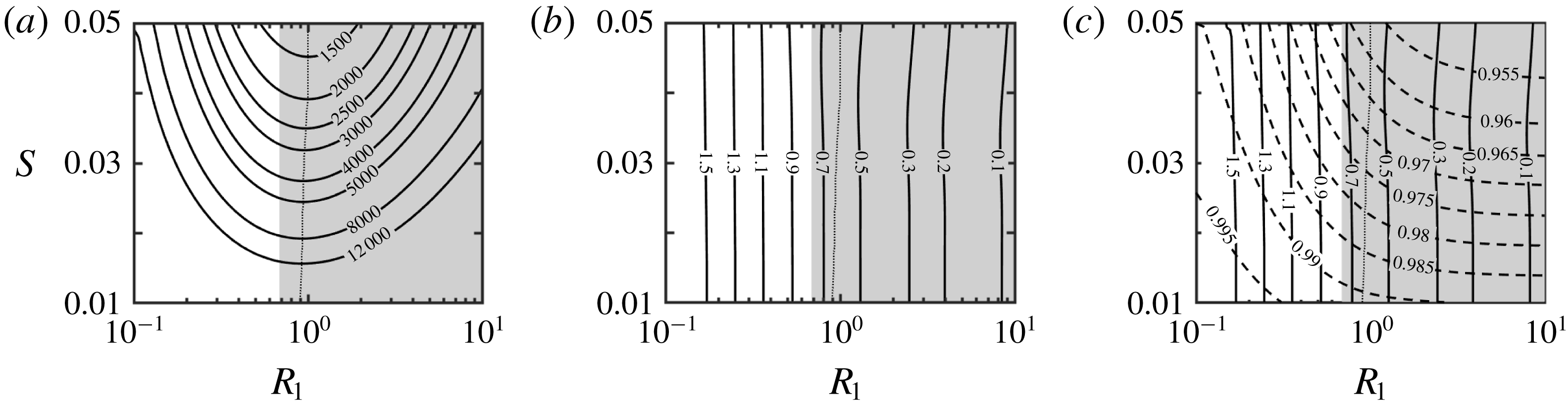
Annular conduits are frequently used in petroleum engineering, heat exchangers, turbomachinery, fuel cells, aero-engines and various chemical industrial devices, among many others. The efficiencies of these devices depend on the flow characteristics. The properties of such flows in the case of smooth concentric cylinders are well known (Joseph Reference Joseph1976). Our interest is in the development of passive flow rearrangement strategies relying on surface topographies that would lead to better flow properties than in the unmodified annuli. Two criteria assisting with the determination of what ‘better’ means will be used, i.e. (i) reduction of the pressure drop required to create a desired flow rate in the modified annuli as compared with the unmodified annuli, and (ii) the ability to create secondary flows which would lead to mixing enhancement. In the latter case, we shall focus attention on the use of natural instabilities for the creation of such flows, as this would result in a smaller cost expressed in terms of pressure losses. We shall limit this analysis to small-amplitude longitudinal grooves and determine what flow changes can be achieved through their judicious deployment. The small-amplitude limitation is introduced intentionally so that we can focus on changes of surface topography rather than changes in the overall duct shape. Since it is known that axisymmetric grooves (ribs) always increase drag (Mohammadi & Floryan Reference Mohammadi and Floryan2012, Reference Mohammadi and Floryan2013b ; Moradi & Floryan Reference Moradi and Floryan2017b ), this class of topographies will not be further considered.
There are two elements to the question of drag reduction. The first element deals directly with drag reduction and involves the determination of surface topographies that could achieve this objective without changing the mean annulus opening. Grooves, obviously, can be viewed as a form of distributed roughness. It is known that grooves parallel to the flow direction result in a reduction of friction in the case of turbulent flows (Walsh Reference Walsh1983) but these grooves, which are referred to as riblets, have excessively short wavelengths and suffer from contamination, resulting in their clogging as well as destruction when exposed to shear for extended periods of time. It has been shown recently that such grooves can either destabilize the flow or play a neutral role depending on their orientation with respect to the main stream direction (Ho & Asai Reference Ho and Asai2018). A different class of drag-reducing grooves with longer wavelengths was developed and extensively studied in the case of laminar (Mohammadi & Floryan Reference Mohammadi and Floryan2013a ; Moradi & Floryan Reference Moradi and Floryan2013b ) as well as turbulent (Chen et al. Reference Chen, Floryan, Chew and Khoo2016; DeGroot, Wang & Floryan Reference DeGroot, Wang and Floryan2016) channel flows. Similar grooves are known to reduce the laminar frictional drag in annular flows (Moradi & Floryan Reference Moradi and Floryan2013a ). The drag-reducing effect is associated with the formation of high-velocity stream tubes in the widest opening of the conduit. The limits of applicability of these grooves are not known, as the resulting flows may exhibit a range of instabilities that could affect their drag-reducing capabilities, and the stability characteristics of such flows are yet to be studied.
The second element of the drag reduction problem is related to the laminar–turbulent transition and determination of conditions that could either prevent or delay this process. As the laminar flows generate significantly smaller frictional drag than turbulent flows, there is an interest in determination of conditions which guarantee their existence. This question is very prominent in the aerospace industry, where the focus is on the development of natural laminar-flow airfoils (Arnal, Perraud & Seraudie Reference Arnal, Perraud and Seraudie2008) but is less common in the analysis of internal flows. It is known that the transition process in smooth annuli begins in the case of a quiet environment with the shear-driven instability resulting in the formation of Tollmien–Schlichting (TS) waves (Mott & Joseph Reference Mott and Joseph1968; Mahadevan & Lilley Reference Mahadevan and Lilley1977; Garg Reference Garg1980; Heaton Reference Heaton2008). The character of these waves depends on the annuli’s radii, as annuli with larger radii give preference to axisymmetric waves while annuli with smaller radii promote various forms of spiral waves. The important role of the finite-amplitude disturbances was documented by Shapiro, Shtilman & Tumin (Reference Shapiro, Shtilman and Tumin1999), but detailed explorations of transitional structures are very recent (Ishida, Duguet & Tsukahara Reference Ishida, Duguet and Tsukahara2016). Various bypass processes are possible, but they are yet to be explored. It is known that, in the case of channel flows, transverse grooves can convert transient growth into asymptotic growth, thus guaranteeing transition to a new state (Szumbarski & Floryan Reference Szumbarski and Floryan2006). Phenomenological estimates of the critical Reynolds number are well summarized by Dou, Khoo & Tsai (Reference Dou, Khoo and Tsai2010).
It is generally believed that surface roughness accelerates transition, i.e. the critical Reynolds number for rough surfaces is smaller than for smooth surfaces. Grooves can be viewed as a class of distributed surface roughness and one could presume that they always decrease the critical Reynolds number. This, however, may not be the case for the drag-reducing topographies, as they reduce viscous friction, and this may stabilize the shear-driven TS waves. The same grooves create spatial flow modulations which may activate instability mechanisms not operational in the case of smooth surfaces, but which may reduce the critical Reynolds number below that found for the TS waves. It is rather impossible to predict how grooves may affect flow properties without carrying out a detailed analysis, as their different distributions may increase or decrease the critical Reynolds number. It is known that, in the case of channel flows, individual grooves may have no effect on the stability properties but can reduce the critical Reynolds number when forming certain patterns (Floryan & Asai Reference Floryan and Asai2011). The related question to be addressed is the flow sensitivity to the presence of grooves (or the presence of roughness). One is interested in the determination of when the roughness can be ignored, and the walls can be viewed as being hydraulically smooth, and when the roughness is hydraulically active and must be accounted for. It should be stressed that the frequently used definition of hydraulic smoothness, based on whether a roughness element extends outside the laminar sublayer, does not apply to laminar flows and an alternative definition of hydraulic smoothness is required (Floryan Reference Floryan2007).
The question of mixing intensification is directly related to the question of transport of scalar quantities across the annuli, e.g. heat transfer, which relies in the case of laminar flows on diffusion only. The creation of transverse fluid movement can intensify this process by several orders of magnitude, and different methods for achieving this goal were investigated (Webb & Bergles Reference Webb and Bergles1983). The first group of techniques relies on a purely mechanical mixing associated with the use of vortex generators and is very effective but carries a large pressure drag penalty (Jacobi & Shah Reference Jacobi and Shah1995; Fiebig Reference Fiebig1995a ,Reference Fiebig b , Reference Fiebig1998). The second group relies on the promotion of the laminar–turbulent transition under subcritical conditions (Fiebig & Chen Reference Fiebig, Chen, Kakac, Bergles, Mayinger and Yuncu1999) as turbulent mixing is very effective. The third group of methods relies on the use of flow modifications to create chaotic advection (Aref Reference Aref1984; Stroock et al. Reference Stroock, Dertinger, Ajdari, Mezic, Stone and Whitesides2002; Sturman, Ottino & Wiggins Reference Sturman, Ottino and Wiggins2006). The fourth group relies on mechanical mixing induced by wall vibrations (Selverov & Stone Reference Selverov and Stone2001; Carlsson, Sen & Löfdahl Reference Carlsson, Sen and Löfdahl2005; Jiménez-Lozano, Sen & Dunn Reference Jiménez-Lozano, Sen and Dunn2009). The focus of this analysis is on the fifth group of methods, i.e. those which rely on the creation of secondary flows. Judicious deployment of grooves may result in the creation of such flows, which could provide the desired transverse fluid movement. Such secondary flows could also provide means for acceleration of the laminar–turbulent transition if this is what is desired. The use of transverse grooves for creation of streamwise vortices through centrifugal effects was studied for channel flows (Floryan Reference Floryan2003, Reference Floryan2015; Gepner & Floryan Reference Gepner and Floryan2016; Moradi, Budiman & Floryan Reference Moradi, Budiman and Floryan2017). While the centrifugal effect is not available in the case of longitudinal grooves, it is known that they can create a new class of travelling waves in channel flows (Moradi & Floryan Reference Moradi and Floryan2014; Mohammadi, Moradi & Floryan Reference Mohammadi, Moradi and Floryan2015; Yadav, Gepner & Szumbarski Reference Yadav, Gepner and Szumbarski2017), so the conditions leading to the formation of such waves in annular flows as well as their properties are of interest. One of the questions to be addressed is the competition between such waves and the TS waves and determination if the new waves offer any advantages over the TS waves.
The above discussion shows that grooves can be used to achieve a variety of mutually exclusive objectives. They can be viewed as drag-reducing devices; in this case, one is interested in the determination of flow conditions that limit their applicability. They can be viewed as means for creation of secondary flows; in this case, one is interested in the selection of grooves that promote the desired classes of secondary flows. They can be viewed as a form of surface roughness; in this case, one is interested in the determination of flow sensitivity to their presence. In all cases, grooves can be viewed as passive flow control devices and knowledge of flow response to their presence is essential for their effective utilization. This analysis is focused on the determination of flow responses to the presence of such grooves, with the resulting knowledge providing a basis for selection of their shape and distributions to meet the specific objectives of interest to the potential user.
This paper is organized as follows. Section 2 provides a description of primary flows in the groove–modified annuli. Section 3 presents the problem formulation required for the determination of secondary flows. Section 4 provides a description of such flows. Section 4.1 summarizes what is known about such flows in smooth annuli. Section 4.2 discusses the properties of TS waves and how they are changed by the grooves. Section 4.3 describes new waves created by the grooves. Section 4.4 provides a discussion of the instability mechanism at play in such flows. Section 4.5 discusses the domains of attraction of different secondary flows and the competition between such flows. Section 4.6 is focused on the question of hydraulic smoothness. Section 4.7 addresses the question of the effects of groove shapes. Section 5 provides a short summary of the main conclusions.
2 Mean flow
2.1 Problem formulation
Consider steady flow in an annulus extending to
 $\pm \infty$
in the axial direction and formed by a smooth outer cylinder and an inner cylinder equipped with
 $M$
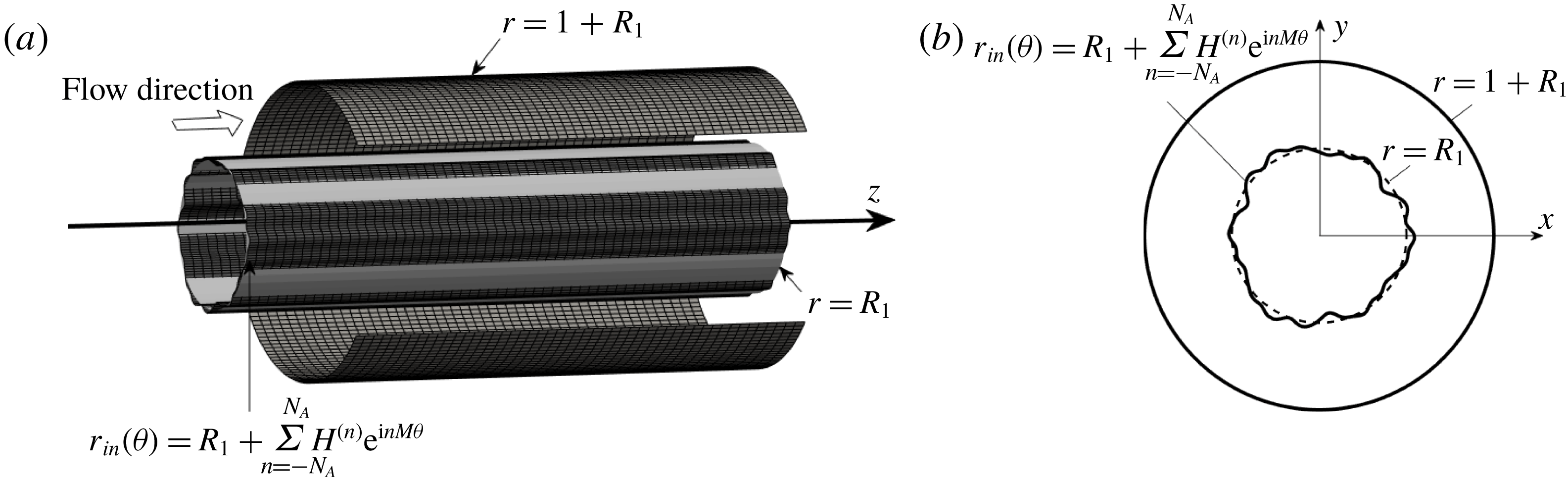
identical longitudinal grooves. The conduit geometry is illustrated in figure 1 and is described as
 $$\begin{eqnarray}r_{in}(\unicode[STIX]{x1D703})=R_{1}+\mathop{\sum }_{n=-N_{A}}^{N_{A}}H^{(n)}\text{e}^{\text{i}nM\unicode[STIX]{x1D703}},\quad r_{out}=1+R_{1},\end{eqnarray}$$
where subscripts ‘
 $in$
’ and ‘
 $out$
’ denote the inner and outer cylinders, respectively,
 $N_{A}$
is the number of Fourier modes required to describe the groove geometry,
 $H^{(n)}=H^{(-n)\ast }$
are the reality conditions, with star denoting the complex conjugate,
 $R_{1}$
stands for the radius of the inner cylinder and the annulus opening
 $L$
is used as the length scale. Since groove amplitude is small, changes in the cylinder geometry should be viewed as variations of surface topography rather than as changes in the overall conduit shape.
The flow is unidirectional and is driven by a constant axial pressure gradient. The axial momentum equation serves as the governing equation along with the no-slip condition at the inner and outer cylinders as the boundary condition, i.e.
 $$\begin{eqnarray}\displaystyle & \displaystyle \frac{1}{r}\frac{\unicode[STIX]{x2202}u_{zB}}{\unicode[STIX]{x2202}r}+\frac{\unicode[STIX]{x2202}^{2}u_{zB}}{\unicode[STIX]{x2202}r^{2}}+\frac{1}{r^{2}}\frac{\unicode[STIX]{x2202}^{2}u_{zB}}{\unicode[STIX]{x2202}\unicode[STIX]{x1D703}^{2}}=Re\frac{\text{d}p_{B}}{\text{d}z}, & \displaystyle\end{eqnarray}$$
 $$\begin{eqnarray}\displaystyle & \displaystyle u_{zB}[r_{in}(\unicode[STIX]{x1D703}),\unicode[STIX]{x1D703}]=u_{zB}(r_{out},\unicode[STIX]{x1D703})=0. & \displaystyle\end{eqnarray}$$
Here we have used the subscript
 $B$
to denote this flow as the base flow for the stability analysis to be carried out in § 3, the velocity vector with components in the
 $(r,\unicode[STIX]{x1D703},z)$
directions is represented as
 $\boldsymbol{u}_{B}=(u_{rB},r_{\unicode[STIX]{x1D703}B},u_{zB})$
and
 $p_{B}$
stands for the pressure. The solution is represented as the sum of the flow in a smooth annulus, denoted by subscript 0, and the groove-induced modifications, identified using subscript 1, i.e.
 $$\begin{eqnarray}u_{zB}(r,\unicode[STIX]{x1D703})=u_{z0}(r)+u_{z1}(r,\unicode[STIX]{x1D703}),\quad p_{B}(z)=p_{0}(z)+p_{1}(z).\end{eqnarray}$$
Flow in the smooth annulus is referred to as annular Poiseuille flow (APF) (Joseph Reference Joseph1976) and its form is determined analytically, i.e.
 $$\begin{eqnarray}\left.\begin{array}{@{}c@{}}\displaystyle \boldsymbol{u}_{0}(r)=[u_{r0},u_{\unicode[STIX]{x1D703}0},u_{z0}(r)]=\left\{0,~0,~\frac{R_{1}^{2}}{k_{1}}\left[1-\left(\frac{r}{R_{1}}\right)^{2}\right]+\frac{k_{2}}{k_{1}}\ln \frac{r}{R_{1}}\right\},\\ \displaystyle \unicode[STIX]{x1D74E}_{0}=[\unicode[STIX]{x1D702}_{0},\unicode[STIX]{x1D719}_{0}(r),\unicode[STIX]{x1D709}_{0}]=\left[0,~\frac{1}{k_{1}}\left(2r-\frac{k_{2}}{r}\right),~0\right],\quad \frac{\text{d}p_{0}}{\text{d}z}=\frac{-4}{k_{1}Re},\\ \displaystyle Q_{0}=\frac{\unicode[STIX]{x03C0}}{2k_{1}}\left[-(1+2R_{1})(1+2R_{1}+k_{2})+2k_{2}(1+R_{1})^{2}\ln \left(\frac{1+R_{1}}{R_{1}}\right)\right],\end{array}\right\}\end{eqnarray}$$
where
 $k_{1}=R_{1}^{2}-k_{2}\ln R_{1}+(k_{2}/2)[\ln (k_{2}/2)-1]$
,
 $k_{2}=(1+2R_{1})/\!\ln [(1+R_{1})/R_{1}]$
,
 $\unicode[STIX]{x1D74E}_{0}$
denotes the vorticity vector and
 $Q_{0}$
stands for the flow rate. The maximum of
 $u_{z0}$
, i.e.
 $U_{max}$
, is used as the velocity scale,
 $\unicode[STIX]{x1D70C}U_{max}^{2}$
is used as the pressure scale,
 $\unicode[STIX]{x1D70C}$
stands for the density and the Reynolds number is defined as
 $Re=U_{max}L/\unicode[STIX]{x1D708}$
, where
 $\unicode[STIX]{x1D708}$
denotes the kinematic viscosity.
Sketch of the flow problem. Light grey colour in panel (a) identifies the position of the reference smooth inner cylinder. (b) The cross-section of the grooved annulus.

The problem for the flow modifications has the form
 $$\begin{eqnarray}\frac{1}{r}\frac{\unicode[STIX]{x2202}u_{z1}}{\unicode[STIX]{x2202}r}+\frac{\unicode[STIX]{x2202}^{2}u_{z1}}{\unicode[STIX]{x2202}r^{2}}+\frac{1}{r^{2}}\frac{\unicode[STIX]{x2202}^{2}u_{z1}}{\unicode[STIX]{x2202}\unicode[STIX]{x1D703}^{2}}=Re\frac{\text{d}p_{1}}{\text{d}z},\end{eqnarray}$$
 $$\begin{eqnarray}u_{z1}[r_{in}(\unicode[STIX]{x1D703}),\unicode[STIX]{x1D703}]=-u_{z0}[r_{in}(\unicode[STIX]{x1D703}),\unicode[STIX]{x1D703}],\quad u_{z1}(r_{out},\unicode[STIX]{x1D703})=-u_{z0}(r_{out},\unicode[STIX]{x1D703}),\end{eqnarray}$$
and its solution is parametrized by the modification pressure gradient
 $\text{d}p_{1}/\text{d}z$
. This modification is not known in the present analysis and, accordingly, a closing condition in the form of a fixed flow-rate constraint is added. This condition, which has the form
 $$\begin{eqnarray}0=M\int _{0}^{2\unicode[STIX]{x03C0}/M}\!\int _{r_{in}(\unicode[STIX]{x1D703})}^{r_{out}}ru_{z1}(r,\unicode[STIX]{x1D703})\,\text{d}r\,\text{d}\unicode[STIX]{x1D703},\end{eqnarray}$$
states that the flow rates in the grooved and smooth annuli are the same. Groove topologies resulting in a positive
 $\text{d}p_{1}/\text{d}z$
are of special interest, as they lead to the reduction of pressure losses.
The Fourier–Chebyshev spectral method was used to solve (2.6)–(2.8). Since boundaries are periodic in the
 $\unicode[STIX]{x1D703}$
-direction, the solution was represented as
 $$\begin{eqnarray}u_{z1}(r,\unicode[STIX]{x1D703})=\mathop{\sum }_{n=-\infty }^{\infty }f^{(n)}(r)\text{e}^{\text{i}nM\unicode[STIX]{x1D703}}\approx \mathop{\sum }_{n=-N_{M}}^{N_{M}}f^{(n)}(r)\text{e}^{\text{i}nM\unicode[STIX]{x1D703}},\end{eqnarray}$$
where
 $f^{(n)}=f^{(-n)\ast }$
expresses the reality condition and
 $N_{M}$
denotes the number of Fourier modes used in the computations. The unknown modal functions were represented in terms of the Chebyshev expansions, i.e.
 $f^{(n)}(r)\approx \sum _{k=0}^{N_{T}}G_{k}^{(n)}T_{k}(r)$
, where
 $G_{k}^{(n)}$
represent the unknown coefficients,
 $T_{k}(r)$
are Chebyshev polynomials of the first kind, and
 $N_{T}$
denotes the number of polynomials used in the computations. The Galerkin projection was used to form a system of linear algebraic equations. Boundary condition at the corrugated cylinder were enforced using the immersed boundary conditions (IBC) method (Szumbarski & Floryan Reference Szumbarski and Floryan1999; Husain & Floryan Reference Husain and Floryan2008; Moradi & Floryan Reference Moradi and Floryan2012, Reference Moradi and Floryan2017a
). The IBC method relies on the immersion of an irregular physical domain inside a rectangular computational box and the enforcement of the boundary conditions through the imposition of boundary constraints. Rows corresponding to the highest Chebyshev polynomials were replaced with the discretized form of these constraints, i.e. tau method (Canuto et al.
Reference Canuto, Hussaini, Quarternoi and Zang2006). The discretized flow-rate constraint was added to the matrix as a separate row to close the system of equations. The solution of this system results in the determination of the Chebyshev coefficients, i.e.
 $G_{k}^{(n)}$
, and the pressure gradient correction
 $\text{d}p_{1}/\text{d}z$
. Domain transformation (DT), which relies on an analytic mapping of the complex geometry onto a regular computation strip, represents an alternative method suitable for boundaries with irregularities (Cabal, Szumbarski & Floryan Reference Cabal, Szumbarski and Floryan2001; Moradi & Floryan Reference Moradi and Floryan2013a
). In this study, the IBC method was used for most computations due to its efficiency, while the DT method was used for spot checks. The IBC method can be improved using the over-constrained formulation (Husain, Szumbarski & Floryan Reference Husain, Szumbarski and Floryan2009), but this was found not to be required in the present case.
We shall use grooves with a simple sinusoidal form to discuss flow properties, i.e.
 $$\begin{eqnarray}r_{in}(\unicode[STIX]{x1D703})=R_{1}+S\cos (M\unicode[STIX]{x1D703}),\quad r_{out}=1+R_{1},\end{eqnarray}$$
where
 $S$
denotes the groove amplitude. The groove wavelength is defined as
 $\unicode[STIX]{x1D706}_{\unicode[STIX]{x1D703}}=2\unicode[STIX]{x03C0}R_{1}/M$
, and
 $M/R_{1}$
can be considered as being the effective wavenumber when making analogies with the two-dimensional channel flow. Grooves increase the wetted surface area and change the cross-sectional area of the inner cylinder. Flow modifications associated with the latter effect need to be eliminated to make valid conclusions regarding drag increase or decrease. The difference between the cross-sectional area of the grooved and smooth inner cylinders is
 $\unicode[STIX]{x03C0}S^{2}/2$
. The increase of the cross-sectional area of the grooved cylinder can be compensated by changing its average position through the introduction of a correction factor,
 $R_{cor}$
. Thus, the geometry of the inner cylinder, which has the same cross-sectional area as the reference smooth cylinder, is expressed as
 $$\begin{eqnarray}r_{in}(\unicode[STIX]{x1D703})=R_{1}+R_{cor}+S\cos (M\unicode[STIX]{x1D703}),\end{eqnarray}$$
where the correction factor is
 $R_{cor}=-R_{1}+\sqrt{R_{1}^{2}-S^{2}/2}$
.
The addition of grooves changes the distribution of the wall friction and, consequently, the pressure losses. The modification pressure gradient,
 $\text{d}p_{1}/\text{d}z$
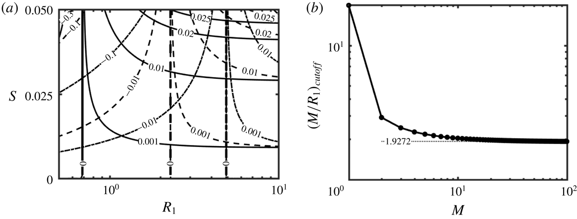
, provides a quantitative measure of drag changes. Figure 2(a) displays variations of
 $Re\,\text{d}p_{1}/\text{d}z$
as a function of the radius of the inner cylinder
 $R_{1}$
and the groove amplitude
 $S$
for three different sets of grooves (three values of
 $M$
). It can be shown that
 $Re\,\text{d}p_{1}/\text{d}z$
changes proportionally to
 $S^{2}$
and reaches the limiting value of
 $$\begin{eqnarray}Re\,\frac{\text{d}p_{1}}{\text{d}z}=-\frac{8}{1+3S^{2}/8}-\frac{3S^{2}(1+S^{2}/16)}{2R_{1}(1+3S^{2}/8)^{2}}+\frac{4}{k_{1}}+O(R_{1}^{-2}),\end{eqnarray}$$
for
 $R_{1}\gtrsim 10$
, which is the same as the pressure gradient correction in a two-dimensional channel. Data displayed in figure 2(a) demonstrate that, for each set of grooves (each
 $M$
), there exists a cutoff radius
 $R_{1,cutoff}$
which leads to the change of sign of
 $Re\,\text{d}p_{1}/\text{d}z$
, with grooves reducing drag for
 $R_{1}>R_{1,cutoff}$
. The
 $R_{1,cutoff}$
value depends marginally on
 $S$
but changes with
 $M$
as illustrated in figure 2(a).
(a) Variations of the pressure gradient corrections
 $Re\,\text{d}p_{1}/\text{d}z$
in an annulus described by (2.11) as a function of its radius
 $R_{1}$
and the groove amplitude
 $S$
. The solid, dashed and dash-dotted lines correspond to annuli with
 $M=2$
, 5 and 10 grooves, respectively, with
 $R_{1,cutoff}=0.688$
, 2.292 and 4.912 in each case, respectively. (b) Variations of the cutoff groove wavenumber
 $(M/R_{1})_{cutoff}$
as a function of the number of grooves,
 $M$
, for an annulus described by (2.11) with
 $S=0.025$
.

Figure 2(b) illustrates variations of the cutoff groove wavenumber, i.e. the ratio of
 $M$
to
 $R_{1,cutoff}$
, as a function of the number of grooves
 $M$
. Drag decreases when
 $M/R_{1}<(M/R_{1})_{cutoff}$
. It can be seen that
 $(M/R_{1})_{cutoff}$
changes from
 ${\sim}20$
for
 $M=1$
to
 $1.9272$
for
 $M\rightarrow \infty$
which, in this limit, is the same as for a plane channel if one accounts for scaling differences (Mohammadi & Floryan Reference Mohammadi and Floryan2013b
; Moradi & Floryan Reference Moradi and Floryan2013b
). Curve fitting shows that variations of
 $(M/R_{1})_{cutoff}$
can be approximated as
 $(M/R_{1})_{cutoff}=(1.9272M-0.7363)/(M-0.9187)$
. The drag reduction for
 $M/R_{1}<(M/R_{1})_{cutoff}$
is attributed to the rearrangement of the flow field (Mohammadi & Floryan Reference Mohammadi and Floryan2013b
; Moradi & Floryan Reference Moradi and Floryan2013a
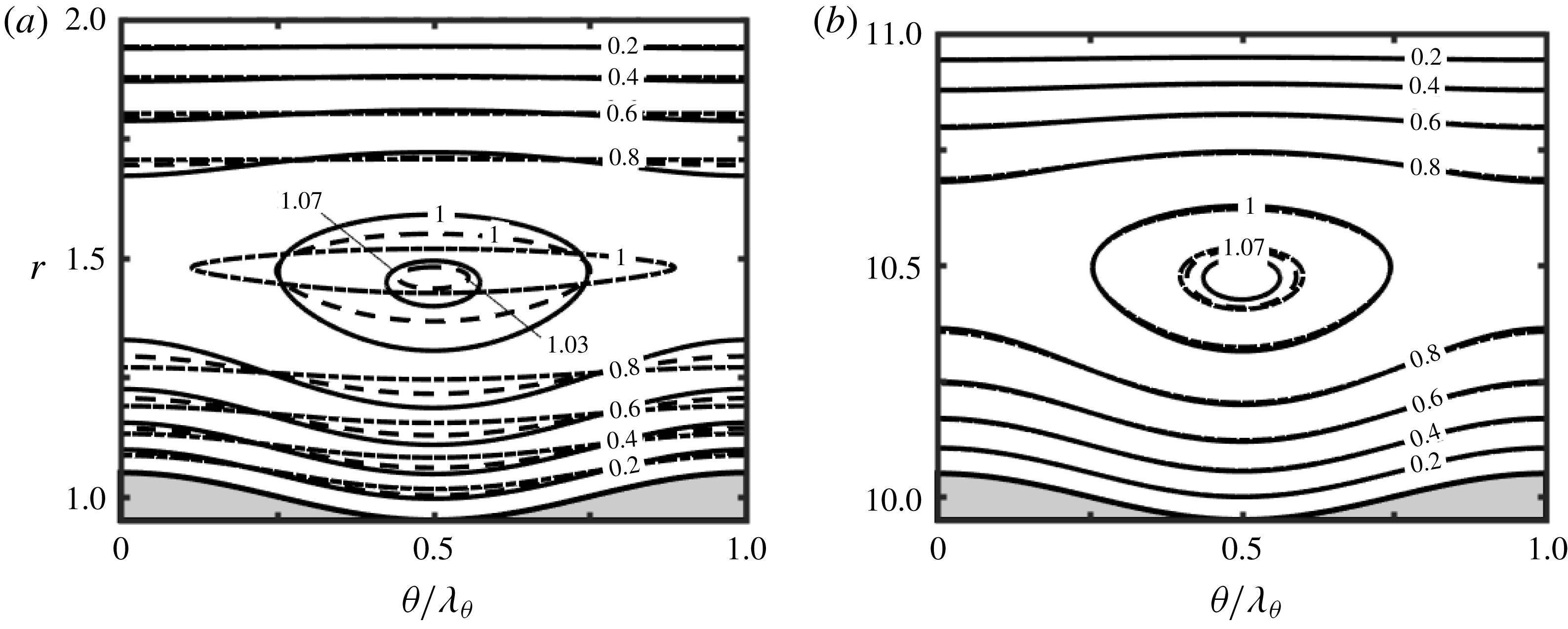
) leading to the formation of high-velocity stream tubes in the widest annulus opening, as illustrated in figure 3. This form of the flow field changes the cross-distribution of shear, which is expected to affect the TS instability and, at the same time, it introduces inflection points in the circumferential velocity distribution which may generate an inviscid instability driven by vorticity dynamics. The analysis described in the next section demonstrates that a new instability does occur.
Spatial distribution of the axial velocity
 $u_{zB}$
in annuli described by (2.11) with
 $S=0.05$
and (a)
 $R_{1}=1$
and (b)
 $R_{1}=10$
. The solid, dashed and dash-dotted lines represent results for groove numbers
 $M=2$
, 5 and 10, respectively.

3 Linear stability analysis
It is known that a secondary flow in the form of travelling TS waves appears in the APF. While the grooves are expected to change the onset conditions for these waves, they may also create a different instability due to the formation of inflection points in the circumferential direction. The onset conditions for the TS waves as well as for any new instability were determined using the linear stability theory. It was assumed that the flow environment was quiescent and thus the system evolution was well described by the asymptotic stability and it was not necessary to consider the transient non-modal disturbance growth (Schmid & Henningson Reference Schmid and Henningson2001; Schmid Reference Schmid2007). It is known that, under such conditions, the initial stages of the transition process are described by the modal analysis (Asai & Floryan Reference Asai and Floryan2006).
3.1 Problem formulation
The analysis begins with the continuity and momentum equations written in terms of the primitive variables of the form
 $$\begin{eqnarray}\displaystyle & \displaystyle \unicode[STIX]{x1D735}\boldsymbol{\cdot }\boldsymbol{u}=0, & \displaystyle\end{eqnarray}$$
 $$\begin{eqnarray}\displaystyle & \displaystyle \frac{\unicode[STIX]{x2202}\boldsymbol{u}}{\unicode[STIX]{x2202}t}+(\boldsymbol{u}\boldsymbol{\cdot }\unicode[STIX]{x1D735})\boldsymbol{u}=-\unicode[STIX]{x1D735}p+\frac{1}{Re}\unicode[STIX]{x1D6FB}^{2}\boldsymbol{u}, & \displaystyle\end{eqnarray}$$
where
 $\boldsymbol{u}=(u_{r},u_{\unicode[STIX]{x1D703}},u_{z})$
is the velocity vector in the
 $(r,\unicode[STIX]{x1D703},z)$
-coordinates and
 $p$
stands for the pressure. Unsteady, three-dimensional disturbances are superimposed on the mean part, leading to the flow quantities of the form
 $$\begin{eqnarray}\left.\begin{array}{@{}c@{}}\displaystyle \boldsymbol{u}(r,\unicode[STIX]{x1D703},z,t)=\boldsymbol{u}_{B}(r,\unicode[STIX]{x1D703})+\boldsymbol{u}_{D}(r,\unicode[STIX]{x1D703},z,t)=[0,0,u_{zB}]+[u_{rD},u_{\unicode[STIX]{x1D703}D},u_{zD}],\\ \displaystyle p(r,\unicode[STIX]{x1D703},z,t)=p_{B}(z)+p_{D}(r,\unicode[STIX]{x1D703},z,t),\end{array}\right\}\end{eqnarray}$$
where subscripts
 $B$
and
 $D$
refer to the mean flow and the disturbance fields, respectively. Substitution of (3.3) into (3.1) and (3.2), subtraction of the mean part and linearization lead to the disturbance equations of the form
 $$\begin{eqnarray}\displaystyle & \displaystyle \unicode[STIX]{x1D735}\boldsymbol{\cdot }\boldsymbol{u}_{D}=0, & \displaystyle\end{eqnarray}$$
 $$\begin{eqnarray}\displaystyle & \displaystyle \frac{\unicode[STIX]{x2202}\boldsymbol{u}_{D}}{\unicode[STIX]{x2202}t}+(\boldsymbol{u}_{B}\boldsymbol{\cdot }\unicode[STIX]{x1D735})\boldsymbol{u}_{D}+(\boldsymbol{u}_{D}\boldsymbol{\cdot }\unicode[STIX]{x1D735})\boldsymbol{u}_{B}=-\unicode[STIX]{x1D735}p_{D}+\frac{1}{Re}\unicode[STIX]{x1D6FB}^{2}\boldsymbol{u}_{D}, & \displaystyle\end{eqnarray}$$
subject to the no-slip and no-penetration conditions at the inner and outer cylinders of the form
 $$\begin{eqnarray}\boldsymbol{u}_{D}=0\quad \text{at}\quad r=r_{in}(\unicode[STIX]{x1D703})\quad \text{and}\quad r=r_{out}.\end{eqnarray}$$
The governing equations for the disturbance field have coefficients that are functions of
 $r$
and
 $\unicode[STIX]{x1D703}$
only. Thus, the disturbance flow quantities can be written as
 $$\begin{eqnarray}[\boldsymbol{u}_{D}(r,\unicode[STIX]{x1D703},z,t),p_{D}(r,\unicode[STIX]{x1D703},z,t)]=[\boldsymbol{G}_{\boldsymbol{u}}(r,\unicode[STIX]{x1D703}),G_{p}(r,\unicode[STIX]{x1D703})]\text{e}^{\text{i}(\unicode[STIX]{x1D6FF}z+\unicode[STIX]{x1D6EC}\unicode[STIX]{x1D703}-\unicode[STIX]{x1D70E}t)}+\text{c.c.},\end{eqnarray}$$
where
 $\unicode[STIX]{x1D6FF}$
is the real wavenumber in the axial direction,
 $\unicode[STIX]{x1D6EC}$
is an integer wavenumber in the circumferential direction,
 $\unicode[STIX]{x1D70E}=\unicode[STIX]{x1D70E}_{r}+\text{i}\unicode[STIX]{x1D70E}_{i}$
is the complex frequency,
 $\unicode[STIX]{x1D70E}_{i}$
describes the rate of growth of disturbances,
 $\unicode[STIX]{x1D70E}_{r}$
describes their frequency, and c.c. stands for complex conjugate. Here
 $\boldsymbol{G}_{\boldsymbol{u}}(r,\unicode[STIX]{x1D703})$
and
 $G_{p}(r,\unicode[STIX]{x1D703})$
are
 $\unicode[STIX]{x1D703}$
-periodic amplitude functions and thus they can be expressed in terms of Fourier expansions of the form
 $$\begin{eqnarray}[\boldsymbol{G}_{\boldsymbol{u}}(r,\unicode[STIX]{x1D703}),G_{p}(r,\unicode[STIX]{x1D703})]=\mathop{\sum }_{n=-\infty }^{\infty }[g_{ur}^{(n)}(r),g_{u\unicode[STIX]{x1D703}}^{(n)}(r),g_{uz}^{(n)}(r),g_{p}^{(n)}(r)]\text{e}^{\text{i}nM\unicode[STIX]{x1D703}}+\text{c.c.}\end{eqnarray}$$
Substitution of (3.8) into (3.7) leads to the disturbance flow quantities in the form
 $$\begin{eqnarray}\displaystyle [\boldsymbol{u}_{D}(r,\unicode[STIX]{x1D703},z,t),p_{D}(r,\unicode[STIX]{x1D703},z,t)] & = & \displaystyle \mathop{\sum }_{n=-\infty }^{\infty }[g_{ur}^{(n)}(r),g_{u\unicode[STIX]{x1D703}}^{(n)}(r),g_{uz}^{(n)}(r),g_{p}^{(n)}(r)]\text{e}^{\text{i}[\unicode[STIX]{x1D6FF}z+(nM+\unicode[STIX]{x1D6EC})\unicode[STIX]{x1D703}-\unicode[STIX]{x1D70E}t]}\nonumber\\ \displaystyle & {\approx} & \displaystyle \mathop{\sum }_{n=-N_{N}}^{N_{N}}[g_{ur}^{(n)}(r),g_{u\unicode[STIX]{x1D703}}^{(n)}(r),g_{uz}^{(n)}(r),g_{p}^{(n)}(r)]\text{e}^{\text{i}[\unicode[STIX]{x1D6FF}z+(nM+\unicode[STIX]{x1D6EC})\unicode[STIX]{x1D703}-\unicode[STIX]{x1D70E}t]},\nonumber\\ \displaystyle & & \displaystyle\end{eqnarray}$$
where
 $N_{N}$
denotes truncation of the Fourier representation of the disturbance field. Substitution of (3.9) into (3.4) and (3.5) and separation of Fourier modes leads to a system of homogeneous ordinary differential equations for
 $g_{ur}^{(n)}$
,
 $g_{u\unicode[STIX]{x1D703}}^{(n)}$
,
 $g_{uz}^{(n)}$
and
 $g_{p}^{(n)}$
of the form
 $$\begin{eqnarray}\text{i}\unicode[STIX]{x1D6FF}g_{uz}^{(n)}+r^{-1}\text{D}(rg_{ur}^{(n)})+\text{i}r^{-1}t_{n}g_{u\unicode[STIX]{x1D703}}^{(n)}=0,\end{eqnarray}$$
 $$\begin{eqnarray}\displaystyle & & \displaystyle -\text{i}\unicode[STIX]{x1D70E}g_{ur}^{(n)}+\text{i}\unicode[STIX]{x1D6FF}u_{z0}g_{ur}^{(n)}+\mathop{\sum }_{m=-N_{J}}^{N_{J}}\text{i}\unicode[STIX]{x1D6FF}f^{(m)}g_{ur}^{(n-m)}\nonumber\\ \displaystyle & & \displaystyle \quad =-\text{D}g_{p}^{(n)}+Re^{-1}[r^{-1}\text{D}g_{ur}^{(n)}+\text{D}^{2}g_{ur}^{(n)}-k_{n}^{2}g_{ur}^{(n)}-r^{-2}g_{ur}^{(n)}-2\text{i}t_{n}r^{-2}g_{u\unicode[STIX]{x1D703}}^{(n)}],\end{eqnarray}$$
 $$\begin{eqnarray}\displaystyle & & \displaystyle -\text{i}\unicode[STIX]{x1D70E}g_{u\unicode[STIX]{x1D703}}^{(n)}+\text{i}\unicode[STIX]{x1D6FF}u_{z0}g_{u\unicode[STIX]{x1D703}}^{(n)}+\mathop{\sum }_{m=-N_{J}}^{N_{J}}\text{i}\unicode[STIX]{x1D6FF}f^{(m)}g_{u\unicode[STIX]{x1D703}}^{(n-m)}\nonumber\\ \displaystyle & & \displaystyle \quad =-\text{i}t_{n}r^{-1}g_{p}^{(n)}+Re^{-1}[2\text{i}t_{n}r^{-2}g_{ur}^{(n)}+r^{-1}\text{D}g_{u\unicode[STIX]{x1D703}}^{(n)}+\text{D}^{2}g_{u\unicode[STIX]{x1D703}}^{(n)}-k_{n}^{2}g_{u\unicode[STIX]{x1D703}}^{(n)}-r^{-2}g_{u\unicode[STIX]{x1D703}}^{(n)}]\qquad\end{eqnarray}$$
and
 $$\begin{eqnarray}\displaystyle & & \displaystyle -\text{i}\unicode[STIX]{x1D70E}g_{uz}^{(n)}+\text{i}\unicode[STIX]{x1D6FF}u_{z0}g_{uz}^{(n)}+\text{D}u_{z0}g_{ur}^{(n)}\nonumber\\ \displaystyle & & \displaystyle \qquad +\mathop{\sum }_{m=-N_{J}}^{N_{J}}[\text{i}\unicode[STIX]{x1D6FF}f^{(m)}g_{uz}^{(n-m)}+\text{D}f^{(m)}g_{ur}^{(n-m)}+\text{i}mMf^{(m)}r^{-1}g_{u\unicode[STIX]{x1D703}}^{(n-m)}]\nonumber\\ \displaystyle & & \displaystyle \quad =-\text{i}\unicode[STIX]{x1D6FF}g_{p}^{(n)}+Re^{-1}[r^{-1}\text{D}g_{uz}^{(n)}+\text{D}^{2}g_{uz}^{(n)}-k_{n}^{2}g_{uz}^{(n)}].\end{eqnarray}$$
In the above,
 $t_{n}=nM+\unicode[STIX]{x1D6EC}$
,
 $k_{n}^{2}=\unicode[STIX]{x1D6FF}^{2}+t_{n}^{2}/r^{2}$
,
 $\text{D}^{p}=\text{d}^{p}/\text{d}r^{p}$
and
 $N_{J}$
denotes the number of Fourier modes describing the primary state retained in the stability equations.
The presence of two homogeneous directions allows the reduction of the equations to a more convenient form involving the radial velocity and vorticity components (Burridge & Draizin Reference Burridge and Draizin1969). Radial vorticity is defined as
 $$\begin{eqnarray}\displaystyle \unicode[STIX]{x1D702}_{D} & = & \displaystyle \frac{1}{r}\frac{\unicode[STIX]{x2202}u_{zD}}{\unicode[STIX]{x2202}\unicode[STIX]{x1D703}}-\frac{\unicode[STIX]{x2202}u_{\unicode[STIX]{x1D703}D}}{\unicode[STIX]{x2202}z}=\mathop{\sum }_{n=-N_{N}}^{N_{N}}g_{\unicode[STIX]{x1D702}}^{(n)}(r)\text{e}^{\text{i}[\unicode[STIX]{x1D6FF}z+(nM+\unicode[STIX]{x1D6EC})\unicode[STIX]{x1D703}-\unicode[STIX]{x1D70E}t]}+\text{c.c.}\nonumber\\ \displaystyle & = & \displaystyle \mathop{\sum }_{n=-N_{N}}^{N_{N}}[\text{i}r^{-1}Mg_{uz}^{(n)}(r)-\text{i}t_{n}g_{u\unicode[STIX]{x1D703}}^{(n)}(r)]\text{e}^{\text{i}[\unicode[STIX]{x1D6FF}z+(nM+\unicode[STIX]{x1D6EC})\unicode[STIX]{x1D703}-\unicode[STIX]{x1D70E}t]}+\text{c.c.},\end{eqnarray}$$
where
 $g_{\unicode[STIX]{x1D702}}^{(n)}(r)$
stands for the modal function. The reduction process results in a set of two equations of the form
 $$\begin{eqnarray}\displaystyle & \displaystyle {\mathcal{L}}_{OS}^{(n)}G_{v}^{(n)}(r)+{\mathcal{C}}_{OS}^{(n)}\unicode[STIX]{x1D6FA}^{(n)}(r)=\mathop{\sum }_{m=-N_{J}}^{N_{J}}[{\mathcal{E}}_{v}^{(n,m)}G_{v}^{(n-m)}(r)+{\mathcal{E}}_{\unicode[STIX]{x1D6FA}}^{(n,m)}\unicode[STIX]{x1D6FA}^{(n-m)}(r)], & \displaystyle\end{eqnarray}$$
 $$\begin{eqnarray}\displaystyle & \displaystyle {\mathcal{C}}_{SQ}^{(n)}G_{v}^{(n)}(r)+{\mathcal{L}}_{SQ}^{(n)}\unicode[STIX]{x1D6FA}^{(n)}(r)=\mathop{\sum }_{m=-N_{J}}^{N_{J}}[{\mathcal{F}}_{v}^{(n,m)}G_{v}^{(n-m)}(r)+{\mathcal{F}}_{\unicode[STIX]{x1D6FA}}^{(n,m)}\unicode[STIX]{x1D6FA}^{(n-m)}(r)], & \displaystyle\end{eqnarray}$$
where
 ${\mathcal{L}}_{OS}^{(n)}$
,
 ${\mathcal{L}}_{SQ}^{(n)}$
,
 ${\mathcal{C}}_{OS}^{(n)}$
and
 ${\mathcal{C}}_{SQ}^{(n)}$
are the Orr–Sommerfeld, Squire and coupling operators,
 ${\mathcal{E}}^{(n,m)}$
and
 ${\mathcal{F}}^{(n,m)}$
contain information about the groove effect, and
 $$\begin{eqnarray}G_{v}^{(n)}(r)=-\text{i}rg_{ur}^{(n)},\quad \unicode[STIX]{x1D6FA}^{(n)}(r)=\frac{\text{i}g_{\unicode[STIX]{x1D702}}^{(n)}(r)}{rk_{n}^{2}}=\frac{r\unicode[STIX]{x1D6FF}g_{u\unicode[STIX]{x1D703}}^{(n)}-t_{n}g_{uz}^{(n)}}{r^{2}k_{n}^{2}}.\end{eqnarray}$$
The explicit forms of the operators in (3.15) and (3.16) are given in appendix A.
The modal functions for the velocity components can be computed a posteriori from
 $G_{v}^{(n)}$
and
 $\unicode[STIX]{x1D6FA}^{(n)}$
using expressions in the form
 $$\begin{eqnarray}g_{ur}^{(n)}=\frac{\text{i}G_{v}^{(n)}}{r},\quad g_{u\unicode[STIX]{x1D703}}^{(n)}=-\frac{t_{n}\text{D}G_{v}^{(n)}}{r^{2}k_{n}^{2}}+r\unicode[STIX]{x1D6FF}\unicode[STIX]{x1D6FA}^{(n)},\quad g_{uz}^{(n)}=-\frac{\unicode[STIX]{x1D6FF}\text{D}G_{v}^{(n)}}{rk_{n}^{2}}-t_{n}\unicode[STIX]{x1D6FA}^{(n)}.\end{eqnarray}$$
3.2 Numerical solution of the linear stability problem
The problem to be solved consists of the
 $2(2N_{N}+1)$
system of ordinary differential equations (3.15) and (3.16) with the homogeneous boundary conditions (3.6). The modal functions were discretized using the Chebyshev expansions of order
 $N_{C}$
of the form
 $$\begin{eqnarray}[G_{v}^{(n)}(r),\unicode[STIX]{x1D6FA}^{(n)}(r)]=\mathop{\sum }_{k=0}^{\infty }[G_{k,v}^{(n)},G_{k,\unicode[STIX]{x1D6FA}}^{(n)}]T_{k}(r)\approx \mathop{\sum }_{k=0}^{N_{C}}[G_{k,v}^{(n)},G_{k,\unicode[STIX]{x1D6FA}}^{(n)}]T_{k}(r),\end{eqnarray}$$
where
 $T_{k}$
denotes the Chebyshev polynomial of the
 $k$
th order, and
 $G_{k,v}^{(n)}$
and
 $G_{k,\unicode[STIX]{x1D6FA}}^{(n)}$
stand for the unknown expansion coefficients. The Chebyshev collocation technique based on the Gauss–Chebyshev–Lobatto points was used to form a system of algebraic equations. The homogeneous boundary conditions were enforced using the IBC method (Szumbarski & Floryan Reference Szumbarski and Floryan1999; Moradi & Floryan Reference Moradi and Floryan2016a
). Appendix B provides details of the discretization process. Four equations for
 $G_{k,v}^{(n)}$
and two equations for
 $G_{k,\unicode[STIX]{x1D6FA}}^{(n)}$
corresponding to the points closest to the edges of the computational domain were omitted to provide space for the discretized form of the boundary relation (tau method). The resulting homogeneous algebraic system can be posed in various ways. For the global solution, the system was posed as a generalised eigenvalue problem of the form
 $$\begin{eqnarray}\unicode[STIX]{x1D63C}\boldsymbol{E}=\unicode[STIX]{x1D70E}\unicode[STIX]{x1D63D}\boldsymbol{E},\end{eqnarray}$$
where
 $\boldsymbol{E}$
denotes the eigenvector and the
 $\unicode[STIX]{x1D70E}$
-spectrum is determined numerically. These solutions are expensive numerically and suffer from accuracy problems when large matrices are involved. Efficiency can be improved by using the Arnoldi method (Saad Reference Saad2003) which permits the evaluation of only a selected part of the spectrum. Local solutions, e.g. inverse iteration, are both more computationally efficient and more accurate but produce a limited number of eigenvalues, mostly just one eigenvalue (Demmel Reference Demmel1997). This method was used for tracing selected eigenvalues through the parameter space. Numerical tests showed that the use of five to seven Fourier modes and 60 Chebyshev polynomials was sufficient to determine eigenvalues with at least six digits accuracy.
4 Description of secondary flows
4.1 Smooth annuli
The discussion begins with the review of stability properties of flows in smooth annuli considered previously by Mott & Joseph (Reference Mott and Joseph1968), Mahadevan & Lilley (Reference Mahadevan and Lilley1977), Garg (Reference Garg1980), Heaton (Reference Heaton2008) and Moradi & Floryan (Reference Moradi and Floryan2017b
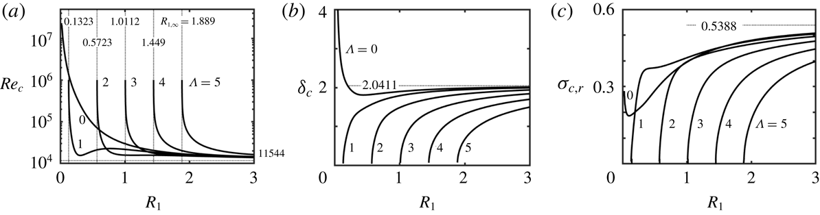
). Their results were reproduced as a part of the present study. Data displayed in figure 4(a) demonstrate that different waves play the critical role depending on the radius
 $R_{1}$
. The axisymmetric waves dominate for
 $R_{1}>3.372$
and
 $R_{1}<0.132$
. In the case of large enough
 $R_{1}$
, the critical Reynolds number is
 $Re_{c}\rightarrow 11\,544$
when
 $R_{1}\rightarrow \infty$
, which is the plane Poiseuille flow limit if one accounts for different scaling (Orszag Reference Orszag1971). Reduction of
 $R_{1}$
gives preference to different spiral waves: waves with
 $\unicode[STIX]{x1D6EC}=1$
dominate for
 $0.1323<R_{1}<0.7157$
and
 $3.184<R_{1}<3.372$
; waves with
 $\unicode[STIX]{x1D6EC}=2$
dominate for
 $0.7157<R_{1}<1.944$
and
 $2.362<R_{1}<3.184$
; and waves with
 $\unicode[STIX]{x1D6EC}=3$
dominate for
 $1.944<R_{1}<2.362$
; other oblique waves never play the dominant role. The spiral waves become unconditionally stable when
 $R_{1}<R_{1,\infty }$
, where
 $R_{1,\infty }$
plays the role of a limit point, whereas the axisymmetric waves are always conditionally stable as
 $Re_{c}\rightarrow \infty$
when
 $R_{1}\rightarrow 0$
. The results displayed in figure 4(b,c) exhibit similar trends, i.e. the critical axial wavenumber,
 $\unicode[STIX]{x1D6FF}_{c}$
, and the critical phase speed,
 $\unicode[STIX]{x1D70E}_{r,c}$
, approach the plane flow limit when
 $R_{1}\rightarrow \infty$
;
 $\unicode[STIX]{x1D6FF}_{c}$
and
 $\unicode[STIX]{x1D70E}_{r,c}$
of the spiral waves approach zero when
 $R_{1}\rightarrow R_{1,\infty }$
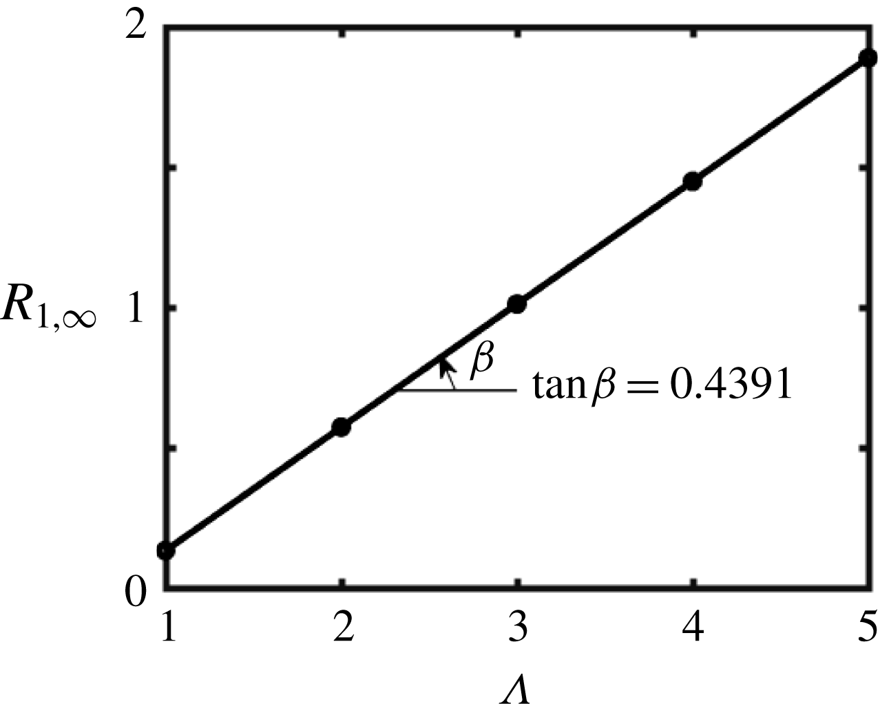
. The results displayed in figure 5 demonstrate that
 $R_{1,\infty }$
changes linearly with the circumferential wavenumber
 $\unicode[STIX]{x1D6EC}$
and its variations can be approximated as
 $R_{1,\infty }=0.4391\unicode[STIX]{x1D6EC}-0.3062$
.
Variations of (a) the critical Reynolds number
 $Re_{c}$
, (b) the critical axial wavenumber
 $\unicode[STIX]{x1D6FF}_{c}$
and (c) the critical frequency
 $\unicode[STIX]{x1D70E}_{c,r}=\text{Re}(\unicode[STIX]{x1D70E}_{c})$
in a smooth annulus as functions of the radius
 $R_{1}$
for different disturbance circumferential wavenumbers
 $\unicode[STIX]{x1D6EC}$
. The thin vertical dotted lines in (a) identify radii
 $R_{1,\infty }$
where
 $Re_{c}\rightarrow \infty$
. The thin horizontal dotted lines identify asymptotes for
 $R_{1}\rightarrow \infty$
.

Variations of
 $R_{1,\infty }$
as a function of the spiral wave circumferential wavenumber,
 $\unicode[STIX]{x1D6EC}$
.

4.2 Tollmien–Schlichting waves in grooved annuli
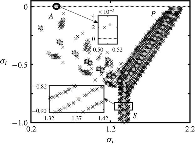
Figure 6 displays a typical
 $\unicode[STIX]{x1D70E}$
-spectrum for a grooved annulus for conditions where the flow in the smooth annulus with the same
 $R_{1}$
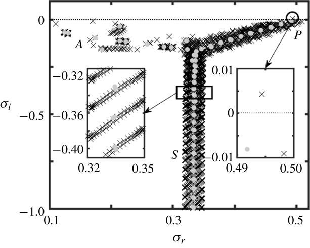
is unstable. The form of this spectrum is similar to the smooth-annulus spectrum and consists of the Airy (
 $A$
-branch), Pekeris (
 $P$
-branch), and Schensted (
 $S$
-branch) branches (Mack Reference Mack1976). The unstable mode is located at the top of the
 $A$
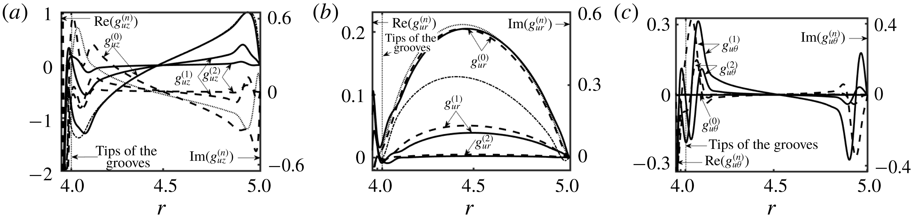
-branch and thus it represents the ‘wall mode’ (Mack Reference Mack1976; Schmid Reference Schmid2007). The results show that this mode is attenuated by the grooves;
 $g_{uz}^{(n)}$
is the dominant eigenfunction as illustrated in figure 7, with
 $g_{ur}^{(n)}$
and
 $g_{u\unicode[STIX]{x1D703}}^{(n)}$
being an order of magnitude smaller;
 $g_{uz}^{(n)}$
and
 $g_{u\unicode[STIX]{x1D703}}^{(n)}$
have maxima close to the walls, while
 $g_{ur}^{(n)}$
is dominant at the mid-section of the annulus. Comparisons with the eigenfunctions for the smooth annulus demonstrate that grooves only slightly alter these eigenfunctions and, at the same time, activate higher Fourier modes. This suggests that the unstable waves in the grooved annulus should have similar characteristics as waves in the smooth annulus.
The
 $\unicode[STIX]{x1D70E}$
-spectrum for an annulus with geometry described by (2.11) with
 $R_{1}=4$
,
 $S=0.025$
and
 $M=5$
for
 $Re=15\,000$
and axisymmetric disturbances (
 $\unicode[STIX]{x1D6EC}=0$
) with the axial wavenumber
 $\unicode[STIX]{x1D6FF}=2.04$
. Grey circles identify the spectrum for a smooth annulus for the same conditions.

Eigenfunctions for the unstable eigenvalue from figure 6 normalized with
 $\max _{R_{1}+0.5\leqslant r\leqslant 1+R_{1}}\text{Re}(g_{uz}^{(0)})=1$
. Panels (a–c) display
 $g_{uz}^{(n)}(r)$
,
 $g_{ur}^{(n)}(r)$
and
 $g_{u\unicode[STIX]{x1D703}}^{(n)}(r)$
, respectively, for
 $n=0$
, 1 and 2. Solid (dashed) lines represent the real (imaginary) parts. Thin dash-dotted (dotted) lines represent the real (imaginary) part of the eigenfunction for the unstable eigenvalue for the smooth annulus.

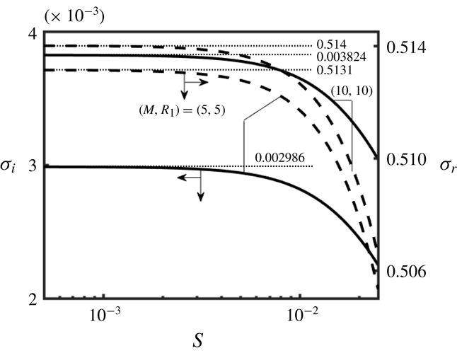
Results of tracing of complex frequencies as functions of the groove amplitude
 $S$
displayed in figure 8 demonstrate that the unstable modes connect to the unstable TS waves in the smooth annuli limit
 $(S\rightarrow 0)$
. The amplification rates decrease rapidly as the groove amplitude increases, suggesting a stabilizing effect for conditions used in figure 8.
Variations of the amplification rate
 $\unicode[STIX]{x1D70E}_{i}$
(solid lines) and the frequency
 $\unicode[STIX]{x1D70E}_{r}$
(dashed lines) for the axisymmetric disturbances with the axial wavenumber
 $\unicode[STIX]{x1D6FF}=2.04$
as functions of the groove amplitude
 $S$
for the TS instability in an annulus described by (2.11) for
 $Re=15\,000$
. Thin dotted lines identify the smooth annuli limits
 $(S\rightarrow 0)$
.

Critical stability conditions can be determined by tracing the most unstable eigenvalue through the
 $(Re{-}\unicode[STIX]{x1D6FF})$
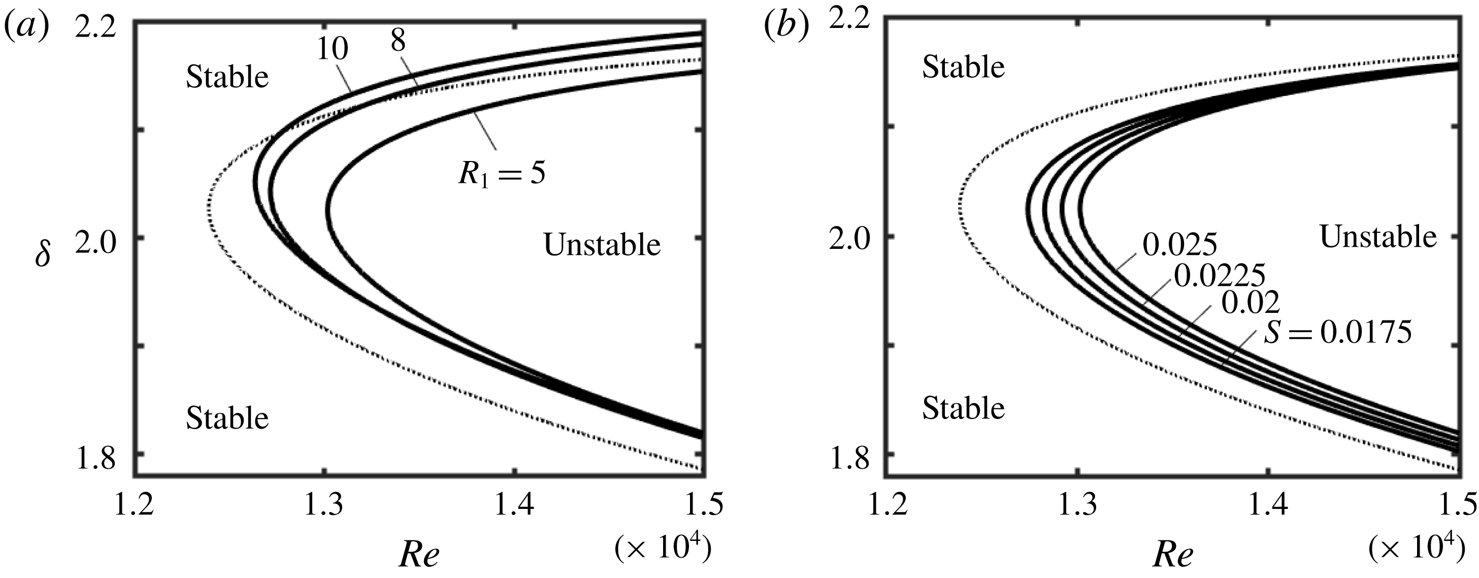
-plane. Figure 9 displays the resulting neutral stability curves for various geometries. The critical Reynolds number,
 $Re_{c}$
, corresponds to the leftmost tip of each curve and the associated
 $\unicode[STIX]{x1D6FF}$
is referred to as the critical axial wavenumber
 $\unicode[STIX]{x1D6FF}_{c}$
. In general, a decrease of the radius
 $R_{1}$
and an increase of the groove amplitude
 $S$
result in an increase of
 $Re_{c}$
, with the smooth annulus with the largest
 $R_{1}$
representing the most unstable geometry. The critical axial wavenumber
 $\unicode[STIX]{x1D6FF}_{c}$
changes negligibly with
 $S$
and varies within 5 % as a function of
 $R_{1}$
.
Neutral stability curves in the
 $(Re{-}\unicode[STIX]{x1D6FF})$
-plane for the axisymmetric disturbances
 $(\unicode[STIX]{x1D6EC}=0)$
for the TS instability in an annulus described by (2.11) with
 $M=5$
. (a) Results for
 $S=0.025$
and different
 $R_{1}$
, and (b) results for
 $R_{1}=5$
and different
 $S$
. Thin dotted lines identify the neutral stability curves for a smooth annulus with
 $R_{1}=5$
.

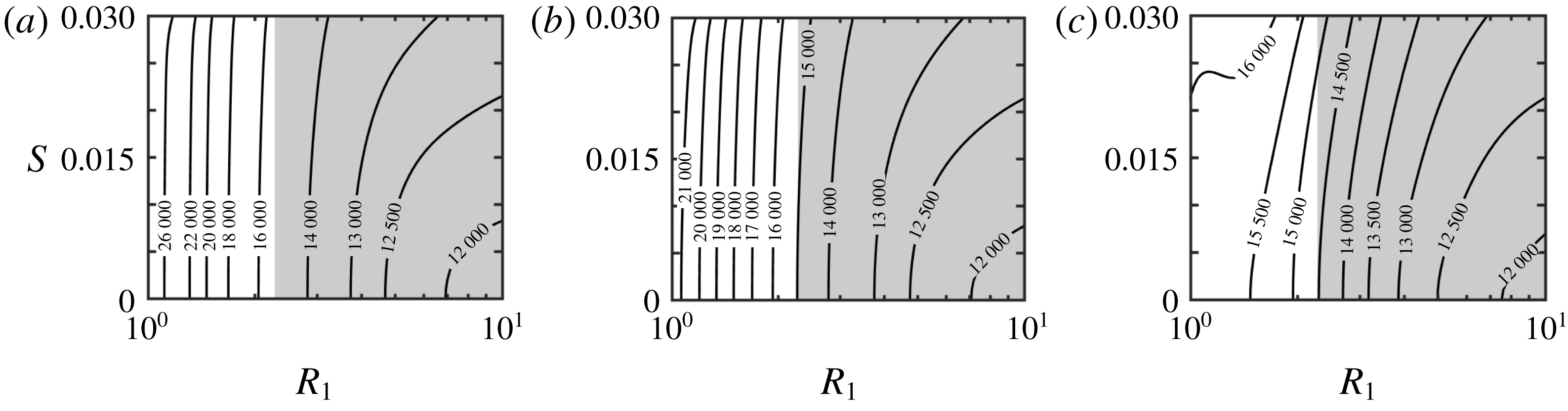
Figure 10 provides a compact summary of variations of
 $Re_{c}$
as a function of geometric parameters (
 $R_{1}$
and
 $S$
) for the axisymmetric and spiral waves. Grooves stabilize all waves, as
 $Re_{c}$
is always larger than that in the smooth annulus with the same
 $R_{1}$
. The minimum of
 $Re_{c}$
corresponds to the maximum
 $R_{1}$
considered in this study
 $(R_{1}=10)$
. Figure 10(a,b) demonstrates that
 $Re_{c}$
increases monotonically with an increase of
 $R_{1}$
for the axisymmetric and spiral waves with
 $\unicode[STIX]{x1D6EC}=1$
, which is analogous to the smooth annuli for
 $1\leqslant R_{1}\leqslant 10$
(see figure 10
a). Figure 10(c) demonstrates that the dominant role of the spiral waves with
 $\unicode[STIX]{x1D6EC}=2$
is preserved for
 $R_{1}\lesssim 2$
.
Variations of the critical Reynolds number
 $Re_{c}$
as a function of
 $R_{1}$
and
 $S$
for the TS waves in an annulus described by (2.11) with
 $M=5$
. (a–c) Results for waves with the circumferential wavenumbers
 $\unicode[STIX]{x1D6EC}=0$
, 1 and 2, respectively. The
 $Re_{c}$
value for the grooved annulus is larger than
 $Re_{c}$
for the smooth annulus for the geometric conditions used in this figure. Shaded areas correspond to the drag-reducing configurations.

It should not be surprising that grooves stabilize TS waves. These waves are driven by friction, with the active zones of energy transfer from the primary to the secondary flows located in the vicinity of critical layers and near the solid walls. Reduction of shear drag suggests reduced effectiveness of shear near the walls, which should weaken the energy transfer. Groove-induced flow modifications affect conditions near the critical layers but the type of change of energy transfer cannot be predicted. Detailed computations demonstrate an increase of the critical Reynolds number even for the drag-increasing configurations, which suggests that the energy transfer mechanism near the critical layer is weakened by the grooves.
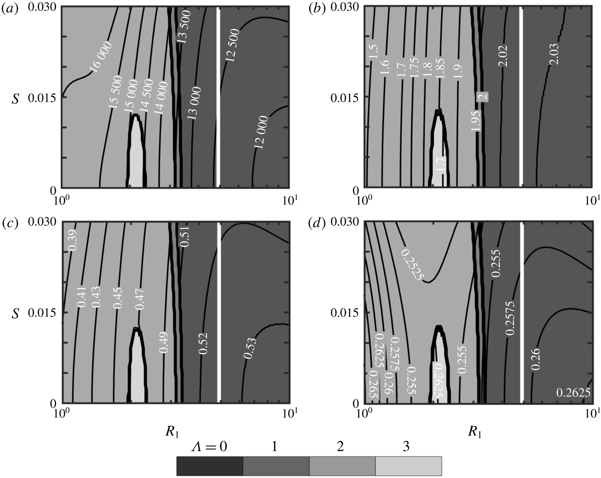
Figure 11(a) illustrates variations of the minimum of
 $Re_{c}$
in annuli with
 $M=10$
for all relevant waves, i.e.
 $\unicode[STIX]{x1D6EC}=0$
, 1, 2 and 3, and identifies zones where each wave dominates. The axisymmetric waves are dominant for
 $R_{1}\gtrsim 2.5$
while the spiral waves dominate at smaller
 $R_{1}$
values. Since this trend is similar to the smooth annuli case, one can conclude that grooves do not change the form of the dominant TS wave. Figure 11(b,c) illustrates variations of the critical axial wavenumber,
 $\unicode[STIX]{x1D6FF}_{c}$
, and the critical frequency,
 $\unicode[STIX]{x1D70E}_{r,c}=\text{Re}(\unicode[STIX]{x1D70E}_{c})$
. The values of
 $\unicode[STIX]{x1D6FF}_{c}$
and
 $\unicode[STIX]{x1D70E}_{r,c}$
decrease with decreasing
 $R_{1}$
and are almost independent of the groove amplitude. The critical phase speed
 $c_{c}=\unicode[STIX]{x1D70E}_{r,c}\unicode[STIX]{x1D6FF}_{c}$
changes in a narrow range between 0.25 and 0.268, as illustrated in figure 11(d), in spite of the wide range of variations of
 $\unicode[STIX]{x1D6FF}_{c}$
and
 $\unicode[STIX]{x1D70E}_{r,c}$
. Similar computations carried out for other values of
 $M$
resulted in similar trends and thus are not presented.
Variations of (a) the critical Reynolds number
 $Re_{c}$
, (b) the critical wavenumber
 $\unicode[STIX]{x1D6FF}_{c}$
, (c) the critical frequency
 $\unicode[STIX]{x1D70E}_{r,c}$
and (d) the critical phase speed
 $c_{c}=\unicode[STIX]{x1D70E}_{r,c}/\unicode[STIX]{x1D6FF}_{c}$
as functions of
 $R_{1}$
and
 $S$
for the TS instability in an annulus described by (2.11) with
 $M=10$
. The background colours identify zones of dominance of different waves (
 $\unicode[STIX]{x1D6EC}=0$
, axisymmetric waves;
 $\unicode[STIX]{x1D6EC}\neq 0$
, spiral waves). The discontinuities of
 $\unicode[STIX]{x1D6FF}_{c}$
,
 $\unicode[STIX]{x1D70E}_{r,c}$
and
 $c_{c}$
in (b–d) are associated with changes of
 $\unicode[STIX]{x1D6EC}$
. Zones to the right of the thick white solid lines correspond to the drag-reducing configurations. The
 $Re_{c}$
value for the grooved annulus is smaller than
 $Re_{c}$
for the smooth annulus for conditions used in the above figures.

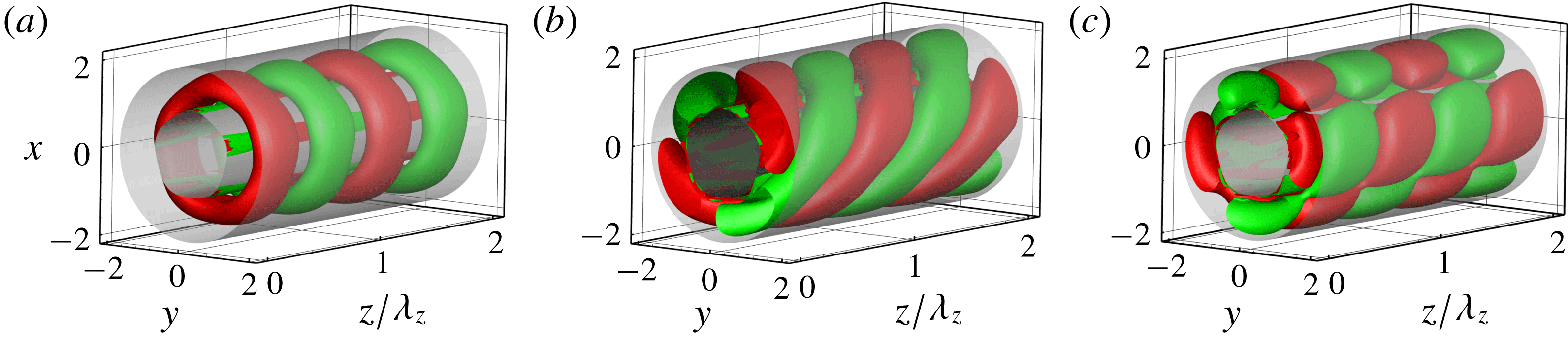
The above discussion shows that a variety of possible secondary states may be formed at the onset depending on the radius
 $R_{1}$
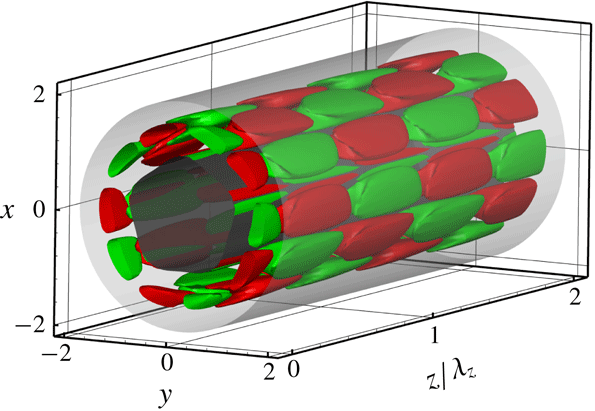
. Figure 12(a) illustrates the topology of an axisymmetric wave which has the form of axisymmetric rings. Figure 12(b) illustrates the topology associated with a single spiral wave which has the form of helical rings with a specific pitch angle
 $\unicode[STIX]{x1D6FD}=\tan ^{-1}(R_{1}\unicode[STIX]{x1D6FF}_{c}/\unicode[STIX]{x1D6EC})\approx 36^{\circ }$
. Figure 12(c) illustrates one of the possible topologies resulting from a superposition of two spiral waves with the opposite twists. As both waves have the same onset conditions, the resulting topology is dictated by their relative strength. There is a continuous spectrum of such topologies, with the one displayed in figure 12(c) corresponding to waves of equal amplitudes producing rhombic structures. These structures are very similar to helical stripe patterns found in a direct numerical simulation of transitional APF (Ishida et al.
Reference Ishida, Duguet and Tsukahara2016). All structures are not directly related to the groove geometries but are dictated by the critical disturbance wavenumbers.
The disturbance velocity field in an annulus described by (2.11) with
 $R_{1}=1$
,
 $M=5$
and
 $S=0.03$
at the onset of the TS instability normalized with
 $\max _{R_{1}+0.5\leqslant r\leqslant 1+R_{1}}\text{Re}(g_{uz}^{(0)})=1$
. (a–c) Isosurfaces of
 $u_{rD}$
at the instability onset (a) for the axisymmetric waves (
 $\unicode[STIX]{x1D6EC}=0$
,
 $Re_{c}=35\,806$
,
 $\unicode[STIX]{x1D6FF}_{c}=1.779$
), (b) for a single spiral wave (
 $\unicode[STIX]{x1D6EC}=2$
,
 $Re_{c}=16\,389$
,
 $\unicode[STIX]{x1D6FF}_{c}=1.451$
) and (c) for a system of two opposite spiral waves of equal amplitudes (
 $\unicode[STIX]{x1D6EC}=\pm 2$
,
 $Re_{c}=16\,389$
,
 $\unicode[STIX]{x1D6FF}_{c}=1.451$
). Red (green) colours used mark isosurfaces corresponding to
 $u_{rD}=0.15$
(
 $u_{rD}=-0.15$
).

4.3 A new class of waves in grooved annuli
It was suggested at the beginning of this paper that circumferential variations of the axial velocity component may activate an instability mechanism, giving rise to a different secondary flow. An extensive search through the parameter space resulted in the identification of a different class of unstable travelling waves. Figure 13 displays a typical
 $\unicode[STIX]{x1D70E}$
-spectrum for this situation. This spectrum consists of the
 $A$
-,
 $P$
- and
 $S$
-branches and thus has a structure similar to the TS spectrum. All elements of the
 $A$
-branch are attenuated for both smooth and grooved annuli. Grooves destabilize the top element of the
 $P$
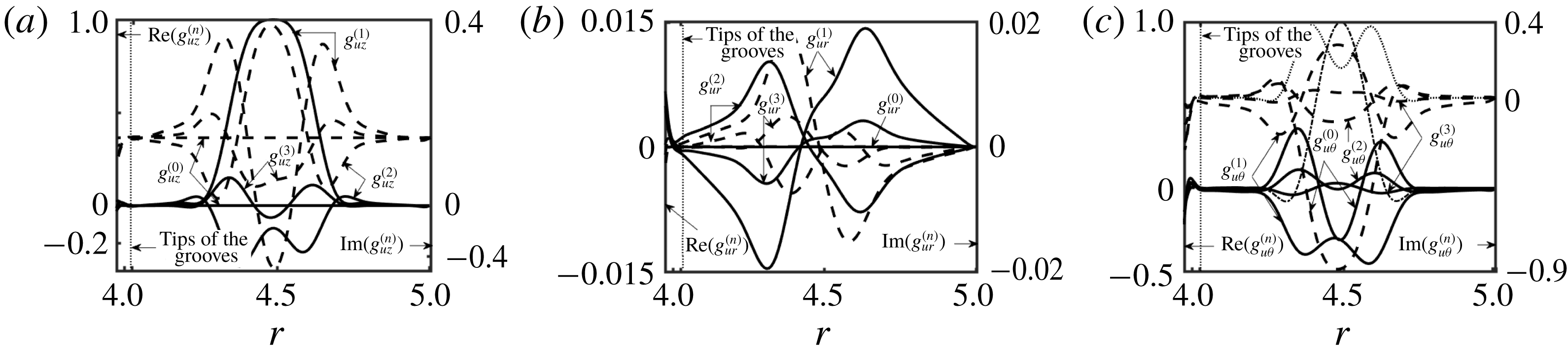
-branch, which represents the ‘centre mode’ (Mack Reference Mack1976; Schmid & Henningson Reference Schmid and Henningson2001; Drazin & Reid Reference Drazin and Reid2004); this element is attenuated in the smooth annuli. The corresponding eigenfunctions have peaks at the mid-section of the annulus (away from the walls), which is a characteristic feature of modes forming the
 $P$
-branch (see figure 14). The values of
 $g_{uz}^{(n)}(r)$
and
 $g_{u\unicode[STIX]{x1D703}}^{(n)}(r)$
are of similar magnitudes while
 $g_{ur}^{(n)}(r)$
is two orders of magnitude smaller. The new mode creates an almost planar motion in the
 $(\unicode[STIX]{x1D703}{-}z)$
-plane, concentrated in the mid-section of the annulus. The dominant Fourier mode corresponds to index
 $n=1$
rather than 0, as was the case for the TS waves. Thus, the characteristics of the disturbance velocity field created by this instability are very different from the TS velocity field. The dominance of mode
 $n=1$
indicates that grooves are essential for the formation of these waves.
The
 $\unicode[STIX]{x1D70E}$
-spectrum for the new instability for an annulus described by (2.11) with
 $R_{1}=4$
,
 $S=0.025$
and
 $M=5$
for
 $Re=15\,000$
and the axisymmetric disturbances
 $(\unicode[STIX]{x1D6EC}=0)$
with the axial wavenumber
 $\unicode[STIX]{x1D6FF}=0.6$
. Grey circles identify the spectrum for a smooth annulus for the same conditions.

Eigenfunctions for the unstable eigenvalue from figure 13 normalized with
 $\max _{R_{1}+0.5\leqslant r\leqslant 1+R_{1}}\text{Re}(g_{uz}^{(1)})=1$
. Panels (a–c) display
 $g_{uz}^{(n)}(r)$
,
 $g_{ur}^{(n)}(r)$
and
 $g_{u\unicode[STIX]{x1D703}}^{(n)}(r)$
, respectively, for
 $n=0$
, 1, 2 and 3. Solid (dashed) lines represent the real (imaginary) parts. Thin dash-dotted (dotted) lines represent the real (imaginary) part of the eigenfunction for the least stable eigenvalue for the smooth annulus.

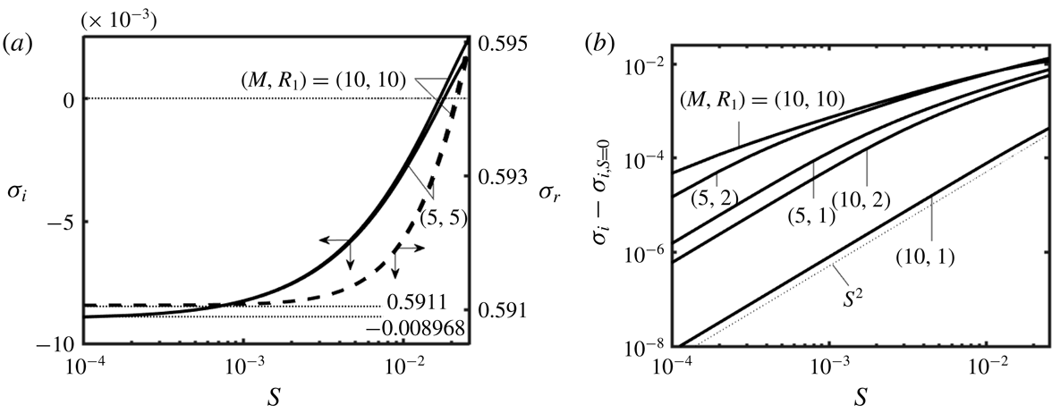
The results of tracing of complex frequencies as functions of the groove amplitude
 $S$
displayed in figure 15 demonstrate that the unstable mode connects to the least stable element of the
 $P$
-branch in the spectrum for the smooth annulus. The waves are highly attenuated in the limit of
 $S\rightarrow 0$
but their amplification rates increase proportionally to
 $S^{2}$
(see figure 15
b) and they begin to grow when the amplitude reaches the level of
 $S\approx 0.01$
. The frequencies of these waves change marginally with
 $S$
and they are not too different from the frequencies of the TS waves (compare figure 8 and figure 15
a).
Variations of the amplification rate
 $\unicode[STIX]{x1D70E}_{i}$
(solid lines) and the frequency
 $\unicode[STIX]{x1D70E}_{r}$
(dashed lines) for the new instability for the axisymmetric
 $(\unicode[STIX]{x1D6EC}=0)$
waves with the axial wavenumber
 $\unicode[STIX]{x1D6FF}=0.6$
as a function of the groove amplitude
 $S$
for geometry described by (2.11) for
 $Re=15\,000$
. Panel (a) displays
 $\unicode[STIX]{x1D70E}_{i}$
and
 $\unicode[STIX]{x1D70E}_{r}$
, with the thin dotted lines identifying limits for
 $S\rightarrow 0$
. Panel (b) displays the difference
 $(\unicode[STIX]{x1D70E}_{i}-\unicode[STIX]{x1D70E}_{i,S=0})$
, where
 $\unicode[STIX]{x1D70E}_{i,S=0}$
stands for the amplification rate in a smooth annulus and the thin dotted line identifies the characteristic slope.

It was shown earlier (see § 4.2) that the radius
 $R_{1}$
dictates the type of the dominant TS wave, i.e. the axisymmetric waves are dominant for large
 $R_{1}$
values and spiral waves are dominant for small
 $R_{1}$
values. The results presented in figure 16 suggest that the axisymmetric new waves have amplification higher than the spiral waves. This suggests that Squire’s theorem (Squire Reference Squire1933) is valid and thus it is sufficient to focus analysis on the axisymmetric waves only. Figure 17 demonstrates that the flow topology has the form of rectangular patches propagating with a certain speed in the axial direction with their circumferential size dictated by the groove wavelength and the axial size dictated by the critical disturbance wavenumber and thus it is very different from the TS wave topology (see figure 12
a).
Variations of the amplification rate
 $\unicode[STIX]{x1D70E}_{i}$
for the new instability as a function of the axial wavenumber
 $\unicode[STIX]{x1D6FF}$
for the geometry described by (2.11) with
 $M=5$
for
 $Re=15\,000$
and different circumferential wavenumbers
 $\unicode[STIX]{x1D6EC}$
. The solid, dashed and dash-dotted lines correspond to annuli with
 $R_{1}=2$
, 5 and 10, respectively.

The disturbance field in an annulus with the geometry described by (2.11) with
 $R_{1}=1$
,
 $M=5$
and
 $S=0.05$
at the onset of the new axisymmetric wave, i.e.
 $Re_{c}=3626$
and
 $\unicode[STIX]{x1D6FF}_{c}=1.50$
. Eigenfunctions are normalized with
 $\max _{R_{1}+0.5\leqslant r\leqslant 1+R_{1}}\text{Re}(g_{uz}^{(1)})=1$
. The positive and negative isosurfaces
 $u_{zD}=\pm 0.9$
are marked using red and green colours, respectively.

The critical stability conditions can be determined by tracing the most unstable eigenvalue through the
 $(Re{-}\unicode[STIX]{x1D6FF})$
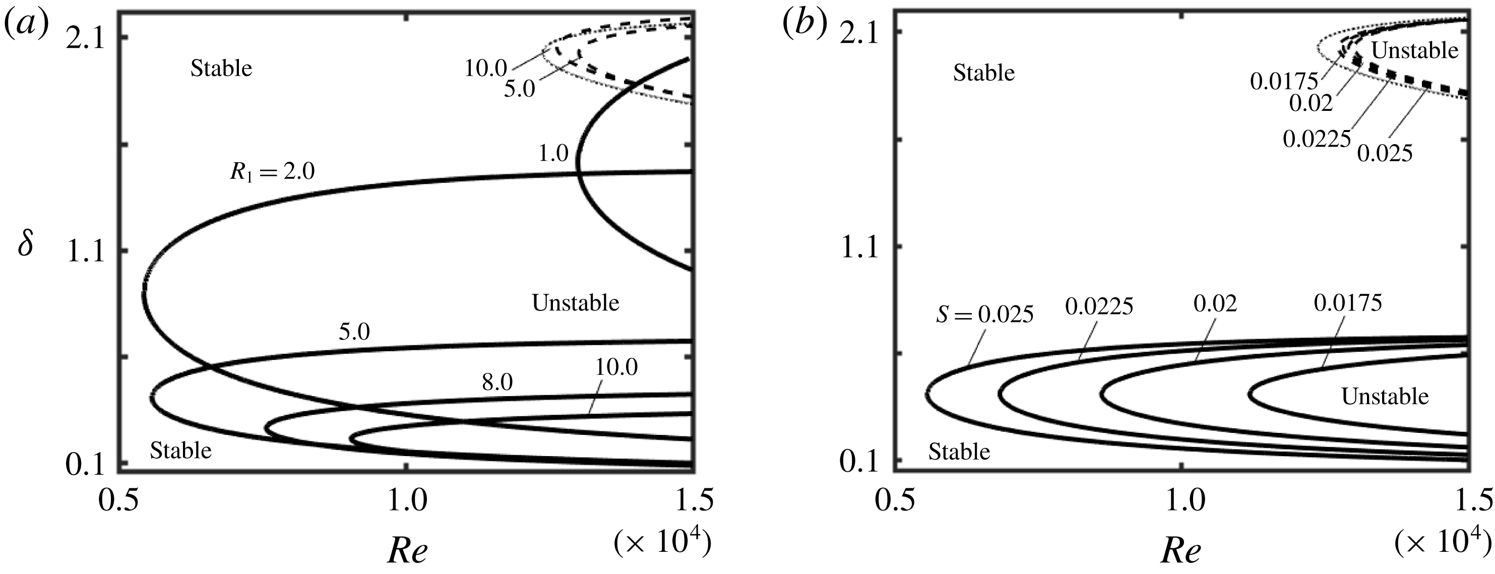
-plane. Figure 18 displays the resulting neutral stability curves. Curves for the new mode are shifted towards smaller
 $\unicode[STIX]{x1D6FF}$
than those for the TS waves, and the critical Reynolds numbers are smaller by an order of magnitude than those for the TS waves (see figure 18
a). Radius
 $R_{1}$
has a strong impact on
 $Re_{c}$
, with
 $Re_{c}$
first decreasing rapidly with an increase of
 $R_{1}$
, reaching a minimum and then increasing. The position of the minimum depends on the number of grooves
 $M$
; it occurs at
 $R_{1}\approx 3$
for the conditions used in figure 18(a), at
 $R_{1}\approx 0.95$
for
 $M=2$
and at
 $R_{1}\approx 6.4$
for
 $M=10$
. It is marginally affected by
 $S$
as illustrated in figure 18(b). The critical axial wavenumber
 $\unicode[STIX]{x1D6FF}_{c}$
changes drastically with
 $R_{1}$
, always decreasing with increasing
 $R_{1}$
(see figure 18
a). An increase of the groove amplitude rapidly decreases
 $Re_{c}$
while marginally affecting
 $\unicode[STIX]{x1D6FF}_{c}$
(see figure 18
b).
The neutral stability curves in the
 $(Re{-}\unicode[STIX]{x1D6FF})$
-plane for the axisymmetric
 $(\unicode[STIX]{x1D6EC}=0)$
waves in an annulus with geometry described by (2.11) with
 $M=5$
. (a) Results for
 $S=0.025$
and representative
 $R_{1}$
. (b) Results for
 $R_{1}=5$
and representative
 $S$
. Solid and dashed lines correspond to the new waves and the TS waves, respectively. Thin dotted lines identify the neutral stability curves for the TS waves in a smooth annulus with
 $R_{1}=5$
.

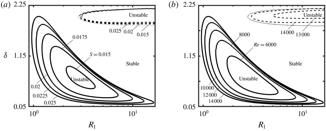
The effects of variations of radius
 $R_{1}$
on the onset conditions are illustrated in figure 19, which displays the neutral stability curves in the
 $(R_{1}{-}\unicode[STIX]{x1D6FF})$
-plane. The unstable region is confined to a finite range of
 $R_{1}$
bounded from above and from below, i.e. the new waves do not exist in annuli with a fixed number of grooves with
 $R_{1}$
values that are either too small or too large. The unstable zone expands by increasing both
 $S$
and
 $Re$
. Radius
 $R_{1}\approx 3$
is the most destabilizing for
 $M$
used in figure 19 in the sense that it requires the smallest groove amplitude and the smallest Reynolds number to create a secondary flow. It should be stressed that the new waves and the TS waves appear at different ranges of
 $R_{1}$
and
 $\unicode[STIX]{x1D6FF}$
.
The neutral stability curves in the
 $(R_{1}{-}\unicode[STIX]{x1D6FF})$
-plane for the axisymmetric new waves in an annulus with geometry described by (2.11) with
 $M=5$
. (a) Results for
 $Re=14\,000$
and different
 $S$
; and (b) results for
 $S=0.025$
and different
 $Re$
. Dashed lines show similar results for the TS waves. Thin dotted lines identify the neutral stability curves for the TS waves in smooth annuli for
 $Re=14\,000$
.

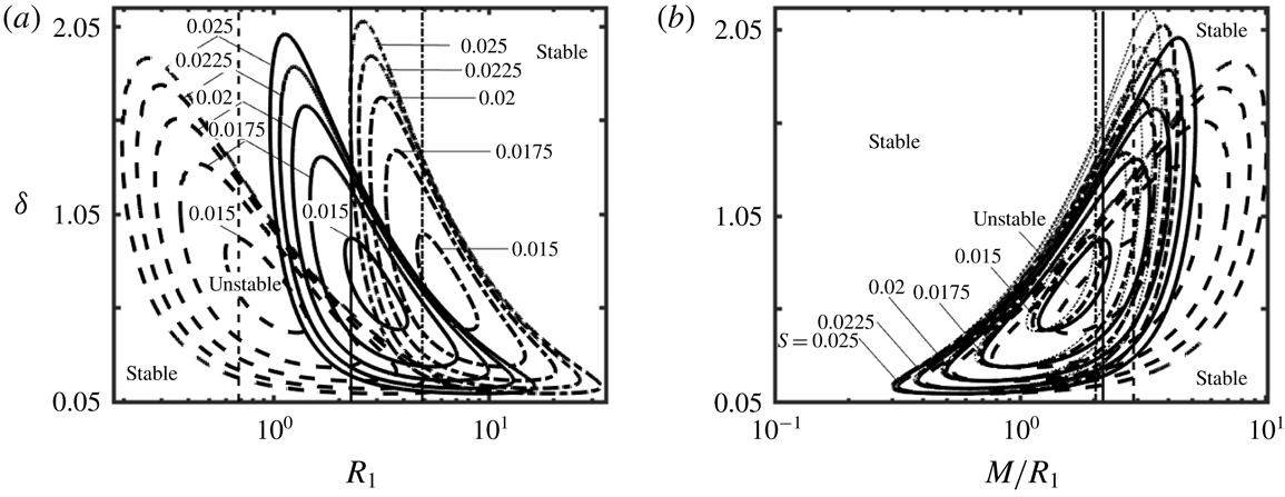
The same procedure repeated for
 $M=2$
and 10 demonstrates that the neutral stability curves have the same form but shift towards higher
 $R_{1}$
and slightly expand in the
 $\unicode[STIX]{x1D6FF}$
-direction as
 $M$
increases (see figure 20
a). This shift results from changes of the groove wavelength
 $\unicode[STIX]{x1D706}_{\unicode[STIX]{x1D703}}=2\unicode[STIX]{x03C0}R_{1}/M$
, which depends on both the number of grooves
 $M$
and the radius
 $R_{1}$
(or the cylinder circumference). The same results re-plotted in figure 20(b) using
 $M/R_{1}$
rather than
 $R_{1}$
show a much better overlap of the neutral curves for different geometries as well as their evolution towards the plane channel limit
 $(R_{1}\rightarrow \infty )$
.
(a) The neutral stability curves in the
 $(R_{1}{-}\unicode[STIX]{x1D6FF})$
-plane for the new axisymmetric waves in an annulus with geometry described by (2.11) for
 $Re=14\,000$
. Dashed, solid and dash-dotted lines correspond to annuli with
 $M=2$
, 5 and 10, respectively. (b) The same results presented in terms of the groove wavenumber, i.e.
 $M/R_{1}$
, with dotted lines corresponding to the plane channel limit
 $(R_{1}\rightarrow \infty )$
. The thin vertical lines identify
 $R_{1,cutoff}$
for each
 $M$
. Zones to the right of
 $R_{1,cutoff}$
correspond to the drag-reducing configurations.

Figure 21 provides a compact summary of variations of the critical stability conditions for the new wave in an annulus with
 $M=2$
as functions of
 $R_{1}$
and
 $S$
. The variations of
 $Re_{c}$
illustrated in figure 21(a) demonstrate that an increase of the groove amplitude decreases
 $Re_{c}$
for all
 $R_{1}$
values. There exists an
 $R_{1}$
that results in the smallest
 $Re_{c}$
for a given
 $S$
, which we shall refer to as
 $R_{1,min}$
;
 $R_{1,min}$
changes marginally with
 $S$
. It is interesting to note that
 $Re_{c}$
changes proportionally to
 $S^{-2}$
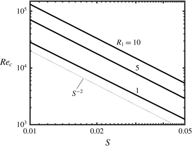
(see figure 22) which means that quite low
 $Re_{c}$
values can be achieved with large groove amplitudes. The lowest critical Reynolds number for
 $S\leqslant 0.05$
, which is the largest
 $S$
used in the present study, is
 $Re_{c}=1232$
, and it corresponds to the annulus with
 $R_{1}=1.0$
and
 $S=0.05$
. The results displayed in figure 21(b) demonstrate rapid changes of
 $\unicode[STIX]{x1D6FF}_{c}$
as a function of
 $R_{1}$
, with longer waves dominating for larger
 $R_{1}$
, but negligible variations as a function of
 $S$
. The results displayed in figure 21(c) demonstrate a similar pattern of variations of
 $\unicode[STIX]{x1D70E}_{r,c}$
, which decreases with an increase of
 $R_{1}$
and changes marginally with
 $S$
. Figure 21(c) also shows that
 $c_{c}=\unicode[STIX]{x1D70E}_{r,c}/\unicode[STIX]{x1D6FF}_{c}\approx 1$
for the whole range of variations of
 $S$
and
 $R_{1}$
; it is approximately four times larger than
 $c_{c}$
for the TS waves.
Variations of (a) the critical Reynolds number
 $Re_{c}$
, (b) the critical axial wavenumber
 $\unicode[STIX]{x1D6FF}_{c}$
and (c the critical frequency
 $\unicode[STIX]{x1D70E}_{r,c}$
(solid lines) and the critical phase speed
 $c_{c}=\unicode[STIX]{x1D70E}_{r,c}/\unicode[STIX]{x1D6FF}_{c}$
(dashed lines) for the onset of the new axisymmetric waves as functions of the radius
 $R_{1}$
and the groove amplitude
 $S$
for the geometry described by (2.11) with
 $M=2$
. Thin dotted lines identify
 $R_{1,min}$
(see text for definition) while the shaded areas correspond to the drag-reducing configurations.

Variations of the critical Reynolds number as a function of the groove amplitude for the geometry described by (2.11) with
 $M=2$
and suitable
 $R_{1}$
values.

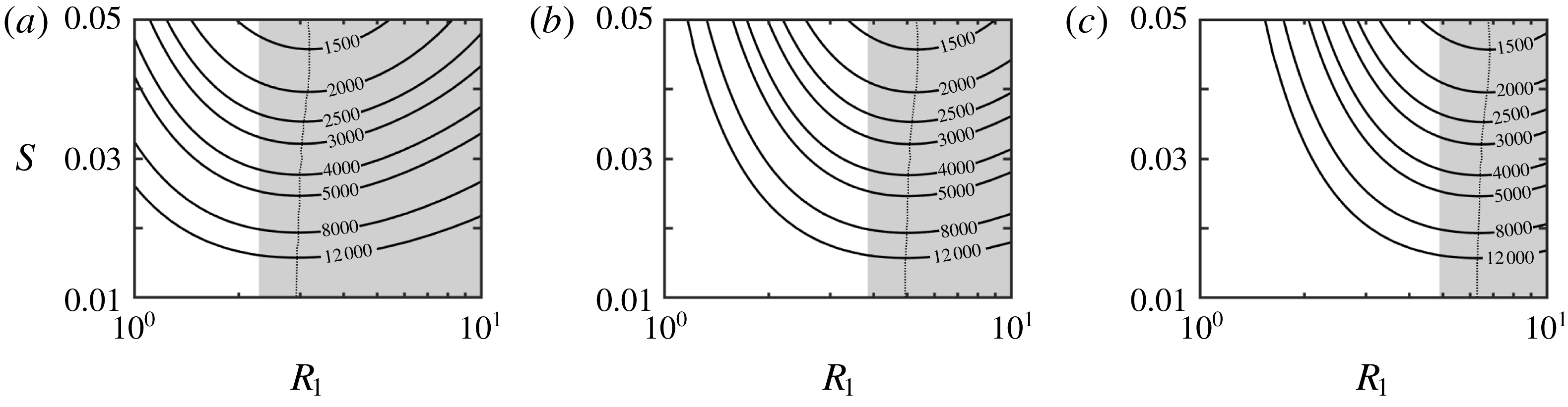
The same procedure was repeated for different numbers of grooves, i.e.
 $M=5$
, 8 and 10, with the relevant results displayed in figure 23. An increase of
 $M$
shifts
 $Re_{c}$
towards higher
 $R_{1}$
but does not affect its minimum. Also,
 $R_{1,min}$
shifts towards higher
 $R_{1}$
. The critical phase speed is almost constant for all configurations, i.e.
 $c_{c}\approx 1$
, and varies in a manner very similar to that displayed in figure 21(c) (details are not shown).
Variations of the critical Reynolds number
 $Re_{c}$
for the new waves as a function of
 $R_{1}$
and
 $S$
for geometries described by (2.11) for grooves with
 $M=5$
(a),
 $M=8$
(b) and
 $M=10$
(c). Thin dotted lines identify
 $R_{1,min}$
(see text for definition) while the shaded area identifies the drag-reducing configurations.

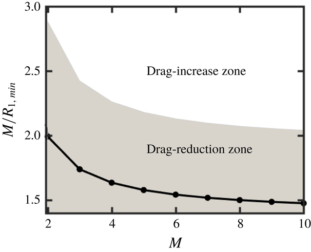
Data from figure 23 provide the basis for identification of geometries which promote the new wave at the smallest Reynolds number. The curve fitting shows that variations of
 $R_{1,min}$
as a function of
 $M$
can be approximated as
 $R_{1,min}=0.7213M-0.4391$
, which means that
 $M/R_{1,min}$
changes as
 $M/R_{1,min}=M/(0.7213M-0.4391)$
and has a limit of
 $M/R_{1,min}\rightarrow 1.4$
as
 $M\rightarrow \infty$
, i.e. its characteristics in this limit approach those of a plane channel (see figure 24). A comparison of
 $M/R_{1,min}$
and
 $(M/R_{1})_{cutoff}$
demonstrates that annular configurations which give the minimum
 $Re_{c}$
also reduce the frictional drag.
Variations of the effective groove wavenumber
 $M/R_{1,min}$
for the geometry described by (2.11) with
 $S=0.05$
as a function of
 $M$
. The shaded area identifies drag-reduction configurations, i.e.
 $M/R_{1}<(M/R_{1})_{cutoff}$
(see § 2 for details). The solid line represents the correlation discussed in the text.

4.4 Instability mechanisms
It is well known that TS waves are driven by friction, which is responsible for energy transfer from the primary to the secondary states, with this transfer concentrated near the critical layers and solid walls (Baines, Majumdar & Mitsudera Reference Baines, Majumdar and Mitsudera1996). The results discussed in § 2 demonstrate that the addition of grooves results in a reduction of the wall shear over a large range of configurations, which weakens the instability mechanism and leads to an increase of the critical Reynolds number. A smaller increase of
 $Re_{c}$
for the drag-increasing configurations suggests that change in the flow conditions around the critical layers overcomes the friction increase occurring at the walls.
The new secondary state discussed in § 4.3 must be associated with a different mechanism. The results displayed in figure 25(a) demonstrate that the amplification rate for the TS waves initially increases with an increase of the Reynolds number, reaches a maximum and then starts decreasing, with the critical wavenumber following the same pattern. This character of variations demonstrates the viscous nature of the driving mechanism. The amplification rate for the new waves increases monotonically with
 $Re$
(see figure 25
b) while the critical wavenumber changes marginally, which suggests the inviscid character of the driving mechanism.
Variations of the growth rate
 $\unicode[STIX]{x1D70E}_{i}$
of the axisymmetric TS waves (a) and the axisymmetric new waves (b) as functions of the axial wavenumber
 $\unicode[STIX]{x1D6FF}$
for the geometry described by (2.11) with
 $R_{1}=5$
,
 $M=5$
and
 $S=0.025$
.

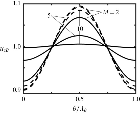
Circumferential variations of the axial velocity of the primary flow at the centre of the gap displayed in figure 26 demonstrate the formation of inflection points. The maximum of
 $u_{zB}$
occurs at the widest opening
 $(\unicode[STIX]{x1D703}/\unicode[STIX]{x1D706}_{\unicode[STIX]{x1D703}}=0.5)$
and the minimum at the smallest opening
 $(\unicode[STIX]{x1D703}/\unicode[STIX]{x1D706}_{\unicode[STIX]{x1D703}}=0)$
. The inflection points with
 $\unicode[STIX]{x2202}^{2}u_{zB}/\unicode[STIX]{x2202}\unicode[STIX]{x1D703}^{2}=0$
are located at
 $\unicode[STIX]{x1D703}/\unicode[STIX]{x1D706}_{\unicode[STIX]{x1D703}}\approx 0.25$
and 0.75. It is known that the existence of an inflection point in the transverse velocity distribution is the necessary condition for the inviscid instability (Rayleigh Reference Rayleigh1880; Fjørtoft Reference Fjørtoft1950), while an equivalent conclusion was reached for velocity profiles with spanwise variations (Henningson Reference Henningson1987). The driving mechanism is associated with vorticity dynamics while the instability is opposed by friction. The effectiveness of friction can be measured using the Reynolds number. The local conditions along the circumference are better captured using the local velocity maximum, which leads to the local Reynolds number defined as
 $Re_{loc}=Reu_{zB,max}$
;
 $Re_{loc}$
is largest in the widest opening and the secondary flow is thus expected to concentrate between the inflection points and the widest annulus opening.
Variations of
 $u_{zB}$
at
 $r=R_{1}+0.5$
for annuli described by (2.11) with
 $S=0.05$
,
 $R_{1}=1$
(solid lines) and
 $R_{1}=10$
(dashed lines).

To better illustrate the competition between the driving and opposing forces, consider the distribution of the radial component of vorticity of the primary flow
 $\unicode[STIX]{x1D702}_{B}=r^{-1}\unicode[STIX]{x2202}u_{zB}/\unicode[STIX]{x2202}\unicode[STIX]{x1D703}$
(Thorpe Reference Thorpe1969) as well as the distribution of the dissipation function of the primary flow (Lin Reference Lin1945; Bayly, Orszag & Herbert Reference Bayly, Orszag and Herbert1988) defined as
 $$\begin{eqnarray}\unicode[STIX]{x1D6F7}_{B}=\frac{1}{Re}\left[\left(\frac{1}{r}\frac{\unicode[STIX]{x2202}u_{zB}}{\unicode[STIX]{x2202}\unicode[STIX]{x1D703}}\right)^{2}+\left(\frac{\unicode[STIX]{x2202}u_{zB}}{\unicode[STIX]{x2202}r}\right)^{2}\right].\end{eqnarray}$$
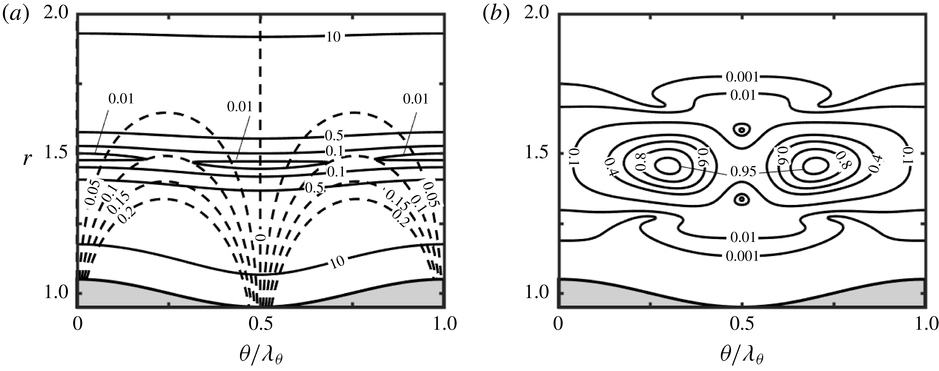
The dissipation function has a minimum at the mid-section of the annulus and increases towards the walls (see figure 27
a). The magnitude of vorticity is largest near the corrugated wall and decreases with distance away from it, with the local maxima in the circumferential directions located at
 $\unicode[STIX]{x1D703}/\unicode[STIX]{x1D706}_{\unicode[STIX]{x1D703}}\approx 0.25$
and 0.75 (see figure 27
a). The disturbance motion is expected to be the most intense in the zone where the ratio of vorticity (the driving force) and the dissipation (the opposing force) is the most beneficial, which is in the gap mid-section and around the inflection points. The distribution of the disturbance kinetic energy displayed in figure 27(b) confirms this prediction and demonstrates a small preference for the widest annulus opening.
(a) Distributions of the dissipation function
 $\unicode[STIX]{x1D6F7}_{B}$
(solid lines) and modulus of the radial vorticity component
 $|\unicode[STIX]{x1D702}_{B}|$
(dashed lines) of the primary flow in the annulus described by (2.11) with
 $R_{1}=1$
,
 $S=0.05$
and
 $M=5$
. (b) The distribution of the disturbance kinetic energy for the same conditions.

It has been shown in § 4.3 that
 $Re_{c}$
has minima at
 $R_{1,min}$
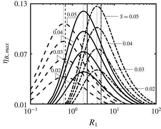
. The positions of these minima well correlate with the distributions of the primary flow vorticity. Figure 28 displays the variations of the maximum of vorticity
 $\unicode[STIX]{x1D702}_{B}$
, e.g.
 $\unicode[STIX]{x1D702}_{B,max}$
, computed over the circumference at the mid-gap of the annulus as a function of
 $R_{1}$
. The positions of these maxima well correlate with the minima of
 $Re_{c}$
, which underlines the role of the local vorticity maximum in driving this instability. The position of the maximum of
 $\unicode[STIX]{x1D702}_{B,max}$
marginally depends on the groove amplitude but shifts towards larger
 $R_{1}$
values with an increase of
 $M$
.
Variations of the maximum of the radial vorticity component of the primary flow
 $\unicode[STIX]{x1D702}_{B,max}=\max (r^{-1}\unicode[STIX]{x2202}u_{zB}/\unicode[STIX]{x2202}r)$
computed over the circumference at
 $r=R_{1}+0.5$
as a function of
 $R_{1}$
for the geometry described by (2.11) with
 $M=2$
(dashed lines),
 $M=5$
(solid lines) and
 $M=10$
(dash-dotted lines) for
 $Re=15\,000$
. Thin vertical dotted lines identify
 $R_{1}$
values that lead to the largest
 $\unicode[STIX]{x1D702}_{B,max}$
, while other vertical lines identify
 $R_{1,cutoff}$
, with drag-reducing configurations being on their right sides.

4.5 Domains of attraction of different secondary states
The presence of two secondary states raises the question as to which geometries give preference to each state. The variations of the critical Reynolds number
 $Re_{c}$
as a function of
 $R_{1}$
and
 $S$
displayed in figure 29 clearly identify topographies promoting each state. The new waves are driven by the vorticity dynamics whose intensity increases with
 $S$
. These waves win over the TS waves only if
 $S$
is large enough. The drag-reducing effect assists them in the sense that it reduces friction which attenuates them, but such waves exist also in the drag-increasing zones. The importance of the groove amplitude is demonstrated by the strong dependence of
 $Re_{c}$
on
 $S$
. An increase in the number of grooves moves the zones of dominance of these waves towards larger
 $R_{1}$
values. TS waves always win when
 $S$
is small enough, as this is the only secondary state possible. The drag-reducing effect assists these waves in the sense that it reduces shear at the walls, which leads to the increase of
 $Re_{c}$
. The
 $Re_{c}$
value for the TS wave instability depends strongly on
 $R_{1}$
but varies marginally with both
 $S$
and
 $M$
. When two grooves are used
 $(M=2)$
, the TS waves play the critical role when
 $S\lesssim 0.013$
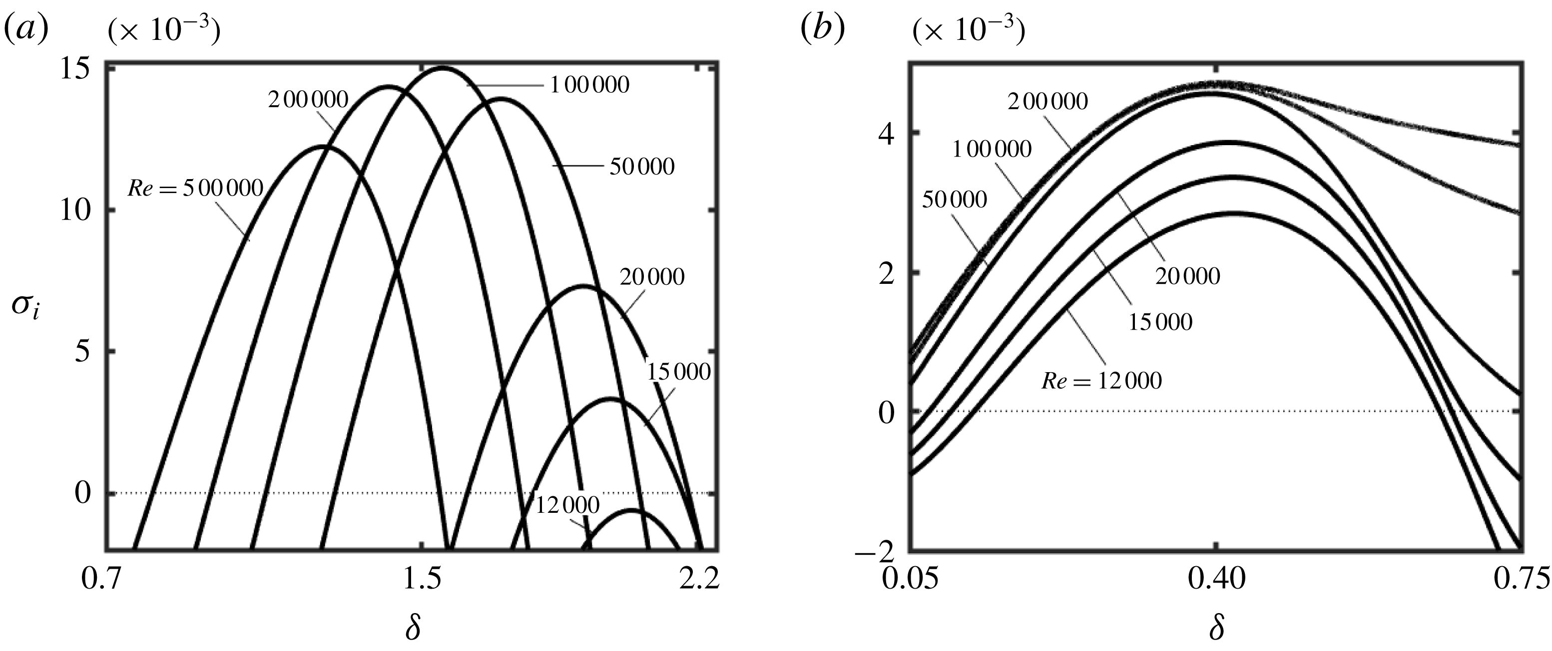
for the smallest
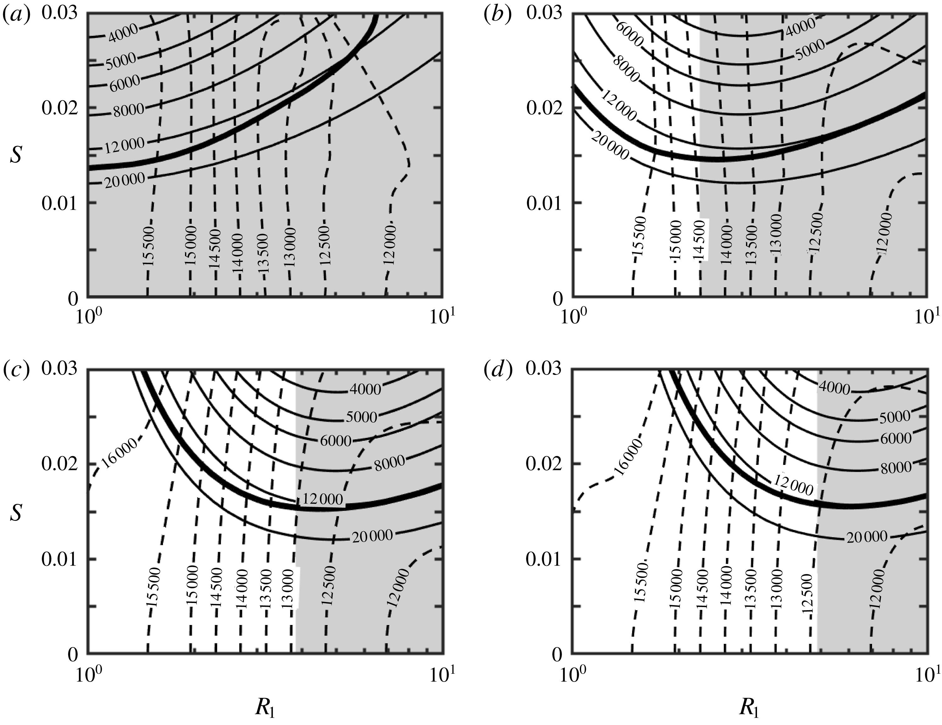
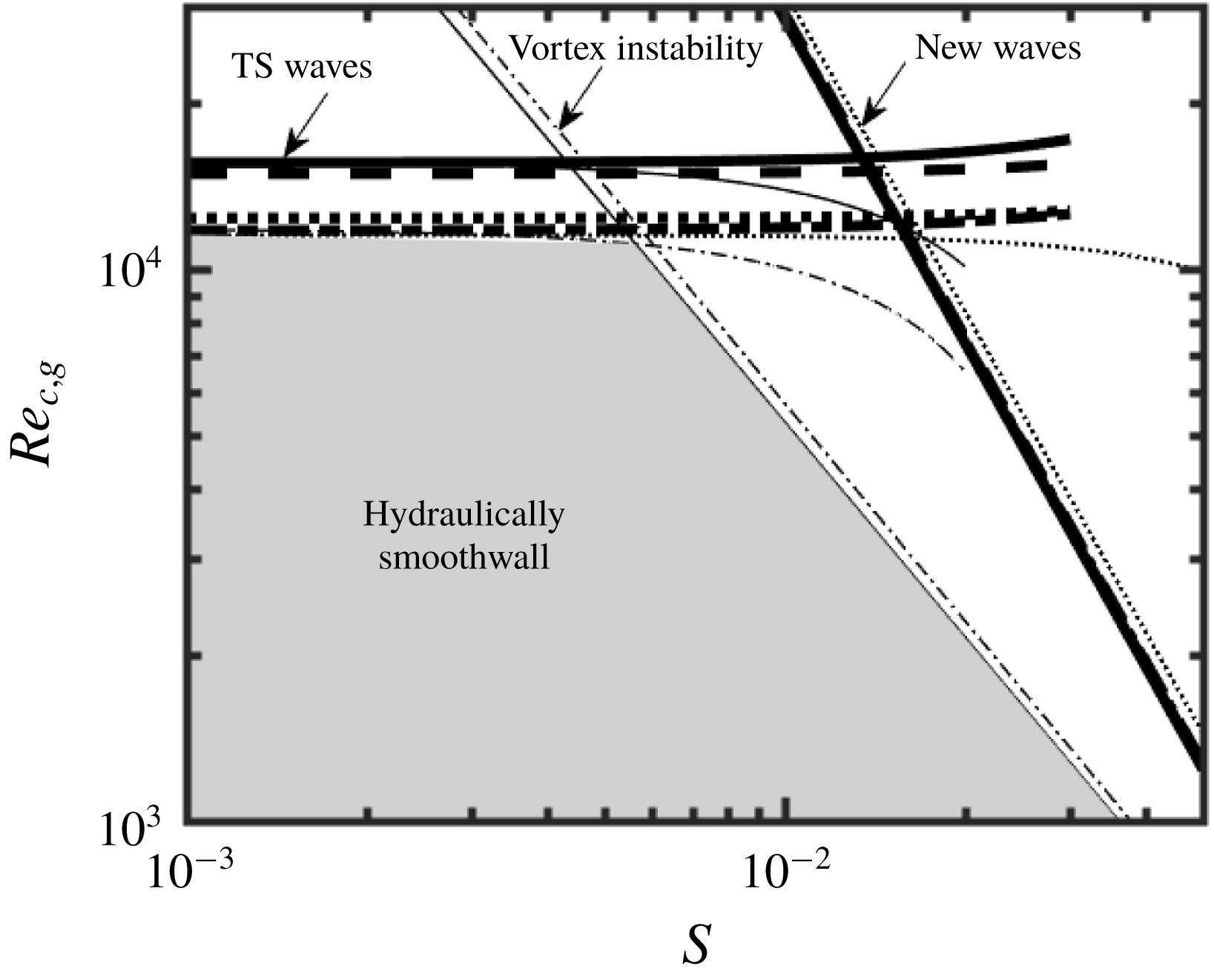
 $R_{1}$
considered (figure 29
a). The zone of their dominance expands towards larger
 $S$
when
 $R_{1}$
increases and thus grooves with larger amplitudes must be used to promote new waves (see figure 29
a). When five grooves are used
 $(M=5)$
, the smallest
 $S$
giving preference to the new waves is
 $S\approx 0.015$
but only if
 $R_{1}=3.2$
. Annuli with both smaller and larger radii require the use of taller grooves to give preference to the new waves (see figure 29
b). The pattern remains the same when eight grooves are used
 $(M=8)$
, with the most effective radius increasing to
 $R_{1}=5.3$
and the minimum
 $S$
capable of creating the new waves increasing to
 $S\approx 0.015$
(see figure 29
c). The same pattern is repeated for 10 grooves, as illustrated in figure 29(d).
Variations of the critical Reynolds number
 $Re_{c}$
as a function of
 $R_{1}$
and
 $S$
for the geometry described by (2.11). Results for
 $M=2$
, 5, 8 and 10 are displayed in (a–d), respectively. Solid and dashed lines correspond to the new waves and the TS waves, respectively. Thick lines separate zones of dominance of each type of waves. The shaded areas identify the drag-reducing configurations.

The selection of grooves provides a means for the development of passive flow control strategies with several distinct objectives. The first objective involves the laminar drag reduction and the data displayed in figures 2(a) and 29 provide information how much reduction can be achieved and the range of Reynolds numbers where these predictions are valid. The second objective involves the use of natural instabilities, like those described in this analysis, for the improvement of flow mixing with the smallest possible cost expressed in terms of the pressure gradient (Moradi & Floryan Reference Moradi and Floryan2013b
; Gepner & Floryan Reference Gepner and Floryan2016; Moradi et al.
Reference Moradi, Budiman and Floryan2017; Yadav et al.
Reference Yadav, Gepner and Szumbarski2017). Flows with small
 $Re$
are difficult to mix but the present results suggest that the new waves can be induced with quite small Reynolds numbers if tall enough grooves are used. The third objective is the control of the laminar–turbulent transition. Data displayed in figure 29 identify conditions when surface roughness in the form of longitudinal grooves can be ignored, as it does not lead to any instabilities. This determines some aspects of flow sensitivity with respect to geometric imperfections. When forcing of early transition is of interest, one can select a different set of grooves which would lead to the flow destabilization of interest.
4.6 Hydraulic smoothness
Grooves always affect the flow regardless of their amplitude and distribution. Small grooves are expected to produce only small flow changes but only if the system does not go through a bifurcation. Such grooves can be ignored, and the annulus can be viewed as being hydraulically smooth. The appearance of a secondary flow results in a qualitative change of the flow properties, as now small grooves produce large changes. This fact can be used to formulate a definition of the hydraulically smooth annuli following Floryan (Reference Floryan2007), i.e. the annulus is hydraulically smooth if surface corrugations are not able to create any system bifurcation. It should be stressed that this definition does not apply to turbulent flows where the concept of hydraulically smooth walls implies that the roughness elements are contained within the laminar sublayer. Data of the type presented in figure 29 can be used to identify configurations which do not create secondary flows. These conditions can be expressed using the global critical Reynolds number,
 $Re_{c,g}$
, defined as
 $$\begin{eqnarray}Re_{c,g}=\min _{\substack{ M \\ (R_{1},S=\text{const.})}}Re_{c},\end{eqnarray}$$
which corresponds to the minimum
 $Re_{c}$
over all
 $M$
values for a given
 $R_{1}$
and
 $S$
. This definition corresponds to practical applications where one typically measures roughness height and is less concerned with its spatial distribution (Morkovin Reference Morkovin, Hussaini and Voigt1990). Only
 $M<20$
were considered in the analysis and figure 30 illustrates the resulting variations of
 $Re_{c,g}$
as a function of the groove amplitude
 $S$
for a few typical radii. The ‘hydraulically smooth’ zone is bounded from above by the TS wave limitation, which is nearly independent of
 $S$
and shifts upwards as
 $R_{1}$
increases. This zone is bounded on the right side by the new wave limitation with
 $Re_{c,g}$
decreasing proportionally to
 $S^{-2}$
and being nearly independent of
 $R_{1}$
. Figure 30 displays data for the axisymmetric ribs (Moradi & Floryan Reference Moradi and Floryan2017b
). The TS limit is similar, but the right limit, which is determined by the centrifugal instability creating longitudinal vortices, is quite different. If one views axisymmetric ribs and longitudinal grooves as special limits of the two-dimensional roughness, i.e. spiral grooves, figure 30 identifies conditions when such roughness can be ignored regardless of the groove orientation.
Variations of the global critical Reynolds number
 $Re_{c,g}$
(see text for definition) as a function of the groove amplitude
 $S$
for the geometries described by (2.11). Solid, dashed, dotted and dash-dotted lines represent results for annuli with
 $R_{1}=1$
, 2, 5 and 10, respectively. Thin dotted lines represent the limit
 $R_{1}\rightarrow \infty$
(plane channel flow). The shaded area corresponds to configurations where the grooves are not able to induce any secondary flows. Thin lines represent results for annuli with axisymmetric ribs with
 $R_{1}=1$
(solid lines) and
 $R_{1}=10$
(dash-dotted lines).

4.7 Effects of groove shapes
The results discussed so far were obtained for grooves with sinusoidal shapes, e.g. (2.10). The problem formulation remains the same for arbitrary grooves as long as their shape can be described by a Fourier expansion, e.g. (2.1). It has been shown that the difference between hydrodynamic characteristics of a flow obtained by approximating the groove shape by its leading Fourier mode and the characteristics obtained with the full representation of the groove geometry are negligible in most applications (Floryan Reference Floryan2007). This conclusion, which applies to the drag analysis as well as to the stability analysis, forms the basis of the reduced geometry model which has been successfully applied in the analyses of several flows (Mohammadi & Floryan Reference Mohammadi and Floryan2013b ; Moradi & Floryan Reference Moradi and Floryan2013a , Reference Moradi and Floryan2014, Reference Moradi and Floryan2016b ; Moradi et al. Reference Moradi, Budiman and Floryan2017). The results presented in this paper provide therefore a good approximation of what can be achieved with grooves of arbitrary shape. One needs to measure the groove distribution, represent it using a Fourier expansion, identify the leading Fourier mode and extract flow characteristics corresponding to this mode from the data presented in the previous sections.
5 Conclusions
Laminar, pressure-driven flows in annuli made of two coaxial cylinders, with the inner cylinder modified by
 $M$
longitudinal grooves, were analysed. The analysis focused on grooves of sinusoidal shape, as their hydrodynamic properties well approximate the properties of grooves with arbitrary shapes (reduced-order geometry model) and was limited to grooves with amplitudes
 $S\leqslant 0.05$
. The primary flows were determined with spectral accuracy using the immersed boundary conditions (IBC) method to handle problems associated with the boundary irregularities. The onset conditions and the form of secondary flows were determined through the spectrally accurate solution of the linearized flow equations, with the IBC method used to handle the boundary conditions.
The primary flows have the circumferential structure dictated by the groove geometry. The analysis demonstrates the existence of surface topographies leading to the reduction of pressure losses while maintaining the same flow rate despite an increase of the wetted area of the inner cylinder. This effect is associated with the formation of high-velocity stream tubes in the widest annulus opening.
Conditions that guarantee the existence of primary states have been determined using linear stability theory. It was shown that two types of secondary flows emerge once the critical conditions are exceeded. Conditions giving preference to each of them were determined.
The first type of secondary flow has the form of classical travelling waves driven by shear (Tollmien–Schlichting (TS) waves) and modified by grooves. The presence of grooves increases the critical Reynolds number required for their onset. This can be explained by the overall reduction of shear in the case of drag-reducing configurations, and rearrangement of flow conditions in the vicinity of critical layers in the case of drag-increasing configurations. It was found that the axisymmetric waves dominate for sufficiently large radii of the annuli while different spiral waves dominate for small radii. The secondary flow topology is unique in the former case and has the form of axisymmetric rings propagating in the axial direction. The topologies in the latter case are not unique, as spiral waves with left and right twists can emerge under the same conditions, resulting in topologies varying from helical rings to rhombic structures. The most intense motion of this type occurs near the solid walls.
The second type of secondary flow has the form of travelling waves with characteristics very distinct from the TS waves. Its axisymmetric form dominates for all conditions considered in this analysis, with the most intense motion occurring near the gap centre and having a near-planar form concentrated in the circumferential and axial directions. It was shown that these waves are driven by inertial effects, that their critical Reynolds numbers change proportionally to
 $S^{-2}$
and thus that they can be significantly reduced if grooves of large enough amplitude are used. The relation between the onset conditions and the groove amplitude was established. Once activated, these waves always propagate with a phase speed near unity, which is approximately four times larger that the phase speed of the TS waves. Geometric parameters resulting in the minimum critical Reynolds number have also been identified. It was shown that the TS waves are dominant for small groove amplitude, i.e.
 $S\lesssim 0.01$
, and the new waves become dominant for larger amplitudes but within a well-defined range of radii of the annuli.
Longitudinal grooves represent a certain class of distributed surface roughness. The results presented in this paper can be used to assess how these grooves affect the initiation of the laminar–turbulent transition. Conditions when grooves do not create any instabilities regardless of their distribution have been determined. Surfaces with such grooves can be viewed as being hydraulically smooth.
The analysis is limited to asymptotic stability which is applicable to quiescent environments. Various bypass transition mechanisms are possible, but nothing is known about them in the context of annular flows. The noisy environment could give rise to transient growth scenarios which could be very complex in view of the existence of two types of instability waves documented in this paper. The present work should be viewed as providing foundations for analysis of more realistic situations where the flow is ‘contaminated’ by various non-negligible environmental disturbances, with the analysis of transient growth being the next logical step.
Acknowledgements
This work has been carried out with support from the Natural Sciences and Engineering Research Council (NSERC) of Canada.
Appendix A
Explicit expressions of the operators used in (3.15) and (3.16) have the form
 $$\begin{eqnarray}{\mathcal{L}}_{OS}^{(n)}=(-\text{i}\unicode[STIX]{x1D70E}+\text{i}\unicode[STIX]{x1D6FF}u_{z0}){\mathcal{T}}^{(n)}-\text{i}r\unicode[STIX]{x1D6FF}k_{n}^{2}\text{D}\left(\frac{\text{D}u_{z0}}{rk_{n}^{2}}\right)-\frac{1}{Re}{\mathcal{T}}^{(n)}{\mathcal{T}}^{(n)},\quad {\mathcal{C}}_{OS}^{(n)}=\frac{2\unicode[STIX]{x1D6FF}t_{n}}{Re}{\mathcal{T}}^{(n)},\end{eqnarray}$$
 $$\begin{eqnarray}{\mathcal{L}}_{SQ}^{(n)}=(-\text{i}\unicode[STIX]{x1D70E}+\text{i}\unicode[STIX]{x1D6FF}u_{z0})-\frac{{\mathcal{S}}^{(n)}}{Re},\quad {\mathcal{C}}_{SQ}^{(n)}=-\frac{\text{i}t_{n}\text{D}u_{z0}}{r^{3}k_{n}^{2}}-\frac{2\unicode[STIX]{x1D6FF}t_{n}}{r^{4}k_{(n)}^{4}Re}{\mathcal{T}}^{(n)},\end{eqnarray}$$
 $$\begin{eqnarray}{\mathcal{T}}^{(n)}=rk_{n}^{2}\text{D}\left(\frac{\text{D}}{rk_{n}^{2}}\right)-k_{n}^{2},\quad {\mathcal{S}}^{(n)}=\frac{1}{r^{3}k_{n}^{2}}\text{D}(r^{3}k_{n}^{2}\text{D})-k_{n}^{2},\end{eqnarray}$$
 $$\begin{eqnarray}\displaystyle {\mathcal{E}}_{v}^{(n,m)} & = & \displaystyle \text{i}\unicode[STIX]{x1D6FF}\left[k_{n}^{2}\,f^{(m)}-\left(\unicode[STIX]{x1D6FF}^{2}-\frac{t_{n}^{2}}{r^{2}}\right)\frac{\text{D}f^{(m)}}{rk_{n}^{2}}+\text{D}^{2}f^{(m)}\right]+\text{i}\unicode[STIX]{x1D6FF}\left\{\left[\unicode[STIX]{x1D6FF}^{2}-\frac{t_{n}^{2}}{r^{2}}-\frac{2mMt_{n-m}k_{n}^{2}}{r^{2}k_{n-m}^{2}}\right.\right.\nonumber\\ \displaystyle & & \displaystyle +\left.\left.\frac{4mM\unicode[STIX]{x1D6FF}^{2}t_{n-m}}{r^{2}k_{n-m}^{2}}\left(1+\frac{k_{n}^{2}}{k_{n-m}^{2}}\right)\right]\frac{f^{(m)}}{rk_{n}^{2}}-\frac{2mMt_{n-m}}{r^{2}k_{n-m}^{2}}\text{D}f^{(m)}\right\}\nonumber\\ \displaystyle & & \displaystyle -\,\text{i}\unicode[STIX]{x1D6FF}\left(1+\frac{2mMt_{n-m}}{r^{2}k_{n-m}^{2}}\right)f^{(m)}\text{D}^{2},\end{eqnarray}$$
 $$\begin{eqnarray}\displaystyle & \displaystyle {\mathcal{E}}_{\unicode[STIX]{x1D6FA}}^{(n,m)}=2\text{i}rmM\unicode[STIX]{x1D6FF}^{2}\left[\frac{2t_{n}^{2}}{r^{3}k_{n}^{2}}\,f^{(m)}+\text{D}f^{(m)}\right]+2\text{i}rmM\unicode[STIX]{x1D6FF}^{2}f^{(m)}\text{D}, & \displaystyle\end{eqnarray}$$
 $$\begin{eqnarray}\displaystyle & \displaystyle {\mathcal{F}}_{v}^{(n,m)}=\text{i}t_{n}\frac{\text{D}f^{(m)}}{r^{3}k_{n}^{2}}-\text{i}mM\left(1+\frac{mMt_{n-m}}{r^{2}k_{n-m}^{2}}\right)\frac{f^{(m)}}{r^{3}k_{n}^{2}}\text{D}, & \displaystyle\end{eqnarray}$$
 $$\begin{eqnarray}\displaystyle & \displaystyle {\mathcal{F}}_{\unicode[STIX]{x1D6FA}}^{(n,m)}=-\text{i}\unicode[STIX]{x1D6FF}\left(\frac{k_{n-m}^{2}}{k_{n}^{2}}-\frac{m^{2}M^{2}}{r^{2}k_{n}^{2}}\right)f^{(m)}, & \displaystyle\end{eqnarray}$$
where
 $t_{n-m}=(n-m)M+\unicode[STIX]{x1D6EC}$
,
 $k_{n-m}^{2}=\unicode[STIX]{x1D6FF}^{2}+t_{n-m}^{2}/r^{2}$
and
 $\text{D}^{n}=\text{d}^{n}/\text{d}r^{n}$
.
Appendix B
The flow domain is confined between
 $R_{1}-R_{in}$
and
 $1+R_{1}$
, where
 $R_{in}$
denotes the location of the lower groove extremity. This domain is mapped into
 $(-1,1)$
using the transformation of the form
 $$\begin{eqnarray}\hat{r}=[r-(1+R_{1})]\unicode[STIX]{x1D6E4}+1,\quad \unicode[STIX]{x1D6E4}=2(1+R_{in})^{-1}\end{eqnarray}$$
to permit the use of the standard form of Chebyshev polynomials. The homogeneous boundary conditions (3.6) expressed in terms of
 $G_{v}^{(n)}(r)$
and
 $\unicode[STIX]{x1D6FA}^{(n)}(r)$
have the following forms:
 $$\begin{eqnarray}\displaystyle & \displaystyle u_{rD}(\hat{r},\unicode[STIX]{x1D703},z,t)=\mathop{\sum }_{n=-N_{N}}^{N_{N}}\frac{\text{i}G_{v}^{(n)}(\hat{r})}{f(\hat{r})}\text{e}^{\text{i}[\unicode[STIX]{x1D6FF}z+(\unicode[STIX]{x1D6EC}+nM)\unicode[STIX]{x1D703}-\unicode[STIX]{x1D70E}t]}=0, & \displaystyle\end{eqnarray}$$
 $$\begin{eqnarray}\displaystyle & \displaystyle u_{\unicode[STIX]{x1D703}D}(\hat{r},\unicode[STIX]{x1D703},z,t)=\mathop{\sum }_{n=-N_{N}}^{N_{N}}\left[-\frac{t_{n}\text{D}G_{v}^{(n)}(\hat{r})}{f^{2}(\hat{r})\hat{k}_{n}^{2}}+\unicode[STIX]{x1D6FF}f(\hat{r})\unicode[STIX]{x1D6FA}^{(n)}(\hat{r})\right]\text{e}^{\text{i}[\unicode[STIX]{x1D6FF}z+(\unicode[STIX]{x1D6EC}+nM)\unicode[STIX]{x1D703}-\unicode[STIX]{x1D70E}t]}=0, & \displaystyle\end{eqnarray}$$
 $$\begin{eqnarray}\displaystyle & \displaystyle u_{zD}(\hat{r},\unicode[STIX]{x1D703},z,t)=\mathop{\sum }_{n=-N_{N}}^{N_{N}}\left[-\frac{\unicode[STIX]{x1D6FF}\text{D}G_{v}^{(n)}(\hat{r})}{f(\hat{r})\hat{k}_{n}^{2}}-t_{n}\unicode[STIX]{x1D6FA}^{(n)}(\hat{r})\right]\text{e}^{\text{i}[\unicode[STIX]{x1D6FF}z+(\unicode[STIX]{x1D6EC}+nM)\unicode[STIX]{x1D703}-\unicode[STIX]{x1D70E}t]}=0, & \displaystyle\end{eqnarray}$$
where
 $f(\hat{r})=\unicode[STIX]{x1D6E4}^{-1}(\hat{r}-1)+1+R_{1}$
and
 $\hat{k}_{n}^{2}=\unicode[STIX]{x1D6FF}^{2}+f^{-2}(\hat{r})t_{n}^{2}$
. The location of the inner cylinder in the
 $(\hat{r},\unicode[STIX]{x1D703})$
coordinate system is given as
 $$\begin{eqnarray}\hat{r}_{in}(\unicode[STIX]{x1D703})=\mathop{\sum }_{n=-N_{A}}^{N_{A}}A^{(n)}\text{e}^{\text{i}nM\unicode[STIX]{x1D703}},\end{eqnarray}$$
where
 $A^{(n)}=1-\unicode[STIX]{x1D6E4}+\unicode[STIX]{x1D6E4}H^{(n)}$
for
 $n=0$
and
 $A^{(n)}=\unicode[STIX]{x1D6E4}H^{(n)}$
for
 $n\neq 0$
. As the first step, consider boundary condition (B 4). Substitution of (3.19) into (B 4) leads to
 $$\begin{eqnarray}\mathop{\sum }_{n=-N_{N}}^{N_{N}}\mathop{\sum }_{k=0}^{N_{C}}\left\{-\frac{\unicode[STIX]{x1D6E4}\unicode[STIX]{x1D6FF}\text{D}T_{k}[\hat{r}_{in}(\unicode[STIX]{x1D703})]}{f(\hat{r})\hat{k}_{n}^{2}}G_{k,v}^{(n)}-t_{n}T_{k}[\hat{r}_{in}(\unicode[STIX]{x1D703})]G_{k,\unicode[STIX]{x1D6FA}}^{(n)}\right\}\text{e}^{\text{i}[\unicode[STIX]{x1D6FF}z+(\unicode[STIX]{x1D6EC}+nM)\unicode[STIX]{x1D703}-\unicode[STIX]{x1D70E}t]}=0.\end{eqnarray}$$
Values of the Chebyshev polynomials and their first derivatives evaluated along the inner cylinder appearing in the above relation, i.e.
 $T_{k}[\hat{r}_{in}(\unicode[STIX]{x1D703})]$
and
 $\text{D}T_{k}[\hat{r}_{in}(\unicode[STIX]{x1D703})]$
, represent periodic functions of
 $\unicode[STIX]{x1D703}$
and thus can be expressed using Fourier expansions of the form
 $$\begin{eqnarray}T_{k}[\hat{r}_{in}(\unicode[STIX]{x1D703})]=\mathop{\sum }_{m=-N_{S}}^{N_{S}}w_{k}^{(m)}\text{e}^{\text{i}mM\unicode[STIX]{x1D703}},\quad \text{D}T_{k}[\hat{r}_{in}(\unicode[STIX]{x1D703})]=\mathop{\sum }_{m=-N_{S}}^{N_{S}}d_{k}^{(m)}\text{e}^{\text{i}mM\unicode[STIX]{x1D703}},\end{eqnarray}$$
where
 $N_{S}=N_{A}N_{C}$
. Evaluation of coefficients
 $w_{k}^{(m)}$
begins with the lowest-order Chebyshev polynomial, i.e.
 $$\begin{eqnarray}\left.\begin{array}{@{}c@{}}\displaystyle \!\!\!T_{0}=1~\Rightarrow \mathop{\sum }_{m=-N_{S}}^{N_{S}}w_{0}^{(m)}\text{e}^{\text{i}mM\unicode[STIX]{x1D703}}=1~\Rightarrow ~w_{0}^{(0)}=1\;\text{for }m=0\;\text{and}\;w_{0}^{(m)}=0\;\text{for }m\neq 0,\\ \displaystyle T_{1}[\hat{r}_{in}(\unicode[STIX]{x1D703})]=\hat{r}_{in}(\unicode[STIX]{x1D703})~\Rightarrow ~\mathop{\sum }_{m=-N_{S}}^{N_{S}}w_{1}^{(m)}\text{e}^{\text{i}mM\unicode[STIX]{x1D703}}=\mathop{\sum }_{m=-\infty }^{\infty }A^{(m)}\text{e}^{\text{i}mM\unicode[STIX]{x1D703}}~\Rightarrow ~w_{1}^{(m)}=A^{(m)}.\end{array}\right\}\end{eqnarray}$$
The remaining coefficients
 $w_{k}^{(m)}\,(k\geqslant 2)$
can be computed using the Chebyshev recursion relation, which results in
 $$\begin{eqnarray}w_{k+1}^{(m)}=2\mathop{\sum }_{n=-N_{A}}^{N_{A}}A^{(n)}w_{k}^{(m-n)}-w_{k-1}^{(m)},\quad k\geqslant 2.\end{eqnarray}$$
Evaluation of the coefficients
 $d_{k}^{(m)}$
also begins with the lowest-order polynomial, i.e.
 $$\begin{eqnarray}\left.\begin{array}{@{}c@{}}\displaystyle \text{D}T_{0}=0~\Rightarrow ~\mathop{\sum }_{m=-N_{S}}^{N_{S}}d_{0}^{(m)}\text{e}^{\text{i}mM\unicode[STIX]{x1D703}}=0~\Rightarrow ~d_{0}^{(0)}=0,\\ \displaystyle \text{D}T_{1}=1~\Rightarrow ~\mathop{\sum }_{m=-N_{S}}^{N_{S}}d_{0}^{(m)}\text{e}^{\text{i}mM\unicode[STIX]{x1D703}}=1~\Rightarrow ~d_{0}^{(0)}=1\;\text{for }m=0,\quad d_{0}^{(m)}=0,\;\text{for }m\neq 0,\\ \displaystyle \text{D}T_{2}[\hat{r}_{in}(\unicode[STIX]{x1D703})]=4\hat{r}_{in}(\unicode[STIX]{x1D703})~\Rightarrow ~\mathop{\sum }_{m=-N_{S}}^{N_{S}}d_{2}^{(m)}\text{e}^{\text{i}mM\unicode[STIX]{x1D703}}=\mathop{\sum }_{m=-\infty }^{\infty }4A^{(m)}\text{e}^{\text{i}mM\unicode[STIX]{x1D703}}~\Rightarrow ~d_{2}^{(m)}=4A^{(m)}.\end{array}\right\}\end{eqnarray}$$
The remaining coefficients
 $d_{k}^{(m)},~k\geqslant 3$
, can be computed using the Chebyshev recursive formula and have the following form:
 $$\begin{eqnarray}d_{k+1}^{(m)}=2\mathop{\sum }_{n=-N_{A}}^{N_{A}}A^{(n)}d_{k}^{(m-n)}-d_{k-1}^{(m)}-w_{k}^{(m)},\quad k\geqslant 3.\end{eqnarray}$$
Substitution of (B 7) into (B 6) leads to a boundary relation of the form
 $$\begin{eqnarray}\mathop{\sum }_{-N_{N}-N_{S}}^{N_{N}+N_{S}}\mathop{\sum }_{m=-N_{N}}^{N_{N}}\mathop{\sum }_{k=0}^{N_{C}}\left\{-\frac{\unicode[STIX]{x1D6E4}\unicode[STIX]{x1D6FF}d_{k}^{(n-m)}}{f(\hat{r})\hat{k}_{m}^{2}}G_{k,v}^{(m)}-t_{m}w_{k}^{(n-m)}G_{k,\unicode[STIX]{x1D6FA}}^{(m)}\right\}\text{e}^{\text{i}[\unicode[STIX]{x1D6FF}z+(\unicode[STIX]{x1D6E4}+nM)\unicode[STIX]{x1D703}-\unicode[STIX]{x1D70E}t]}=0.\end{eqnarray}$$
The function
 $1/f(\hat{r})\hat{k}_{m}^{2}$
evaluated along the inner cylinder represents a periodic function of
 $\unicode[STIX]{x1D703}$
and can be expressed in terms of the Fourier expansion of the form
 $$\begin{eqnarray}\frac{1}{f(\hat{r})\hat{k}_{m}^{2}}=\mathop{\sum }_{p=-N_{R}}^{N_{R}}F_{u,m}^{(p)}\text{e}^{\text{i}pM\unicode[STIX]{x1D703}},\end{eqnarray}$$
where the Fourier coefficients
 $F_{u,m}^{(p)}$
can be computed for each mode
 $m$
using the fast Fourier transform (FFT) algorithm. The
 $N_{R}$
value depends on the complexity of the geometry and for simple cosine shape
 $N_{R}=N_{N}$
provides machine-level accuracy. Substitution of (B 13) into (B 12) and separation for Fourier modes results in the final form of the boundary condition for
 $u_{zD}$
suitable for numerical implementation, i.e.
 $$\begin{eqnarray}\mathop{\sum }_{m=-N_{N}}^{N_{N}}\mathop{\sum }_{k=0}^{N_{C}}\unicode[STIX]{x1D6E4}\unicode[STIX]{x1D6FF}G_{k,v}^{(m)}\mathop{\sum }_{p=-N_{N}-N_{S}}^{N_{N}+N_{S}}F_{u,m}^{(n-p)}d_{k}^{(p-m)}+\mathop{\sum }_{m=-N_{N}}^{N_{N}}\mathop{\sum }_{k=0}^{N_{C}}t_{m}w_{k}^{(n-m)}G_{k,\unicode[STIX]{x1D6FA}}^{(m)}=0.\end{eqnarray}$$
Following the same procedure, the boundary constraints for
 $u_{rD}$
and
 $u_{\unicode[STIX]{x1D703}D}$
can be written in the form
 $$\begin{eqnarray}\mathop{\sum }_{m=-N_{N}}^{N_{N}}\mathop{\sum }_{k=0}^{N_{C}}G_{k,v}^{(m)}\mathop{\sum }_{p=-N_{N}-N_{S}}^{N_{N}+N_{S}}F_{v}^{(n-p)}w_{k}^{(p-m)}=0\end{eqnarray}$$
and
 $$\begin{eqnarray}\displaystyle & & \displaystyle -\mathop{\sum }_{m=-N_{N}}^{N_{N}}\mathop{\sum }_{k=0}^{N_{C}}\unicode[STIX]{x1D6E4}t_{m}G_{k,v}^{(m)}\mathop{\sum }_{p=-N_{N}-N_{S}}^{N_{N}+N_{S}}F_{w,m}^{(n-p)}d_{k}^{(p-m)}\nonumber\\ \displaystyle & & \displaystyle \quad +\,\mathop{\sum }_{m=-N_{N}}^{N_{N}}\mathop{\sum }_{k=0}^{N_{C}}\unicode[STIX]{x1D6FF}G_{k,\unicode[STIX]{x1D6FA}}^{(m)}\mathop{\sum }_{p=-N_{N}-N_{S}}^{N_{N}+N_{S}}F_{f}^{(n-p)}w_{k}^{(p-m)}=0,\end{eqnarray}$$
where
 $$\begin{eqnarray}\frac{1}{f[\hat{r}_{in}(\unicode[STIX]{x1D703})]}=\mathop{\sum }_{p=-N_{R}}^{N_{R}}F_{v}^{(p)}\text{e}^{\text{i}pM\unicode[STIX]{x1D703}},\quad \frac{1}{f^{2}[\hat{r}_{in}(\unicode[STIX]{x1D703})]\hat{k}_{m}^{2}}=\mathop{\sum }_{p=-N_{R}}^{N_{R}}F_{w,m}^{(p)}\text{e}^{\text{i}pM\unicode[STIX]{x1D703}},\end{eqnarray}$$
and
 $F_{f}^{(p)}=R_{1}+H^{(p)}$
for
 $p=0$
and
 $F_{f}^{(p)}=H^{(p)}$
for
 $p\neq 0$
.
Since the outer cylinder is smooth, the discretized boundary conditions there have simple forms, i.e.
 $$\begin{eqnarray}\displaystyle & \displaystyle \mathop{\sum }_{k=0}^{N_{C}}\frac{\text{i}G_{k,v}^{(m)}}{1+R_{1}}=0, & \displaystyle\end{eqnarray}$$
 $$\begin{eqnarray}\displaystyle & \displaystyle \mathop{\sum }_{k=0}^{N_{C}}\left[-\frac{\unicode[STIX]{x1D6E4}t_{m}k^{2}}{(1+R_{1})^{2}\unicode[STIX]{x1D6FF}^{2}+t_{m}^{2}}G_{k,v}^{(m)}+\unicode[STIX]{x1D6FF}(1+R_{1})G_{k,\unicode[STIX]{x1D6FA}}^{(m)}\right]=0, & \displaystyle\end{eqnarray}$$
 $$\begin{eqnarray}\displaystyle & \displaystyle \mathop{\sum }_{k=0}^{N_{C}}\left[\frac{\unicode[STIX]{x1D6E4}\unicode[STIX]{x1D6FF}(1+R_{1})k^{2}}{(1+R_{1})^{2}\unicode[STIX]{x1D6FF}^{2}+t_{m}^{2}}G_{k,v}^{(m)}+t_{m}G_{k,\unicode[STIX]{x1D6FA}}^{(m)}\right]=0. & \displaystyle\end{eqnarray}$$
The reader may note that the boundary constraints at the inner cylinder provide coupling between different Fourier modes.