1 Introduction
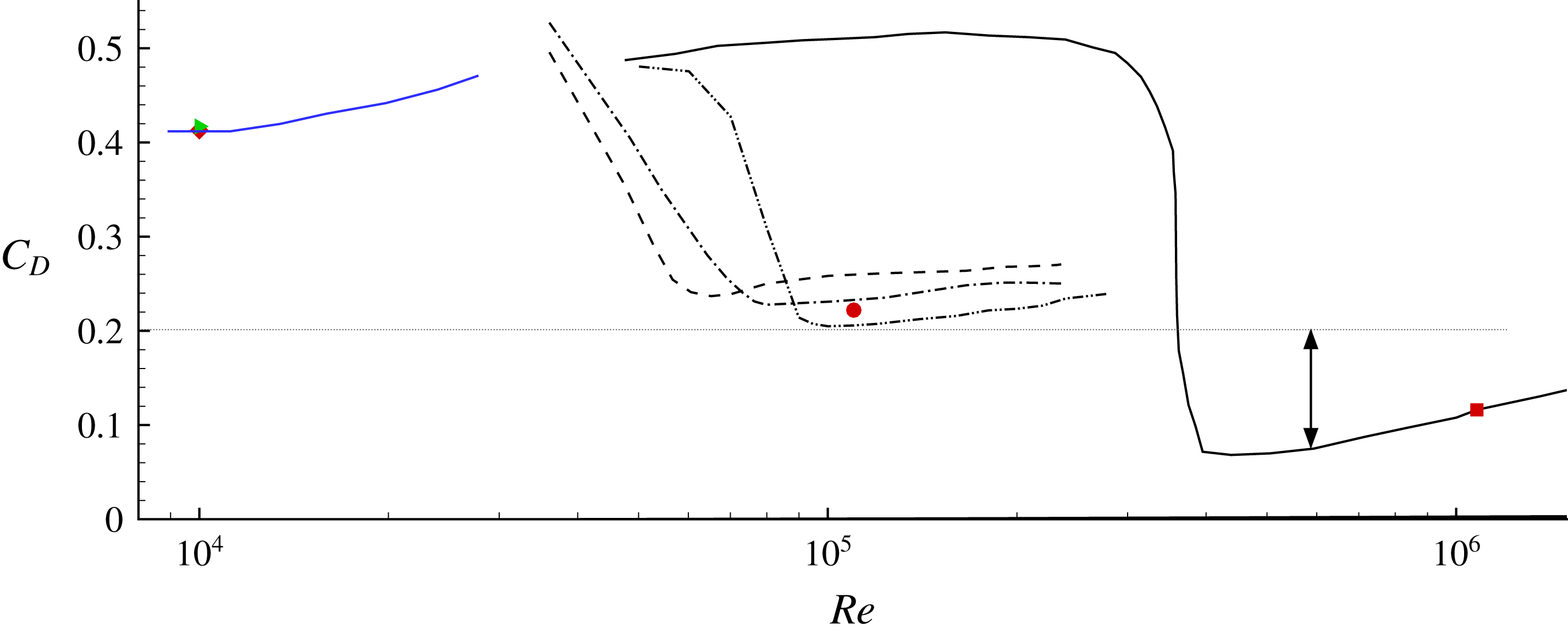
Passive roughness elements, such as trip wires, dimples, sand-grain roughness, etc., are effective in reducing the drag force on bluff (i.e. sphere, cylinder) as well as streamlined (i.e. airfoils) bodies (see Choi, Jeon & Kim Reference Choi, Jeon and Kim2008, for a review). Among the different types of elements, dimples are very efficient in maintaining the low drag configuration for a large range of Reynolds numbers. An example is shown in figure 1, where the variation of the drag coefficient
 $C_{D}=2F_{D}/\unicode[STIX]{x1D70C}{U_{\infty }}^{2}A$
as a function of Reynolds number
 $Re=U_{\infty }D/\unicode[STIX]{x1D708}$
(here
 $F_{D}$
is the drag force,
 $U_{\infty }$
is the free-stream velocity,
 $D$
the sphere diameter,
 $A$
the reference area, and
 $\unicode[STIX]{x1D70C}$
and
 $\unicode[STIX]{x1D708}$
the density and kinematic viscosity of the fluid, respectively) is plotted for smooth and dimpled spheres. For the former case, the drag coefficient remains constant (
 $C_{D}\sim 0.5$
) until the Reynolds number approaches a critical value (
 $Re\sim 3\times 10^{5}$
). At this point, which is usually referred to as the drag crisis,
 $C_{D}$
decreases rapidly and hits a minimum, which is an order of magnitude lower (
 $C_{D}\sim 0.08$
). With further increase in the Reynolds number, the flow enters into the post-critical regime characterized by turbulent boundary layers on the surface of the sphere. In this regime the drag coefficient rises slowly with increasing Reynolds number.
Drag coefficient as a function of the Reynolds number for various spheres: black ——, smooth sphere, Achenbach (Reference Achenbach1972); blue ——, smooth sphere, Wieselsberger (Reference Wieselsberger1922); — ⋅ ⋅ —, dimpled sphere, Choi, Jeon & Choi (Reference Choi, Jeon and Choi2006); - - - -, dimpled sphere with spherical dimples, Bearman & Harvey (Reference Bearman and Harvey1976); — ⋅ —, dimpled sphere with hexagonal dimples, Bearman & Harvey (Reference Bearman and Harvey1976); ▸, dimpled sphere at
 $Re=10\,000$
, present direct numerical simulation (DNS); ♦, smooth sphere at
 $Re=10\,000$
, present DNS; ●, dimpled sphere at
 $Re=110\,000$
, present DNS.

In dimpled spheres the drag crisis happens at a much lower critical Reynolds number (
 $Re<7\times 10^{4}$
in figure 1). The critical value of the Reynolds number as well as the attained minimum drag coefficient in the post-critical regime depend on the dimple geometry and arrangement. One of the earliest studies on golf ball aerodynamics was carried out by Bearman & Harvey (Reference Bearman and Harvey1976), where a series of wind tunnel tests on stationary and spinning dimpled spheres were reported. They found that hexagonal dimples shift the drag crisis at a slightly higher Reynolds number and result in a lower drag coefficient when compared to spherical dimples for both stationary and spinning configurations. Their study only reported forces and did not provide information on the flow. They conjectured, however, that this behaviour was due to the fact that hexagonal dimples are more efficient trips than round dimples, perhaps by shedding more vortices from their straight edges into the boundary layer.
Choi et al. (Reference Choi, Jeon and Choi2006) carried out wind tunnel experiments on stationary dimpled spheres and focused on the effects of the Reynolds number on the flow. They used surface oil flow visualization to identify the global separation line and measured the streamwise velocity inside and around the dimples. Their measurements, for the first time, provided a glimpse on the complexity of near-wall flow and its impact on global separation. In particular, they found that dimples cause local flow separation, leading to the formation of a detached shear layer that becomes unstable, resulting in the generation of turbulence, which causes transport of high-speed fluid closer to the wall. They also showed that, as the Reynolds number is increased, the transition point moves gradually upstream but the global separation point remains unchanged. The latter is consistent with the observation that the drag coefficient remains almost constant after the drag crisis.
Aoki et al. (Reference Aoki, Ohike, Yamaguchi and Nakayama2003, Reference Aoki, Muto, Okanaga and Nakayama2009) and Aoki, Muto & Okanaga (Reference Aoki, Muto and Okanaga2012) reported experiments on dimpled spheres where they studied the effects of dimple depth and dimple coverage on the drag coefficient. In one of their experiments (Aoki et al. Reference Aoki, Muto, Okanaga and Nakayama2009) they used a pressure transducer to measure the pressure at selected points inside and outside of the dimples. The approximate location of the global separation line was then determined based on the pressure recovery. They showed that, as the dimple depth increased, the separation line moved upstream, which is consistent with the increased drag coefficient they reported. In another series of experiments (Aoki et al. Reference Aoki, Ohike, Yamaguchi and Nakayama2003) they measured the location of the separation line using an oil film method and showed that, as the dimple coverage increased, global separation was further delayed but the drag coefficient increased. This finding may seem counterintuitive and clearly demonstrates that the location of the global separation alone is not enough to explain the behaviour of the drag coefficient on dimpled spheres.
Overall the above studies indicate that the dimple topology has an impact on the critical Reynolds number, as well as the minimum attained drag coefficient. In general, as the dimple depth or the number of dimples is increased, the drag crisis is accelerated and the drag coefficient in the post-critical regime increases. However, in all the above studies the minimum value of the drag coefficient is above
 $C_{D}\sim 0.2$
, which is two to three times higher than the value observed for a smooth sphere in the post-critical regime. This is a significant difference and it is usually attributed to differences in global separation, while dimples, much like sand-grain roughness, are considered to have a small contribution towards the friction drag. Smits & Ogg (Reference Smits and Ogg2004), for example, speculated that increasing the dimple depth will increase the overall drag by primarily increasing the skin fiction. However, there are no quantitative results to support this conjecture and the origin of the drag force on dimpled spheres is still an open question. Addressing this question is critical to better understand the drag penalty on dimpled surfaces.
Given that experiments have limitations to measure the flow within the dimples with enough resolution to determine the pressure and friction portions of the total drag force, high-fidelity computations are the primary tool able to address the above questions.
In the present study we report a direct numerical simulation (DNS) of a dimpled sphere at post-critical Reynolds numbers. The flow near the dimpled surface as well as the wake is resolved at an unprecedented level of detail using billions of grid nodes. Our main objective is to establish an understanding of the relation between drag reduction induced by dimples and the penalties originating from the dimples themselves. The results presented in this paper challenge the broadly accepted view that the dimples only indirectly affect the drag force by manipulating the structure of the turbulent boundary layer near the wall and consequently affect global separation. The DNS reveal that the penalty on the drag force due to the dimples is very significant (as much as
 $60\,\%$
of the total drag force) and it is primarily pressure drag. The methodologies and details of the computations will be given in the next section, followed by the results and conclusions.
2 Methodologies and set-up
The Navier–Stokes equations for viscous incompressible flow are solved on a structured grid in cylindrical coordinates. The letters
 $r$
,
 $\unicode[STIX]{x1D719}$
and
 $z$
denote the radial, azimuthal and axial coordinates, respectively, while
 $\unicode[STIX]{x1D703}$
denotes the polar angle, going from
 $0^{\circ }$
at the stagnation point at the front of the sphere to
 $180^{\circ }$
at the wake side. The governing equations are advanced in time using a semi-implicit projection method, treating the explicit part with a third-order Runge–Kutta scheme, and the implicit part with a second-order Crank–Nicolson scheme. All spatial derivatives are discretized using second-order central differences on a staggered grid. To overcome the severe time-step limitation imposed by the nature of the cylindrical coordinate grid, the viscous and convective terms are treated implicitly in the azimuthal direction, near the centreline, and in the radial direction, near the top of the sphere. The pressure Poisson equation, which enables the projection of the predicted velocity into a divergence-free field, is solved using a direct solver. The heptadiagonal matrix is initially reduced to a series of pentadiagonal problems via fast Fourier transforms (FFTs) along the periodic direction, which are then solved with a divide-and-conquer strategy (see Toivanen & Rossi Reference Toivanen and Rossi2001). The code is parallelized using a domain decomposition approach in the streamwise direction, where all communication between processors is handled utilizing Message Passing Interface (MPI) library calls.
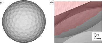
The geometry of the smooth or dimpled sphere is represented by a Lagrangian grid consisting of triangular elements (see figure 2 b). The requirement for the Eulerian grid to conform to the body is relaxed, and the non-slip boundary conditions are imposed using the immersed-boundary formulation proposed by Balaras (Reference Balaras2004) and Yang & Balaras (Reference Yang and Balaras2006). The overall method can be summarized in the following steps. (i) All computational points on the fixed Eulerian grid are classified according to their relation with the solid body using a ray-tracing technique. They all fall into three categories: solid (the ones overlapping with the solid body), fluid (the ones outside the solid body) and forcing (all fluid points that have at least one neighbour in the solid). (ii) The velocity field at the forcing nodes is reconstructed in order to satisfy the boundary conditions on the solid body. Details on our implementation within the framework of the fractional step scheme discussed above can be found in Balaras (Reference Balaras2004) and Yang & Balaras (Reference Yang and Balaras2006). The resulting formulation is second-order-accurate in both space and time. An extensive validation on practical flow problems over a wide range of Reynolds numbers can be found in Posa et al. (Reference Posa, Lippolis, Verzicco and Balaras2011), Balaras, Schroeder & Posa (Reference Balaras, Schroeder and Posa2015), Posa, Lippolis & Balaras (Reference Posa, Lippolis and Balaras2015), Posa & Balaras (Reference Posa and Balaras2016), Rahromostaqim, Posa & Balaras (Reference Rahromostaqim, Posa and Balaras2016), Pal et al. (Reference Pal, Sarkar, Posa and Balaras2017) and Posa & Balaras (Reference Posa and Balaras2018).
(a) Dimpled sphere representative of a commercial golf ball with 312 spherical dimples. (b) Fixed Eulerian grid at a plane going through the dimple. The triangular elements representing the surface of the dimpled sphere (Lagrangian grid) are also visible.

Figure 2 shows the geometry of the dimpled sphere used in this study. It contains
 $312$
spherical dimples, with an average diameter
 $d=0.095D$
and maximum depth
 $k=0.0067D$
. The resulting dimple coverage, which is the ratio of the surface area occupied by the dimples to the total surface of a sphere, is approximately
 $70\,\%$
. The geometry is representative of a commercial golf ball. We report DNS at two flow regimes: (i) Subcritical at
 $Re=1.0\times 10^{4}$
, where the dimples do not cause a drag crisis, and there is no dramatic reduction in the drag coefficient when compared to that of a smooth sphere; for this case we also computed the flow around a smooth sphere to facilitate comparisons. (ii) Post-critical at
 $Re=1.1\times 10^{5}$
, where a dramatic reduction in the drag coefficient is observed compared to a smooth sphere due to the presence of the dimples; note that for this case the experimental results by Achenbach (Reference Achenbach1972) are used for comparisons due to cost considerations.
For all cases the computational domain extends
 $10D$
upstream and
 $30D$
downstream of the sphere (the centre of the sphere is located at
 $r/D=0$
,
 $z/D=0$
). At the inlet a uniform velocity profile is specified, and at the outflow the convective boundary condition proposed by Orlanski (Reference Orlanski1976) is used. The latter utilizes the one-dimensional wave equation at the outflow boundary to convect all the eddies out of the computational box. In our implementation the grid spacing in the axial direction for the last one-third of the domain is rapidly increased to prevent any residual disturbances from travelling upstream. A series of computations for subcritical conditions where the outflow boundary was placed at
 $20D$
,
 $30D$
and
 $50D$
(not shown here) enabled us to select the present computational box as optimal. In the azimuthal direction, periodic boundary condition are used, while at the free-stream boundary a free-slip condition is enforced. For the subcritical case (
 $Re=1.0\times 10^{4}$
) the grid involved
 $510\times 302\times 752$
nodes in the radial, azimuthal and streamwise directions, respectively, while for the post-critical case (
 $Re=1.1\times 10^{5}$
) it involved
 $1100\times 1502\times 3002$
. In both cases the computational grid is stretched in the axial and radial directions to resolve the key flow features.
An example of the grid structure near a dimple is shown in figure 2(b). Typical grid resolution for a dimple at approximately
 $90^{\circ }$
from the stagnation point utilizes
 $40$
points along its depth,
 $70$
points in the streamwise and
 $50$
points in the spanwise directions, respectively. For the post-critical case, where part of the boundary layer on the surface of the dimpled sphere is turbulent, one can also estimate the grid resolution in wall units,
 $\unicode[STIX]{x0394}x^{+}=\unicode[STIX]{x0394}xu_{\unicode[STIX]{x1D70F}}/\unicode[STIX]{x1D708}$
(where
 $u_{\unicode[STIX]{x1D70F}}$
is the wall shear velocity and
 $\unicode[STIX]{x1D708}$
is the kinematic viscosity). Since
 $u_{\unicode[STIX]{x1D70F}}$
varies on the surface, we utilize an average value at
 $\unicode[STIX]{x1D703}=90^{\circ }$
, where it reaches its maximum value. Using this value the grid resolution in the wall-normal direction
 $\unicode[STIX]{x0394}r^{+}\sim 1.0$
, while
 $\unicode[STIX]{x0394}\unicode[STIX]{x1D719}^{+}\sim 10.0$
and
 $\unicode[STIX]{x0394}z^{+}\sim 8.0$
.
Owing to cost considerations (the above grid already utilizes close to five billion nodes), the sensitivity of the results to grid resolution was established on a reduced configuration, which captures the critical flow features of the full configuration. In particular, we considered a narrow section of a half-cylinder. The surface of the half-cylinder was covered with the same dimples as above and the Reynolds number was set to
 $Re_{D}=160\,000$
to ensure we fall into the post-critical regime. Three grids with progressively
 $50\,\%$
more points in each direction were used: coarse, medium and fine. The resolution of the medium grid is equivalent to the resolution utilized in the dimpled sphere computations reported below. The pressure and skin friction coefficients for the medium and fine grids on the half-cylinder configuration were identical (within
 $2\,\%$
), while differences of up to
 $10\,\%$
were present for the coarsest grid. This result gives us confidence that the grid utilized above is adequate.
To minimize transients the computations were started on coarser grids and were gradually transferred onto finer ones until the final resolution was reached. Approximately
 $1$
flow-through time was required for the solution to become independent of the initial conditions. After that, the statistics were accumulated over
 $2.5$
flow-through times. In the following and for a generic flow variable,
 $\unicode[STIX]{x1D6FD}$
, the lower case
 $b$
represents an instantaneous quantity, the upper case
 $B$
represents the variable averaged over both time and azimuthal direction, and
 $\overline{B}$
represents the variable averaged over time only.
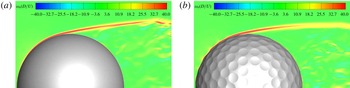
Contours of the instantaneous azimuthal vorticity
 $\unicode[STIX]{x1D714}_{\unicode[STIX]{x1D703}}$
for the (a) smooth sphere and (b) dimpled sphere. Both panels are at
 $Re=10\,000$
corresponding to the subcritical regime.

Drag statistics for smooth and dimpled spheres.

3 Results
3.1 Flow analysis
Figure 3 shows contours of the instantaneous azimuthal vorticity for the computations in the subcritical regime at
 $Re=1.0\times 10^{4}$
. For both the smooth and dimpled spheres, the boundary layer remains laminar and the flow separates near the top. After separation, a shear layer is formed which becomes unstable farther downstream and sheds vortices in the wake. The drag coefficient for both cases is shown in figure 1 and is also listed in table 1. For the smooth sphere, the drag coefficient is
 $C_{D}=0.413$
, which is in close agreement with experimental results in Wieselsberger (Reference Wieselsberger1922). For the dimpled sphere, this value increases slightly to
 $C_{D}=0.417$
. The dimples in this regime do not appear to have a big impact on the flow physics or the drag coefficient. At
 $Re=1.1\times 10^{5}$
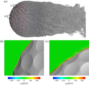
, on the other hand, the dimples trigger transition and the flow enters the post-critical regime. Figure 4(a) shows a visualization of the vortical structures on the dimpled sphere and near wake at one instant in time. An isosurface of the second invariant of the velocity gradient tensor or
 $Q$
-criterion (see Hunt, Wray & Moin Reference Hunt, Wray and Moin1988) is used for this purpose. The surface of the sphere is coloured by the skin friction coefficient. Figure 4(b) and figure 4(c) zoom in over two areas at the front of the sphere and show contours of the azimuthal vorticity,
 $\unicode[STIX]{x1D714}_{\unicode[STIX]{x1D703}}$
. Near the stagnation point, the flow remains attached over the first rows of dimples and the boundary layer is clearly laminar. Further downstream the flow starts to separate locally over the leading edge of the dimple and a detached shear layer is formed.
(a) Flow visualization around the dimpled sphere at an instant in time using an isosurface of
 $Q$
. The surface is coloured by the skin friction coefficient. (b,c) Contours of the instantaneous azimuthal vorticity
 $\unicode[STIX]{x1D714}_{\unicode[STIX]{x1D703}}D/U$
at the areas indicated in panel (a).

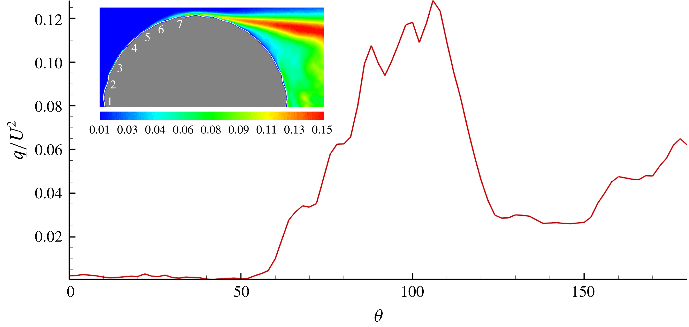
The shear layer becomes unstable and breaks down into smaller vortical structures. This instability is instrumental in the transition of the laminar boundary layer to turbulence, as also pointed out in the experimental study by Choi et al. (Reference Choi, Jeon and Choi2006). The growth of these disturbances and the approximate location of transition to turbulence can be determined by looking at the behaviour of the velocity fluctuations. Figure 5 shows the variation of the turbulent kinetic energy,
 $q$
, averaged over time and in the azimuthal direction, along the surface of the sphere (
 $\unicode[STIX]{x1D703}=0^{\circ }$
at the stagnation point in the front and
 $\unicode[STIX]{x1D703}=180^{\circ }$
at the back). The quantity is plotted along an arc that is located
 $0.05D$
above the surface of the sphere. For reference, the outline of the dimpled sphere along with the dimple count is also shown in the inset. The levels of
 $q$
are negligible at the front part and start to rise after
 $\unicode[STIX]{x1D703}=50^{\circ }$
or approximately the fifth row of dimples. It is therefore reasonable to assume that transition takes places around
 $\unicode[STIX]{x1D703}=50^{\circ }$
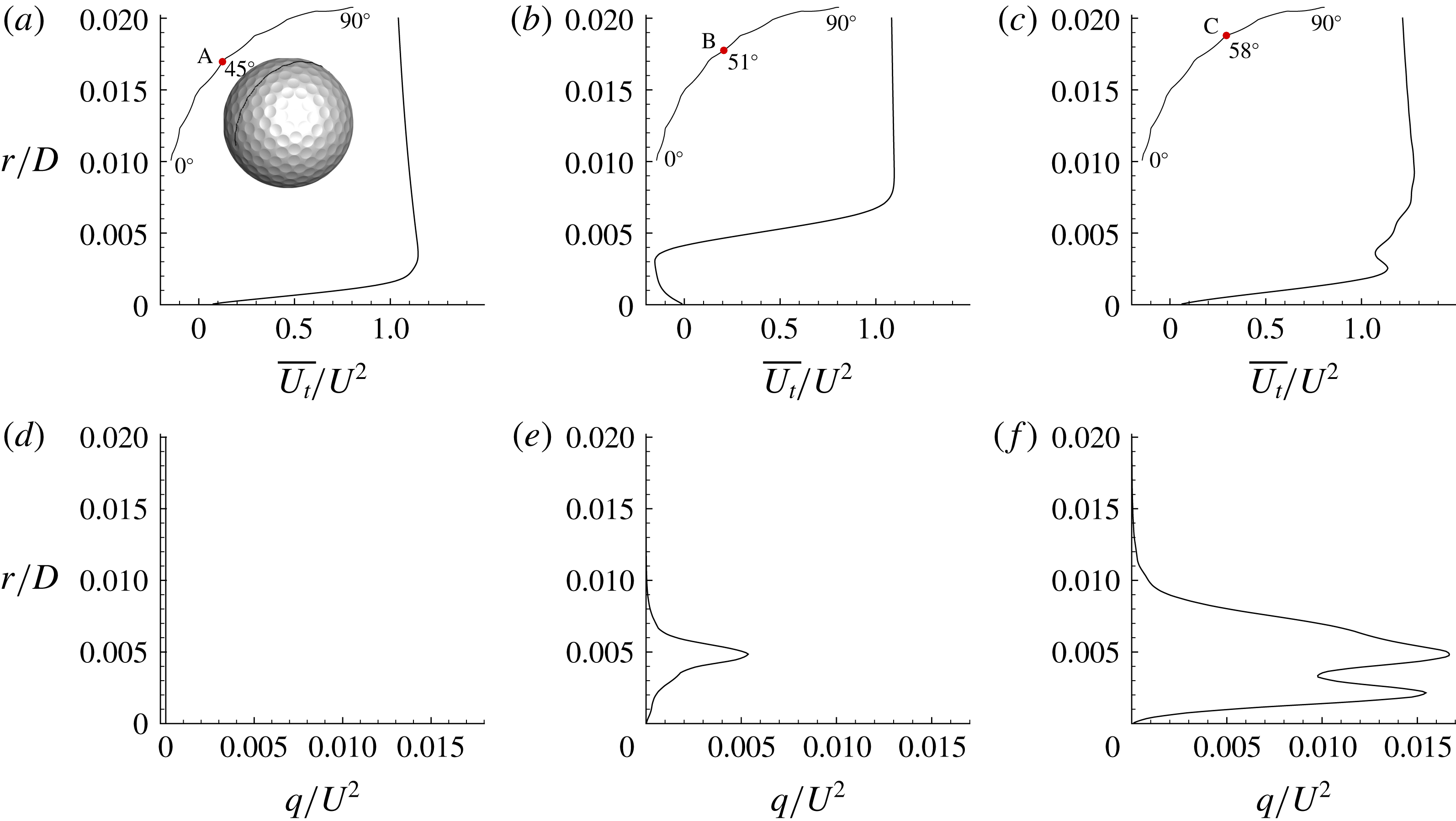
. To further quantify this, profiles of the time-averaged streamwise velocity and turbulent kinetic energy around
 $\unicode[STIX]{x1D703}=50^{\circ }$
are shown in figure 6. Three stations are selected: one before, one inside and one after the fifth row of dimples where transition takes place. At the first station, the velocity profile and the lack of turbulent kinetic energy confirm that the boundary layer is still laminar. Inside the dimple, the velocity profile resembles that of a shear layer and the turbulent kinetic energy has a peak at approximately
 $r/D=0.0045$
. Farther downstream and just after the dimple, the turbulent kinetic energy exhibits two peaks, one at
 $r/D=0.05$
and another closer to the wall at
 $r/D=0.02$
. The first one corresponds to the wake of the shear layer. As we will discuss below, the second peak is a result of streamwise-oriented vortical structures that develop near the wall as a turbulent boundary layer is forming. This result is consistent with the measurements by Choi et al. (Reference Choi, Jeon and Choi2006), where they also reported double peaks in the profiles of the streamwise velocity fluctuations in various locations around the dimple.
Variation of the turbulent kinetic energy,
 $q$
, along an arc at
 $0.05D$
above the surface. The inset (top left) shows contours of
 $q/U^{2}$
. The numerals in the inset indicate the average dimple count from the stagnation point on the front.

(a–c) Profiles of the time-averaged streamwise velocity
 $\overline{U}_{t}$
; (d–f) profiles of the mean turbulent kinetic energy
 $q$
. Statistics are shown at three stations along an azimuthal plane. The locations of the stations are also indicated: A is at
 $\unicode[STIX]{x1D703}=45^{\circ }$
; B is at
 $\unicode[STIX]{x1D703}=51^{\circ }$
; and C is at
 $\unicode[STIX]{x1D703}=58^{\circ }$
.

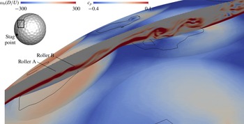
Figure 7 shows contours of the instantaneous azimuthal vorticity at a plane cutting through the middle of a dimple in row 5, where transition occurs (corresponding to the location of the dimple in figure 6). Contours of the instantaneous pressure coefficient,
 $c_{p}$
, are plotted on the surface of the dimpled sphere along with the separation line denoted by the black line. It is clearly seen that a shear layer is formed as the flow separates over the leading edge of the dimple. The flow separation is not uniform across the span and occurs over the first half of the dimple. The flow reattaches again slightly downstream of the dimple centre. It should be noted that, towards the sides, where the dimple depth is smaller, the flow remains attached. Shortly after the flow separates, the shear layer becomes unstable and starts to roll up into vortical structures, annotated as rollers A and B in figure 7. It is important to note that, shortly after the flow reattaches inside the dimples, the pressure increases and reaches a local maximum.
Contours of the instantaneous azimuthal vorticity
 $\unicode[STIX]{x1D714}_{\unicode[STIX]{x1D703}}D/U$
along a plane passing through the middle of a dimple in row 5. The surface is coloured by the instantaneous pressure coefficient
 $c_{p}$
and the black line denotes separation.

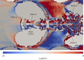
Top view of the vortical structures in the same dimple as shown in figure 7, visualized using an isosurface of
 $Q$
. The structures are coloured by the instantaneous tangential vorticity.

The evolution of these rollers, which is essential in the transition process, can be better traced in figure 8, where a top view of an isosurface of the
 $Q$
-criterion is plotted for the same dimple as shown in figure 7. The vortical structures are coloured by streamwise vorticity. It can be seen that roller A is not uniform in the azimuthal direction and does not extend across the entire span of the dimple: its length in the spanwise direction is approximately one-fifth of the dimple diameter. A similar behaviour can be observed for roller B. As these rollers undergo instabilities in the azimuthal direction, their vorticity is reoriented from the azimuthal to the streamwise direction. Also, in between the two rollers, pairs of counter-rotating streamwise vortices are present. These vortices are reminiscent of the braid vortices containing mainly streamwise vorticity of opposite sign, typically found in free-shear layers undergoing Kelvin–Helmholtz type instability.
Farther downstream and close to the trailing edge of the dimple, a vortical structure resembling a
 $\unicode[STIX]{x039B}$
-type vortex is clearly observed. This
 $\unicode[STIX]{x039B}$
-type vortex has evolved from the continuous bending of a previously shed roller and its legs are connected to a pair of braid vortices. We should note that the rollers aligned primarily in the azimuthal direction are transformed into
 $\unicode[STIX]{x039B}$
-type vortices always within the same dimple for a given Reynolds number. This mechanism is qualitatively identical to the one observed for flow over a dimpled flat plate, where it has been shown that the
 $\unicode[STIX]{x039B}$
vortices quickly evolve into a packet of hairpin-like structures reminiscent of turbulent wall-bounded flows (see Beratlis, Balaras & Squires Reference Beratlis, Balaras and Squires2014). These authors showed that the transition zone is initially confined in a narrow band along the centreline of the dimple, while towards the side there is no activity and the flow remains laminar. The vortical structures originating from this dimple propagate downstream and travel over the subsequent dimple. At the centre of the subsequent dimple, the shear layer does not have a coherent rollup as observed in the previous dimple. Instead a rollup of the shear layer occurs towards the side of the dimple where rollers C and D are highlighted. It is clear that the vortical structures in the second dimple occupy a larger portion of the dimple across the span, and, as the subsequent row of dimples is reached, these structures populate the entire circumference, supporting the growth of a turbulent-like boundary layer.
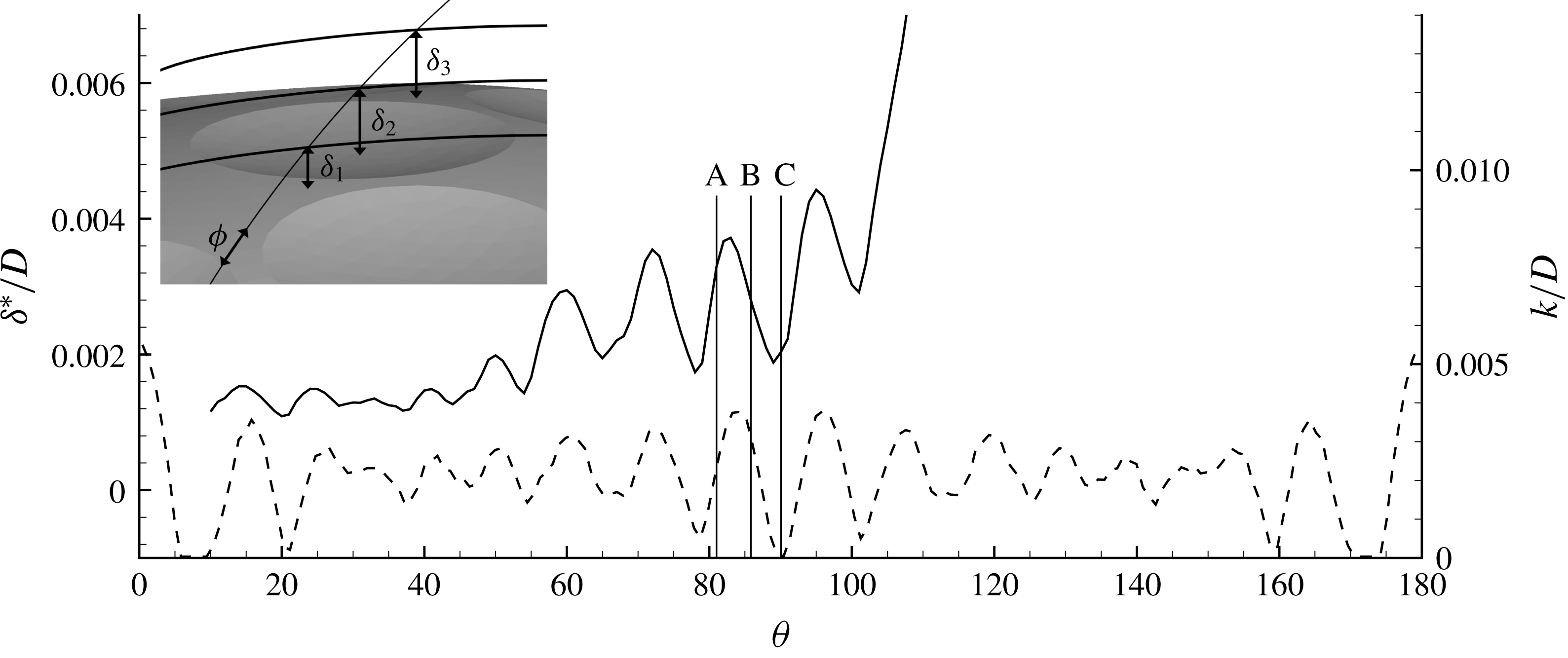
Variation of the space- and time-averaged displacement thickness,
 $\unicode[STIX]{x1D6FF}^{\ast }/D$
, and dimple depth,
 $k/D$
, along the surface of the sphere: ——,
 $\unicode[STIX]{x1D6FF}^{\ast }$
; - - - -,
 $k$
. The vertical lines correspond to the locations shown in figure 10.

To better understand how this boundary layer evolves, figure 9 shows the average boundary layer displacement thickness,
 $\unicode[STIX]{x1D6FF}^{\ast }$
, as a function of the polar angle
 $\unicode[STIX]{x1D703}$
, up to the separation point. Since the location of the wall varies in the azimuthal direction, the displacement thickness is first calculated at each azimuthal plane, as shown in the inset of figure 9. This gives a set of displacement thicknesses
 $\unicode[STIX]{x1D6FF}_{1}^{\ast },~\unicode[STIX]{x1D6FF}_{2}^{\ast },\ldots ,\unicode[STIX]{x1D6FF}_{n}^{\ast }$
with respect to the local wall location, which are then averaged over the azimuthal direction
 $\unicode[STIX]{x1D719}$
to give
 $\unicode[STIX]{x1D6FF}^{\ast }$
. Note that
 $\unicode[STIX]{x1D6FF}^{\ast }$
is calculated utilizing the vorticity definition proposed by Spalart & Watmuff (Reference Spalart and Watmuff1993), which is more appropriate in the presence of curvature and pressure gradients. It is clear that the boundary layer does not grow in a monotonic fashion, as it would for a smooth sphere, and there are local peaks and valleys associated with the presence of the dimples (for reference, the average dimple depth is shown on the lower part of figure 9). The peaks and valleys in
 $\unicode[STIX]{x1D6FF}^{\ast }$
correspond to the location of the maximum and minimum dimple depth, respectively, and, overall, dimples promote a thickening of the boundary layer. Although direct comparisons to classical boundary layer correlations may not be meaningful here, due to the effects of the local pressure gradients, the results are consistent with our earlier work on the evolution of zero-pressure-gradient boundary layers on a flat plate covered with dimples. In particular, we demonstrated that the boundary layer grows at a similar rate as on a smooth plate, but, depending on the type of dimples, there is a distinct shift in the virtual origin of the boundary layer (see Beratlis et al.
Reference Beratlis, Balaras, Squires and Vizard2016, for details). The momentum thickness, although not shown here, behaves in a similar manner.
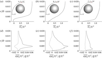
(a–c) Profiles of the mean tangential velocity; (d–f) mean turbulent kinetic energy
 $q/U^{2}$
and Reynolds stresses
 $\overline{u_{t}^{\prime }u_{n}^{\prime }}/U^{2}$
. The statistics are averaged over time and are shown at three stations along an azimuthal plane. The locations of the stations are also indicated: A is at
 $\unicode[STIX]{x1D703}=81^{\circ }$
; B is at
 $\unicode[STIX]{x1D703}=86^{\circ }$
; and C is at
 $\unicode[STIX]{x1D703}=90^{\circ }$
.

Profiles of the tangential velocity
 $\overline{U}_{t}$
, turbulent kinetic energy
 $\overline{q}$
, and the cross Reynolds stresses
 $\overline{u_{t}^{\prime }u_{n}^{\prime }}$
at three stations in the vicinity of a dimple near
 $\unicode[STIX]{x1D703}=90^{\circ }$
are shown in figure 10. Despite the considerable thickening of the boundary layer at this station, the local dimple topology still directly influences the local flow. In the front part of the dimple, the flow separates locally and there is one peak in the turbulent kinetic energy and the Reynolds stresses at
 $r=0.004D$
corresponding to the location of the shear layer (see figure 10
a). Towards the trailing edge of the dimple, the flow reattaches as shown in figure 10(b), and the profile of the turbulent kinetic energy exhibits two peaks, one close to the wall at
 $r=0.0025D$
and another one at
 $r=0.005D$
. The latter is a remnant of the turbulent kinetic energy produced at the shear layer, while the former is an indication of the turbulent activity close to the wall. As one exits the dimple, the velocity profile indicates more momentum near the wall, and the turbulent kinetic energy and Reynolds stresses exhibit only one peak very close to the wall (see figure 10
c). Note that, unlike an equilibrium turbulent boundary layer, the levels of
 $q$
and
 $\overline{u_{t}^{\prime }u_{n}^{\prime }}$
do not decay very quickly as one moves away from the wall. Overall, the turbulent-like boundary layer that forms over the dimpled surface is directly affected by the underlying topology and the local pressure gradients that it induces. Pockets of local separation exist throughout the dimples after transition occurs, until the point of global separation. The details on the local and global separation as well as its impact on the drag force are given in the following section.
3.2 Origin of the drag force
In this section we will compute the contributions to the total drag from the pressure and skin friction and compare it to that of a smooth sphere in the same flow regime. A sphere enters the post-critical regime at a much higher Reynolds number than a dimpled sphere, and performing such a simulation is prohibitively expensive. For that reason, data from the smooth sphere experiments of Achenbach (Reference Achenbach1972) at
 $Re=1.1\times 10^{6}$
are selected for the comparison in the post-critical regime. To our knowledge these are the only experiments on flow over a smooth sphere in the post-critical regime that report pressure and skin friction coefficients.
The drag coefficient is calculated by integrating the pressure and shear stress forces over the surface of the body using the following formula:
 $$\begin{eqnarray}C_{D}=\underbrace{\frac{1}{\unicode[STIX]{x1D70C}U^{2}A_{x}}\int ^{A}p\,\text{d}A_{x}}_{C_{Dp}}+\underbrace{\frac{1}{\unicode[STIX]{x1D70C}U^{2}A_{x}}\int ^{A}(\unicode[STIX]{x1D70F}_{xx}+\unicode[STIX]{x1D70F}_{xz}+\unicode[STIX]{x1D70F}_{xz})\,\text{d}A_{x}}_{C_{Df}},\end{eqnarray}$$
where
 $A_{x}$
denotes the frontal area of the sphere,
 $p$
is the pressure,
 $\unicode[STIX]{x1D70F}_{xx}$
,
 $\unicode[STIX]{x1D70F}_{xz}$
and
 $\unicode[STIX]{x1D70F}_{xz}$
are the components of the shear stress tensor, and
 $\unicode[STIX]{x1D70C}$
and
 $U$
are the density of the fluid and the free-stream velocity, respectively. The terms on the right-hand side,
 $C_{Dp}$
and
 $C_{Df}$
, represent the contributions to the total drag from the pressure and the skin friction, respectively. The skin friction reported below was calculated as
 $C_{f}=(2\unicode[STIX]{x1D708}/U^{2})\,\text{d}U_{t}/\text{d}n$
, where
 $U_{t}$
is the tangential velocity component and
 $n$
is the surface normal.
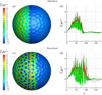
(a,c) Contours of the average skin friction coefficient,
 $\overline{C}_{f}Re^{0.5}$
, on the surface of the dimpled sphere (separation line is shown in solid black) for (a) subcritical (
 $Re=10\,000$
) and (c) post-critical regimes. (b,d) Evolution of the average skin friction coefficient,
 $\overline{C}_{f}Re^{0.5}$
, versus the polar angle,
 $\unicode[STIX]{x1D703}$
, for every point on the sphere for (b) subcritical (
 $Re=10\,000$
) and (d) post-critical regimes. Lines and symbols represent: red ●, dimpled sphere, land area, present DNS; green ●, dimpled sphere, dimpled area, present DNS; ——, smooth sphere at
 $Re=10\,000$
and
 $Re=1.14\times 10^{6}$
, Achenbach (Reference Achenbach1972).

Figure 11 shows contours of the time-averaged skin friction coefficient,
 $\overline{C}_{f}$
, on the surface of the dimpled sphere, along with the separation line indicated by the solid black line for both flow regimes. For the subcritical regime, the flow remains attached at the front part of the sphere and there is no local separation inside the dimples. The highest values of
 $C_{f}$
are observed around
 $\unicode[STIX]{x1D703}=45^{\circ }$
and occur just downstream of the dimple’s trailing edge. Global separation occurs near the top of the sphere and appears to be influenced by the presence of the dimples. In the presence of a dimple, the flow separates at its leading edge, while between dimples the separation is slightly delayed. As a result the separation line is non-uniform in the azimuthal direction. A more quantitative analysis of the skin friction is shown in figure 11(b), where the
 $\overline{C}_{f}$
is plotted separately on the dimpled and land (non-dimpled) areas.
For reference,
 $C_{f}$
for a smooth sphere at the same Reynolds numbers is superimposed. For the most part
 $\overline{C}_{f}$
is higher than that of a sphere on the land area and smaller inside the dimples. The peak values of
 $\overline{C}_{f}$
are approximately twice as high as that of a smooth sphere at the front part.
For the post-critical regime, the behaviour of
 $\overline{C}_{f}$
is very different. As shown in figure 11(d), the flow starts to separate locally inside the dimples as early as
 $\unicode[STIX]{x1D703}=45^{\circ }$
and continues to separate within each dimple after that. The local separation is consistent with the formation of shear layers and the onset of transition triggered by the dimples. Figure 11(d) plots
 $\overline{C}_{f}$
versus the polar angle
 $\unicode[STIX]{x1D703}$
on every point on the sphere. For reference the average skin friction for a smooth sphere at a post-critical Reynolds number,
 $Re_{D}=1.14\times 10^{6}$
, measured by Achenbach (Reference Achenbach1972) is also plotted. Note that
 $\overline{C}_{f}$
is scaled by
 $Re^{0.5}$
in order to account for the difference in Reynolds numbers between the two spheres. This scaling was originally used by Achenbach (Reference Achenbach1972) to plot
 $C_{f}$
for a wide range of Reynolds numbers and the correlation was very good. Again the peaks in
 $\overline{C}_{f}$
which occur both near the trailing edge of the dimples and on the land area are higher than the
 $C_{f}$
for a smooth sphere at the corresponding polar angle by as much as a factor of two. The highest value of
 $\overline{C}_{f}$
for the dimpled sphere occurs around
 $\unicode[STIX]{x1D703}=80^{\circ }$
. The flow eventually separates at the back of the sphere (global separation) and the separation line varies significantly in the azimuthal direction depending on the dimple arrangement. Figure 11(d) reveals that global separation can occur as late as 120
 $^{\circ }$
at some azimuthal locations, which is similar to the case of a smooth sphere in the post-critical regime.
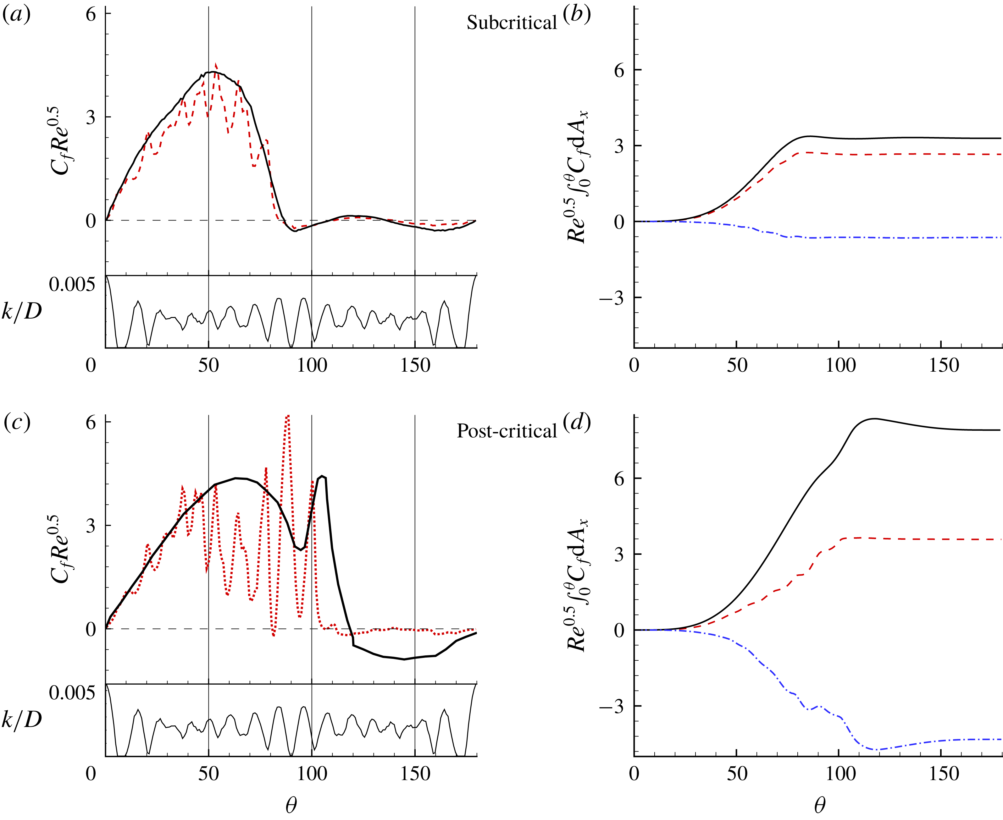
The contribution of
 $C_{f}$
to the total drag is assessed next. The upper part of figure 12(a) shows the skin friction coefficient,
 $C_{f}$
, averaged over time and azimuthal direction for the subcritical regime. The average dimple depth distribution
 $k/D$
is also plotted in the lower part of figure 12(a). It is evident that
 $C_{f}$
is inversely correlated with the average dimple depth. In particular, the local minima in
 $C_{f}$
correspond to local maxima in
 $k/D$
and vice versa. As the flow enters the dimple, the local deceleration causes
 $C_{f}$
to decrease and then, as the flow approaches the trailing edge of the dimple, it accelerates, causing an increase in
 $C_{f}$
. Overall, the average
 $C_{f}$
for the dimpled sphere is consistently lower than that of a smooth sphere at the front part. Global separation, identified as the crossing from positive to negative values of
 $C_{f}$
, occurs at
 $\unicode[STIX]{x1D703}=87^{\circ }$
and
 $\unicode[STIX]{x1D703}=85^{\circ }$
for the smooth and dimpled spheres, respectively. The integral of the skin friction (scaled by
 $Re^{0.5}$
) as a function of
 $\unicode[STIX]{x1D703}$
is shown in figure 12(b). When the integral is evaluated over the entire sphere, it is equal to the skin friction drag. For the smooth sphere, the skin friction drag is 0.035, or 8.5 % of the total drag, while for the dimpled sphere, the skin friction is slightly lower, 0.030, or approximately 7.2 % of the total drag.
For the post-critical regime, the mean
 $C_{f}$
is shown in figure 12(c). For the dimpled sphere,
 $C_{f}$
is considerably lower than that of a smooth sphere from
 $\unicode[STIX]{x1D703}=45^{\circ }$
to
 $\unicode[STIX]{x1D703}=90^{\circ }$
. This is the region downstream of the transition point where the local flow separation occurs inside the dimples. As a result, when looking at the integral of
 $C_{f}$
plotted in figure 12(d), the overall skin friction drag for the dimpled sphere is approximately half of that for a smooth sphere. The above analysis establishes an interesting point, that dimples actually contribute less friction drag than a smooth sphere. The skin friction drag decrease is very small in the subcritical regime but it becomes more important in the post-critical regime due to local flow separation patterns inside the dimples. This is in contrast to the commonly accepted view that dimples substantially increase the skin friction drag. Overall the skin friction drag accounts for less than 10 % of the total drag. Finally, as shown in figure 12(d), global separation for the dimpled sphere occurs on average around
 $\unicode[STIX]{x1D703}=112^{\circ }$
while for a smooth sphere it occurs around
 $\unicode[STIX]{x1D703}=119^{\circ }$
.
(a,c) Skin friction coefficient
 $C_{f}$
(upper part) and dimple depth
 $k$
(lower part) versus polar angle
 $\unicode[STIX]{x1D703}$
in (a) the subcritical regime (
 $Re=10\,000$
) and (c) the post-critical regime. Both quantities are averaged over time and azimuthal direction. (b,d) Cumulative integral of the friction drag in (b) the subcritical regime (
 $Re=10\,000$
) and (d) the post-critical regime. Lines represent: - - - -, dimpled sphere; ——, smooth sphere; and — ⋅ —, difference between dimpled and smooth spheres.

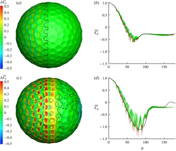
(a,c) Contours of the difference
 $\unicode[STIX]{x0394}\overline{C}_{p}$
between the average pressure coefficient
 $\overline{C}_{p}$
of the dimpled and smooth spheres plotted on the surface of the dimpled sphere (separation line,
 $\overline{C}_{f}=0$
, is shown in solid black) for (a) subcritical (
 $Re=10\,000$
) and (c) post-critical regimes. (b,d) Evolution of the average,
 $\overline{C}_{p}$
, versus the polar angle,
 $\unicode[STIX]{x1D703}$
, for every point on the sphere for (b) subcritical (
 $Re=10\,000$
) and (d) post-critical regimes. Lines and symbols represent: red ●, dimpled sphere, land area, present DNS; green ●, dimpled sphere, dimpled area, present DNS; black ——, smooth sphere at
 $Re=1.14\times 10^{6}$
, Achenbach (Reference Achenbach1972).

Pressure, which is the other component that contributes to drag, is analysed next. Figure 13(a) shows contours of the time-averaged pressure ‘penalty’ coefficient,
 $\unicode[STIX]{x0394}\overline{C}_{p}$
. This is the difference in
 $\overline{C}_{p}$
between the dimpled and smooth spheres. Figure 13(b) also plots the time-averaged
 $\overline{C}_{p}$
on every point on the dimpled sphere. A point inside a dimple is shown in green while a point outside a dimple is shown in red. For reference,
 $\overline{C}_{p}$
for a smooth sphere at the same Reynolds numbers is superimposed. Differences in
 $\overline{C}_{p}$
between the two spheres are observed at the front part. Mainly the pressure inside the dimples appears to be higher than that of a smooth sphere, while outside the dimples the reverse holds true. However, these differences are very small in the subcritical regime. In the post-critical regime, the pressure ‘penalties’ are significantly amplified. Figure 13(c), which shows the contours of
 $\unicode[STIX]{x0394}\overline{C}_{p}$
along with the separation line indicated by a black line, reveals that when local separation inside the dimples starts occurring around
 $\unicode[STIX]{x1D703}=45^{\circ }$
, the levels of
 $\overline{C}_{p}$
rise. The
 $\unicode[STIX]{x0394}\overline{C}_{p}$
value appears to be positive downstream of the reattachment line and towards the trailing edge of the dimple. Figure 13(d) also shows that, as the angle
 $\unicode[STIX]{x1D703}$
increases from
 $45^{\circ }$
, the peak values in
 $\overline{C}_{p}$
become larger with respect to that of a smooth sphere.
(a,c) Variation of
 $C_{p}$
(upper part) and dimple depth
 $k$
(lower part) averaged over time and azimuthal direction versus polar angle
 $\unicode[STIX]{x1D703}$
in (a) the subcritical regime (
 $Re=10\,000$
) and (c) the post-critical regime. The vertical dashed line corresponds to a local peak in
 $C_{p}$
. (b,d) Cumulative integral of the pressure drag in (b) the subcritical regime (
 $Re=10\,000$
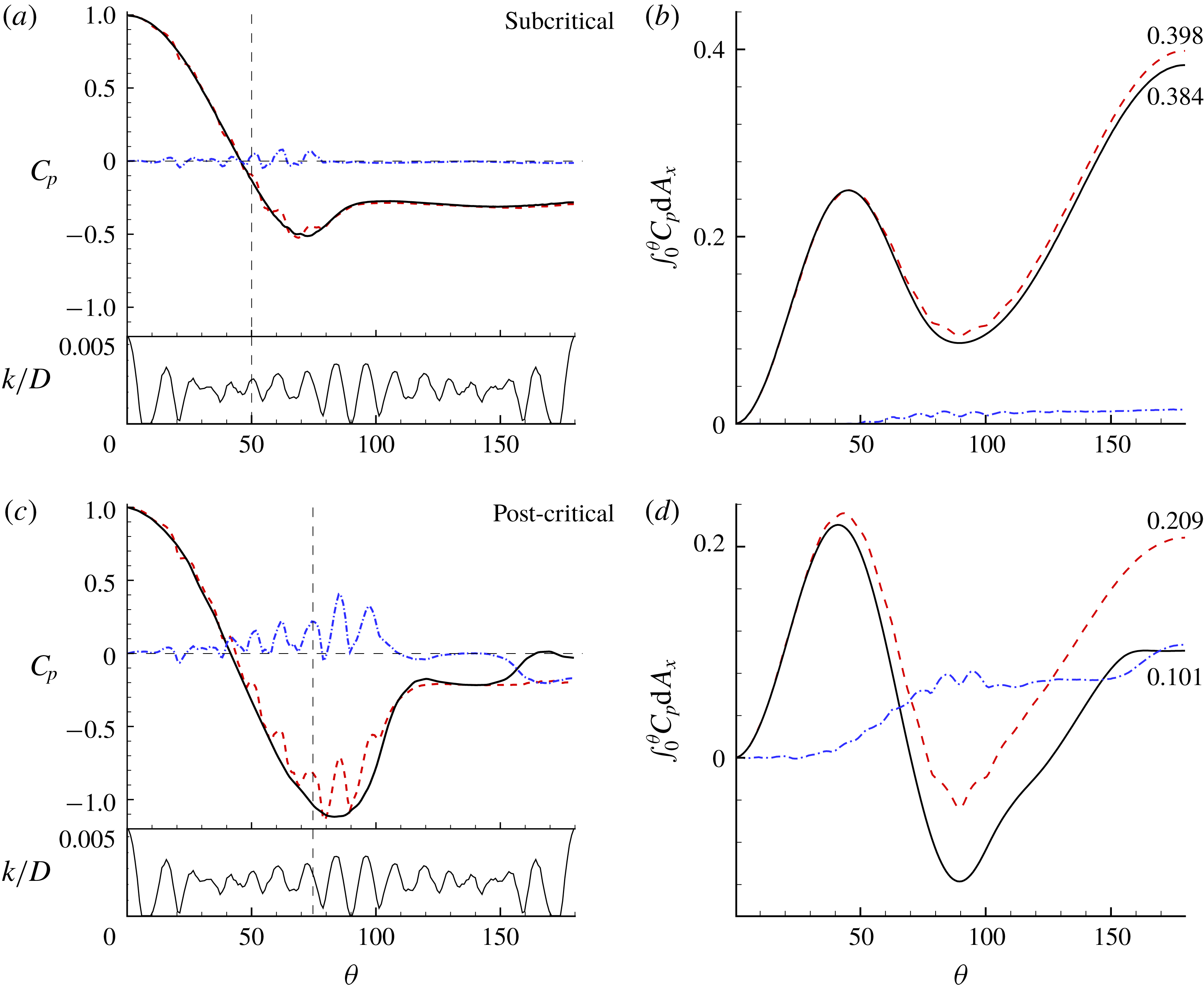
) and (d) the post-critical regime. Lines represent: - - - -, dimpled sphere; ——, smooth sphere; — ⋅ —, difference between dimpled and smooth spheres.

A more quantitative analysis of the pressure as well as its contribution to the total drag is shown in figure 14. The mean pressure coefficient
 $C_{p}$
for both spheres in the subcritical regime along with the mean dimple depth are shown in figure 14(a). For the dimpled sphere,
 $C_{p}$
exhibits small oscillations forming peaks and valleys. The average depth distribution
 $k/D$
indicates that at the front part of the sphere
 $C_{p}$
is correlated with the average dimple depth. In particular, the local peak in
 $C_{p}$
corresponds to local maxima in
 $k/D$
and vice versa. Overall, the
 $C_{p}$
distributions for both spheres are in close agreement with each other, and the pressures at the back of the spheres are identical. This is expected, as global separation is practically unchanged. The integral of the pressure coefficient as a function of
 $\unicode[STIX]{x1D703}$
is shown in figure 14(b). When the integral is evaluated over the entire sphere, it is equal to the total pressure drag. It is observed that, from the stagnation point up to
 $\unicode[STIX]{x1D703}=50^{\circ }$
, dimples do not incur any pressure penalty, as the local peaks and valleys cancel each other out. After
 $\unicode[STIX]{x1D703}=50^{\circ }$
and up to the global separation point, dimples contribute only a small amount to the pressure drag. The total pressure drag is 0.384 and 0.398 for the smooth and dimpled spheres, respectively.
Figure 14(c) plots
 $C_{p}$
averaged over time and azimuthal direction for the post-critical regime. The plot of the average dimple depth is also shown in the lower part. The fluctuations of
 $C_{p}$
are clearly observed in this regime too. Up to
 $\unicode[STIX]{x1D703}=45^{\circ }$
, that is, before the boundary layer transitions, the fluctuations are relatively small and
 $C_{p}$
appears to oscillate around
 $C_{p}$
of a smooth sphere, as is evident by the blue dash-dotted line representing the difference in
 $C_{p}$
between the two spheres. However, after
 $\unicode[STIX]{x1D703}=45^{\circ }$
, the fluctuations in
 $C_{p}$
increase in magnitude, and
 $C_{p}$
for the dimpled sphere is consistently higher than that of a smooth sphere. The highest fluctuation takes place around
 $\unicode[STIX]{x1D703}=90^{\circ }$
. The locations of the peaks in
 $C_{p}$
correspond to shortly after the location of the maximum dimple depth. This is approximately downstream of where the flow reattaches inside the dimple. Overall, the pressure on the dimpled sphere is higher on the front part from the transition point and up to the global separation line around
 $\unicode[STIX]{x1D703}=120^{\circ }$
. This indicates that dimples incur a local pressure penalty compared to a smooth sphere. After global separation, the base pressure at the back of the sphere does not exhibit any fluctuations and remains flat and in close agreement with that of a smooth sphere.
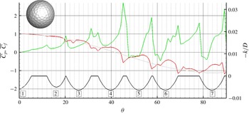
To better understand the link between the pressure and the flow topology inside the dimples, figure 15 plots the time-averaged pressure and skin friction coefficients along a line cutting through the golf ball. The plot focuses on the front part of the sphere. The variation of the dimple depth and the dimple number are shown at the bottom, while the pressure coefficient for a smooth sphere is overlayed for reference. The pressure does not behave in a monotonic fashion like that for a smooth sphere. Although it decreases from the stagnation point, it does so forming local peaks and valleys. During the first four dimples, the boundary layer is attached as
 $\overline{C}_{f}$
remains positive. The flow remains laminar and the difference between the local pressure maxima and minima is relatively small. The first local flow separation inside a dimple occurs at the fifth dimple at approximately
 $\unicode[STIX]{x1D703}=45^{\circ }$
as the skin friction coefficient crosses from positive to negative values. In general, as the flow decelerates towards the leading edge of the dimple, the pressure coefficient starts to rise. Local maxima in the pressure occur shortly after the flow reattaches inside the dimple. At the trailing edge of the dimple, as the flow accelerates, the skin friction coefficient reaches a local maximum while the pressure reaches a local minimum.
Variation of the time-averaged pressure and skin friction coefficient along a line cutting through the front part of the dimpled sphere. The variation of the surface is shown at the bottom with numerals indicating the dimple count. Lines represent: red ——,
 $\overline{C}_{p}$
, dimpled sphere; grey ——,
 $\overline{C}_{p}$
, smooth sphere at
 $Re=1.14\times 10^{6}$
, Achenbach (Reference Achenbach1972); green ——,
 $\overline{C}_{f}$
, dimpled sphere; black ——,
 $-k/D$
, dimpled sphere.

The integral of the pressure over the surface area for the dimpled and smooth spheres in the post-critical regime is shown in figure 14(d). The integral is plotted versus
 $\unicode[STIX]{x1D703}$
, and when evaluated over the entire surface (
 $\unicode[STIX]{x1D703}=0{-}180^{\circ }$
) it gives the total drag coefficient due to pressure. The difference in the integrals between the dimpled and smooth spheres is also shown and helps identify the source of the drag penalty. Initially the pressure integrals up to
 $\unicode[STIX]{x1D703}=45^{\circ }$
are equal, revealing that the first few dimples do not impose any significant pressure penalty. The main drag penalty comes from the dimples located between
 $45^{\circ }<\unicode[STIX]{x1D703}<90^{\circ }$
. In that region the pressure drag overhead due to the dimples becomes very important and already at
 $\unicode[STIX]{x1D703}=90^{\circ }$
this penalty is approximately
 $0.08$
, which is approximately 50 % of the total drag force on the smooth sphere. It is also an order of magnitude higher than the penalty due to skin friction. An additional pressure penalty of
 $0.03$
occurs due to differences in the base pressure at the back of the body. A summary of the relative contributions of the pressure and friction drag to the total as well as the differences for the smooth and dimpled sphere are given in table 1.
4 Conclusions
Dimples reduce the value of the critical Reynolds number, which marks the regime where the boundary layers on the surface of the sphere become turbulent-like. This also results in a drastic reduction of the drag coefficient when compared to that of the smooth sphere at the same Reynolds number. The main mechanism behind the significant reduction is the global separation delay due to the fact that the flow is now energized near the wall and carries more momentum compared to a laminar boundary layer. However, in the post-critical regime, the minimum drag coefficient on a dimpled sphere is significantly higher (approximately 2.5 times) than the minimum drag coefficient of a smooth sphere. The source of this difference, which is not explained by existing experimental results, has been the focus of the present work.
We report DNS of the flow around dimpled spheres in the subcritical and post-critical regimes. The former reveals that dimples do not impose any significant pressure or viscous penalties and the drag remains practically unchanged when compared to a smooth sphere. In the post-critical regime, however, we report two important features: (i) dimples decrease the mean skin friction coefficient, which rectifies the common assumption that dimples typically increase; and (ii) dimples, despite their small size, incur a local pressure penalty, which is significant and accounts for most of the difference in drag between a smooth and a dimpled sphere in the post-critical regime.
Detailed analysis showed that the dimples at the frontal area of the sphere do not contribute significantly to the pressure overhead. The pressure penalties become important right after transition occurs, which for this particular geometry and Reynolds number comes at
 $45^{\circ }$
. As the flow separates over the dimples, the skin friction decreases and the pressure increases. The maximum in the pressure occurs shortly downstream of the flow reattachment. After the reattachment, the skin friction starts to increase and the pressure decreases. When compared to a smooth sphere in the post-critical regime, the pressure inside the largest portion of the dimple is higher at the same polar angle
 $\unicode[STIX]{x1D703}$
. Overall, the pressure penalty imposed by dimples at the front of the sphere, from
 $\unicode[STIX]{x1D703}=45^{\circ }$
to
 $\unicode[STIX]{x1D703}=90^{\circ }$
, is approximately 50 % of the total drag force on the smooth sphere.
Overall, the present work puts into perspective the role of the dimples in the drag reduction process. Clearly their geometry and arrangement control the critical Reynolds number, as well as the minimum drag coefficient that can be achieved in the post-critical regime. Our results contribute to the understanding of the underlying flow physics that controls these processes. How to translate these findings into optimal dimple designs, however, is a complex problem that cannot be addressed within the framework of the present work. The primary reason is that we only report results on one dimple geometry (characteristic of a commercial golf ball) at two Reynolds numbers. Preliminary computations (not reported in the present paper) on a geometry with fewer dimples of the same size as the one considered here, as well as the experiments by Aoki and co-workers reported above, indicate that reducing the minimum drag coefficient in the post-critical regime tends to shift the drag crisis towards higher Reynolds numbers, which also significantly affects performance in the case of a golf ball. To accurately map this behaviour requires a full parametric scan of dimple shape, size, depth and arrangement, which is prohibitive in terms of the computational cost. Ongoing work combines synergetic experiments and computations that scan a much wider parametric regime in a cost-efficient manner, which will be the topic of a future paper.