





1. Introduction
Magnetoconvection (MC) is prevalent in astrophysics, geophysics and various engineering applications (Davidson Reference Davidson1999; Jones Reference Jones2011; Weiss & Proctor Reference Weiss and Proctor2014; Davidson Reference Davidson2017). Examples include the dynamo effect in the Earth's inner core (Aurnou & King Reference Aurnou and King2017; Moffatt & Dormy Reference Moffatt and Dormy2019), crystal growth in electromagnetic metallurgy (Moreau Reference Moreau1999) and cooling systems in nuclear fusion reactors (Barleon, Casal & Lenhart Reference Barleon, Casal and Lenhart1991; Ihli et al. Reference Ihli, Basu, Giancarli, Konishi, Malang, Najmabadi, Nishio, Raffray, Rao and Sagara2008). A typical paradigm of buoyancy-driven convection is Rayleigh–Bénard convection (RBC), extensively studied through experiments and numerical simulations (Ahlers, Grossmann & Lohse Reference Ahlers, Grossmann and Lohse2009; Lohse & Xia Reference Lohse and Xia2010; Chillà & Schumacher Reference Chillà and Schumacher2012; Ecke & Shishkina Reference Ecke and Shishkina2023).
The RBC system can be briefly described as due to the heating of the lower part and the cooling of the upper part, a temperature gradient generates inside the fluid layer driving the fluid to form self-organized movement. For such a canonical RBC system, the controlling non-dimensional parameters are the Rayleigh number  $Ra$, the Prandtl number
 $Pr$ and the aspect ratio
 $\varGamma$. The Rayleigh number is the ratio of buoyancy to viscous force representing the ability of thermal driving. The Prandtl number exhibits the inherent physical properties of the working fluid. The effect of geometric confinement on the flow is reflected in the aspect ratio. The non-dimensional parameters mentioned above are defined as
 $Ra=\alpha g \Delta T H^3/\nu \kappa$,
 $Pr=\nu /\kappa$,
 $\varGamma =D/H$, where
 $g$ is the gravitational acceleration,
 $\Delta T=T_b-T_t$ is the temperature difference between the upper and lower plates,
 $H$ is the distance between the plates and
 $D$ is the width of the cell. The physical properties
 $\alpha$,
 $\nu$,
 $\kappa$ and
 $\rho$ represent the thermal expansion coefficient, kinematic viscosity, thermal diffusivity and density of the fluid, respectively.
In the context of MC systems, an additional non-dimensional parameter known as the Hartmann number  $Ha$ is introduced, defined as
 $Ha=BH\sqrt {{\sigma }/{\rho \nu }}=Q^{1/2}$, quantifying the strength of the external magnetic field, where
 $B$ is the strength of the applied external magnetic field and
 $\sigma$ is the electrical conductivity,
 $Q$ is the Chandrasekhar number (Chandrasekhar Reference Chandrasekhar1961). It is worth mentioning that, to ensure consistency in characteristic length throughout the study, we also use
 $H$ as the characteristic length when calculating the
 $Ha$ number. In the MC system the effect of advection of
 $B$ by the flow relative to magnetic diffusion, quantified by the magnetic Reynolds number
 $Rm$, is crucial. In the present experiment,
 $Rm \leqslant 8.31 \times 10^{-3}$ is typically quite small, making the induced magnetic field negligible compared with the applied magnetic field (Davidson Reference Davidson2017).
In the MC or RBC system, two key response parameters are the Nusselt number  $Nu$ and the Reynolds number
 $Re$, defined as
 $Nu=qH/(\lambda \Delta T)$,
 $Re=Ul/\nu$, where
 $q$ represents the heat flux applied to the system,
 $\lambda$ is the thermal conductivity,
 $U$ denotes the typical velocity and
 $l$ stands for the characteristic length. These response parameters serve to quantify the heat transport efficiency and momentum transport efficiency.
In the MC system, beyond the buoyancy force induced by the temperature gradient, the flow dynamics is also influenced by the Lorentz force generated by the applied magnetic field (Davidson Reference Davidson2017). The orientation of the static magnetic field significantly affects the flow dynamics. When the magnetic field aligns vertically, parallel to gravity, convection tends to be suppressed due to Joule dissipation, which leads to a significant reduction in momentum perpendicular to the external magnetic field. Additionally, the magnetic field can inhibit the onset of convection. The critical value of  $Ra$ for convection onset has been extensively studied through linear analysis (Chandrasekhar Reference Chandrasekhar1961; Cioni, Chaumat & Sommeria Reference Cioni, Chaumat and Sommeria2000; Houchens, Witkowski & Walker Reference Houchens, Witkowski and Walker2002), with an asymptotic solution derived by Busse (Reference Busse2008). The stabilizing effect of the vertical magnetic field enhances the coherence of flow structures (Lim et al. Reference Lim, Chong, Ding and Xia2019; Yan et al. Reference Yan, Calkins, Maffei, Julien, Tobias and Marti2019), leading to the emergence of multiple flow structures (Zürner et al. Reference Zürner, Schindler, Vogt, Eckert and Schumacher2020). One of the most intriguing findings under the influence of a vertical magnetic field, observed in numerical simulations (Liu, Krasnov & Schumacher Reference Liu, Krasnov and Schumacher2018; Akhmedagaev et al. Reference Akhmedagaev, Zikanov, Krasnov and Schumacher2020) and experiments (Zürner et al. Reference Zürner, Schindler, Vogt, Eckert and Schumacher2020; Grannan et al. Reference Grannan, Cheng, Aggarwal, Hawkins, Xu, Horn, Sánchez-Álvarez and Aurnou2022), is the widely recognized flow regime known as the wall mode, characterized by significantly high velocity magnitudes near the side walls.
For the horizontal magnetic field perpendicular to gravity, the flow adopts a quasi-two-dimensional (Q2-D) structure characterized by several elongated rolls aligned along the magnetic field direction (Fauve, Laroche & Libchaber Reference Fauve, Laroche and Libchaber1981; Burr & Müller Reference Burr and Müller2002; Yanagisawa et al. Reference Yanagisawa, Hamano, Miyagoshi, Yamagishi, Tasaka and Takeda2013; Vogt et al. Reference Vogt, Ishimi, Yanagisawa, Tasaka, Sakuraba and Eckert2018; Yang, Vogt & Eckert Reference Yang, Vogt and Eckert2021; Chen, Wang & Ni Reference Chen, Wang and Ni2024a). It is worth noting that in their works where convection cells exhibit large  $\varGamma$, geometrical confinement effects on the flow tend to make the convection roll appear quasi-two dimensional and be arranged side by side along the width direction. The introduction of a horizontal magnetic field can induce diverse flow dynamics. Transition between different numbers of Q2-D rolls with spontaneous flow reversal is observed (Yanagisawa et al. Reference Yanagisawa, Yamagishi, Hamano, Tasaka and Takeda2011; Chen et al. Reference Chen, Wang and Ni2024a), with the number of rolls depending on the ratio of
 $Ra/Q$ (Yanagisawa et al. Reference Yanagisawa, Yamagishi, Hamano, Tasaka and Takeda2011, Reference Yanagisawa, Hamano, Miyagoshi, Yamagishi, Tasaka and Takeda2013). As the imbalance between buoyancy and Lorentz force increases, three-dimensional (3-D) oscillation of the flow structure emerges, accompanied by secondary flows resulting from Ekman pumping (Vogt et al. Reference Vogt, Ishimi, Yanagisawa, Tasaka, Sakuraba and Eckert2018). Most experiments or numerical simulations have been conducted in large aspect ratio cells (
 $\varGamma > 1$), where the geometrical confinement effect in the width direction of the cell is less pronounced. At the same time, a significant amount of work is focused on the cylindrical cell, which benefits from its perfect symmetry (Takeshita et al. Reference Takeshita, Segawa, Glazier and Sano1996; Cioni, Ciliberto & Sommeria Reference Cioni, Ciliberto and Sommeria1997; King & Aurnou Reference King and Aurnou2013; Scheel & Schumacher Reference Scheel and Schumacher2016; Zürner et al. Reference Zürner, Schindler, Vogt, Eckert and Schumacher2020; Ren et al. Reference Ren, Tao, Zhang, Ni, Xia and Xie2022; Schindler et al. Reference Schindler, Eckert, Zürner, Schumacher and Vogt2022). However, in most applications, the shape of the convection cell is more like a cuboid, and choosing a cuboid cell is more helpful to fit the actual application. Moreover, for cells with small aspect ratios, the flow is constrained in the lateral direction, which has a significant impact on the flow (Zwirner, Tilgner & Shishkina Reference Zwirner, Tilgner and Shishkina2020). In addition, the cuboid cell will also affect the internal flow structures (Chen et al. Reference Chen, Xie, Yang and Ni2023; Chen, Yang & Ni Reference Chen, Yang and Ni2024b). Consequently, a comprehensive understanding of flow behaviours within cuboid cells with
 $\varGamma < 1$ under the influence of horizontal magnetic fields remains underexplored, motivating our current research efforts.
In the case of either RBC or MC, the global transports, including the heat and momentum transport, are crucial to measure the efficiency of such systems. In RBC systems the global transport efficiency of liquid metal has been widely reported (Takeshita et al. Reference Takeshita, Segawa, Glazier and Sano1996; Cioni et al. Reference Cioni, Ciliberto and Sommeria1997; King & Aurnou Reference King and Aurnou2013; Scheel & Schumacher Reference Scheel and Schumacher2016; Ren et al. Reference Ren, Tao, Zhang, Ni, Xia and Xie2022; Schindler et al. Reference Schindler, Eckert, Zürner, Schumacher and Vogt2022; Chen et al. Reference Chen, Yang and Ni2024b). Furthermore, there is also a unified theory corresponding to liquids with extremely small  $Pr$, i.e.
 $Nu\sim Ra^{1/4}$ and
 $Re\sim Ra^{1/2}$ (Grossmann & Lohse Reference Grossmann and Lohse2000; Stevens et al. Reference Stevens, van der Poel, Grossmann and Lohse2013). Unlike the RBC, the moving electrical conductive fluid with the presence of the external magnetic field will induce Joule dissipation, consequently amplifying kinetic and thermal dissipation. This, in turn, diminishes momentum and heat transport efficiency. The global transport efficiencies under the effect of vertical magnetic fields are also investigated. For example, Burr & Müller (Reference Burr and Müller2001) suggested
 $Nu\sim (RaQ)^{2/3}$ for
 $Q \rightarrow \infty$. Bader & Zhu (Reference Bader and Zhu2023) reported scalings
 $Nu-1\sim RaQ^{-1}$ and
 $Re\sim RaPr^{-1}Q^{-5/6}$. Yan et al. (Reference Yan, Calkins, Maffei, Julien, Tobias and Marti2019) have found
 $Re\sim Ra/(PrQ^{2/3})$ for momentum transport derived through balance of forces. In the experimental results of Zürner et al. (Reference Zürner, Schindler, Vogt, Eckert and Schumacher2020), extensive data fitting was employed to derive the relationships for heat and momentum transport, i.e.
 $Nu \sim [1+(5.9\pm 0.3)(Ha/Ha_c)^{(2.03\pm 0.06)}]^{-1}$ and
 $Re \sim [1+(0.68\pm 0.04)N_{ff}^{(0.87\pm 0.03)}]^{-1}$, respectively. Moreover, the extended Grossmann–Lohse theory under the effect of a vertical magnetic field is investigated by Zürner et al. (Reference Zürner, Liu, Krasnov and Schumacher2016). However, few studies have explored the scalings of global transport efficiency under the action of a horizontal magnetic field, which is the main motivation for conducting this experiment.
This study aims to systematically explore the interplay between flow regimes and global transport properties within a broad range of parameters, in the presence of a horizontal magnetic field. An essential contribution of the present paper is the extension of the existing regime diagram towards larger Hartmann numbers up to  $Ha=2041$. In this work, we reconstruct the flow structures by combining the data obtained from temperature and velocity measurements and explore the characteristics of different flow regimes, trying to find unified laws. Additionally, we performed fitting based on a large amount of data and obtained unified scaling laws for heat transport and momentum transport, respectively. We have made great efforts in liquid metal velocity measurement and hope to expand our knowledge in this aspect.
The outline of this paper is organized as follows. In § 2 we provide a brief introduction to our experimental set-up and the methods employed in this study. Flow morphologies and their corresponding regimes are outlined in § 3. Section 4 delves into the investigation of flow characteristics. Section 5 reviews the global transport of heat and momentum. A summary of the work is given in § 6.
2. Experimental set-up and measurement methods
The experiment was carried out in a  $\varGamma \approx 0.5$ (a cuboid cell with height
 $H = 10.2$ cm and width
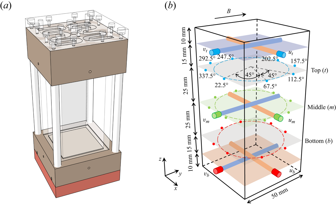
 $D = 5$ cm) Rayleigh–Bénard convection cell that was similar to the cell used in our previous experiments (Chen et al. Reference Chen, Xie, Yang and Ni2023, Reference Chen, Yang and Ni2024b), hence, we outline only the essential features here. The convection cell consists of three parts, namely, the upper cooling copper plate, the Plexiglas sidewall and the lower heating copper plate that are connected by four nylon rods as shown in figure 1(a). The upper plate was cooled by circulating temperature-controlled cooling water through two symmetrical channels machined on its backside. The cooling water was supplied by a temperature-regulated water tank with an accuracy of 0.01 K (XIATECH C3150A). The lower plate was heated by a resistance wire (OMEGA NI80-015-200). The heating power was provided by a programmable DC power supply (GWINSTEK PSW 250-13.5) with a maximum power of 1080 W. Both plates were electroplated with a thin layer of nickel to prevent the corrosion of copper by the working fluid.
(a) The schematic of the  $\varGamma =0.5$ convection cell that is composed of the upper cooling plate and the lower heating plates and a Plexiglas sidewall. (b) Positions of ultrasonic transducers to obtain the velocities and thermistors to measure the temperature distribution along the azimuthal direction. The angle corresponding to each thermistor is also marked. Here
 $u_{j}$ and
 $v_{j}$ are the velocities measured by the MPUDV. The direction of the external horizontal magnetic field is along
 $y$.
The cell is wrapped with a thermal insulation material approximately 4 cm thick and situated within a heating basin that envelops the lower plate, ensuring it maintains an equivalent temperature. This arrangement effectively reduces heat loss. Additionally, a thermostat covers the entire apparatus to mitigate the impact of ambient temperature fluctuations on convection. The thermostat is calibrated to maintain a temperature of  $35 \pm 0.5\,^{\circ }\mathrm {C}$, closely aligning with the mean temperature of the working fluid. Consequently, the use of these set-ups can effectively reduce heat leakage.
The working fluid used in this experiment is the eutectic alloy  $\mathrm {Ga}^{67}\mathrm {In}^{20.5}\mathrm {Sn}^{12.5}$, chosen for its low melting point (approximately
 $10.5\,^{\circ }\mathrm {C}$), non-toxicity and robust electrical and thermal conductivity. These characteristics render it highly suitable for liquid metal thermal convection experiments. According to previous studies (Plevachuk et al. Reference Plevachuk, Sklyarchuk, Eckert, Gerbeth and Novakovic2014, Reference Plevachuk, Sklyarchuk, Eckert, Gerbeth and Novakovic2015), the physical properties of GaInSn are varied with the temperature. In the present study we adopted the physical properties of GaInSn at a mean temperature of
 $\bar {T}=35\,^{\circ }\mathrm {C}$, therefore, the corresponding Prandtl number is 0.029. The horizontal magnetic field is generated by an electromagnet comprising two solenoids and iron cores. The strength of the magnetic field is controlled by the excitation current and the gap distance between the two iron cores. The maximum magnetic flux density can attain 0.5 T with a 300 mm gap distance. In the central
 $300\ \mathrm {mm} \times 300\ \mathrm {mm} \times 300\ \mathrm {mm}$ region of the magnetic field, the inhomogeneity is less than 5 %. With this configuration, the experimental set-up achieves parameter ranges of
 $3.8\times 10^5 \leqslant Ra \leqslant 1.1 \times 10^7$ and
 $0 \leqslant Ha \leqslant 2041$.
The temperature difference across the cell, denoted as  $\Delta T = T_{b} - T_{t}$, is measured utilizing four thermistors (OMEGA 44031) embedded in each plate, positioned 2 mm from the conducting surface to record temperatures
 $T_{t}$ and
 $T_{b}$. To reconstruct the flow structures, the multi-thermal-probe method is employed, which has demonstrated its capability to measure the dynamics of the large-scale circulation (LSC) across various cell geometries and
 $Pr$ values (Cioni et al. Reference Cioni, Ciliberto and Sommeria1997; Xi & Xia Reference Xi and Xia2008; Brown & Ahlers Reference Brown and Ahlers2009; Ren et al. Reference Ren, Tao, Zhang, Ni, Xia and Xie2022; Chen et al. Reference Chen, Xie, Yang and Ni2023). As shown in figure 1(b), in the present measurement system, 24 thermistors are strategically placed into blind holes on the sidewall to form three horizontal heights:
 $z=3H/4$,
 $z=H/2$ and
 $z=H/4$ from the lower plate. The tip of each thermistor is positioned 0.5 mm away from the surface of the liquid metal. To ensure better thermal contact, the blind holes are filled with thermally conductive paste. At each
 $z$ level, eight thermistors are equally spaced in the azimuthal direction, as indicated by the coloured dots in figure 1(b). The temperature profile at each height is modelled by
 \begin{equation} T_{i,j} = T_{0,j} + A_{j} \cos(i{\rm \pi}/4 - \theta_{j}) \quad (i=0\ldots7), \end{equation}
where  $T_{0,j}$ represents the mean temperature of the eight thermistors at one height, and
 $j=t, m$ and
 $b$ correspond to the top, middle and bottom heights of the cell, respectively. At each time step, the azimuthal temperature differences
 $A_{j}$ and the azimuthal orientation
 $\theta _{j}$ (i.e. the position where hot fluid ascends) of the LSC are determined. All 32 thermistors are measured using a multichannel multimeter (KEYSIGHT DAQ970A) with a sampling rate of 0.47 Hz.
Due to the opacity of the liquid metal, optical measurement techniques such as particle image velocimetry and laser DOPPLER velocimetry are not suitable for velocity measurement. Instead, a homemade multichannel pulsed ultrasonic Doppler velocimeter (MPUDV) is employed to acquire the velocity distributions in liquid metal (Pan et al. Reference Pan, Huang, Lyu, Yang and Ni2024). Six ultrasonic transducers with a pulse emission frequency of 8 MHz are connected to the MPUDV and mounted on two adjacent sidewalls of the cuboid convection cell to obtain the velocities in two orthogonal directions i.e.  $u$ and
 $v$ at three different layers, as illustrated in figure 1(b). At each height, the two orthogonal transducers intersect at the centre of the beamlines, facilitating the acquisition of two-dimensional velocity data at three points. The ultrasonic transducers in the top and bottom measurement layers are positioned 10 mm away from the copper plates, thereby facilitating the acquisition of more precise large-scale velocities. Based on the characteristics of the convective flow, the spatial and temporal resolutions of the velocity measurements are set to approximately 0.24 mm and 2 Hz, respectively.
Before each experimental run, the expected magnetic field is initially applied. Subsequently, based on the desired Rayleigh number, the corresponding temperature difference  $\Delta T$ is set. This ensures consistent
 $Ra$ values under varying magnetic field conditions. The temperatures of the two plates are monitored and adjusted by an in-house program. The measurement starts once the difference between the target and actual temperatures is less than 0.01 K.
3. Flow morphologies
3.1. Quasi-two-dimensional and 3-D flow morphologies
In the MC system the interplay between the Lorentz force induced by the external magnetic field and the buoyancy force originating from temperature differences plays a fundamental role in shaping flow morphology. In this part, we introduce several typical flow morphologies and their basic characteristics.
To investigate the influence of an external magnetic field on flow morphologies, three typical flow morphologies with the same  $Ra$ under different
 $Ha$ values are selected and illustrated in figure 2. The velocities along the
 $x$ and
 $y$ directions are illustrated by the blue cones in the left column of figure 2, representing the direction and magnitude of flow velocity along the velocity measurement lines. The depth of the cone's colour and the size of the cone are used to indicate the magnitude of velocity at a given point. A deeper blue colour corresponds to higher velocity, and similarly, a larger cone, particularly with a larger radius at the base, also signifies greater velocity. The measured velocity is normalized using the free-fall velocity,
 $u_{ff} = \sqrt {\alpha g \Delta T H}$. The coloured stripes on the sidewall at each height represent the azimuthal temperature distributions normalized by the mean temperature of each height and the temperature difference across the cell. Hot flow ascends near warm-coloured regions, while cold flow descends near cold-coloured regions. By analysing the temperature distribution along the sidewall in conjunction with the direction of velocity, we can accurately reconstruct the internal flow field, as illustrated by the dashed ellipses and arrows in the left column of figure 2.
Panels (a,d,g) show schematics of the 3-D single roll without oscillations ( $Ha=102, Ra=3.6\times 10^6$), 3-D single roll with oscillations (
 $Ha=209, Ra=3.6\times 10^6$) and oscillating double roll (
 $Ha=527, Ra=3.6\times 10^6$), respectively. The dashed ellipses and arrows are used to depict the flow paths conveniently. Panels (b,e,h) and (c,f,i) exhibit the corresponding space–time plots normalized by the free-fall velocity
 $u_{ff}$ and PSDs of the
 $x$ velocities measured at the three different heights. Each velocity PSD curve is scaled in intensity for identification.
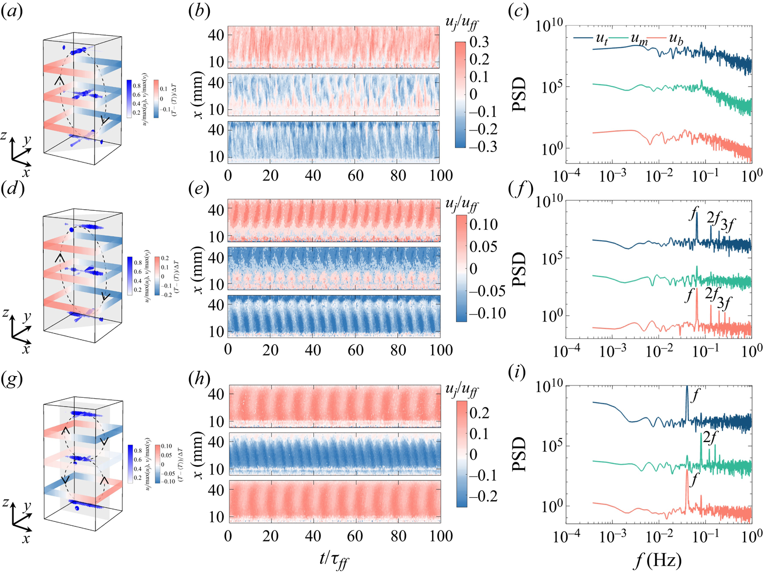
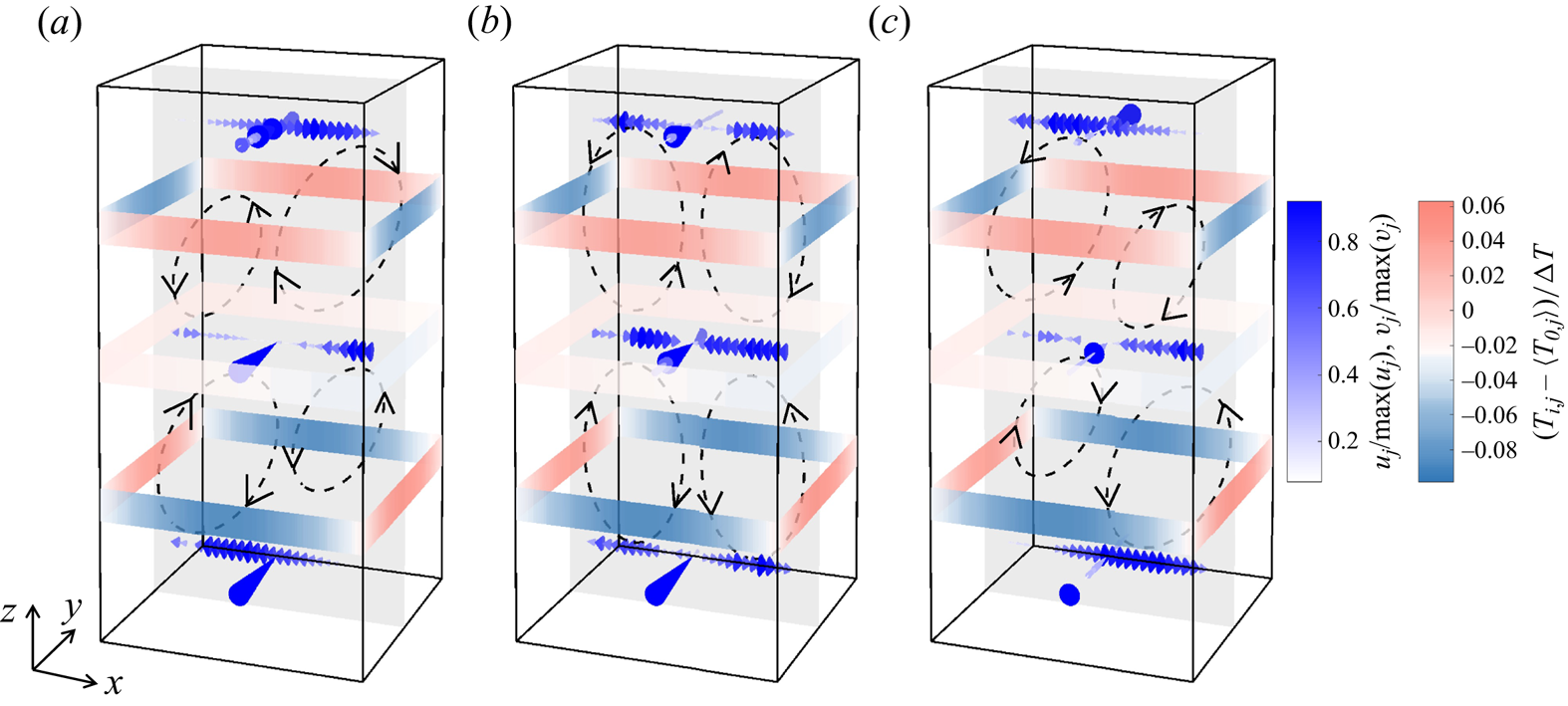
In figures 2(a)–2(c) a flow morphology called ’3-D single roll without oscillations’ (3-D SR no oscillations) is depicted. The flow exhibits some 3-D properties, such as the orientation difference between the top and bottom heights reaching up to  ${\sim }40^{\circ }$, the
 $x$ and
 $y$ velocities at the middle height have comparable magnitudes as indicated by figure 3(a) and the direction of
 $x$ velocity varies randomly with time as shown in figure 2(b). Furthermore, the convection plane is in the diagonal of the cell similar to the cases without magnetic field reported in our previous work (Chen et al. Reference Chen, Xie, Yang and Ni2023).
Time-averaged, normalized velocity profiles in the  $x$ (perpendicular to the magnetic field) and
 $y$ (parallel to the magnetic field) directions at each measurement point across three heights when (a)
 $Ra=3.6\times 10^6, Ha=102$, (b)
 $Ra=3.6\times 10^6, Ha=209$ and (c)
 $Ra=3.6\times 10^6, Ha=527$.

As  $Ha$ increases, the Lorentz force becomes more pronounced, leading to the suppression of velocities parallel to the magnetic field direction (Davidson Reference Davidson2017). With a slight increase in magnetic field strength, velocities in the
 $y$ direction are suppressed and velocities in the
 $x$ direction become dominant, as depicted in figure 2(d). Meanwhile, the convection plane remains diagonal, and the LSC shows periodic oscillations around the diagonal, as illustrated by the regular stripes in figure 2(e). The power spectral densities (PSDs) in figure 2(f) also show peaks corresponding to the oscillation frequencies and their harmonics. The peak in PSD of
 $u_{m}$ is not as sharp as the other two since the velocity in the centre of the cell is close to zero, which is a typical feature of the single-roll structure. In our experiment, we designate this flow morphology as ‘3-D single roll with oscillations (3-D SR oscillations)’. Figure 3(b) shows that the velocity parallel to the magnetic field is significantly reduced compared with the velocity perpendicular to it, reflecting the transition of the flow from three dimensional to quasi-two dimensional.
Further increases in  $Ha$ lead to a Q2-D flow morphology, where convection rolls elongate along the magnetic field direction, exhibiting strong anisotropy (Sommeria & Moreau Reference Sommeria and Moreau1982; Burr & Müller Reference Burr and Müller2002). In this state, the velocities along the direction of magnetic field vanish as shown in figure 3(c). The convection plane shifts to the centre plane of the cell, and the single-roll structure bifurcates into two rolls with opposite rotation directions, forming an oscillating double-roll (ODR) structure as shown in figure 2(g). The velocity magnitudes are enhanced in the centre of the cell, which are almost twice as large as
 $u_{t}$ and
 $u_{b}$, as shown in figure 3(c). Moreover, the oscillation frequency in the middle is also the superposition of the upper and lower parts, which can be seen from figure 2(i) in which the peak of
 $u_{m}$ is twice the oscillation frequencies of
 $u_{t}$ and
 $u_{b}$.
These flow morphologies, observed in our experiment, also appear in thermal convection experiments without a magnetic field. However, in the presence of a magnetic field, the Lorentz force modulates the conductive fluid, resulting in anisotropic and stable morphologies compared with traditional convection systems. We do not address the remaining structures, namely the Q2-D single-roll (Q2-D SR) structure and the non-oscillating stable double-roll (SDR) structure, as their main characteristics can be inferred from the typical flows discussed above.
3.2. Cellular flow
The presence of Q2-D or 3-D flow morphologies has also been noted in earlier MC systems (Yanagisawa et al. Reference Yanagisawa, Hamano, Miyagoshi, Yamagishi, Tasaka and Takeda2013, Reference Yanagisawa, Yamagishi, Hamano, Tasaka and Takeda2011; Vogt et al. Reference Vogt, Ishimi, Yanagisawa, Tasaka, Sakuraba and Eckert2018, Reference Vogt, Yang, Schindler and Eckert2021; Yang et al. Reference Yang, Vogt and Eckert2021). However, it is conceivable that the flow morphology will further differentiate at higher values of  $Ra$ and
 $Ha$. In this section, by performing a high-order Fourier expansion of the sidewall temperature coupled with instantaneous velocity data, we discovered a high-order flow mode that exhibits periodic oscillations under the action of a horizontal magnetic field.
We initially present the temperature profiles, which are the first observations leading to the discovery of this flow morphology. We have chosen the case at  $Ra=6.4\times 10^6$ and
 $Ha=1270$ as an example. In figure 4(a) the temperature variations with space and time are plotted. The temperature variations at the top and bottom heights exhibit similarities and, for convenience, we describe the phenomenon observed at the top height. Two red oscillation stripes represent the spatial location and temporal evolution of the hot flow. Unlike the common LSC, where only one hot point and one cold point are typically observed at the same height, the flow in this case exhibits a high-order Fourier flow mode (Xie, Ding & Xia Reference Xie, Ding and Xia2018; Wei Reference Wei2021; Xu, Chen & Xi Reference Xu, Chen and Xi2021; Xu, Xu & Xi Reference Xu, Xu and Xi2023). For high-order flow modes, the temperature data cannot be adequately fitted by (2.1). Instead, a second-order Fourier function is employed, defined as
 \begin{equation} T_{i,j}=T_{0,j}+\sum_{n=1}^{4}\left[a_{n,j}\cos\left(\frac{n{\rm \pi}}{4}i\right)+b_{n,j}\sin \left(\frac{n{\rm \pi}}{4}i\right)\right]\quad (i=0\ldots7), \end{equation}
here,  $n=1, 2, 3, 4$ are the
 $n$th Fourier mode and we obtain the
 $n$th Fourier mode energy as
 \begin{equation} E_{n, j}=a_{n, j}^2+b_{n, j}^2, \end{equation}
and the total energy of all modes as
 \begin{equation} E_{t,j}=\sum_{n=1}^{4}E_{n,j }.\end{equation}
(a) Space–time plot of temperature in the top height at  $Ra=6.4\times 10^6$ and
 $Ha=1270$. Two solid lines represent the azimuthal locations of the local highest temperature and the two dashed lines correspond to the azimuthal locations of the local lowest temperature. (b) Instantaneous temperature profiles measured at the top and bottom heights are fitted with second-order Fourier functions while the temperature obtained at the middle height is fitted with a first-order Fourier function. The symbols are the temperature measurement points at each height.

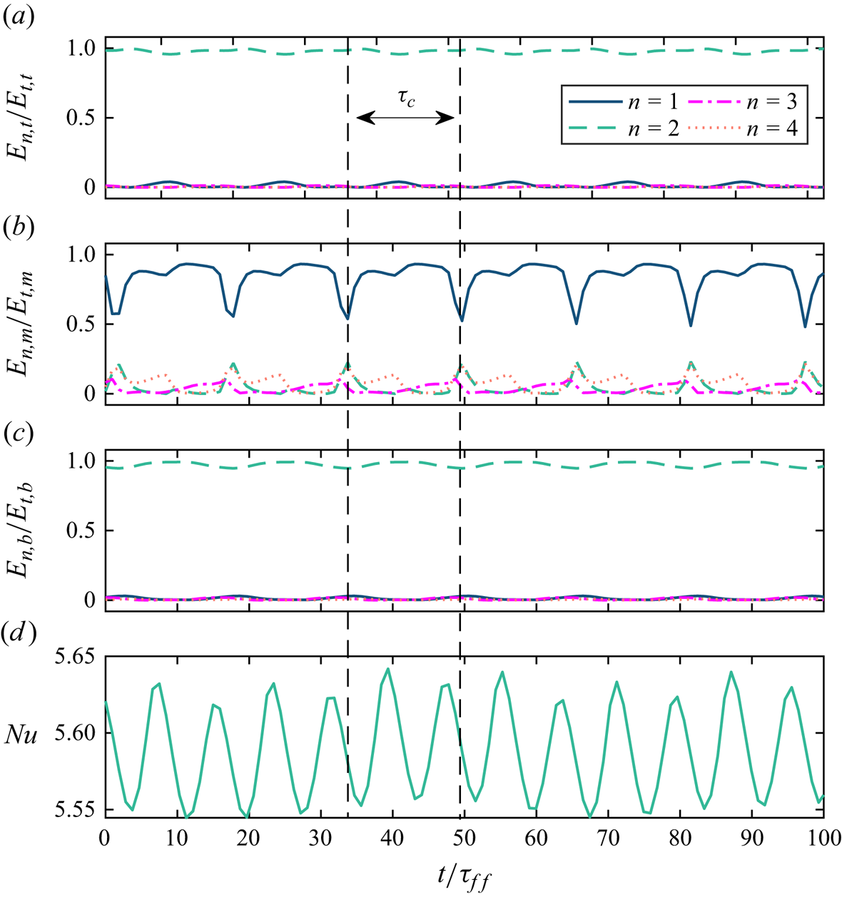
The fitting results of instant temperature profiles are illustrated in figure 4(b). Temperature profiles at both the top and bottom heights display two pairs of extreme values, consistent with a second-order Fourier function. Additionally, figure 7 reveals that the ratio  $E_{1,t}/E_{t,t}$ and
 $E_{1,b}/E_{t,b}$ are much smaller than
 $E_{2,t}/E_{t,t}$ and
 $E_{2,b}/E_{t,b}$, respectively, indicating that the second-order energy is dominant at this time. Here,
 $E_{t,t}$ and
 $E_{t,b}$ are the total Fourier mode energy of the top and bottom heights, respectively. In figure 4(b) the azimuthal angle difference between the two hottest or coldest positions is close to
 $180^\circ$, indicating that hot and cold flows occur in the central plane of the cell. The relative cold points at the top height correspond to the relative hot points at the bottom height, as depicted in figure 4(b) that is similar to the results of the four-roll state (FRS) found in Chen et al. (Reference Chen, Huang, Xia and Xi2019) and Xu et al. (Reference Xu, Chen and Xi2021). However, due to the existence of a magnetic field, this high-order flow mode can be maintained throughout the measurement process rather than in a transient or transitional state.
This peculiar temperature distribution makes us wonder how flow oscillates in cycles. Thus, combined with velocity data obtained from MPUDV measurements, the five typical  $x$ velocity profiles in an entire velocity oscillation cycle and the space–time plot of the
 $x$ velocity are obtained. The results can be seen in figure 5. The five typical velocity profiles in figure 5(a) are selected from the solid box in figure 5(b). The directions of the
 $x$ velocity at the top and bottom heights alternate with time, as illustrated in figure 5(a). Notably, at specific moments
 $\tau$, such as
 $\tau /\tau _c=0.25$ and 0.75, the velocity profiles at these heights coincide. Subsequently, the velocity directions change and then go back again. However, for the velocity at the middle height, the profiles display a similar pattern, with the velocity magnitude being positive near the ultrasonic transducers and becoming negative farther away, resembling a sinusoidal curve. In the ultrasonic velocity measurement process, the positive or negative value of the velocity indicates its direction. A positive value means the flow is moving away from the MPUDV transducer, while a negative value means the flow is moving toward the MPUDV transducer. The abnormal maximum velocity values at both ends of the velocity profile in figure 5(a) are attributed to the near-field effect of ultrasound and the refraction of ultrasound by the far-field wall.
(a) The  $x$ velocity profiles measured in three heights within an entire cycle named
 $\tau _c$ at
 $Ra=6.4\times 10^6$ and
 $Ha=1270$. The
 $x, y$ and
 $z$ axes are the locations of the MPUDV beamlines, time and the velocity magnitude, respectively. The five instants
 $\tau$ are picked from the black rectangle box in (b), the space–time plot of
 $x$ velocity at three heights. The free-fall time in this case is
 $\tau _{ff}\approx 2.262$ s.

To more intuitively observe the internal flow structure, we draw the schematics of the flow structures based on the instantaneous temperature distributions at the different heights and the velocities obtained from every measurement point. The schematics illustrating flow morphologies at three distinct moments selected from the half-oscillation cycle are depicted in figure 6. We hypothesize the existence of four elongated, Q2-D convection rolls aligned with the magnetic field direction. This inference is consistent with the higher-order flow pattern exhibited by the temperature data (Chen et al. Reference Chen, Huang, Xia and Xi2019; Xu et al. Reference Xu, Chen and Xi2021). The rotational direction of these four vortices can be determined based on the temperature distribution on the sidewall and remains constant over time. But why does the direction of velocity show a periodic reversal as plotted in figure 5(b)? We then describe the dynamic behaviour of this flow to answer this question. At the initial moment, the upper-right roll surpasses the size of the upper-left one, as evident from the predominance of larger cones on the right side along the measurement line. The counter-rotation facilitates the transport of the cold plume at the top towards the two opposing sidewalls, leading to the formation of two localized low-temperature points with an azimuthal angle difference of  $180^\circ$. This observation is consistent with the findings displayed in figure 4(b). A similar scenario unfolds in the lower part of the cell, where the hot plume at the bottom is likewise transported toward the two opposing sidewalls by the counter-rotating rolls. The flow is fully mixed by the four rolls leading to a more uniform temperature distribution at the middle height, thus, the normalized temperature fluctuations approach zero, as indicated by the light-coloured stripes. These findings align with the instantaneous temperature profiles of the middle height, as illustrated in figure 4(b), where the eight temperature data points consistently maintain similar values, approximately around
 $35^\circ \mathrm {C}$, i.e. the mean temperature of the fluid. The temperature measurement points at the middle height can be fitted by (2.1) well, which is the reason for the dominance of
 $E_{1,m}/E_{t,m}$ in figure 7(b).
The schematics of cellular flow morphology at  $Ra=6.4\times 10^6$ and
 $Ha=1270$. From (a–c) are the three typical instants,
 $\tau /\tau _c=0$,
 $\tau /\tau _c=0.25$ and
 $\tau /\tau _c=0.5$, respectively. The shaded area is one of the slices of the flow field, here the central plane is chosen. The dashed ellipses and arrows are drawn to visualize the vortices.
Time series of four Fourier mode energy ratios for (a) top, (b) middle and (c) bottom heights. Additionally, (d) shows the corresponding time series of  $Nu$ at
 $Ra=6.4\times 10^6$,
 $Ha=1270$.
The schematic of the flow field at  $\tau /\tau _c=0.25$ is shown in figure 6(b). At this time, the sizes of the four rolls become comparable, allowing the detection of two main movements in opposite directions by the MPUDV. In this scenario, the velocities at the top and bottom heights exhibit similar patterns. It should be noted that the rotation direction of each roll does not change and, as a result, the temperature distributions on the sidewalls also remain unchanged. As time goes by, the size of each roll in figure 6(b) starts to change the opposite way compared with the change from
 $\tau /\tau _c=0$ to
 $\tau /\tau _c=0.25$. Therefore, the upper-right roll begins to compress while the upper-left roll expands, ultimately dominating the corresponding velocity measurement line, resulting in a velocity reversal compared with that shown in figure 6(a). The interplay between the mutual compression deformation of multi-roll structures may be correlated with the dynamics of vortices (Aref & Zawadzki Reference Aref and Zawadzki1991).
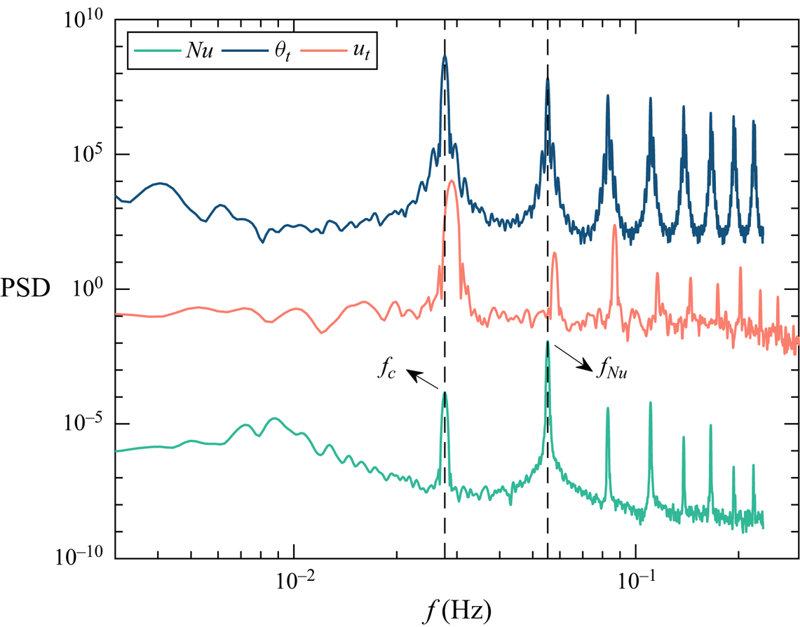
The multi-roll morphology undergoes stable changes over time, characterized by an oscillation frequency  $f_c$, as depicted in figure 8. In this instance, with
 $f_c \approx 0.027$ Hz, the associated time scale
 $\tau _{c}$ approximates 37.03 s, roughly 16.4
 $\tau _{ff}$, where
 $\tau _{ff}=\sqrt {H/(g \alpha \Delta T)}$ is the free-fall time of the thermal convection, indicating a long-term dynamical behaviour. In figure 8 the frequencies corresponding to the PSD peaks are higher for
 $u_t$ (about 0.029 Hz) compared with
 $Nu$ and
 $\theta _t$. This discrepancy can be attributed to asynchrony issues arising from different measurement techniques, but the offset is small and within an acceptable range. As a consequence of this oscillation, the temperature on the sidewall also exhibits periodic fluctuations with the same frequency indicated by the PSD of
 $\theta _t$ in figure 8. However, there are noticeable differences in the PSD of
 $Nu$ and its time series in figure 7(d). The primary peak frequency of
 $Nu$, denoted as
 $f_{Nu}$, is twice that of
 $f_{c}$. This discrepancy is evident in figure 7(d), where the peaks of
 $Nu$ display bimodal characteristics, featuring one higher peak and one lower peak. The bimodal behaviour of
 $Nu$ stems from the distinct stages of vortex morphology changes.
Power spectra density of  $Nu$,
 $\theta _{t}$ and the velocity
 $u_{t}$ at
 $Ra=6.4\times 10^6$,
 $Ha=1270$. To avoid overlapping of PSD curves, we multiply each PSD curve by a specific constant so that they are separated from each other on a logarithmic scale.
Typically, velocity reversal in the RBC system is commonly associated with either the merging of corner rolls (Chen et al. Reference Chen, Huang, Xia and Xi2019; Chen, Wang & Xi Reference Chen, Wang and Xi2020) or the massive eruption of thermal plumes (Wang et al. Reference Wang, Lai, Song and Tong2018). In the MC system, a well-known flow reversal in the cell with large  $\varGamma$ is attributed to a reorganization process of the roll-like structures (Yanagisawa et al. Reference Yanagisawa, Yamagishi, Hamano, Tasaka and Takeda2011; Tasaka et al. Reference Tasaka, Igaki, Yanagisawa, Vogt, Zuerner and Eckert2016; Chen et al. Reference Chen, Wang and Ni2024a). However, in our experiments, the velocity reversal shown in the space–time plot of figure 5 is attributed to variations in the dominant velocity along the measurement line, resulting from changes in the relative sizes of multiple rolls, rather than a counter-rotation of the flow. Here, a novel high-order flow morphology and its dynamics are presented. Recognized for its distinctive multi-roll structure, we refer to this flow morphology as ‘cellular flow’. Zürner et al. (Reference Zürner, Schindler, Vogt, Eckert and Schumacher2020) also observed a ‘cellular’ structure; however, their configuration extends throughout the entire container in three dimensions, whereas the cellular flow investigated in our study is confined to the plane perpendicular to the magnetic field maintaining a Q2-D form. Additionally, their experiment was conducted under the influence of a vertical magnetic field, which differs from the direction of the magnetic field in our study.
3.3. Regime map
All the flow regimes are summarized in figure 9. The entire parameter space is divided into five distinct regimes (i.e. conduction, steady, periodic, cellular and chaotic), classified based on their flow morphologies or flow features.
Regime map over the ( $Ra, Ha$) parameter space. The coloured regions are the four flow regimes separated by a dash-dotted line (
 $Ha=Ra/400$), dashed line (
 $Ha=Ra/1600$) and a dotted line (
 $Ha=Ra/10\,000$), respectively. For details of the twisted LSC in the figure, we refer the reader to Chen et al. (Reference Chen, Xie, Yang and Ni2023).

In the conduction regime, in the presence of a strong magnetic field, the ratio between buoyancy force and Lorentz force is much less than 1, i.e.  $Ra/Ha^2 \ll 1$. Due to the lack of buoyancy-driven force, the convection is somewhat suppressed, and heat transfer in these cases primarily relies on heat conduction, leading to
 $Nu \approx 1$. A stagnation of the flow occurs, consequently termed ‘stagnant flow (SF)’. In this regime the flow velocities are below the measurement limit of the MPUDV and, therefore, the velocity measurement results are not discussed. As
 $Ha$ and
 $Ra$ cross the dash-dotted line (i.e.
 $Ha=Ra/400$) in figure 9, the flow enters the so-called steady regime characterized by the predominance of a ’Q2-D SR’, where the convection plane aligns with the direction of the magnetic field. The characteristics of a Q2-D SR are similar to the Q2-D convection rolls elongated in the direction of the magnetic field observed in the MC system, as reported in some previous work with large
 $\varGamma$ (Yanagisawa et al. Reference Yanagisawa, Yamagishi, Hamano, Tasaka and Takeda2011, Reference Yanagisawa, Hamano, Miyagoshi, Yamagishi, Tasaka and Takeda2013; Vogt et al. Reference Vogt, Yang, Schindler and Eckert2021; Yang et al. Reference Yang, Vogt and Eckert2021; Chen et al. Reference Chen, Wang and Ni2024a). Therefore, we decide not to discuss this in detail here.
Considering the steady flow structure of a Q2-D SR, the magnetic field effect remains crucial in this regime. As  $Ra$ increases, the initially steady single-roll structure, influenced by the growing buoyancy force, undergoes instability due to the small
 $\varGamma$ (Zwirner et al. Reference Zwirner, Tilgner and Shishkina2020), transformed into two rolls stacked on each other (e.g. SDR and ODR structures) or multiple rolls (e.g. cellular flow), as depicted in figures 2(g) and 6. The double-roll structure undergoes periodic oscillations over time within this parameter range, thus, we designate this regime as the periodic regime. Additionally, the cellular flow occupies a significant portion of the parameter space and also shows obvious periodic behaviours. Consequently, we hereby refer to the region where the cellular flow predominates as the cellular regime. Examining the regime map reveals that the cellular flow not only emerges in the cellular regime with large
 $Ha$ and
 $Ra$ but also in cases near the dotted line, i.e. the boundary between periodic and chaotic regimes. Hence, we speculate that the cellular structure originates from the double-roll structure. However, it is subjected to a stronger buoyancy force than the double-roll structure, characterized by a larger
 $Ra$. This leads to either the splitting of the double-roll structure or the growth of corner vortices, ultimately resulting in a multiple-roll structure. Furthermore, the brief occurrences of the twisted LSC structure, as reported by Chen et al. (Reference Chen, Xie, Yang and Ni2023), are denoted by cross symbols. Remarkably, the twisted LSC structure is exclusively observed at
 $Ha = 209$, potentially owing to the weak magnetic field constraint and its proximity to the transition line between the two flow regimes.
The final regime, denoted as the chaotic regime, is primarily characterized by large-scale ‘3-D single-roll (3-D SR) structures’, with its convection plane located on the diagonal of the cell, a configuration similar to that observed without a magnetic field. In this regime the buoyancy-driven effect significantly outweighs the magnetic field suppression effect, i.e.  $Ra/Ha^{2}\gg 1$. Moreover, there is no clear boundary to distinguish the oscillating characteristics of a 3-D SR. The reappearance of velocity in the
 $y$ direction serves as evidence of the three-dimensionality of the flow, as depicted in figure 2(a).
4. Results of flow characteristics
In the preceding sections we discuss various flow morphologies that arise under the influence of a horizontal magnetic field, organizing the entire parameter space according to these morphologies. In this part we examine the flow characteristics across different flow regimes.
4.1. Azimuthal temperature difference and temperature gradient
Using the multi-thermal-probe method illustrated in § 2, the azimuthal temperature difference of each height can be easily obtained from the rows of thermistors at the three heights. In (2.1),  $A_{j}$ describes the temperature difference between hot and cold plumes at each height, thereby reflecting the flow strength at that altitude to a certain extent.
In figure 10, normalized azimuthal temperature differences are plotted against  $Ra$ for three different magnetic field strengths, with distinct flow regimes distinguished by colour. Within the steady regime characterized by a Q2-D SR structure, flow strengths at different heights exhibit proximity, as depicted in the corresponding flow regimes in figures 10(b) and 10(c). As the
 $Ra$ gradually nears the critical
 $Ra$ for transitioning between the steady and periodic regimes, flow strengths across the three layers experience a moderate decline, which can be considered a sign that instability is beginning to take effect. The distinct jump of
 $A_{m}/\Delta T$ observed in the periodic regime in figure 10(a) is attributed to the twisted LSC structure described in our previous work (Chen et al. Reference Chen, Xie, Yang and Ni2023).
Azimuthal temperature difference normalized by the system temperature difference  $\Delta T$ as a function of
 $Ra$ for different
 $Ha$ and flow regimes. Results are shown for (a)
 $Ha = 209$, (b)
 $Ha = 527$ and (c)
 $Ha = 1270$.

Distinct differentiation in azimuthal temperature difference across the three heights becomes apparent within the periodic regime. Here, the prevalent double-roll structure manifests prominently, with the azimuthal temperature difference at the middle height notably diminishing, approaching zero. This phenomenon arises due to the contact of the two counter-rotating vortices in the middle, leading to their mutual interaction and temperature homogenization, thereby resulting in a low-intensity region.
In the chaotic regime the flow structure resembles the large-scale flow observed in the absence of a magnetic field. While some deviations in azimuthal temperature difference exist across the three heights, as depicted in figures 10(a) and 10(b), it remains relatively small. This observation aligns with findings in the RBC system (Xi & Xia Reference Xi and Xia2008; Weiss & Ahlers Reference Weiss and Ahlers2011). Notably, within the cellular regime as shown in figure 10(c), flow strengths at three heights converge closely, albeit significantly smaller in magnitude compared with the single-roll structure. This reduction in strength stems from the extremely lower first-order mode energy of the flow mentioned before, leading to an overall decrease in azimuthal temperature difference.
The quantity  $\delta T_{b, t} = 2\langle T_{0, b}-T_{0,t}\rangle _{t}/\Delta T$ represents the vertical temperature gradient near the sidewall. Here,
 $T_{0, b}$ and
 $T_{0, t}$ correspond to the mean temperatures at the bottom and top heights, respectively;
 $\langle \dots \rangle _{t}$ indicates the average over time. The temperature gradient provides another perspective to measure the influence of flow structure on the overall temperature change of the system (Brown & Ahlers Reference Brown and Ahlers2007). Figure 11 illustrates the sidewall temperature gradients corresponding to
 $Ha$, as plotted in figure 10. It is evident that for the double-roll structure (primarily in the periodic regime), the temperature gradients are significant, indicating substantial temperature discrepancies between the upper and lower parts of the cell, and suggesting inadequate heat transport within the system. Conversely, for the single-roll structure, as
 $Ra$ increases, the temperature gradient notably decreases, as depicted in the steady regime in figures 11(b) and 11(c). In cellular flow the temperature gradient is smaller compared with that of the double-roll structure and shows minimal dependence on the
 $Ra$ number, as depicted in figure 11(c).
Normalized sidewall temperature gradient  $\delta T_{b,t}$ vs
 $Ra$ for different
 $Ha$ and flow regimes. Results are shown for (a)
 $Ha = 209$, (b)
 $Ha = 527$ and (c)
 $Ha = 1270$.

To comprehensively examine the relationship between the temperature gradient and both the  $Ra$ number and
 $Ha$ number, we normalized the temperature gradient in different regimes. The free-fall interaction parameter
 $N_{ff} = Ha^{2}/Re_{ff}$ that quantifies the ratio of magnetic and buoyant forcing in the fluid (Zürner et al. Reference Zürner, Schindler, Vogt, Eckert and Schumacher2020) is introduced, where
 $Re_{ff} =(Ra/Pr)^{1/2}$. The dependence of
 $\delta T_{b, t}$ can be described by
 \begin{equation} \delta T_{b, t}^{ \beta}=\gamma \frac{Ha}{N_{ff}^{\alpha}}. \end{equation}
The dashed lines represent the least-squares fits to the data, with the corresponding parameters  $\alpha$,
 $\beta$ and
 $\gamma$ displayed in figure 12 for each regime. The fitting uncertainties for the three parameters are calculated based on the 95 % confidence interval. For each fitting line, the coefficient of determination (
 $R^2$) is greater than 0.95, indicating good fitting accuracy. Utilizing (4.1) for data fitting demonstrates a notable collapse of the data within each respective regime. The
 $\alpha$ values obtained through fitting are consistent, ranging from 0.5 to 0.6 across all regimes. Therefore, the main difference in
 $\delta T_{b,t}$ under different flow regimes lies in the values of
 $\gamma$ and
 $\beta$ fitted in each regime. Remarkably, within the periodic regime, the smallest
 $\beta$ values are observed, suggesting that the double-roll structure manifests the most significant temperature gradient within the experimental parameter range. In contrast, within the cellular regime, the
 $\beta$ value approximates 0, implying a relatively uniform distribution of temperature gradients around 1. This observation suggests that in the cellular regime, there is minimal sensitivity of temperature gradients to both the Hartmann number and the Rayleigh number. Through data fitting, it becomes evident that a consistent mechanism underlies the variations in temperature gradients within each flow regime.
Normalized sidewall temperature gradient  $\delta T_{b,t}^{\beta }$ vs
 $Ha/N_{ff}^{\alpha }$ for different flow regimes. The dashed lines are the best-fitted lines with a coefficient of determination (
 $R^2$) greater than 0.95. The exponents
 $\alpha$ and
 $\beta$ for each regime are labelled.

4.2. Flow oscillation characteristics
Regularly oscillating flows are a common and significant aspect of MC systems. In this experiment, flow oscillation primarily occurs in the periodic, cellular and chaotic regimes. Within these regimes, the oscillations of double-roll and multi-roll structures are predominant. The oscillation frequency of the 3-D single roll observed in the chaotic regime does not show a clear monotonic increase or decrease to the  $Ra$ or
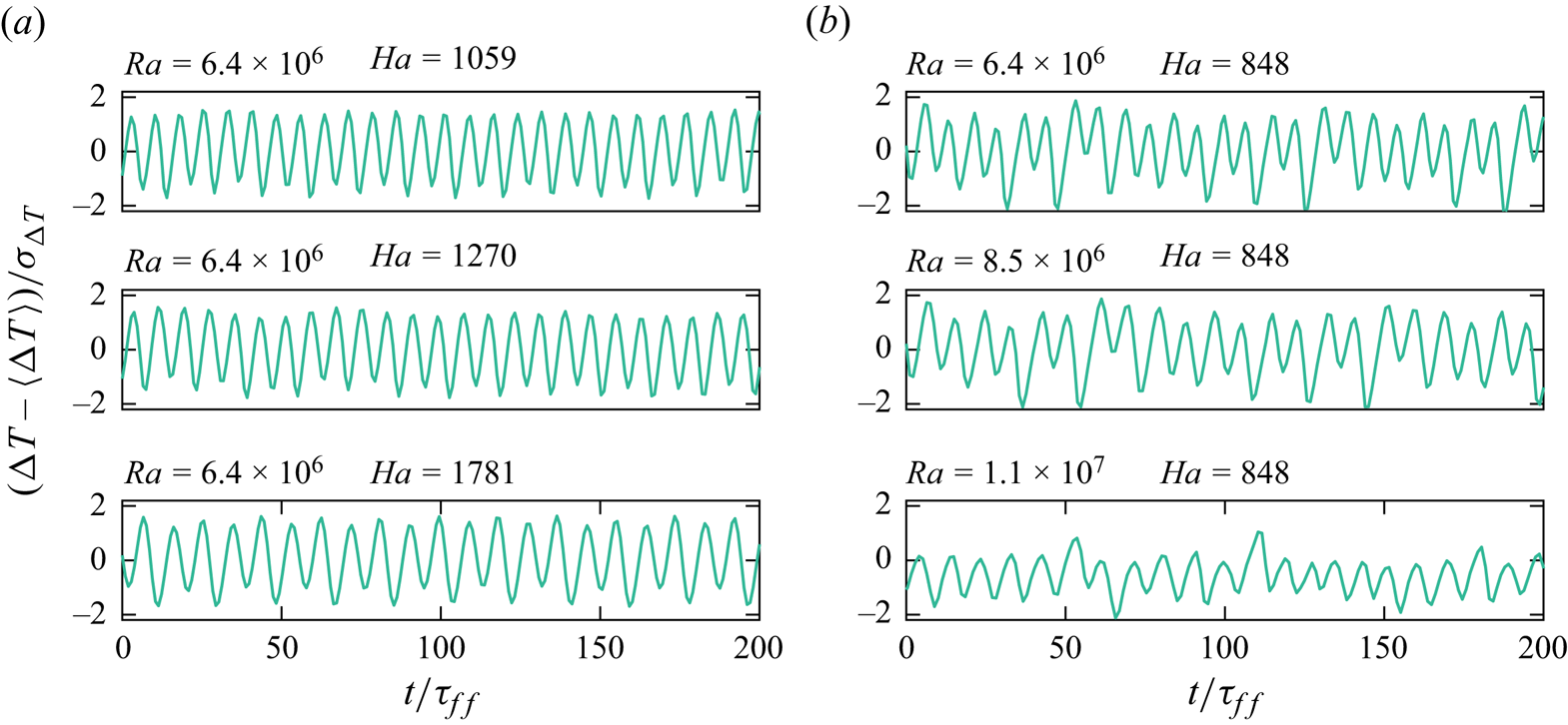
 $Ha$ numbers. Therefore, this section focuses on exploring flow oscillation behaviour under double-roll and multi-roll structures. To comprehensively observe oscillations within the convection cell, we chose to analyse the time series of the temperature difference
 $\Delta T$ between the upper and lower plates. Figures 13 and 14 present the normalized
 $\Delta T$ between the upper and lower plates, illustrating changes in the time series by increasing
 $Ha$ from a fixed
 $Ra$ number and by increasing
 $Ra$ from a fixed
 $Ha$. Figure 13(a) indicates that for the double-roll structure, an increase in
 $Ha$ reduces the oscillation frequency, while figure 13(b) shows that an increase in
 $Ra$ increases the oscillation frequency. This illustrates the competition between buoyancy and Lorentz forces. Furthermore, it is evident that regardless of changes in
 $Ha$ or
 $Ra$, the oscillation amplitude remains relatively stable, concentrated within the
 $[-2, 2]$ interval. From this, it can be inferred that the Lorentz force and buoyancy force mainly modulate the double-roll structure oscillation by altering its frequency, with little effect on its oscillation amplitude. It should be noted that figure 13(b) also displays a period-doubling phenomenon. This is related to the fact that, as
 $Ra$ increases, the flow in the periodic regime gradually transitions into the chaotic regime. This path of transition to chaos is also illustrated in figure 9. However, in the cellular regime, the scenario differs. Figure 14 demonstrates that the oscillation frequency of the multi-roll structure remains relatively unchanged with variations in
 $Ra$ and
 $Ha$, which is also evident from the inset of figure 15(b).
Time series of normalized temperature differences for the periodic regime. (a) At fixed  $Ra=4.8\times 10^6$ with increasing
 $Ha$ and (b) at fixed
 $Ha=848$ with increasing
 $Ra$.

Time series of normalized temperature differences for the cellular regime. (a) At fixed  $Ra=6.4\times 10^6$ with increasing
 $Ha$ and (b) at fixed
 $Ha=848$ with increasing
 $Ra$.
Normalized flow oscillation frequencies  $f/f_{J}$ as a function of
 $Ha/Ra$ for (a) the periodic regime and (b) the cellular regime. The dashed lines are given by a least-squares fitting of
 $(f/f_{J})^{\beta }=\gamma (Ha/Ra^{\alpha })$ applied to the data with a coefficient of determination greater than 0.95. The fitted parameters
 $\alpha$ and
 $\beta$ are indicated in the figure. The oscillation frequencies of the cellular regime without being normalized are plotted in the inset of (b).

To explore the relationship between oscillation frequency  $f$ and
 $Ha$ and
 $Ra$, we introduce the Joule dissipation time scale
 $\tau _{J}$ and its reciprocal, the Joule dissipation frequency
 $f_{J}$, as characteristic frequencies to render the oscillation frequency dimensionless. Here
 $\tau _{J}$ and
 $f_{J}$ are defined as
 \begin{equation} \tau_{J}=\frac{\rho}{\sigma B^2} \quad \text{and} \quad f_{J}=\frac{1}{\tau_{J}}= \frac{\sigma B^2 }{\rho}. \end{equation}
It is evident from figure 15 that for both double-roll and multi-roll structures, their oscillation frequencies exhibit scaling relationships with the combination of  $Ha$ and
 $Ra$, namely
 $(f_{periodic}/f_{J})\sim (Ha^{-2.33}Ra^{0.79})$ and
 $(f_{cellular}/f_{J})\sim (Ha^{-2.17}Ra^{0.41})$, respectively. In these two fitting relationships, the exponential signs of
 $Ha$ and
 $Ra$ are opposite, emphasizing the inhibitory effect of the magnetic field and the promoting effect of buoyancy on the oscillation frequencies.
5. Global transport properties
In the MC system the continuous increase in magnetic field strength tends to induce a more Q2-D flow behaviour. During this phase, the primary manifestation of the magnetic field's damping effect is Hartmann braking, where the magnetic field opposes the motion of the conducting fluid, reducing flow velocity and affecting momentum transport. Additionally, introduced Joule dissipation also leads to the conversion of kinetic energy into heat, impacting the overall thermal behaviour of the system. Certainly, a previous study conducted by Vogt et al. (Reference Vogt, Yang, Schindler and Eckert2021) has indicated that within a specific range of magnetic field strength, the self-organized structure of the flow reaches an optimal state. In this case, heat transport efficiency is augmented and the convective velocity approaches its theoretical limit, i.e. the free-fall velocity  $u_{ff}$. Only when the magnetic field intensity surpasses a certain threshold that the Hartmann braking effect becomes notable. However, it should be noted that in the present experiment, the maximum measured velocity value does not reach
 $u_{ff}$. Moreover, alterations in flow structure also significantly impact transport efficiency. In this section we primarily investigate the influence of the magnetic field on the Nusselt number and Reynolds number, which respectively represent heat and momentum transport efficiency. We also delve into the effects of flow morphologies on these parameters.
We begin our discussion of heat transport by examining the relationship between  $Nu$ and
 $Ra$ across different flow regimes. In figure 16(a) we observe variations in the
 $Nu$ number within the conduction and steady regimes. The
 $Nu$ reduces with the increase of magnetic field at fixed
 $Ra$, indicating a pronounced suppression of heat transfer with increased magnetic field strength. Especially, when the magnetic field attains significant strength, such as
 $Ha=1781$ (
 $B=0.43 T$) and
 $2041$ (
 $B=0.50 T$),
 $Nu$ approaches 1 at small
 $Ra$, indicating heat transfer predominantly occurs via thermal conduction. As
 $Ra$ increases,
 $Nu$ across different
 $Ha$ gradually converge, suggesting an asymptotic relationship,
 $Nu \sim Ra^{1/4}$. These asymptotic trends align well with theoretical predictions (Grossmann–Lohse (GL) theory) of the RBC system in the absence of a magnetic field, particularly at very low Prandtl numbers (Grossmann & Lohse Reference Grossmann and Lohse2000; Stevens et al. Reference Stevens, van der Poel, Grossmann and Lohse2013). In the inset of figure 16(a) the heat transport results without a magnetic field,
 $Nu_0$, show good agreement with Grossmann–Lohse theory. The dashed lines in figure 16 are only used as asymptotic lines, thus, we only mark their exponents, not the corresponding perfectors. This convergence can be attributed to significant buoyancy effects and the emergence of Q2-D SR structures at higher
 $Ra$ numbers, similar to the LSC observed in the RBC system.
The relationship between  $Nu$ and
 $Ra$ is examined under various
 $Ha$. The data are plotted according to distinct flow regimes: (a) conduction and steady regimes, (b) periodic regime, (c) cellular regime and (d) chaotic regime. The dashed lines represent the asymptote of the data. The inset in (a) shows the relationship between
 $Nu_0$ and
 $Ra$ in the normal LSC structure without the influence of a magnetic field.
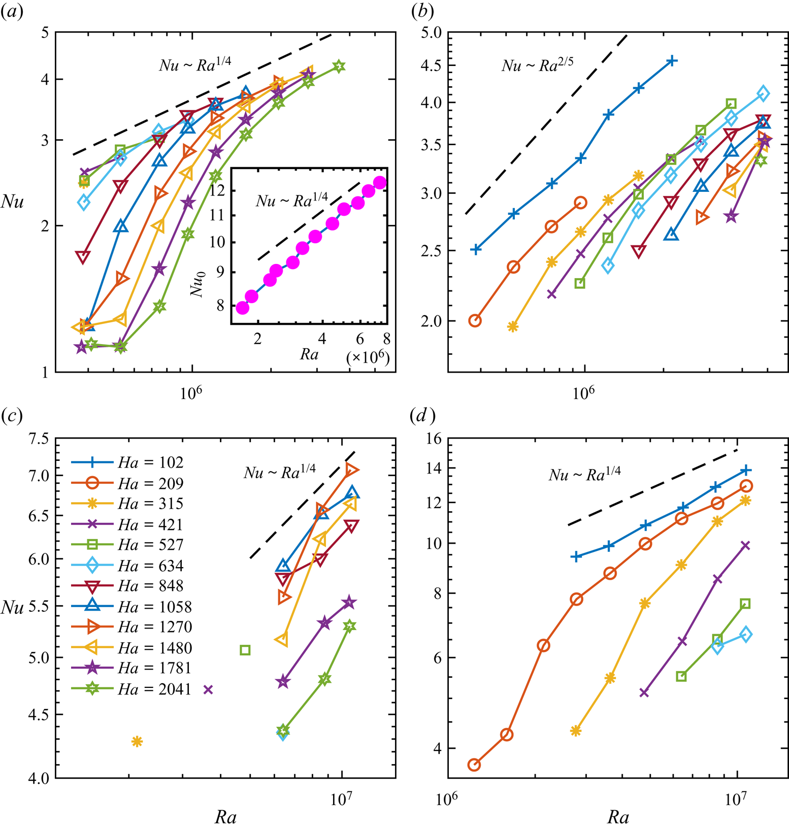
In the periodic regime (figure 16b),  $Nu$ exhibits a relatively consistent scaling relationships with
 $Ra$ across varying magnetic field strengths. Similarly, a scaling relationship approximating
 $Nu \sim Ra^{2/5}$ is fitted in this regime. In the cellular regime (figure 16c), proximity to the critical curve between periodic and chaotic regimes, particularly under weak magnetic fields, yields distinctive
 $Nu$ distributions compared with strong magnetic field scenarios. Under strong magnetic fields,
 $Nu$ exhibits an increasing trend with rising
 $Ra$, following a scaling law of
 $Nu \sim Ra^{1/4}$. It is important to highlight a significant observation from Chen et al. (Reference Chen, Huang, Xia and Xi2019) and Xu et al. (Reference Xu, Chen and Xi2021), which suggest that the FRS demonstrates comparatively lower heat transfer efficiency than the single-roll structure for water. However, in our experimental investigations involving liquid metals under the influence of magnetic fields, the multi-roll structure does not appear to significantly diminish heat transfer efficiency. Remarkably,
 $Nu$ associated with this multi-roll structure closely matches the extrapolated
 $Nu$ observed in the steady regime. This can be attributed to the excellent thermal conductivity of the liquid metal and the increased coherence of the flow structure in the presence of a magnetic field. Lastly, within the chaotic regime (figure 16d), buoyancy effects intensify, manifesting distinct 3-D large-scale flow structures. Consequently,
 $Nu$ numbers tend to approach a function of
 $Nu\sim Ra^{1/4}$ again.
In this part, we found that except for the periodic regime,  $Nu$ in other regimes tends to follow the scaling law
 $Nu\sim Ra^{1/4}$ obtained without the magnetic field. The impact of introducing a magnetic field on heat transfer results across different flow regimes is elucidated. This comprehensive analysis sheds light on the intricate interplay between magnetic field strength,
 $Nu$, and
 $Ra$ across various flow regimes.
As discussed in § 4.1, the presence of a double-roll structure creates a region of low azimuthal temperature difference in the centre of the cell, consequently amplifying the temperature differences between the upper and lower parts of the system. These phenomena contribute significantly to the reduction in heat transport efficiency. Thus, our primary focus lies in understanding the maximum reduction attributable to the double-roll structure in contrast to a single-roll configuration, and how this reduction correlates with  $Ha$.
In figure 17(a) we illustrate the transition of  $Nu$ from the steady regime to the periodic regime across several typical
 $Ha$. It is evident from the figure that
 $Nu$ initially increases with increasing
 $Ra$, experiences a sharp decline post transition and subsequently increases with further increases in
 $Ra$. To quantify the extent of the decline in
 $Nu$, we conduct a fit of
 $Nu$ and
 $Ra$ within the steady regime preceding the regime transition across different
 $Ha$. This fitting yields an extrapolated scaling relationship,
 $Nu_{ext}\sim Ra^{0.26}$, which we use to calculate
 $Nu_{ext}$ corresponding to the initial
 $Ra$ post-regime transition. We then compare this with
 $Nu_{t}$ corresponding to the double-roll structure at the same
 $Ra$ number. The findings are presented in figure 17(b). As illustrated in the figure, the regime transition can lead to a maximum reduction in
 $Nu$, up to 36 %. Compared with the heat transfer reduction caused by the double-roll structure in the RBC system with water or liquid metal (Xi & Xia Reference Xi and Xia2008; Weiss & Ahlers Reference Weiss and Ahlers2011; Chen et al. Reference Chen, Yang and Ni2024b), the double-roll structure exhibits a more pronounced inhibitory effect on heat transfer in the MC system. Furthermore, this reduction amplifies with increasing
 $Ha$, following a power-law relationship:
 \begin{equation} (Nu_{ext}-Nu_{t})/Nu_{ext} \simeq (0.11\pm0.07)Ha^{0.15\pm0.09}. \end{equation}
(a) The drop of  $Nu$ data from the steady regime to the periodic regime under several typical
 $Ha$. The dashed line is the fitting result of the critical
 $Nu$ and
 $Ra$ for regime transition. (b) Relative reduction of
 $Nu$ during regime transition.

We employ a normalization method akin to the approach used for normalizing the temperature gradient  $\delta T_{b,t}$ to standardize the
 $Nu$ across different flow regimes. We define the dependence of
 $Nu(Ha, Ra, Pr)$ as follows:
 \begin{equation} Nu^{\beta} = \gamma \frac{Ha}{N_{ff}^{\alpha}}. \end{equation}
The parameters  $\alpha$ and
 $\beta$ are fitted for each flow regime, as indicated in figure 18, and exhibit excellent data collapse. Notably, the fitted
 $\alpha$ values are consistent across various flow regimes, approximating 3/5. Except for the periodic regime, the
 $\beta$ values derived from fitting the other three flow regimes hover around 1/2. Consequently, we propose a unified scaling relationship applicable across a wide range:
 \begin{equation} Nu \sim (Ha^{{-}2/3}RaPr^{{-}1})^{3/5}. \end{equation}
Plot of  $Nu^{\beta }$ vs
 $Ha/N_{ff}^{\alpha }$ for different flow regimes. The dashed lines are the best-fitted lines. The exponents
 $\alpha$ and
 $\beta$ for each regime are labelled.

However, a satisfactory theoretical derivation of this result is currently lacking. It is anticipated that further research will delve into this aspect to provide a deeper understanding.
Before the discussion of momentum transport, we must introduce our method for processing velocity data. The velocity at different heights comprises  $v_{j}$ along the direction of the magnetic field and
 $u_{j}$ orthogonal to the magnetic field direction, where
 $j=t, m, b$. The specific arrangement of the ultrasonic transducers is illustrated in figure 1(b). Each ultrasonic transducer captures a time series of 206 measurement points along the ultrasound beam line. To mitigate discontinuities in velocity profiles and address issues arising from ultrasonic scattering due to tracer particles, we employ spatial and temporal moving average filters. Specifically, we utilize a spatial window of 2 mm (equivalent to 10 contiguous measurement points, representing approximately 5 % of the total 206 measurement points that can ensure the realistic velocity fluctuations), and a temporal window spanning five consecutive moments (about 0.05 % of the total acquisition time) to eliminate erroneous data points from the raw velocity data. The above velocity data processing is similar to Zürner et al. (Reference Zürner, Schindler, Vogt, Eckert and Schumacher2020).
According to different flow morphologies, the maximum velocity is concentrated in the central part of the velocity measurement line; thus, we select the middle part of the velocity profile as the characteristic velocity in each direction, which is defined as
 \begin{equation} \bar{u}_{j}(t) = \langle u_{j}(i, t) \rangle_{{-}D/10 \leqslant i \leqslant D/10}. \end{equation}
The same method is applied to obtain  $\bar {v}_{j}(t)$. The resulting two-dimensional velocity at each height is calculated as
 \begin{equation} U_{j}(t) = \sqrt{\bar{u}_{j}(t)^2 + \bar{v}_{j}(t)^2}. \end{equation}
Consequently, the time-averaged global large-scale velocity is defined as
 \begin{equation} U_{global} = \frac{\langle U_{t} \rangle_{t} + \langle U_{b} \rangle_{t}}{2}, \end{equation}
where  $\langle \dots \rangle _{t}$ denotes averaged over time. The corresponding global
 $Re$ is calculated as
 \begin{equation} Re = \frac{U_{global}H}{\nu}. \end{equation}
For the analysis of momentum transport, we also employ a method that distinguishes between various flow regimes. In figure 19(a), similar to  $Nu$ in the steady regime,
 $Re$ asymptotically approaches the scaling relationship without a magnetic field, i.e.
 $Re \sim Ra^{1/2}$ (Grossmann & Lohse Reference Grossmann and Lohse2000; Stevens et al. Reference Stevens, van der Poel, Grossmann and Lohse2013). This asymptotic scaling is also observed for flows in the chaotic regime, as illustrated in figure 19(d). This suggests that heat and momentum transport in these two regimes are coupled, akin to scenarios without a magnetic field. The introduction of the magnetic field, for these two flow regimes, only delays the flow to reach the Rayleigh number of the flow state without a magnetic field.
The relationship between  $Re$ and
 $Ra$ is examined under various
 $Ha$. The data are plotted according to distinct flow regimes: (a) conduction and steady regimes, (b) periodic regime, (c) cellular regime and (d) chaotic regime. The dashed lines represent the asymptote of the data.

In the periodic regime, as shown in figure 19(b),  $Re$ exhibits similarities with
 $Nu$ in figure 16(b), both possessing large scaling exponents and increasing rapidly with increasing
 $Ra$. There is no decrease in the global Reynolds number during the transition from the steady regime to the periodic regime, indicating that the behaviours of
 $Re$ and
 $Nu$ are decoupled during the transition. This is because when the flow morphology changes from a single-roll to a double-roll structure, only the flow morphology bifurcates, but the velocities at the top and bottom can still be maintained, and the momentum in the system will not be weakened by the low-intensity area generated in the middle part of the cell. In contrast to
 $Nu$, which maintains a scale similar to that in the absence of a magnetic field in the cellular regime,
 $Re$ undergoes the most rapid increase with the escalation of
 $Ra$ in this regime, i.e.
 $Re\sim Ra^{4/5}$ that is obtained by fitting the
 $Re$ and
 $Ra$ at different
 $Ha$. It may be attributed to the suction of the flow generated by the two pairs of counter-rotating vortices, leading to localized velocity enhancement near the upper and lower plates (Vogt et al. Reference Vogt, Yang, Schindler and Eckert2021; Yang et al. Reference Yang, Vogt and Eckert2021). It is important to note that measuring the velocity of liquid metal can be challenging, especially when the flow becomes chaotic. Therefore, the turbulent velocity results observed in the chaotic regime are understandable considering these difficulties.
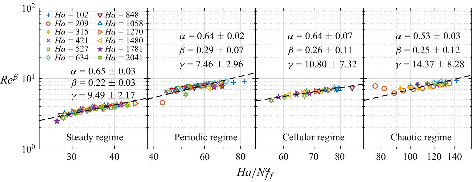
The dependence of  $Re(Ha,Ra,Pr)$ can also be given by
 \begin{equation} Re^{\beta} = \gamma \frac{Ha}{N_{ff}^{\alpha}}. \end{equation}
Similar to the normalization process of  $Nu$ depicted in figure 18, the results for
 $Re$ for the four flow regimes are shown in figure 20. Here
 $Re$ exhibits a consistent
 $\alpha$ value across all flow regimes except for the chaotic regime, where it converges to approximately 2/3. The parameter
 $\beta$ tends to approximate 1/4 across all flow regimes. Therefore, an empirical scaling relationship can be established as follows:
 \begin{equation} Re \sim (Ha^{{-}1}RaPr^{{-}1})^{4/3}. \end{equation}
Plot of  $Re^{\beta }$ vs
 $Ha/N_{ff}^{\alpha }$ for different flow regimes. The dashed lines are the best-fitted lines. The exponents
 $\alpha$ and
 $\beta$ for each regime are labelled.
At the end of this section we examine the impact of magnetic fields on heat and momentum transports compared with the cases without a magnetic field. The  $Nu$ and
 $Re$ are normalized by their respective values in the absence of a magnetic field, denoted as
 \begin{equation} Nu^{*}=\frac{Nu(Ra, Ha)-1}{Nu(Ra,0)-1} \end{equation}
and
 \begin{equation} Re^{*}=\frac{Re(Ra, Ha)}{Re(Ra,0)}. \end{equation}
We consider four Rayleigh numbers corresponding to distinct flow regimes. The outcomes are depicted in figure 21. Generally, the intensification of the magnetic field exerts a dampening effect on heat and momentum transport. The expected increase in heat transfer efficiency by up to 30 % with increasing  $Ha$, as previously noted (Vogt et al. Reference Vogt, Yang, Schindler and Eckert2021; Chen et al. Reference Chen, Wang and Ni2024a), is not observed in our experiment, which can be attributed to the different aspect ratios of the convection cell. In steady (figure 21a), periodic (figure 21b) and cellular regimes (figure 21c), changes in
 $Nu^{*}$ and
 $Re^{*}$ exhibit monotonic trends, signifying a coupled relationship in heat and momentum transports with respect to the results without a magnetic field within these flow regimes. Remarkably, the suppression of
 $Re^{*}$ by the magnetic field is more obvious, with its rate of decline surpassing that of
 $Nu^{*}$ as
 $Ha$ increases. The above results are similar to the results of Zürner et al. (Reference Zürner, Schindler, Vogt, Eckert and Schumacher2020) under the action of a vertical magnetic field. However, for the chaotic regime, the situation is different. Here, with a large
 $Ha$,
 $Re^{*}$ tends to increase while
 $Nu^{*}$ maintains a downward trend. This discrepancy might be due to the magnetic field suppressing the small-scale flow velocity component parallel to its direction while enhancing the large-scale flow velocity (Chen et al. Reference Chen, Wang and Ni2024a). Additionally, it can be observed that at small
 $Ha$, specifically in the range of
 $Ha = 102$ to 209,
 $Nu(Ra, Ha)$ closely resembles the Nusselt number without a magnetic field. This suggests that when
 $Ra$ is sufficiently large, a weaker magnetic field fails to significantly inhibit the bulk flow. Interestingly, at
 $Ha=102$,
 $Nu$ is even slightly enhanced by about 7 % compared with that in the absence of a magnetic field, possibly indicating that the weak magnetic field can enhance the coherence of the flow at high
 $Ra$ (Lim et al. Reference Lim, Chong, Ding and Xia2019). The decoupling behaviour of
 $Nu^*$ and
 $Re^*$ in the chaotic regime may be related to the trend of LSF gradually transforming from 3-D to Q2-D. The evidence, although not presented in the paper, indicates that when
 $Ra = 1.1 \times 10^7$ and
 $Ha = 102$, the time-averaged flow orientations at the top and bottom heights are
 $\langle \theta _{t} \rangle _{t}=131.28^{\circ }$ and
 $\langle \theta _{b} \rangle _{t}=127.58^{\circ }$, respectively, indicating that the convection plane is located along the diagonal of the cell. However, when
 $Ra = 1.1 \times 10^7$ and
 $Ha = 634$, the time-averaged flow orientations at the top and bottom heights are
 $\langle \theta _{t} \rangle _{t}=94.35^{\circ }$ and
 $\langle \theta _{b} \rangle _{t}=99.07^{\circ }$, suggesting that the convection plane is near the central plane of the cell, similar to the cases in the steady regime.
Normalized  $Nu$ and
 $Re$ over
 $Ha$ for four selected
 $Ra$. Each
 $Ra$ corresponds to a flow regime: (a) steady regime, (b) periodic regime, (c) cellular regime and (d) chaotic regime. The dashed lines indicated the value of 1.

6. Conclusions
This paper presents a systematic experimental study of liquid metal thermal convection in a cuboid cell with  $\varGamma \approx 0.5$ under a horizontal magnetic field. Liquid metal GaInSn was selected as the working fluid, covering a Rayleigh number range of
 $3.8\times 10^5$ to
 $1.1\times 10^7$ while the Prandtl number was fixed at 0.029. The magnetic field strength ranged from 0 to 0.5 T, corresponding to a Hartmann number range of
 $0 \leqslant Ha \leqslant 2041$.
Utilizing a combination of the multi-thermal-probe method and a homemade MPUDV, we reconstructed the flow structure in a larger ( $Ra, Ha$) parameter space. Five flow regimes were identified based on the discovered flow structures, with critical transition curves defined between them. A novel flow morphology featuring four multi-roll structures that interact with each other was observed over a wide parameter range. Multiple vortices undergo a process where diagonal vortices are initially compressed, before gradually expanding again. Then, the four vortices will be comparable in size, and eventually, the two diagonal vortices will become larger and squeeze another pair of diagonal vortices. This dynamic process undergoes periodic changes over time, leading to velocity reversals near the upper and lower boundaries of the cell. The flow morphology arises from the transfer of Fourier mode energy from the first order to higher orders. To the best of our knowledge, this flow morphology represents the first experimental discovery of thermal convection under the influence of a horizontal magnetic field.
We investigated the flow characteristics of each flow regime. Among these regimes, the presence of the double-roll structure resulted in a low azimuthal temperature difference region at the middle height of the cell in the periodic regime. This phenomenon coincided with an increase in temperature differences between the upper and lower parts of the system, consequently leading to an escalation in the wall temperature gradient. The least-squares fitting of the data revealed scaling relationships between wall temperature gradient and combinations of  $Ra, Ha$ and
 $Pr$ in each flow regime. The unified scaling laws of temperature gradient suggest that a common mechanism operates within each regime. Furthermore, the electromagnetic force (Lorentz force) or buoyancy force yields distinct effects on flow oscillation. The fitted scaling laws of the oscillation frequencies reveal that the electromagnetic force works to suppress oscillation frequency, while the buoyancy force tends to elevate it. However, changes in magnetic field or buoyancy do not alter the global temperature oscillation amplitude.
Distinct heat and momentum transport efficiencies were observed across different flow regimes. The distributions of heat and momentum transport varied significantly between different flow regimes. As the Rayleigh number increases in the steady regime, heat and momentum transport approach levels similar to those observed in the absence of a magnetic field. However, periodic and cellular regimes showed different behaviours, with the periodic regime causing a significant decrease in heat transfer. Compared with the reduction in heat transfer caused by the double-roll structure in water (Sun, Xi & Xia Reference Sun, Xi and Xia2005; Xi & Xia Reference Xi and Xia2008; Weiss & Ahlers Reference Weiss and Ahlers2011), the influence of the double-roll structure in liquid metal under the influence of a horizontal magnetic field is even more pronounced on heat transfer. Extrapolating from steady regime data suggested a potential heat transfer decrease of up to 36 % when the flow transitions to the periodic regime.
Finally, through extensive data fitting, we obtained empirical scaling relationships of  $Nu(Ha, Ra, Pr)$ and
 $Re(Ha, Ra, Pr)$ applicable across a wide range, i.e.
 $Nu \sim (Ha^{-2/3}RaPr^{-1})^{3/5}$ and
 $Re \sim (Ha^{-1}RaPr^{-1})^{4/3}$. To the best of our knowledge, few studies exist on the scaling laws of heat and momentum transport under horizontal magnetic fields. However, extensive research has been conducted on global transport scaling laws under the influence of vertical magnetic fields already mentioned in § 1. The empirical scaling relationships obtained in our experiment pose open questions for further investigation. Our convection cell, being an elongated square cavity, differs significantly from the cylinder with perfect symmetry, which introduces potential wells at the four corners of the cell (Ji & Brown Reference Ji and Brown2020), altering the flow pattern. Additionally, the small
 $\varGamma$ imposes strong geometric constraints influencing global transport (Ahlers et al. Reference Ahlers2022). Weaker magnetic fields and narrower ranges of
 $Ra$ further compound the complexity of the flow. These factors mentioned above all lead to difficulties in the theoretical derivation of global transport scalings under the action of horizontal magnetic fields.
In conclusion, our work provides systematic and significant insights into the flow morphologies and global transport properties of liquid metal thermal convection under a horizontal magnetic field. However, we acknowledge the limitations of our work, and investigations of magnetohydrodynamic convection in liquid metals would be desirable for future research.
Funding
The authors gratefully acknowledge support from the National Key Research and Development Program of China (no. 2022YFE03130000), NSFC (nos. 51927812, 52176086, 52222607) and the Young Talent Support Plan of Xi'an Jiaotong University.
Declaration of interests
The authors report no conflict of interest.



