1 Introduction
Turbulence-driven relative motion of high-inertia particles is relevant in astrophysical scenarios, such as the interstellar medium, protoplanetary disks and the atmospheres of planets and dwarf stars (Chiang & Youdin Reference Chiang and Youdin2005; Pan et al.
Reference Pan, Padoan, Scalo, Kritsuk and Norman2011). Specifically, the ‘sticking’ of dust particles in protoplanetary disks is believed to be the mechanism for planetesimal formation. An intriguing question that the astrophysicists are investigating concerns the effects of turbulence on the dispersion, sedimentation, collisional coalescence and fragmentation of dust grains. The viscous relaxation times,
 $\unicode[STIX]{x1D70F}_{v}$
, of these particles are significantly large, with estimated
 $St_{\unicode[STIX]{x1D702}}\sim 10{-}100$
(Pan et al.
Reference Pan, Padoan, Scalo, Kritsuk and Norman2011), where
 $St_{\unicode[STIX]{x1D702}}=\unicode[STIX]{x1D70F}_{v}/\unicode[STIX]{x1D70F}_{\unicode[STIX]{x1D702}}$
is the Stokes number based on the Kolmogorov time scale
 $\unicode[STIX]{x1D70F}_{\unicode[STIX]{x1D702}}$
.
The two principal quantities describing the relative motion of inertial particles in a turbulent flow are: (i) the radial distribution function (RDF), which is a measure of the particle spatial clustering, and (ii) the probability density function (PDF) of pair relative velocities, which quantifies the particle encounter rate. The RDF and the relative-velocity PDF are both key inputs to the particle collision kernel, and depend sensitively on the Stokes number. Both statistics can be determined through direct numerical simulations (DNS) of particle-laden turbulent flows. However, DNS suffers from the well-known computational limitation on the Reynolds numbers that can be achieved. This drawback of DNS is one of the motivating factors for developing PDF equation-based stochastic models for particle-laden turbulent flows.
Recently, we developed a stochastic theory for the relative velocities and positions of high-inertia monodisperse pairs in forced isotropic turbulence (Rani, Dhariwal & Koch Reference Rani, Dhariwal and Koch2014). The theory involved deriving a closure for the diffusivity tensor characterizing the relative-velocity-space diffusion current in the PDF kinetic equation of particle-pair separation and relative velocity. Since we had considered the
 $St_{r}\gg 1$
limit, the pair PDF equation is of the classical Fokker–Planck form (
 $St_{r}$
is the Stokes number based on the time scale
 $\unicode[STIX]{x1D70F}_{r}$
of eddies whose size is of the order of pair separation
 $r$
). Using the diffusivity formulation, one can perform Langevin simulations of pair relative velocities and positions, which is equivalent to simulating the Fokker–Planck equation.
In this context, the current study has two main objectives. First, we perform a quantitative analysis of the three forms of the diffusivity derived in Rani et al. (Reference Rani, Dhariwal and Koch2014). The insights gained will help us understand the implications of the approximations made in deriving the diffusivities, as well as guide future improvements to the theory. In the
 $St_{r}\gg 1$
limit, we perform a comparative analysis of the current and (Zaichik & Alipchenkov Reference Zaichik and Alipchenkov2003) diffusivity closures, as well as the predictions of relative-motion statistics by the two theories. The second objective is to compute the relative-motion statistics of particle pairs using both DNS and Langevin simulations (LS), and compare the corresponding results. The parametric inputs to the LS runs such as the Taylor micro-scale Reynolds number, dissipation rate, Kolmogorov scales, integral length scale and the root mean square (r.m.s.) fluctuating velocity were all obtained from DNS. Further, the energy spectrum needed to compute the analytical diffusivities is modelled such that it closely matches the DNS spectrum. Thus, the DNS and LS results are compared under conditions where a broad set of flow parameters, and not just
 $Re_{\unicode[STIX]{x1D706}}$
, is matched. Such a comparison will enable us to quantify the theory’s predictive abilities for pair dynamics in isotropic turbulence.
Zaichik & Alipchenkov (Reference Zaichik and Alipchenkov2003) developed a stochastic model for particle pairs that was conceived to be applicable for all Stokes numbers, provided that the Stokes drag force is applicable and is the dominant force acting on the particles. Although Rani et al. (Reference Rani, Dhariwal and Koch2014) and Zaichik & Alipchenkov (Reference Zaichik and Alipchenkov2003) are both based on a kinetic equation description of pair interactions, there are important fundamental distinctions between the two studies. The principal difference lies in the approach adopted to close the diffusion current in the PDF equation. Zaichik & Alipchenkov closed the diffusion current by using the Furutsu–Novikov–Donsker (FND) formula. The FND formula relates the diffusion current to a series expansion in the cumulants of the fluid relative velocities seen by the pairs (
 $\unicode[STIX]{x0394}\boldsymbol{u}$
) and the functional derivatives of the PDF with respect to
 $\unicode[STIX]{x0394}\boldsymbol{u}$
(Bragg & Collins Reference Bragg and Collins2014a
). They further assumed that
 $\unicode[STIX]{x0394}\boldsymbol{u}$
had a Gaussian distribution, for which the series expansion exactly reduces to only the second-order cumulant of
 $\unicode[STIX]{x0394}\boldsymbol{u}$
(Bragg & Collins Reference Bragg and Collins2014a
). In contrast, Rani et al. (Reference Rani, Dhariwal and Koch2014) developed a closure for the diffusion current based on a perturbation analysis of the pair PDF equation in the limit of high Stokes number. Another important difference concerns the simulation approach used in the two studies. Zaichik & Alipchenkov (Reference Zaichik and Alipchenkov2003) computed the statistics of pair separation and relative velocity by solving the equations for the zeroth, first and second relative-velocity moments of the master PDF equation. Rani et al. simulated the Langevin equations to evolve the relative velocities and positions of a large number of particle pairs. When compared to solving a finite number of moments equations, the Langevin approach is higher-order accurate in the sense that the LS inherently include all moments of the pair PDF. Another advantage of the LS approach is that it allows us to explicitly compute the PDFs of pair relative velocity at various separations, enabling us to track the transition in the nature of the PDF as the separations are reduced from the order of integral scale to that of Kolmogorov scale.
Bragg & Collins (Reference Bragg and Collins2014a
) performed a first-principles-based comparison of the Chun et al. (Reference Chun, Koch, Rani, Ahluwalia and Collins2005) and Zaichik & Alipchenkov (Reference Zaichik and Alipchenkov2007, Reference Zaichik and Alipchenkov2009) stochastic models for inertial pair dynamics in isotropic turbulence. The focus of that paper was to compare and analyse the predictions of particle clustering at sub-Kolmogorov-scale separations by the two theories. In the limit of
 $St_{\unicode[STIX]{x1D702}}\ll 1$
, Chun et al. (Reference Chun, Koch, Rani, Ahluwalia and Collins2005) developed closures for the drift and diffusion fluxes in the PDF equation for pair separation, where
 $St_{\unicode[STIX]{x1D702}}$
is the Stokes number based on the Kolmogorov time scale
 $\unicode[STIX]{x1D70F}_{\unicode[STIX]{x1D702}}$
. Using these closures, they derived a power-law expression for the RDF at sub-Kolmogorov separations, which showed good agreement with the DNS results. The Zaichik & Alipchenkov (Reference Zaichik and Alipchenkov2007) study improved upon their earlier study (Zaichik & Alipchenkov Reference Zaichik and Alipchenkov2003) by accounting for the unequal Lagrangian correlation time scales of the strain-rate and rotation-rate tensors. Bragg & Collins showed that the power-law exponents in the RDFs predicted by the two theories were in good agreement for
 $St_{\unicode[STIX]{x1D702}}\ll 1$
. They elaborated that this agreement was because the drift velocity predicted by Chun et al. was the same as the leading-order term in the drift velocity of Zaichik & Alipchenkov (Reference Zaichik and Alipchenkov2007). As is to be expected, for
 $St_{\unicode[STIX]{x1D702}}\sim 1$
, the theories diverge. Bragg & Collins also showed that the clustering of
 $St_{\unicode[STIX]{x1D702}}\ll 1$
particles was mainly due to the centrifuging process, whereas that of
 $St_{\unicode[STIX]{x1D702}}\sim 1$
particles was due to their path-history interactions with the turbulence.
In an accompanying study, Bragg & Collins (Reference Bragg and Collins2014b
) analysed the theories of Zaichik & Alipchenkov (Reference Zaichik and Alipchenkov2009), Pan & Padoan (Reference Pan and Padoan2010) and Gustavsson & Mehlig (Reference Gustavsson and Mehlig2011) by focusing on the second-order structure function of pair relative velocities,
 $\unicode[STIX]{x1D61A}_{2}^{\,p}(\boldsymbol{r},t)$
, predicted by these theories, where
 $\boldsymbol{r}$
is the separation vector. Formulation of
 $\unicode[STIX]{x1D61A}_{2}^{\,p}(\boldsymbol{r},t)$
is required to solve the governing equations for the moments of the pair PDF (Zaichik & Alipchenkov Reference Zaichik and Alipchenkov2009). One may also compute the variances of the pair relative velocity and its components longitudinal and transverse to
 $\boldsymbol{r}$
–
 $\langle U^{2}\rangle$
,
 $\langle U_{r}^{2}\rangle$
and
 $\langle U_{t}^{2}\rangle$
respectively – using
 $\unicode[STIX]{x1D61A}_{2}^{\,p}(\boldsymbol{r},t)$
(Pan & Padoan Reference Pan and Padoan2010). By comparing the predictions (primarily of the first two theories) with the DNS computed
 $\unicode[STIX]{x1D61A}_{2}^{\,p}(\boldsymbol{r},t)$
, Bragg & Collins (Reference Bragg and Collins2014b
) identified possible discrepancies in the theories. In the case of Gustavsson & Mehlig (Reference Gustavsson and Mehlig2011) theory, only qualitative insights could be drawn regarding its predictions of the structure function and the RDF, since some coefficients were left unspecified in their theory.
Ireland, Bragg & Collins (Reference Ireland, Bragg and Collins2015) performed an extensive parametric study of the effects of Reynolds number on inertial particle statistics through DNS of forced isotropic turbulence. They considered a wide range of Taylor micro-scale Reynolds numbers (
 $88\leqslant Re_{\unicode[STIX]{x1D706}}\leqslant 597$
), and computed the statistics of single particles, as well as pairs for Stokes numbers
 $0.05\leqslant St_{\unicode[STIX]{x1D702}}\leqslant 30$
. It was observed that for
 $St_{\unicode[STIX]{x1D702}}\lesssim 1$
, the RDF is essentially independent of
 $Re_{\unicode[STIX]{x1D706}}$
, whereas for
 $St_{\unicode[STIX]{x1D702}}\geqslant 10$
, the RDF increased with
 $Re_{\unicode[STIX]{x1D706}}$
at nearly all separations. The latter trend is captured by our theory as well. As identified in Bragg & Collins (Reference Bragg and Collins2014a
), the effects of preferential concentration on pair relative-velocity statistics were important for
 $St_{\unicode[STIX]{x1D702}}\lesssim 0.1$
, while the non-local effects due to particle sampling of turbulence become important for
 $St_{\unicode[STIX]{x1D702}}\gtrsim 0.2$
. The relative-velocity statistics of the
 $St_{\unicode[STIX]{x1D702}}\geqslant 10$
particles were found to increase strongly with
 $Re_{\unicode[STIX]{x1D706}}$
because these particles retain for long times the effects of their interactions with the inertial- and integral-scale eddies.
Some of the most detailed theoretical and computational studies of high
 $St_{\unicode[STIX]{x1D702}}$
particles were undertaken by Pan, Padoan and coworkers (Pan & Padoan Reference Pan and Padoan2010; Pan et al.
Reference Pan, Padoan, Scalo, Kritsuk and Norman2011; Pan & Padoan Reference Pan and Padoan2013, Reference Pan and Padoan2014a
,Reference Pan and Padoan
b
,Reference Pan and Padoan
c
, Reference Pan and Padoan2015). Pan & Padoan (Reference Pan and Padoan2010) derived an analytical model for the relative-velocity variance of inertial particles that is conceptually generalized across the entire range of particle Stokes numbers (this study will be hereafter referred to as PP10). The PP10 model is based on expressing the pair relative-velocity structure function
 $\unicode[STIX]{x1D61A}_{2}^{\,p}(\boldsymbol{r},t)$
in terms of the fluid relative-velocity structure function
 $\unicode[STIX]{x1D61A}_{2}^{\,f}(\boldsymbol{r},t)$
, where
 $\unicode[STIX]{x1D61A}_{2}^{\,f}(\boldsymbol{r},t)$
is the Lagrangian correlation of fluid relative velocities along inertial particle-pair trajectories. Subsequently, they approximated
 $\unicode[STIX]{x1D61A}_{2}^{\,f}(\boldsymbol{r},t)$
as the product of the Eulerian structure tensor of turbulence and the Lagrangian autocorrelation of fluid relative velocities. Using this theory, they calculated the statistics of pair relative velocity (up to the second moment) for
 $1\leqslant St_{\unicode[STIX]{x1D702}}\leqslant 100$
, and compared these predictions with DNS data over a smaller Stokes number range
 $1\leqslant St_{\unicode[STIX]{x1D702}}\leqslant 10$
. Good agreement between the model and DNS results was obtained. However, PP10 is limited to modelling the lower-order moments of pair relative velocity, and does not provide any means to obtain the RDF, or the PDF of relative velocities.
Pan et al. (Reference Pan, Padoan, Scalo, Kritsuk and Norman2011) performed a DNS study of particle clustering in isotropic turbulence for
 $1\lesssim St_{\unicode[STIX]{x1D702}}\lesssim 100$
. In agreement with prior DNS and theoretical studies (e.g. Chun et al.
Reference Chun, Koch, Rani, Ahluwalia and Collins2005), they observed that the RDF shows a power-law scaling for pair separations in the dissipative range, with the exponent being a function of Stokes number. Further, particles whose response times scale with inertial-range time scales show clustering at inertial separations, which is manifested as the peaking of RDF for these separations and subsequent plateauing for smaller separations. As seen in Chun et al. (Reference Chun, Koch, Rani, Ahluwalia and Collins2005), the RDF of bidisperse pairs becomes flat at small scales, confirming that such pairs show weaker clustering than monodisperse ones.
Perhaps the broadest range of Stokes numbers considered thus far in particle-laden isotropic turbulence is by Pan & Padoan (Reference Pan and Padoan2013). In that study, relative-velocity statistics of
 $0.1\leqslant St_{\unicode[STIX]{x1D702}}\leqslant 800$
particles were computed using both DNS and the model of PP10 (Pan & Padoan Reference Pan and Padoan2010). Their goal was to investigate the relative-motion statistics for separations smaller than the Kolmogorov scale, so as to draw insights on the collision rates of dust particles in protoplanetary disks. In protoplanetary turbulence, dust particles are much smaller than the Kolmogorov length scale (
 $\unicode[STIX]{x1D702}\sim 1$
km). Therefore, they focused on understanding and quantifying pair relative motion for separations
 $r\rightarrow 0$
. Since such a fine resolution of separations is computationally prohibitive, Pan & Padoan (Reference Pan and Padoan2013) computed relative-velocity statistics for separations as small as
 $0.25\unicode[STIX]{x1D702}$
, and then extrapolated these insights to smaller
 $r$
. The extrapolation involved grouping the pairs into two categories: continuous and caustic types. Continuous-type pairs are those that may have started their journey as uncorrelated particles with high relative velocities at large separations, but decelerate as their separations decrease and remain correlated far longer than the flow time scales that influence their relative motion. Caustic-type pairs are those that remain uncorrelated with large relative velocities throughout their flight. It is believed that caustic pairs may significantly enhance collision rates, and that they dominate collision rates as
 $r\rightarrow 0$
. Predictions using PP10 of relative velocity and its components parallel and transverse to the separation vector showed good agreement with their DNS data.
Under the limits
 $St_{r}\gg 1$
and
 $St_{I}\gg 1$
, Rani et al. (Reference Rani, Dhariwal and Koch2014) derived the transport equation for the PDF
 $\unicode[STIX]{x1D6FA}(\boldsymbol{r},\boldsymbol{U})$
of pair separation (
 $\boldsymbol{r}$
) and relative velocity (
 $\boldsymbol{U}$
). Here, the Stokes number
 $St_{r}$
is based on the time scale
 $\unicode[STIX]{x1D70F}_{r}$
of eddies whose size scales with separation
 $r$
, and
 $St_{I}$
is based on the integral time scale
 $\unicode[STIX]{x1D70F}_{I}$
. The transport equation for
 $\unicode[STIX]{x1D6FA}(\boldsymbol{r},\boldsymbol{U})$
, which is of the Fokker–Planck type, contains a diffusivity tensor in the
 $\boldsymbol{U}$
space. We showed that the diffusivity is equal to
 $1/\unicode[STIX]{x1D70F}_{v}^{2}$
times the time integral of the Eulerian two-time correlation of fluid relative velocities seen by nearly stationary pairs (
 $\unicode[STIX]{x1D70F}_{v}$
is the particle viscous relaxation time). In the current study, the two-time correlation is directly computed using DNS of forced isotropic turbulence containing stationary particles. The DNS-computed correlation when integrated in time yields what we will refer to as the first closure form of diffusivity (CF1). An advantage of the CF1 diffusivity is that it will provide us a means to assess the diffusivity formulation of Zaichik, Simonin & Alipchenkov (Reference Zaichik, Simonin and Alipchenkov2003), Zaichik & Alipchenkov (Reference Zaichik and Alipchenkov2007) in the
 $St_{r}\gg 1$
limit.
Alternatively to CF1, the Eulerian two-time correlation may be resolved analytically through the approximation that the temporal change in the fluid relative velocities seen by a pair is primarily due to the advection of size
 $r$
eddies past the pair by larger eddies. Based on this physical picture and through an analogy with the Taylor hypothesis, one may transform the two-time correlation into two-point correlations of fluid velocities, allowing us to analytically formulate the diffusivity in terms of the energy spectrum. Rani et al. (Reference Rani, Dhariwal and Koch2014) derived two expressions based on whether the pair centre of mass was held fixed or allowed to move during integral time scales, the latter being an improvement over the former at finite
 $St_{I}$
. We will refer to these expressions as the second and third closure forms of diffusivity (CF2 and CF3), respectively.
In the current study, we first undertake a detailed analysis of the three closure forms of the diffusivity. Such an analysis will provide quantitative insights into the effects of the approximations entailed in deriving the closures, i.e. that the pairs are essentially fixed, and that the Eulerian two-time correlation may be expressed in terms of two-point correlations. Second, we perform both Langevin and direct numerical simulations to compute a number of statistics quantifying pair relative motion. Three sets of Langevin simulations are performed, corresponding to the three diffusivity forms. The LS results are compared with each other and with the DNS data. To our knowledge, this study presents the first comparison of the stochastic and DNS predictions of the relative-velocity PDFs at separations spanning the entire range of turbulent scales. The pair statistics from LS are compared with those from DNS of particle-laden isotropic turbulence for
 $St_{\unicode[STIX]{x1D702}}=10,20,40,80$
and
 $Re_{\unicode[STIX]{x1D706}}=76,131$
. Statistics such as the RDF, relative-velocity moments and PDFs, and the collision kernel are compared. Furthermore, we compare the present results with those from Zaichik et al. (Reference Zaichik, Simonin and Alipchenkov2003), Zaichik & Alipchenkov (Reference Zaichik and Alipchenkov2009) where available.
The organization of the paper is as follows: § 2 presents the important details of the closure theory, as well as identifies the three closure forms that are analysed in this study. Section 3 discusses the computational details of the direct numerical and Langevin simulations. Section 4 presents an analysis of the diffusivity forms, as well as a comparison of the pair relative-motion statistics obtained from LS and DNS. We conclude by summarizing our findings in § 5.
2 Theory
We begin with an overview of the Rani et al. (Reference Rani, Dhariwal and Koch2014) stochastic model for particle pairs in the limit of high Stokes number. A review of the theory will provide the necessary background for the subsequent discussion of the three closure forms that are investigated in this study.
Rani et al. (Reference Rani, Dhariwal and Koch2014) considered the pair phase-space density (PSD)
 $P(\boldsymbol{r},\boldsymbol{U},\boldsymbol{x},\boldsymbol{V};t)$
, which is the PSD of a particle pair with separation
 $\boldsymbol{r}$
, relative velocity
 $\boldsymbol{U}$
, and centre-of-mass position and velocity
 $\boldsymbol{x}$
and
 $\boldsymbol{V}$
, respectively. The inclusion of
 $\boldsymbol{x}$
and
 $\boldsymbol{V}$
in the state vector was motivated by the physical scenario that the dynamics of pair centre of mass can influence the way a pair samples turbulence. Conservation of PSD
 $P$
yields
 $$\begin{eqnarray}\displaystyle \frac{\unicode[STIX]{x2202}P}{\unicode[STIX]{x2202}t}+\unicode[STIX]{x1D735}_{\boldsymbol{r}}\boldsymbol{\cdot }(\boldsymbol{U}P)+\unicode[STIX]{x1D735}_{\boldsymbol{U}}\boldsymbol{\cdot }(\dot{\boldsymbol{U}}P)+\unicode[STIX]{x1D735}_{\boldsymbol{x}}\boldsymbol{\cdot }(\boldsymbol{V}P)+\unicode[STIX]{x1D735}_{\boldsymbol{V}}\boldsymbol{\cdot }(\dot{\boldsymbol{V}}P)=0, & & \displaystyle\end{eqnarray}$$
where
 $\unicode[STIX]{x1D735}_{\boldsymbol{r}}$
,
 $\unicode[STIX]{x1D735}_{\boldsymbol{x}}$
,
 $\unicode[STIX]{x1D735}_{\boldsymbol{U}}$
, and
 $\unicode[STIX]{x1D735}_{\boldsymbol{V}}$
denote gradients with respect to the corresponding state variables.
Assuming Stokes drag law to be valid, the governing equations for monodisperse pairs are:
 $$\begin{eqnarray}\displaystyle & \displaystyle \frac{\text{d}\boldsymbol{U}}{\text{d}t}=-\frac{1}{\unicode[STIX]{x1D70F}_{v}}[\boldsymbol{U}(t)-\unicode[STIX]{x0394}\boldsymbol{u}(\boldsymbol{r},\boldsymbol{x},t)] & \displaystyle\end{eqnarray}$$
 $$\begin{eqnarray}\displaystyle & \displaystyle \frac{\text{d}\boldsymbol{V}}{\text{d}t}=-\frac{1}{\unicode[STIX]{x1D70F}_{v}}\left[\boldsymbol{V}(t)-\frac{\boldsymbol{u}(\boldsymbol{R}_{1}(t),t)+\boldsymbol{u}(\boldsymbol{R}_{2}(t),t)}{2}\right]=-\frac{1}{\unicode[STIX]{x1D70F}_{v}}[\boldsymbol{V}(t)-\boldsymbol{u}_{cm}(\boldsymbol{R}_{1}(t),\boldsymbol{R}_{2}(t),t)],\qquad & \displaystyle\end{eqnarray}$$
 $\unicode[STIX]{x1D70F}_{v}$
is the particle response time,
 $\boldsymbol{R}_{1}(t)$
and
 $\boldsymbol{R}_{2}(t)$
are the particle positions at time
 $t$
,
 $\unicode[STIX]{x0394}\boldsymbol{u}(\boldsymbol{r},\boldsymbol{x},t)=[\boldsymbol{u}(\boldsymbol{R}_{2}(t),t)-\boldsymbol{u}(\boldsymbol{R}_{1}(t),t)]$
is the seen fluid relative velocity and
 $\boldsymbol{u}_{cm}(\boldsymbol{R}_{1}(t),\boldsymbol{R}_{2}(t),t)=[\boldsymbol{u}(\boldsymbol{R}_{1}(t),t)+\boldsymbol{u}(\boldsymbol{R}_{2}(t),t)]/2$
. The velocity
 $\boldsymbol{u}_{cm}$
can be determined from
 $\boldsymbol{x}$
and
 $\boldsymbol{r}$
since
 $\boldsymbol{R}_{1}=\boldsymbol{x}-(\boldsymbol{r}/2)$
and
 $\boldsymbol{R}_{2}=\boldsymbol{x}+(\boldsymbol{r}/2)$
.
Substitution of the pair governing equations into (A 9) followed by ensemble averaging over flow realizations gives the equation for the PDF
 $\langle P\rangle$
:
 $$\begin{eqnarray}\displaystyle & & \displaystyle \frac{\unicode[STIX]{x2202}\langle P\rangle }{\unicode[STIX]{x2202}t}+\unicode[STIX]{x1D735}_{\boldsymbol{r}}\boldsymbol{\cdot }(\boldsymbol{U}\langle P\rangle )+\unicode[STIX]{x1D735}_{\boldsymbol{x}}\boldsymbol{\cdot }(\boldsymbol{V}\langle P\rangle )-\frac{1}{\unicode[STIX]{x1D70F}_{v}}\unicode[STIX]{x1D735}_{\boldsymbol{U}}\boldsymbol{\cdot }(\boldsymbol{U}\langle P\rangle )-\frac{1}{\unicode[STIX]{x1D70F}_{v}}\unicode[STIX]{x1D735}_{\boldsymbol{V}}\boldsymbol{\cdot }(\boldsymbol{V}\langle P\rangle )\nonumber\\ \displaystyle & & \displaystyle \quad +\,\frac{1}{\unicode[STIX]{x1D70F}_{v}}\unicode[STIX]{x1D735}_{\boldsymbol{U}}\boldsymbol{\cdot }\langle \unicode[STIX]{x0394}\boldsymbol{u}P\rangle +\frac{1}{\unicode[STIX]{x1D70F}_{v}}\unicode[STIX]{x1D735}_{\boldsymbol{V}}\boldsymbol{\cdot }\langle \boldsymbol{u}_{cm}P\rangle =0,\end{eqnarray}$$
where
 $\langle \cdot \rangle$
denotes ensemble averaging, and the terms
 $\langle \unicode[STIX]{x0394}\boldsymbol{u}P\rangle$
and
 $\langle \boldsymbol{u}_{cm}P\rangle$
require closure. These terms represent turbulence–pair interactions and turbulence–centre of mass interactions, respectively. In the limit of high Stokes number, they can be expressed as Fokker–Planck-type diffusion terms in the phase space.
Using the decomposition
 $P=\langle P\rangle +P^{\prime }$
, we can write
 $\langle \unicode[STIX]{x0394}\boldsymbol{u}P\rangle =\langle \unicode[STIX]{x0394}\boldsymbol{u}P^{\prime }\rangle$
and
 $\langle \boldsymbol{u}_{cm}P\rangle =\langle \boldsymbol{u}_{cm}P^{\prime }\rangle$
, since
 $\langle \unicode[STIX]{x0394}\boldsymbol{u}\rangle =0$
and
 $\langle u_{cm}\rangle =0$
in isotropic turbulence. This suggests that one may derive closures for these terms by solving for
 $P^{\prime }$
in terms of
 $\langle P\rangle$
. Substituting
 $P=\langle P\rangle +P^{\prime }$
into (A 9) and subtracting (A 10), the governing equation for
 $P^{\prime }$
can be obtained as:
 $$\begin{eqnarray}\displaystyle & & \displaystyle \frac{\unicode[STIX]{x2202}P^{\prime }}{\unicode[STIX]{x2202}t}+\unicode[STIX]{x1D735}_{\boldsymbol{r}}\boldsymbol{\cdot }(\boldsymbol{U}P^{\prime })+\unicode[STIX]{x1D735}_{\boldsymbol{ x}}\boldsymbol{\cdot }(\boldsymbol{V}P^{\prime })-\frac{1}{St_{I}}\unicode[STIX]{x1D735}_{\boldsymbol{U}}\boldsymbol{\cdot }(\boldsymbol{U}P^{\prime })-\frac{1}{St_{I}}\unicode[STIX]{x1D735}_{\boldsymbol{V}}\boldsymbol{\cdot }(\boldsymbol{V}P^{\prime })\nonumber\\ \displaystyle & & \displaystyle \quad +\,\frac{1}{St_{I}}\unicode[STIX]{x1D735}_{\boldsymbol{U}}\boldsymbol{\cdot }(\unicode[STIX]{x0394}\boldsymbol{u}P^{\prime })+\frac{1}{St_{I}}\unicode[STIX]{x1D735}_{\boldsymbol{V}}\boldsymbol{\cdot }(\boldsymbol{u}_{cm}P^{\prime })=-\frac{1}{St_{I}}\unicode[STIX]{x1D735}_{\boldsymbol{U}}\boldsymbol{\cdot }(\unicode[STIX]{x0394}\boldsymbol{u}\langle P\rangle )\nonumber\\ \displaystyle & & \displaystyle \quad -\,\frac{1}{St_{I}}\unicode[STIX]{x1D735}_{\boldsymbol{V}}\boldsymbol{\cdot }(\boldsymbol{u}_{cm}\langle P\rangle )+\frac{1}{St_{I}}\unicode[STIX]{x1D735}_{\boldsymbol{U}}\boldsymbol{\cdot }\langle \unicode[STIX]{x0394}\boldsymbol{u}P^{\prime }\rangle +\frac{1}{St_{I}}\unicode[STIX]{x1D735}_{\boldsymbol{V}}\boldsymbol{\cdot }\langle \boldsymbol{u}_{cm}P^{\prime }\rangle ,\end{eqnarray}$$
where
 $St_{I}=\unicode[STIX]{x1D70F}_{v}/\unicode[STIX]{x1D70F}_{I}$
, and terms are made dimensionless using integral length scale (
 $L$
), integral time scale (
 $\unicode[STIX]{x1D70F}_{I}$
), and r.m.s. fluctuating velocity (
 $u_{rms}$
).
Recognizing that
 $P^{\prime }$
may be expressed as a perturbation expansion in
 $1/St_{I}$
(
 $St_{I}\gg 1$
), we can write to leading order
 $P^{\prime }=(1/St)P_{1}$
. Retaining
 $O(1/St_{I})$
terms in (2.5), we get
 $$\begin{eqnarray}\displaystyle \frac{\unicode[STIX]{x2202}P_{1}}{\unicode[STIX]{x2202}t}+\unicode[STIX]{x1D735}_{\boldsymbol{r}}\boldsymbol{\cdot }(\boldsymbol{U}P_{1})+\unicode[STIX]{x1D735}_{\boldsymbol{x}}\boldsymbol{\cdot }(\boldsymbol{V}P_{1})=-\unicode[STIX]{x1D735}_{\boldsymbol{U}}\boldsymbol{\cdot }(\unicode[STIX]{x0394}\boldsymbol{u}\langle P\rangle )-\unicode[STIX]{x1D735}_{\boldsymbol{V}}\boldsymbol{\cdot }(\boldsymbol{u}_{cm}\langle P\rangle ). & & \displaystyle\end{eqnarray}$$
Equation (2.6) is a Lagrangian evolution equation of
 $P_{1}$
in the
 $(\boldsymbol{r},\boldsymbol{x},t)$
space, with
 $\boldsymbol{U}$
and
 $\boldsymbol{V}$
held fixed.
In the limit of
 $St_{I}\gg 1$
and
 $St_{r}\gg 1$
, Rani et al. (Reference Rani, Dhariwal and Koch2014) showed that the two convective terms on the left-hand side of (2.6) can be neglected compared to
 $\unicode[STIX]{x2202}P_{1}/\unicode[STIX]{x2202}t$
. We can now solve for
 $P_{1}$
such that
 $\boldsymbol{r}$
and
 $\boldsymbol{x}$
remain fixed, giving us
 $$\begin{eqnarray}\displaystyle \langle \unicode[STIX]{x0394}\boldsymbol{u}P^{\prime }\rangle & = & \displaystyle -\frac{1}{St_{I}^{2}}\int _{-\infty }^{0}\,\text{d}t\{\langle \unicode[STIX]{x0394}\boldsymbol{u}(\boldsymbol{x},\boldsymbol{r},0)\unicode[STIX]{x0394}\boldsymbol{u}(\boldsymbol{x},\boldsymbol{r},t)\rangle \boldsymbol{\cdot }\unicode[STIX]{x1D735}_{\boldsymbol{U}}\langle P\rangle (t)\nonumber\\ \displaystyle & & \displaystyle +\,\langle \unicode[STIX]{x0394}\boldsymbol{u}(\boldsymbol{x},\boldsymbol{r},0)\boldsymbol{u}_{cm}(\boldsymbol{R}_{1}(0),\boldsymbol{R}_{2}(0),t)\rangle \boldsymbol{\cdot }\unicode[STIX]{x1D735}_{\boldsymbol{V}}\langle P\rangle (t)\}\end{eqnarray}$$
 $$\begin{eqnarray}\displaystyle \langle \boldsymbol{u}_{cm}P^{\prime }\rangle & = & \displaystyle -\frac{1}{St_{I}^{2}}\int _{-\infty }^{0}\,\text{d}t\{\langle \boldsymbol{u}_{cm}(\boldsymbol{R}_{1}(0),\boldsymbol{R}_{2}(0),0)\unicode[STIX]{x0394}\boldsymbol{u}(\boldsymbol{x},\boldsymbol{r},t)\rangle \boldsymbol{\cdot }\unicode[STIX]{x1D735}_{\boldsymbol{U}}\langle P\rangle (t)\nonumber\\ \displaystyle & & \displaystyle +\,\langle \boldsymbol{u}_{cm}(\boldsymbol{R}_{1}(0),\boldsymbol{R}_{2}(0),0)\boldsymbol{u}_{cm}(\boldsymbol{R}_{1}(0),\boldsymbol{R}_{2}(0),t)\rangle \boldsymbol{\cdot }\unicode[STIX]{x1D735}_{\boldsymbol{V}}\langle P\rangle (t)\},\end{eqnarray}$$
where
 $\boldsymbol{r}$
,
 $\boldsymbol{x}$
, particle positions
 $\boldsymbol{R}_{1}$
and
 $\boldsymbol{R}_{2}$
, and the PDF
 $\langle P\rangle$
undergo little change during flow time scales.
At this point, it is pertinent to discuss the similarities and differences between the above perturbation analysis, and the renormalized perturbation approach used in Reeks (Reference Reeks1992). Reeks (Reference Reeks1992) pioneered the application of the Lagrangian history direct interaction (LHDI) method of Kraichnan (Reference Kraichnan1977) to derive the PDF equation for particle position and velocity, as well as a closure for the phase-space diffusion current. The derivation of the closure using the LHDI method entailed a renormalized perturbation expansion, which is effectively an expansion with
 $1/St_{I}$
as the perturbation parameter. Appendix A presents a detailed comparison of the two perturbation methods.
The time integrals of the four correlations on the right-hand side of (2.7)–(2.8) are, respectively, the diffusivities
 $\unicode[STIX]{x1D60B}_{UU}$
,
 $\unicode[STIX]{x1D60B}_{UV}$
,
 $\unicode[STIX]{x1D60B}_{VU}$
, and
 $\unicode[STIX]{x1D60B}_{VV}$
. Here
 $\unicode[STIX]{x1D60B}_{UU}$
and
 $\unicode[STIX]{x1D60B}_{VV}$
are diffusivities in the
 $\boldsymbol{U}$
-space and
 $\boldsymbol{V}$
-space, respectively;
 $\unicode[STIX]{x1D60B}_{UV}$
and
 $\unicode[STIX]{x1D60B}_{VU}$
are cross-diffusivities. Equation (A 10) for the PDF
 $\langle P\rangle$
may now be written as:
 $$\begin{eqnarray}\displaystyle & & \displaystyle \frac{\unicode[STIX]{x2202}\langle P\rangle }{\unicode[STIX]{x2202}t}+\unicode[STIX]{x1D735}_{\boldsymbol{r}}\boldsymbol{\cdot }(\boldsymbol{U}\langle P\rangle )+\unicode[STIX]{x1D735}_{\boldsymbol{x}}\boldsymbol{\cdot }(\boldsymbol{V}\langle P\rangle )-\frac{1}{\unicode[STIX]{x1D70F}_{v}}\unicode[STIX]{x1D735}_{\boldsymbol{U}}\boldsymbol{\cdot }(\boldsymbol{U}\langle P\rangle )-\frac{1}{\unicode[STIX]{x1D70F}_{v}}\unicode[STIX]{x1D735}_{\boldsymbol{V}}\boldsymbol{\cdot }(\boldsymbol{V}\langle P\rangle )\nonumber\\ \displaystyle & & \displaystyle \quad -\,\unicode[STIX]{x1D735}_{\boldsymbol{U}}\boldsymbol{\cdot }(\unicode[STIX]{x1D60B}_{UU}\boldsymbol{\cdot }\unicode[STIX]{x1D735}_{\boldsymbol{U}}\langle P\rangle +\unicode[STIX]{x1D60B}_{UV}\boldsymbol{\cdot }\unicode[STIX]{x1D735}_{\boldsymbol{V}}\langle P\rangle )\nonumber\\ \displaystyle & & \displaystyle \quad -\,\unicode[STIX]{x1D735}_{\boldsymbol{V}}\boldsymbol{\cdot }(\unicode[STIX]{x1D60B}_{VU}\boldsymbol{\cdot }\unicode[STIX]{x1D735}_{\boldsymbol{U}}\langle P\rangle +\unicode[STIX]{x1D60B}_{VV}\boldsymbol{\cdot }\unicode[STIX]{x1D735}_{\boldsymbol{V}}\langle P\rangle )=0.\end{eqnarray}$$
2.1 Three closure forms for diffusivity
 $\unicode[STIX]{x1D60B}_{UU}$

Since our primary interest is in the statistics of pair relative motion, we will consider a more tractable, lower-dimensional PDF
 $\unicode[STIX]{x1D6FA}(\boldsymbol{r},\boldsymbol{U})=\int \langle P\rangle (\boldsymbol{r},\boldsymbol{U},\boldsymbol{x},\boldsymbol{V};t)\,\text{d}\boldsymbol{V}$
, where the dependence on
 $\boldsymbol{x}$
was dropped due to homogeneity. In Rani et al. (Reference Rani, Dhariwal and Koch2014), we showed that (2.9) yields the following equation (in dimensional form) for
 $\unicode[STIX]{x1D6FA}(\boldsymbol{r},\boldsymbol{U})$
:
 $$\begin{eqnarray}\displaystyle \frac{\unicode[STIX]{x2202}\unicode[STIX]{x1D6FA}}{\unicode[STIX]{x2202}t}+\unicode[STIX]{x1D735}_{\boldsymbol{r}}\boldsymbol{\cdot }(\boldsymbol{U}\unicode[STIX]{x1D6FA})-\frac{1}{\unicode[STIX]{x1D70F}_{v}}\unicode[STIX]{x1D735}_{\boldsymbol{U}}\boldsymbol{\cdot }(\boldsymbol{U}\unicode[STIX]{x1D6FA})-\unicode[STIX]{x1D735}_{\boldsymbol{U}}\boldsymbol{\cdot }(\unicode[STIX]{x1D60B}_{UU}\boldsymbol{\cdot }\unicode[STIX]{x1D735}_{\boldsymbol{U}}\unicode[STIX]{x1D6FA})=0, & & \displaystyle\end{eqnarray}$$
where
 $\unicode[STIX]{x1D70F}_{v}$
is the particle viscous relaxation time and
 $\boldsymbol{r}$
and
 $\boldsymbol{U}$
are the pair separation and relative velocity, respectively. The diffusivity
 $\unicode[STIX]{x1D60B}_{UU}$
is given by
 $$\begin{eqnarray}\displaystyle \unicode[STIX]{x1D60B}_{UU} & = & \displaystyle \frac{1}{\unicode[STIX]{x1D70F}_{v}^{2}}\int _{-\infty }^{0}\langle \unicode[STIX]{x0394}\boldsymbol{u}(\boldsymbol{r},\boldsymbol{x},0)\unicode[STIX]{x0394}\boldsymbol{u}(\boldsymbol{r},\boldsymbol{x},t)\rangle \,\text{d}t,\end{eqnarray}$$
where the integrand is the Eulerian two-time correlation of fluid relative velocities, with both pair separation
 $\boldsymbol{r}$
and centre-of-mass position
 $\boldsymbol{x}$
held fixed. This formulation of diffusivity is valid under the conditions
 $St_{r}\gg 1$
and
 $St_{I}\gg 1$
.
In this study,
 $\unicode[STIX]{x1D60B}_{UU}$
in (2.11) is resolved using three approaches, giving rise to three closure forms. In the first closure form (CF1), the two-time correlation in (2.11) is directly computed from DNS of forced isotropic turbulence with stationary particles, and integrated in time to yield
 $\unicode[STIX]{x1D60B}_{UU}$
. In the second closure form (CF2), the Eulerian two-time correlation of relative velocities is converted into two-point correlations of fluid velocities, allowing us to derive an expression in terms of an integral over the wavenumber. In the third closure form (CF3),
 $\boldsymbol{r}$
remains fixed during flow time scales, but
 $\boldsymbol{x}$
responds to integral-scale eddies, i.e.
 $\boldsymbol{x}$
changes during integral time scales. Thus, CF3 attempts to improve upon and extend CF2’s validity to
 $St_{I}\sim 1$
. The effects of CF3, however, are anticipated to be seen only at the lower end of the Stokes number range considered. At higher Stokes numbers, CF2 and CF3 should show very similar behaviour.
One may regard CF1 as the most accurate among the three closure forms since a DNS-based evaluation of the Eulerian two-time correlation would entail no further approximations. But, CF2 and CF3, the latter in spite of its improvements, contain approximations made to obtain analytical expressions for diffusivity. The differences between CF1 and CF2/CF3, and their implications for pair statistics are extensively analysed in this study.
In the following discussion, we present the salient features of the derivation of CF2 and CF3 (details are in Rani et al.
Reference Rani, Dhariwal and Koch2014). The computational details of the evaluation of
 $\unicode[STIX]{x1D60B}_{UU}$
for CF1 are discussed in § 3.1.
2.2 CF2 and CF3
In arriving at (2.11), Rani et al. (Reference Rani, Dhariwal and Koch2014) considered the limits
 $St_{r}\gg 1$
and
 $St_{I}\gg 1$
. In these Stokes number regimes, particles are nearly stationary so that the temporal change in
 $\unicode[STIX]{x0394}\boldsymbol{u}$
experienced by pairs is primarily due to the evolution of turbulent scales and not due to pair (relative) motion itself. Rani et al. (Reference Rani, Dhariwal and Koch2014) approximated the temporal evolution of
 $\unicode[STIX]{x0394}\boldsymbol{u}$
at two positions separated by
 $\boldsymbol{r}$
as arising due to the passive advection of eddies of size
 $r$
by larger, integral-scale eddies. Hence, one may replace the Eulerian two-time correlation in (2.11) by a correlation of relative velocities seen by two pairs with the same
 $\boldsymbol{r}$
, but with the centres of mass separated by
 $\boldsymbol{u}_{I}t$
, where
 $\boldsymbol{u}_{I}$
is the large-scale fluid velocity. This would give us closure form 2 (CF2) for
 $\unicode[STIX]{x1D60B}_{UU}$
:
 $$\begin{eqnarray}\displaystyle \unicode[STIX]{x1D60B}_{UU}^{[2]}=\frac{1}{\unicode[STIX]{x1D70F}_{v}^{2}}\int _{-\infty }^{0}\langle \unicode[STIX]{x0394}\boldsymbol{u}(\boldsymbol{x},\boldsymbol{r},0)\unicode[STIX]{x0394}\boldsymbol{u}(\boldsymbol{x}+\boldsymbol{u}_{I}t,\boldsymbol{r},0)\rangle \,\text{d}t. & & \displaystyle\end{eqnarray}$$
Relaxing the
 $St_{I}\gg 1$
criterion to
 $St_{I}\sim 1$
enables us to account for the change in centre-of-mass position due to interactions with eddies of time scales
 ${\sim}\unicode[STIX]{x1D70F}_{v}$
, the centre-of-mass response time. This is done by replacing
 $\boldsymbol{u}_{I}$
with the relative velocity
 $\boldsymbol{W}$
between the large-scale eddies and the centre of mass, yielding closure form 3 (CF3):
 $$\begin{eqnarray}\displaystyle \unicode[STIX]{x1D60B}_{UU}^{[3]}(\boldsymbol{r},W)=\frac{1}{\unicode[STIX]{x1D70F}_{v}^{2}}\int _{-\infty }^{0}\langle \unicode[STIX]{x0394}\boldsymbol{u}(\boldsymbol{x},\boldsymbol{r},t)\unicode[STIX]{x0394}\boldsymbol{u}(\boldsymbol{x}+\boldsymbol{W}t,\boldsymbol{r},t)\rangle \,\text{d}t. & & \displaystyle\end{eqnarray}$$
In the discussion that follows, we will focus on CF3, since the final expressions for CF2 and CF3 differ only by a constant factor.
The CF3 diffusivity can then be expressed as an average over all values of
 $\boldsymbol{W}$
as:
 $$\begin{eqnarray}\displaystyle \unicode[STIX]{x1D60B}_{UU}^{[3]}(\boldsymbol{r})=\int \unicode[STIX]{x1D60B}_{UU}^{[3]}(\boldsymbol{r},W)\unicode[STIX]{x1D6F7}(\boldsymbol{W})\,\text{d}\boldsymbol{W}, & & \displaystyle\end{eqnarray}$$
where
 $\unicode[STIX]{x1D6F7}(\boldsymbol{W})$
is the PDF of
 $\boldsymbol{W}$
, and
 $$\begin{eqnarray}\displaystyle & & \displaystyle \unicode[STIX]{x1D60B}_{UU}^{[3]}(\boldsymbol{r},W)=\frac{1}{\unicode[STIX]{x1D70F}_{v}^{2}}\int _{-\infty }^{0}\langle \unicode[STIX]{x0394}\boldsymbol{u}(\boldsymbol{x},\boldsymbol{r},t)\unicode[STIX]{x0394}\boldsymbol{u}(\boldsymbol{x}+\boldsymbol{W}t,\boldsymbol{r},t)\rangle \,\text{d}t\nonumber\\ \displaystyle & & \displaystyle \quad =\frac{1}{\unicode[STIX]{x1D70F}_{v}^{2}}\int _{-\infty }^{0}\left\langle \left[\boldsymbol{u}(\boldsymbol{x}+\frac{1}{2}\boldsymbol{r},t)-\boldsymbol{u}(\boldsymbol{x}-\frac{1}{2}\boldsymbol{r},t)\right]\right.\nonumber\\ \displaystyle & & \displaystyle \qquad \left.\times \left[\boldsymbol{u}(\boldsymbol{x}+\boldsymbol{W}t+\frac{1}{2}\boldsymbol{r},t)-\boldsymbol{u}(\boldsymbol{x}+\boldsymbol{W}t-\frac{1}{2}\boldsymbol{r},t)\right]\right\rangle \,\text{d}t\nonumber\\ \displaystyle & & \displaystyle \quad =\frac{1}{\unicode[STIX]{x1D70F}_{v}^{2}}\int _{-\infty }^{0}\left\langle \boldsymbol{u}(\boldsymbol{x}+\frac{1}{2}\boldsymbol{r},t)\boldsymbol{u}(\boldsymbol{x}+\boldsymbol{W}t+\frac{1}{2}\boldsymbol{r},t)-\boldsymbol{u}(\boldsymbol{x}+\frac{1}{2}\boldsymbol{r},t)\boldsymbol{u}(\boldsymbol{x}+\boldsymbol{W}t-\frac{1}{2}\boldsymbol{r},t)\right.\nonumber\\ \displaystyle & & \displaystyle \qquad \left.-\,\boldsymbol{u}(\boldsymbol{x}-\frac{1}{2}\boldsymbol{r},t)\boldsymbol{u}(\boldsymbol{x}+\boldsymbol{W}t+\frac{1}{2}\boldsymbol{r},t)+\boldsymbol{u}(\boldsymbol{x}-\frac{1}{2}\boldsymbol{r},t)\boldsymbol{u}(\boldsymbol{x}+\boldsymbol{W}t-\frac{1}{2}\boldsymbol{r},t)\right\rangle \,\text{d}t.\end{eqnarray}$$
Since
 $\boldsymbol{W}$
is principally influenced by the large-scale fluid eddies, its PDF can be considered as Gaussian (Batchelor Reference Batchelor1953):
 $$\begin{eqnarray}\displaystyle \unicode[STIX]{x1D6F7}(\boldsymbol{W})=\frac{1}{\sqrt{(2\unicode[STIX]{x03C0}W_{rms}^{2})^{3}}}\text{e}^{-(W^{2}/(2W_{rms}^{2}))}, & & \displaystyle\end{eqnarray}$$
where
 $W_{rms}$
is the r.m.s. fluctuating velocity of
 $\boldsymbol{W}$
. The two-point velocity correlations in (2.15) may be expressed in terms of the velocity spectrum tensor
 $\unicode[STIX]{x1D619}(\boldsymbol{k})$
, allowing us to further analytically resolve this equation.
For isotropic turbulence, we can write
 $\unicode[STIX]{x1D60B}_{UU}$
as:
 $$\begin{eqnarray}\displaystyle \unicode[STIX]{x1D60B}_{UU,ij}=\unicode[STIX]{x1D60B}_{UU,\bot }\left(\unicode[STIX]{x1D6FF}_{ij}-\frac{r_{i}r_{j}}{r^{2}}\right)+\unicode[STIX]{x1D60B}_{UU,||}\frac{r_{i}r_{j}}{r^{2}}. & & \displaystyle\end{eqnarray}$$
For CF3, Rani et al. (Reference Rani, Dhariwal and Koch2014) derived the following forms for
 $\unicode[STIX]{x1D60B}_{UU,\bot }$
and
 $\unicode[STIX]{x1D60B}_{UU,||}$
:
 $$\begin{eqnarray}\displaystyle & & \displaystyle \unicode[STIX]{x1D60B}_{UU,\bot }^{[3]}(r)=\frac{1}{2}\frac{2\unicode[STIX]{x03C0}^{2}}{\unicode[STIX]{x1D70F}_{v}^{2}}\sqrt{\frac{1}{(2\unicode[STIX]{x03C0})^{3}W_{rms}^{2}}}\nonumber\\ \displaystyle & & \displaystyle \quad \times \int _{0}^{\infty }\frac{E(\unicode[STIX]{x1D709})}{\unicode[STIX]{x1D709}}\left[\frac{8}{3}-\frac{4\text{sin}(r\unicode[STIX]{x1D709})}{r\unicode[STIX]{x1D709}}-\frac{4\text{cos}(r\unicode[STIX]{x1D709})}{r^{2}\unicode[STIX]{x1D709}^{2}}+\frac{4\text{sin}(r\unicode[STIX]{x1D709})}{r^{3}\unicode[STIX]{x1D709}^{3}}\right]\,\text{d}\unicode[STIX]{x1D709}\end{eqnarray}$$
 $$\begin{eqnarray}\displaystyle & & \displaystyle \unicode[STIX]{x1D60B}_{UU,||}^{[3]}(r)=\frac{2\unicode[STIX]{x03C0}^{2}}{\unicode[STIX]{x1D70F}_{v}^{2}}\sqrt{\frac{1}{(2\unicode[STIX]{x03C0})^{3}W_{rms}^{2}}}\nonumber\\ \displaystyle & & \displaystyle \quad \times \int _{0}^{\infty }\frac{E(\unicode[STIX]{x1D709})}{\unicode[STIX]{x1D709}}\left[\frac{4}{3}+\frac{4\text{cos}(r\unicode[STIX]{x1D709})}{r^{2}\unicode[STIX]{x1D709}^{2}}-\frac{4\text{sin}(r\unicode[STIX]{x1D709})}{r^{3}\unicode[STIX]{x1D709}^{3}}\right]\,\text{d}\unicode[STIX]{x1D709},\end{eqnarray}$$
where
 $E(\unicode[STIX]{x1D709})$
is the energy spectrum,
 $\unicode[STIX]{x1D709}$
is the wavenumber and the analytical expression for
 $W_{rms}$
is presented in § 2.3. The corresponding forms for CF2 can be obtained by simply replacing
 $W_{rms}$
with
 $u_{rms}$
in (2.18) and (2.19), where
 $u_{rms}$
is the fluid fluctuating r.m.s. velocity. It is anticipated that at high Stokes numbers,
 $W_{rms}\rightarrow u_{rms}$
so that CF2 and CF3 approach each other.
2.3 Expression for
$W_{rms}$

 $W_{rms}$
is the r.m.s. of the relative velocity between large-scale eddies and the centre-of-mass velocity. It is given by
 $$\begin{eqnarray}\displaystyle W_{rms}^{2}={\textstyle \frac{1}{3}}\langle (u_{i}-V_{i})^{2}\rangle ={\textstyle \frac{1}{3}}[\langle u_{i}^{2}\rangle +\langle V_{i}^{2}\rangle -2\langle V_{i}u_{i}\rangle ], & & \displaystyle\end{eqnarray}$$
where
 $V_{i}$
is the velocity of the pair centre of mass,
 $u_{i}$
is the fluid velocity with which eddies of size
 $r$
are advected past the pair by larger eddies and
 $\langle u_{i}^{2}\rangle =\langle u_{1}^{2}+u_{2}^{2}+u_{3}^{2}\rangle$
(
 $\langle V_{i}^{2}\rangle$
follows a similar notation).
The velocity
 $V_{i}$
is governed by
 $$\begin{eqnarray}\displaystyle \frac{\text{d}V_{i}}{\text{d}t}=\frac{u_{cm,i}-V_{i}}{\unicode[STIX]{x1D70F}_{v}}, & & \displaystyle\end{eqnarray}$$
where
 $u_{cm,i}$
was defined in (2.3). Multiplying (2.21) with
 $V_{i}$
and ensemble averaging yields
 $$\begin{eqnarray}\displaystyle \frac{\text{d}\left\langle \frac{1}{2}V_{i}^{2}\right\rangle }{\text{d}t}=\frac{\langle u_{i}V_{i}\rangle -\langle V_{i}^{2}\rangle }{\unicode[STIX]{x1D70F}_{v}}, & & \displaystyle\end{eqnarray}$$
where
 $\langle u_{cm,i}V_{i}\rangle$
is approximated with
 $\langle u_{i}V_{i}\rangle$
on the right-hand side of (2.22). This is reasonable since both
 $u_{i}-V_{i}$
and
 $u_{cm,i}-V_{i}$
are determined by eddies with sizes of the order of or smaller than
 $r$
, so that these two quantities are expected to have similar statistics.
At steady state,
 $\langle V_{i}u_{i}\rangle =\langle V_{i}^{2}\rangle$
. This means that from (2.21)
 $$\begin{eqnarray}\displaystyle W_{rms}^{2}=\frac{1}{3}[\langle u_{i}^{2}\rangle -\langle V_{i}^{2}\rangle ] & = & \displaystyle \frac{1}{3}\langle u_{i}^{2}\rangle \left(1-\frac{\langle V_{i}^{2}\rangle }{\langle u_{i}^{2}\rangle }\right)\nonumber\\ \displaystyle & = & \displaystyle {u^{\prime }}^{2}\left(1-\frac{{V^{\prime }}^{2}}{{u^{\prime }}^{2}}\right),\end{eqnarray}$$
where
 $\langle u_{i}^{2}\rangle /3={u^{\prime }}^{2}$
, and similarly
 $\langle V_{i}^{2}\rangle /3={V^{\prime }}^{2}$
. To close
 $W_{rms}$
, one needs expressions for
 $u^{\prime }$
and the ratio
 $V^{\prime }/u^{\prime }$
. The latter was obtained from Jung, Yeo & Lee (Reference Jung, Yeo and Lee2008):
 $$\begin{eqnarray}\displaystyle \frac{{V^{\prime }}^{2}}{{u^{\prime }}^{2}}=\frac{\unicode[STIX]{x1D70F}_{\unicode[STIX]{x1D702}}(\unicode[STIX]{x1D70F}_{v}+T^{\prime })+\unicode[STIX]{x1D70F}_{v}T^{\prime }}{(\unicode[STIX]{x1D70F}_{\unicode[STIX]{x1D702}}+\unicode[STIX]{x1D70F}_{v})(\unicode[STIX]{x1D70F}_{v}+T^{\prime })}, & & \displaystyle\end{eqnarray}$$
where
 $T_{L}$
is the fluid Lagrangian integral time scale,
 $T^{\prime }=T_{fp}-\unicode[STIX]{x1D70F}_{\unicode[STIX]{x1D702}}$
,
 $\unicode[STIX]{x1D70F}_{\unicode[STIX]{x1D702}}$
is the Kolmogorov time scale and
 $T_{fp}$
is the Lagrangian integral time scale of fluid velocities seen by the particles. Jung et al. (Reference Jung, Yeo and Lee2008) provided an expression for
 $T_{fp}$
in terms of fluid Eulerian and Lagrangian integral time scales. Further, it can be inferred from their study that
 ${u^{\prime }}^{2}=u_{rms}^{2}$
for high
 $St$
particles, i.e. variance of fluid velocity seen by high-inertia particles is nearly equal to the variance of turbulent velocity fluctuations.
3 Computational details
In this section, we present a discussion of the two types of simulations performed in this study: direct numerical simulations and Langevin simulations. DNS with stationary particles were used to compute the Eulerian two-time correlation in (2.11) that is needed for CF1. DNS with moving particles were used to validate the LS predictions for four Stokes numbers
 $St_{\unicode[STIX]{x1D702}}=10,20,40,80$
, at two Reynolds numbers
 $Re_{\unicode[STIX]{x1D706}}=76,131$
.
3.1 DNS
3.1.1 Fluid phase
In homogeneous isotropic turbulence (HIT), there is no inherent production of turbulent kinetic energy. As a result, when performing DNS of HIT, the turbulence decays monotonically in time. To achieve statistical stationarity, one applies forcing to the low-wavenumber velocity components, i.e. one adds energy to the large scales of turbulence. The assumption implicit to the forcing of low wavenumbers is that the time-averaged small-scale quantities are not significantly influenced by the mechanism of energy production at the large scales, but will only depend on the gross effects such as the turbulent kinetic energy and its production rate (Eswaran & Pope Reference Eswaran and Pope1988). For this assumption to be appropriate, it is necessary that the high-wavenumber regions of the computed spectral quantities do not depend on the details of the forcing scheme. Eswaran and Pope (Eswaran & Pope Reference Eswaran and Pope1988) investigated the effects of a stochastic forcing scheme on the isotropy of small-scale statistics. They concluded that the forcing scheme did not have an undue effect on the values of the spectral statistics at high wavenumbers. However, it is not entirely clear from their study if the forcing affects the spatial and temporal coherence of large-scale eddies. Since the coherence of eddies has a direct effect on the diffusivity tensor
 $\unicode[STIX]{x1D60B}_{UU}$
through the fluid relative-velocity correlations, the nature of the forcing may impact the dynamics of particle pairs for the Stokes numbers under consideration. This aspect needs to be studied in greater detail, and is outside the scope of the current work.
Direct numerical simulations of forced isotropic turbulence were performed using a discrete Fourier-expansion-based pseudospectral method. Simulations were performed over a cubic domain of length
 $2\unicode[STIX]{x03C0}$
discretized using
 $N^{3}$
grid points, with periodic boundary conditions. The fluid velocity is advanced in time by solving the Navier–Stokes equations in rotational form, as well as the continuity equation for an incompressible fluid (Brucker et al.
Reference Brucker, Isaza, Vaithianathan and Collins2007; Ireland et al.
Reference Ireland, Vaithianathan, Sukheswalla, Ray and Collins2013):
 $$\begin{eqnarray}\displaystyle \left.\begin{array}{@{}c@{}}\unicode[STIX]{x1D735}\boldsymbol{\cdot }\boldsymbol{u}=0\\ \displaystyle \frac{\unicode[STIX]{x2202}\boldsymbol{u}}{\unicode[STIX]{x2202}t}+\unicode[STIX]{x1D74E}\times \boldsymbol{u}=-\unicode[STIX]{x1D735}(p/\unicode[STIX]{x1D70C}_{f}+\boldsymbol{u}^{2}/2)+\unicode[STIX]{x1D708}\unicode[STIX]{x1D6FB}^{2}\boldsymbol{u}+\boldsymbol{f}_{f}\end{array}\right\}, & & \displaystyle\end{eqnarray}$$
where
 $\boldsymbol{u}$
is the fluid velocity,
 $\unicode[STIX]{x1D74E}=\unicode[STIX]{x1D735}\times \boldsymbol{u}$
is the vorticity,
 $\unicode[STIX]{x1D70C}_{f}$
is the fluid density,
 $p$
is the pressure,
 $\unicode[STIX]{x1D708}$
is the kinematic viscosity and
 $\boldsymbol{f}_{f}$
is the external forcing applied to maintain a statistically stationary turbulence. The particle loading is assumed to be dilute so that the influence of particles on the fluid is negligible. The various turbulence parameters for the two
 $Re_{\unicode[STIX]{x1D706}}$
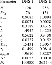
are summarized in table 1. Further details of the pseudospectral algorithm may be found in Ireland et al. (Reference Ireland, Vaithianathan, Sukheswalla, Ray and Collins2013) and Brucker et al. (Reference Brucker, Isaza, Vaithianathan and Collins2007).
Flow parameters in DNS of isotropic turbulence (arbitrary units).
 $N$
is the number of grid points in each direction,
 $Re_{\unicode[STIX]{x1D706}}\equiv u_{rms}\unicode[STIX]{x1D706}/\unicode[STIX]{x1D708}$
is the Taylor micro-scale Reynolds number,
 $u_{rms}\equiv \sqrt{(2k/3)}$
is the fluid r.m.s. fluctuating velocity,
 $k$
is the turbulent kinetic energy,
 $\unicode[STIX]{x1D708}$
is the fluid kinematic viscosity,
 $\unicode[STIX]{x1D716}\equiv 2\unicode[STIX]{x1D708}\int _{0}^{\unicode[STIX]{x1D705}_{max}}\unicode[STIX]{x1D705}^{2}E(\unicode[STIX]{x1D705})\,\text{d}\unicode[STIX]{x1D705}$
is the turbulent energy dissipation rate,
 $L\equiv 3\unicode[STIX]{x03C0}/(2k)\int _{0}^{\unicode[STIX]{x1D705}_{max}}E(\unicode[STIX]{x1D705})/\unicode[STIX]{x1D705}\,\text{d}\unicode[STIX]{x1D705}$
is the integral length scale,
 $\unicode[STIX]{x1D706}\equiv u_{rms}\sqrt{(15\unicode[STIX]{x1D708}/\unicode[STIX]{x1D716})}$
is the Taylor micro-scale,
 $\unicode[STIX]{x1D702}\equiv \unicode[STIX]{x1D708}^{3/4}/\unicode[STIX]{x1D716}^{1/4}$
is the Kolmogorov length scale,
 $T_{eddy}\equiv L/u^{\prime }$
is the large eddy turnover time,
 $\unicode[STIX]{x1D70F}_{\unicode[STIX]{x1D702}}\equiv \sqrt{(\unicode[STIX]{x1D708}/\unicode[STIX]{x1D716})}$
is the Kolmogorov time scale,
 $\unicode[STIX]{x1D705}_{max}$
is the maximum resolved wavenumber,
 $\unicode[STIX]{x0394}t$
is the time step and
 $N_{p}$
is the number of particles per Stokes number.

3.1.2 Relative-velocity correlation in CF1
For CF1, computing the diffusivity
 $\unicode[STIX]{x1D60B}_{UU}$
requires the correlation
 $\langle \unicode[STIX]{x0394}\boldsymbol{u}(\boldsymbol{r},\boldsymbol{x},0)\unicode[STIX]{x0394}\boldsymbol{u}(\boldsymbol{r},\boldsymbol{x},t)\rangle$
as input. This correlation was evaluated using DNS of forced isotropic turbulence with stationary disperse particles. Two simulation parameters that impact the computed correlation are the number of particles (thereby, pairs), and the bin size (
 $\unicode[STIX]{x0394}r$
) for pair separations. Bin size refers to the thickness of the radial shell spanning
 $r-\unicode[STIX]{x0394}r/2$
to
 $r+\unicode[STIX]{x0394}r/2$
, within which we search for pairs. An important consideration in determining the number of particles is the need to obtain converged correlations at separations
 $r\sim \unicode[STIX]{x1D702}$
, where
 $\unicode[STIX]{x1D702}$
is Kolmogorov length scale. In this regard, we varied the number of particles from
 $10^{5}$
to
 $10^{6}$
. Although smooth statistics were obtained for
 $5\times 10^{5}$
particles, we used
 $10^{6}$
particles or
 ${\sim}5\times 10^{11}$
pairs for computing the two-time correlation. It may be recalled that these particles are stationary, and are to be distinguished from those indicated in table 1 that are in motion. The ‘optimal’ bin size for pair separations is determined by balancing two competing requirements: convergence of statistics at
 $r\sim \unicode[STIX]{x1D702}$
, and the reduction of statistical noise associated with too small a bin size. We considered bin sizes varying between
 $\unicode[STIX]{x1D702}/20$
and
 $2\unicode[STIX]{x1D702}$
, and found that a bin size of
 $\unicode[STIX]{x1D702}/8$
satisfied the two constraints.
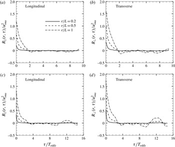
The Eulerian two-time correlation of fluid relative velocities
 $\unicode[STIX]{x1D619}(r,\unicode[STIX]{x1D70F})=\langle \unicode[STIX]{x0394}\boldsymbol{u}(\boldsymbol{r},t)\unicode[STIX]{x0394}\boldsymbol{u}(\boldsymbol{r},t+\unicode[STIX]{x1D70F})\rangle$
. The longitudinal and transverse components of
 $\unicode[STIX]{x1D619}(r,\unicode[STIX]{x1D70F})$
, i.e.
 $\unicode[STIX]{x1D619}_{||}(r,\unicode[STIX]{x1D70F})$
and
 $\unicode[STIX]{x1D619}_{\bot }(r,\unicode[STIX]{x1D70F})$
, are shown as a function of time at separations
 $r/L=0.2,0.5,1$
. Panels (a,b)
 $Re_{\unicode[STIX]{x1D706}}=76$
, and (c,d)
 $Re_{\unicode[STIX]{x1D706}}=131$
. The integral length scale
 $L=\unicode[STIX]{x03C0}/(2{u^{\prime }}^{2})\int _{0}^{\unicode[STIX]{x1D705}_{max}}E(\unicode[STIX]{x1D705})/\unicode[STIX]{x1D705}\,\text{d}\unicode[STIX]{x1D705}$
, and time scale
 $T_{eddy}=L/u_{rms}$
.

Evaluation of the two-time correlation of seen fluid relative velocities for nearly half a trillion pairs is a highly computationally intensive process. We adopted the following procedure to compute these correlations from DNS of isotropic turbulence with fixed particles. Considering two snapshots of flow separated by a time interval
 $\unicode[STIX]{x1D70F}$
in a DNS run, the longitudinal and transverse components of the product
 $\unicode[STIX]{x0394}\boldsymbol{u}(\boldsymbol{r},\boldsymbol{x},t)\unicode[STIX]{x0394}\boldsymbol{u}(\boldsymbol{r},\boldsymbol{x},t+\unicode[STIX]{x1D70F})$
for a particle pair are stored in the appropriate
 $r$
bin, and then averaged over all pairs within a bin. Next, we average the two components over pairs of flow snapshots with the same time separation
 $\unicode[STIX]{x1D70F}$
. For each value of
 $\unicode[STIX]{x1D70F}$
, we averaged over 200 such pairs of flow snapshots. In figure 1(a,b), we show the longitudinal and transverse components, respectively, of the relative-velocity correlation as a function of
 $\unicode[STIX]{x1D70F}$
at separations
 $r=L/5,L/2,L$
for
 $Re_{\unicode[STIX]{x1D706}}=76$
. Here
 $L$
is the integral length scale. The corresponding plots for
 $Re_{\unicode[STIX]{x1D706}}=131$
are shown in figure 1(c,d). The correlations at various separations are then integrated in time to yield
 $\unicode[STIX]{x1D60B}_{UU}$
for CF1.
3.1.3 Particle phase
The governing equations for the motion of a dense spherical particle smaller than the Kolmogorov length scale may be written as (Maxey & Riley Reference Maxey and Riley1983)
 $$\begin{eqnarray}\displaystyle & \displaystyle \frac{\text{d}\boldsymbol{x}_{p}}{\text{d}t}=\boldsymbol{v}_{p}, & \displaystyle\end{eqnarray}$$
 $$\begin{eqnarray}\displaystyle & \displaystyle \frac{\text{d}\boldsymbol{v}_{p}}{\text{d}t}=\frac{\boldsymbol{u}(\boldsymbol{x}_{p},t)-\boldsymbol{v}_{p}}{\unicode[STIX]{x1D70F}_{v}}, & \displaystyle\end{eqnarray}$$
where
 $\boldsymbol{x}_{p}$
and
 $\boldsymbol{v}_{p}$
are the particle position and velocity, respectively, and
 $\unicode[STIX]{x1D70F}_{v}=\unicode[STIX]{x1D70C}_{p}d_{p}^{2}/18\unicode[STIX]{x1D707}$
is the particle response time (
 $\unicode[STIX]{x1D70C}_{p}$
is the particle density,
 $d_{p}$
its diameter and
 $\unicode[STIX]{x1D707}$
is fluid dynamic viscosity). In (3.3),
 $\boldsymbol{u}(\boldsymbol{x}_{p},t)$
is the fluid velocity at the particle’s location. In the DNS runs, the seen fluid velocity is evaluated through an eighth-order Lagrange interpolation method involving a stencil of
 $8\times 8\times 8$
fluid velocities surrounding the particle location.
Temporal update of particle motion is achieved through a modified second-order Runge–Kutta (RK2) method in which the standard RK2 weights are replaced by exponential integrators as follows (Ireland et al. Reference Ireland, Vaithianathan, Sukheswalla, Ray and Collins2013):
 $$\begin{eqnarray}\displaystyle \boldsymbol{v}_{p}(t_{0}+h)=e^{-h/\unicode[STIX]{x1D70F}_{v}}\boldsymbol{v}_{p}(t_{0})+w_{1}\boldsymbol{u}_{p}[\boldsymbol{x}_{p}(t_{0})]+w_{2}\boldsymbol{u}[\boldsymbol{x}_{p}(t_{0})+\boldsymbol{v}_{p}(t_{0})h], & & \displaystyle\end{eqnarray}$$
where
 $h$
is the time step, and the exponential integrators
 $w_{1}$
and
 $w_{2}$
are given by
 $$\begin{eqnarray}\displaystyle w_{1}\equiv \left(\frac{h}{\unicode[STIX]{x1D70F}_{v}}\right)\left[\unicode[STIX]{x1D719}_{1}\left(\frac{-h}{\unicode[STIX]{x1D70F}_{v}}\right)-\unicode[STIX]{x1D719}_{2}\left(\frac{-h}{\unicode[STIX]{x1D70F}_{v}}\right)\right],\quad w_{2}\equiv \left(\frac{h}{\unicode[STIX]{x1D70F}_{v}}\right)\unicode[STIX]{x1D719}_{1}\left(\frac{-h}{\unicode[STIX]{x1D70F}_{v}}\right) & & \displaystyle\end{eqnarray}$$
 $$\begin{eqnarray}\displaystyle \unicode[STIX]{x1D719}_{1}(z)\equiv \frac{e^{z}-1}{z},\quad \unicode[STIX]{x1D719}_{2}(z)\equiv \frac{e^{z}-z-1}{z^{2}}. & & \displaystyle\end{eqnarray}$$
In the DNS runs, the particles are evolved for at least 6
 $\unicode[STIX]{x1D70F}_{v}$
for the
 $St_{\unicode[STIX]{x1D702}}=80$
particles, and 45
 $\unicode[STIX]{x1D70F}_{v}$
for the
 $St_{\unicode[STIX]{x1D702}}=10$
particles, before we begin collecting their statistics. Subsequently, the particle statistics are averaged for nearly 10
 $\unicode[STIX]{x1D70F}_{v}$
for the
 $St_{\unicode[STIX]{x1D702}}=80$
particles, and 75
 $\unicode[STIX]{x1D70F}_{v}$
for the
 $St_{\unicode[STIX]{x1D702}}=10$
particles.
3.2 Langevin simulations
Using the CF1, CF2 and CF3 closures for
 $\unicode[STIX]{x1D60B}_{UU}$
discussed in § 2, three sets of Langevin stochastic simulations were performed to evolve pair separations
 $\boldsymbol{r}$
and relative velocities
 $\boldsymbol{U}$
. The governing equations for
 $\boldsymbol{r}$
and
 $\boldsymbol{U}$
are:
 $$\begin{eqnarray}\displaystyle & \displaystyle \frac{\text{d}\boldsymbol{r}}{\text{d}t}=\boldsymbol{U} & \displaystyle\end{eqnarray}$$
 $$\begin{eqnarray}\displaystyle & \displaystyle \text{d}\boldsymbol{U}=-\frac{\boldsymbol{U}}{\unicode[STIX]{x1D70F}_{v}}\,\text{d}t+\unicode[STIX]{x1D63D}\boldsymbol{\cdot }\text{d}\unicode[STIX]{x1D652}. & \displaystyle\end{eqnarray}$$
Here,
 $\unicode[STIX]{x1D652}$
represents a Wiener process, and the diffusion matrix
 $\unicode[STIX]{x1D63D}$
can be written in terms of
 $\unicode[STIX]{x1D60B}_{UU}$
as:
 $$\begin{eqnarray}\displaystyle \unicode[STIX]{x1D63D}\boldsymbol{\cdot }\unicode[STIX]{x1D63D}^{\text{T}}=2\unicode[STIX]{x1D60B}_{UU}(r), & & \displaystyle\end{eqnarray}$$
where
 $\unicode[STIX]{x1D63D}^{\text{T}}$
is the transpose of
 $\unicode[STIX]{x1D63D}$
, and
 $\unicode[STIX]{x1D63D}$
is computed from a Cholesky decomposition of
 $\unicode[STIX]{x1D60B}_{UU}(r)$
. Simulation of Langevin equations (3.7) and (3.8) is statistically equivalent to solving the Fokker–Plank equation (2.10) for the PDF
 $\unicode[STIX]{x1D6FA}(\boldsymbol{r},\boldsymbol{U})$
.
To be able to consistently compare pair statistics from the Langevin and DNS runs, it is important that the Langevin simulations use the same turbulence parameters as those in statistically stationary DNS. Hence, inputs to Langevin runs such as the Kolmogorov and integral length scales, dissipation rate, kinematic viscosity,
 $u_{rms}$
and
 $Re_{\unicode[STIX]{x1D706}}$
are all identical to those in table 1. In particular, one also has to ensure that the model energy spectrum used in CF2 and CF3 closely matches the DNS energy spectrum. This was achieved by suitably selecting the parametric inputs to the model spectrum provided in Pope (Reference Pope2000), as follows:
 $$\begin{eqnarray}\displaystyle & \displaystyle E(\unicode[STIX]{x1D705})=C\unicode[STIX]{x1D716}^{2/3}\unicode[STIX]{x1D705}^{-5/3}f_{L}(\unicode[STIX]{x1D705}L)f_{\unicode[STIX]{x1D702}}(\unicode[STIX]{x1D705}\unicode[STIX]{x1D702}) & \displaystyle\end{eqnarray}$$
 $$\begin{eqnarray}\displaystyle & \displaystyle f_{L}(\unicode[STIX]{x1D705}L)=\left(\frac{\unicode[STIX]{x1D705}L}{[(\unicode[STIX]{x1D705}L)^{2}+c_{L}]^{1/2}}\right)^{5/3+p_{0}} & \displaystyle\end{eqnarray}$$
 $$\begin{eqnarray}\displaystyle & \displaystyle f_{\unicode[STIX]{x1D702}}(\unicode[STIX]{x1D705}\unicode[STIX]{x1D702})=\text{exp}\{-\unicode[STIX]{x1D6FD}([(\unicode[STIX]{x1D705}\unicode[STIX]{x1D702})^{4}+c_{\unicode[STIX]{x1D702}}^{4}]^{1/4}-c_{\unicode[STIX]{x1D702}})\}, & \displaystyle\end{eqnarray}$$
where
 $\unicode[STIX]{x1D6FD}=5.2$
and
 $p_{0}=2$
(Pope Reference Pope2000).
The parameters
 $c_{L}$
and
 $c_{\unicode[STIX]{x1D702}}$
are determined from the following constraints:
 $$\begin{eqnarray}\displaystyle & \displaystyle \frac{3}{2}u_{rms}^{2}=\int _{1}^{\unicode[STIX]{x1D705}_{max}}E(\unicode[STIX]{x1D705})\,\text{d}\unicode[STIX]{x1D705} & \displaystyle\end{eqnarray}$$
 $$\begin{eqnarray}\displaystyle & \displaystyle \unicode[STIX]{x1D716}=2\unicode[STIX]{x1D708}\int _{1}^{\unicode[STIX]{x1D705}_{max}}\unicode[STIX]{x1D705}^{2}E(\unicode[STIX]{x1D705})\,\text{d}\unicode[STIX]{x1D705}, & \displaystyle\end{eqnarray}$$
where
 $\unicode[STIX]{x1D716}$
is the dissipation rate, and the wavenumber limits
 $[1,\unicode[STIX]{x1D705}_{max}]$
are the same as in DNS. These wavenumber limits are also used in (2.18) and (2.19) for CF2 and CF3. The parameters
 $c_{L}$
and
 $c_{\unicode[STIX]{x1D702}}$
are numerically evaluated using the DNS values of
 $u_{rms}$
,
 $\unicode[STIX]{x1D716}$
and
 $\unicode[STIX]{x1D708}$
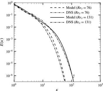
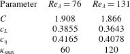
from table 1. The resulting values are shown in table 2. In figure 2, the model spectra calculated from (3.10)–(3.12) are compared with the DNS energy spectra for
 $Re_{\unicode[STIX]{x1D706}}=76$
and
 $Re_{\unicode[STIX]{x1D706}}=131$
. Good agreement is seen between the model and DNS spectra.
Comparison of the DNS and model energy spectra at
 $Re_{\unicode[STIX]{x1D706}}=76$
and
 $Re_{\unicode[STIX]{x1D706}}=131$
. The model spectrum is used to compute the CF1 and CF2 diffusivities.

Parameters for the model energy spectrum. After determining
 $c_{L}$
and
 $c_{\unicode[STIX]{x1D702}}$
, the parameter
 $C$
was adjusted to match the DNS energy spectrum. Pope (Reference Pope2000) suggested
 $C=1.5$
.

The computational domain in the Langevin simulations is a sphere of diameter
 $8L$
, where
 $L$
is the integral length scale. This domain size is sufficiently large, since particle pairs become decorrelated at separations of
 $O(L)$
for all the Stokes numbers considered in this study. A specular reflective boundary condition was imposed at the outer boundary of the domain. This meant that a particle colliding with the outer boundary is reflected back into the domain, with its velocity component tangential to the boundary unaffected, and the velocity component normal to the boundary reversed.
For each
 $St_{\unicode[STIX]{x1D702}}$
, pair statistics are averaged for at least 1000
 $\unicode[STIX]{x1D70F}_{v}$
. Such a large averaging time was necessary due to the strong dependence of the statistical errors on the sample size in Langevin simulations. Further, in order to increase the sample size at separations of the order of Kolmogorov length scale, a single pair is split into multiple, equally weighted fractional pairs whenever the separation of a pair goes below a certain value (Rani et al.
Reference Rani, Dhariwal and Koch2014). When a parent pair is split, initially the fractional pairs have the same position and velocity vectors as the parent. Each of the fractional pairs is then evolved independently, except that it only makes a fractional contribution when computing the statistics. In our simulations, splitting is executed at three different radial locations,
 $r=2\unicode[STIX]{x1D702},5\unicode[STIX]{x1D702},10\unicode[STIX]{x1D702}$
. However, fractional pairs are not split again. We found that splitting a pair into 10 equally weighted fractional pairs gave us sufficient data at the smaller separations without excessively increasing the number of pairs to be tracked. Recombination of fractional pairs when their separations exceeded the specified radial distances was not undertaken.
4 Results and discussion
Langevin and DNS runs were performed for Stokes numbers
 $St_{\unicode[STIX]{x1D702}}=10,20,40,80$
at
 $Re_{\unicode[STIX]{x1D706}}=76$
and 131. Three sets of Langevin simulations – a total of 24 simulations – were conducted corresponding to the closure forms CF1, CF2 and CF3. In each LS,
 $60\times 10^{6}$
pairs per Stokes number were considered. The number of particles in the DNS runs are provided in table 1.
The discussion of the results is presented in three subsections. In § 4.1, we first compare the three forms of the diffusivity
 $\unicode[STIX]{x1D60B}_{UU}$
. Subsequently, CF1 and the Zaichik et al. (Reference Zaichik, Simonin and Alipchenkov2003), Zaichik & Alipchenkov (Reference Zaichik and Alipchenkov2007) theory are compared in the limit of
 $St_{r}\gg 1$
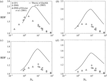
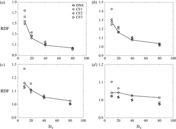
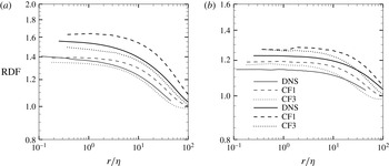
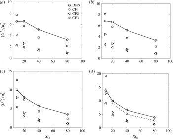
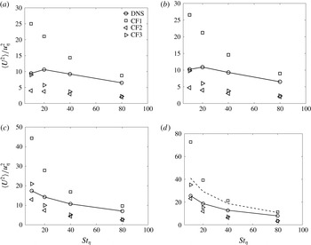
. In § 4.2, the radial distribution functions (RDFs) obtained using CF1, CF2 and CF3 are compared with the respective DNS RDFs. The trends in the RDFs obtained from the closures are explained through the moments equations of the master PDF equation (2.10). After the RDF discussion, the relative-velocity statistics and relative-velocity PDFs obtained from the LS and DNS runs are presented and compared in § 4.3. Throughout the discussion of the results, we will regard CF1 as being the most accurate among the three closures. We will elaborate on the differences in the statistical predictions of CF1 and CF2/CF3, as well as provide quantitative and qualitative explanations for the differences.
4.1 Diffusivity tensor
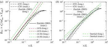
We first compare the diffusivity tensors from the three closure forms considered in this study. In addition, the CF1 and CF2 diffusivities are analysed in greater detail for pair separations in the integral range, where one can derive analytical estimates for these. Subsequently, we compare CF1 with the diffusivity closure of Zaichik & Alipchenkov (Reference Zaichik and Alipchenkov2003, Reference Zaichik and Alipchenkov2007). As CF1 is computed through DNS, it is essentially exact for
 $St_{r}\gg 1$
, presenting us an opportunity to assess the Zaichik & Alipchenkov closure in this limit. Such an analysis of their diffusivity had not been undertaken previously.
The transverse component,
 $\unicode[STIX]{x1D60B}_{UU,\bot }(r)$
, and the longitudinal component,
 $\unicode[STIX]{x1D60B}_{UU,||}(r)$
, of the diffusivity tensor for
 $St_{\unicode[STIX]{x1D702}}=10$
as a function of dimensionless pair separation
 $r/L$
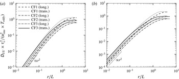
. Diffusivity tensor components for CF1, CF2 and CF3 are shown. Upper black solid line denotes CF3 transverse component, and lower grey solid line denotes CF2 transverse component. (a)
 $Re_{\unicode[STIX]{x1D706}}=76$
, and (b)
 $Re_{\unicode[STIX]{x1D706}}=131$
. Transverse and longitudinal components of
 $\unicode[STIX]{x1D60B}_{UU}$
for CF1, CF2 and CF3 in the viscous range at
 $Re_{\unicode[STIX]{x1D706}}=76$
and 131 are shown in table 3.

Transverse and longitudinal components of
 $\unicode[STIX]{x1D60B}_{UU}$
for CF1, CF2 and CF3 in the viscous range at
 $Re_{\unicode[STIX]{x1D706}}=76$
and 131. The values shown are for
 $St_{\unicode[STIX]{x1D702}}=10$
. The following notation is used:
 $\unicode[STIX]{x1D60B}_{UU,||}^{[1,2,3],\star }=[\unicode[STIX]{x1D60B}_{UU,||}^{[1,2,3]}\times \unicode[STIX]{x1D70F}_{v}^{2}/(u_{rms}^{2}\times T_{eddy})]/(r/L)^{2}$
.

In figure 3, the longitudinal and transverse components of the diffusivity for CF1, CF2 and CF3 are plotted as a function of the dimensionless separation
 $r/L$
(
 $L$
is the integral length scale). Shown in figure 3(a,b) are the diffusivity components at
 $Re_{\unicode[STIX]{x1D706}}=76$
and 131, respectively, for the
 $St_{\unicode[STIX]{x1D702}}=10$
pairs. It may be noted that
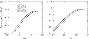
 $\unicode[STIX]{x1D60B}_{UU}\times \unicode[STIX]{x1D70F}_{v}^{2}$
is independent of the Stokes number for CF1 and CF2, but not for CF3 due to the presence of
 $W_{rms}$
on the right-hand side of (2.18) and (2.19). The diffusivities are shown for the lowest Stokes number
 $St_{\unicode[STIX]{x1D702}}=10$
, since the differences between CF2 and CF3 are more pronounced at low Stokes numbers. For Kolmogorov-scale separations, i.e.
 $r\sim \unicode[STIX]{x1D702}$
,
 $\unicode[STIX]{x1D60B}_{UU,\bot }(r)$
and
 $\unicode[STIX]{x1D60B}_{UU,||}(r)$
show an
 $r^{2}$
scaling for all three closures (numerical values of the scaling coefficients are shown in table 3). This scaling arises because for
 $r<\unicode[STIX]{x1D702}$
, the fluid velocity field may be regarded as locally linear, i.e.
 $\unicode[STIX]{x0394}\boldsymbol{u}\approx \boldsymbol{r}\boldsymbol{\cdot }\unicode[STIX]{x1D735}\boldsymbol{u}$
, which in conjunction with (2.11) gives rise to the
 $r^{2}$
scaling. At both
 $Re_{\unicode[STIX]{x1D706}}=76$
and 131, it is seen that CF3 is in reasonable agreement with CF1 for inertial range separations. However, in the transition region between the inertial and integral ranges, as well as in the integral range, CF1 is higher than CF3. The diffusivity components of CF1 exceed those of CF2 at all separations. These trends are to be expected, especially at
 $St_{\unicode[STIX]{x1D702}}=10$
, since CF3 does a better job at lower Stokes numbers than does CF2.
For integral-scale separations, i.e.
 $r\gtrsim L$
, one can perform a more detailed comparison of CF1 and CF2, since one can derive estimates for these closures in this region. It may recalled that in deriving the CF2 diffusivity expression, we assumed that the temporal change of the fluid relative velocities seen by a pair is primarily due to the passive advection of size
 $r$
eddies past the pair by large-scale eddies with velocity
 $u_{I}$
. This physical picture is valid only when
 $r/u_{I}\ll r/u_{r}=\unicode[STIX]{x1D70F}_{r}$
, i.e. when
 $r$
is small enough such that the time taken to advect the size
 $r$
eddies past the pair is smaller than their turnover time. Therefore, one expects CF2 to perform poorly at large separations.
For
 $r\gtrsim L$
, the particle pairs are effectively uncorrelated and behave like two independent particles. Consequently, the pair diffusivity is equal to twice the single particle diffusivity. Using this principle, we can write for CF1:
 $$\begin{eqnarray}\displaystyle \unicode[STIX]{x1D60B}_{UU}^{[1]}(r\gtrsim L) & = & \displaystyle \frac{1}{\unicode[STIX]{x1D70F}_{v}^{2}}\int _{-\infty }^{0}\langle \unicode[STIX]{x0394}\boldsymbol{u}(\boldsymbol{r},\boldsymbol{x},0)\unicode[STIX]{x0394}\boldsymbol{u}(\boldsymbol{r},\boldsymbol{x},t)\rangle \,\text{d}t\nonumber\\ \displaystyle & {\approx} & \displaystyle \frac{2}{\unicode[STIX]{x1D70F}_{v}^{2}}\int _{-\infty }^{0}\langle \boldsymbol{u}(\boldsymbol{x},0)\boldsymbol{u}(\boldsymbol{x},t)\rangle \,\text{d}t=\frac{2}{\unicode[STIX]{x1D70F}_{v}^{2}}u_{rms}^{2}T_{E}\unicode[STIX]{x1D6FF}_{ij},\end{eqnarray}$$
where
 $T_{E}$
is the Eulerian integral time scale.
In the case of CF2, noting that
 $\unicode[STIX]{x1D60B}_{UU,||}^{[2]}=\unicode[STIX]{x1D60B}_{UU,\bot }^{[2]}$
when
 $r\gtrsim L$
, we have
 $$\begin{eqnarray}\displaystyle \unicode[STIX]{x1D60B}_{UU}^{[2]}(r\gtrsim L) & {\approx} & \displaystyle \unicode[STIX]{x1D6FF}_{ij}\frac{2\unicode[STIX]{x03C0}^{2}}{\unicode[STIX]{x1D70F}_{v}^{2}}\sqrt{\frac{1}{(2\unicode[STIX]{x03C0})^{3}u_{rms}^{2}}}\times \frac{4}{3}\int _{0}^{\infty }\frac{E(\unicode[STIX]{x1D709})}{\unicode[STIX]{x1D709}}\,\text{d}\unicode[STIX]{x1D709}\end{eqnarray}$$
 $$\begin{eqnarray}\displaystyle & = & \displaystyle \unicode[STIX]{x1D6FF}_{ij}\frac{2\unicode[STIX]{x03C0}^{2}}{\unicode[STIX]{x1D70F}_{v}^{2}}\sqrt{\frac{1}{(2\unicode[STIX]{x03C0})^{3}u_{rms}^{2}}}\times \frac{4}{3}\times \frac{u_{rms}^{2}}{\unicode[STIX]{x03C0}}L\end{eqnarray}$$
 $$\begin{eqnarray}\displaystyle & = & \displaystyle \frac{0.53}{\unicode[STIX]{x1D70F}_{v}^{2}}u_{rms}^{2}T_{eddy}\unicode[STIX]{x1D6FF}_{ij},\end{eqnarray}$$
where we replaced
 $W_{rms}$
with
 $u_{rms}$
in (2.18) and (2.19), and the right-hand side of (4.2) is the limiting value of the right-hand side of (2.18) as
 $r\rightarrow \infty$
. We have also used the identity
 $\int _{0}^{\infty }(E(\unicode[STIX]{x1D709})/\unicode[STIX]{x1D709})\,\text{d}\unicode[STIX]{x1D709}=(u_{rms}^{2}/\unicode[STIX]{x03C0})L$
and
 $T_{eddy}=L/u_{rms}$
, where
 $L$
is the integral length scale. The ratio
 $T_{eddy}/T_{E}\sim 1.2{-}1.5$
so that from (4.1) and (4.4), the ratio
 $\unicode[STIX]{x1D60B}_{UU}^{[1]}/\unicode[STIX]{x1D60B}_{UU}^{[2]}$
is now estimated to be
 ${\sim}2.5{-}3.2$
for
 $r\gtrsim L$
.
In figure 3, for
 $r\gtrsim L$
, we see that
 $\unicode[STIX]{x1D60B}_{UU}^{[1]}/\unicode[STIX]{x1D60B}_{UU}^{[2]}\approx 2.05$
when
 $Re_{\unicode[STIX]{x1D706}}=76$
, and
 ${\approx}3.45$
when
 $Re_{\unicode[STIX]{x1D706}}=131$
, in accordance with the preceding scaling estimate. Further,
 $\unicode[STIX]{x1D60B}_{UU}^{[1]}/\unicode[STIX]{x1D60B}_{UU}^{[3]}\approx 1.5$
when
 $Re_{\unicode[STIX]{x1D706}}=76$
, and
 ${\approx}2.29$
when
 $Re_{\unicode[STIX]{x1D706}}=131$
. The lower values of
 $\unicode[STIX]{x1D60B}_{UU}^{[1]}/\unicode[STIX]{x1D60B}_{UU}^{[3]}$
are because CF3 exceeds CF2 for smaller
 $St_{\unicode[STIX]{x1D702}}$
. We will also see in § 4.3 that for
 $r\gtrsim L$
, the pair relative-velocity variance computed using CF1 is in good agreement with an analytical expression for the relative-velocity variance of uncorrelated pairs (Pan & Padoan Reference Pan and Padoan2013). However, both CF2 and CF3 underpredict this analytical variance by nearly the same factors as
 $\unicode[STIX]{x1D60B}_{UU}^{[1]}/\unicode[STIX]{x1D60B}_{UU}^{[2]}$
and
 $\unicode[STIX]{x1D60B}_{UU}^{[1]}/\unicode[STIX]{x1D60B}_{UU}^{[3]}$
for
 $r\gtrsim L$
in figure 3.
In figure 4, we compare only CF2 and CF3 for the highest Stokes number considered. Figures 4(a,b) show the diffusion tensor components for the
 $St_{\unicode[STIX]{x1D702}}=80$
particles at
 $Re_{\unicode[STIX]{x1D706}}=76$
and 131, respectively. At high Stokes numbers,
 $W_{rms}\approx u_{rms}$
, so that one expects CF2 and CF3 to have similar diffusivities, which is confirmed in figure 4.
Transverse component,
 $\unicode[STIX]{x1D60B}_{UU,\bot }(r)$
, and longitudinal component,
 $\unicode[STIX]{x1D60B}_{UU,||}(r)$
, of the diffusion coefficient tensor for
 $St_{\unicode[STIX]{x1D702}}=80$
as a function of dimensionless pair separation
 $r/L$
at: (a)
 $Re_{\unicode[STIX]{x1D706}}=76$
and (b)
 $Re_{\unicode[STIX]{x1D706}}=131$
. CF2 and CF3 diffusivities are compared.

We now present a comparative analysis of CF1 and the Zaichik & Alipchenkov (Reference Zaichik and Alipchenkov2003, Reference Zaichik and Alipchenkov2007) closures. As already mentioned, CF1 may be regarded as ‘exact’ for
 $St_{r}\gg 1$
. In this limit, the Zaichik & Alipchenkov diffusivity in
 $\boldsymbol{U}$
-space may be written as:
 $$\begin{eqnarray}\displaystyle \unicode[STIX]{x1D60B}_{UU}^{Zaichik}=\frac{1}{\unicode[STIX]{x1D70F}_{v}}\frac{T_{Lr}}{\unicode[STIX]{x1D70F}_{v}+T_{Lr}}\unicode[STIX]{x1D61A}(\boldsymbol{r})\rightarrow \frac{1}{\unicode[STIX]{x1D70F}_{v}^{2}}\unicode[STIX]{x1D61A}(\boldsymbol{r})T_{Lr}, & & \displaystyle\end{eqnarray}$$
where
 $\unicode[STIX]{x1D61A}(\boldsymbol{r})$
is the Eulerian structure function tensor, and
 $T_{Lr}$
is the Lagrangian two-point time scale at separation
 $r$
. We can now calculate
 $\unicode[STIX]{x1D60B}_{UU}^{Zaichik}$
using the well-known scaling expressions of
 $\unicode[STIX]{x1D61A}(r)$
and
 $T_{Lr}$
for separations
 $r$
in the dissipative, inertial and integral ranges. The expressions for the longitudinal and transverse components of
 $\unicode[STIX]{x1D61A}(r)$
are (Zaichik & Alipchenkov Reference Zaichik and Alipchenkov2003):
 $$\begin{eqnarray}\displaystyle & \displaystyle \text{Viscous range: }\unicode[STIX]{x1D61A}_{||}(r)=\frac{\unicode[STIX]{x1D716}r^{2}}{15\unicode[STIX]{x1D708}};\unicode[STIX]{x1D61A}_{\bot }(r)=\frac{2\unicode[STIX]{x1D716}r^{2}}{15\unicode[STIX]{x1D708}} & \displaystyle\end{eqnarray}$$
 $$\begin{eqnarray}\displaystyle & \displaystyle \text{Inertial range: }\unicode[STIX]{x1D61A}_{||}(r)=C_{1}(\unicode[STIX]{x1D716}r)^{2/3};\unicode[STIX]{x1D61A}_{\bot }(r)={\textstyle \frac{4}{3}}C_{1}(\unicode[STIX]{x1D716}r)^{2/3} & \displaystyle\end{eqnarray}$$
 $$\begin{eqnarray}\displaystyle & \displaystyle \text{Integral range: }\unicode[STIX]{x1D61A}_{||}(r)=\unicode[STIX]{x1D61A}_{\bot }(r)=2u_{rms}^{2}, & \displaystyle\end{eqnarray}$$
where
 $C_{1}=2.0$
.
The corresponding expressions for
 $T_{Lr}(r)$
are also provided in Zaichik & Alipchenkov (Reference Zaichik and Alipchenkov2003). It is, however, relevant to elaborate on
 $T_{Lr}$
in the dissipative range. To determine
 $T_{Lr}$
in this range, Zaichik & Alipchenkov (Reference Zaichik and Alipchenkov2003) approximated the fluid relative velocity as being linear in the separation vector:
 $\unicode[STIX]{x0394}\boldsymbol{u}\approx \boldsymbol{r}\boldsymbol{\cdot }\unicode[STIX]{x1D735}\boldsymbol{u}$
. Accordingly, the viscous
 $T_{Lr}$
would need to be found in terms of the correlation time scales,
 $\unicode[STIX]{x1D70F}_{\unicode[STIX]{x1D70E}}$
and
 $\unicode[STIX]{x1D70F}_{\unicode[STIX]{x1D714}}$
, of the strain-rate and rotation-rate tensors constituting the velocity gradient. Zaichik et al. (Reference Zaichik, Simonin and Alipchenkov2003) considered
 $\unicode[STIX]{x1D70F}_{\unicode[STIX]{x1D70E}}=\unicode[STIX]{x1D70F}_{\unicode[STIX]{x1D714}}=A_{1}\unicode[STIX]{x1D70F}_{\unicode[STIX]{x1D702}}$
, where
 $\unicode[STIX]{x1D70F}_{\unicode[STIX]{x1D702}}$
is the Kolmogorov time scale. Subsequently, Zaichik & Alipchenkov (Reference Zaichik and Alipchenkov2007) reconsidered this analysis with separate forms for
 $\unicode[STIX]{x1D70F}_{\unicode[STIX]{x1D70E}}$
and
 $\unicode[STIX]{x1D70F}_{\unicode[STIX]{x1D714}}$
. We can now write the expressions for
 $T_{Lr}(r)$
as:
 $$\begin{eqnarray}\displaystyle \left.\begin{array}{@{}c@{}}\text{Viscous range [Z }\& \text{ A (2003)]: }T_{Lr}=A_{1}\unicode[STIX]{x1D70F}_{\unicode[STIX]{x1D702}}\\ \text{Viscous range [Z }\& \text{ A (2007)]: }\unicode[STIX]{x1D70F}_{\unicode[STIX]{x1D70E}}=A_{\unicode[STIX]{x1D70E}}\unicode[STIX]{x1D70F}_{\unicode[STIX]{x1D702}};\unicode[STIX]{x1D70F}_{\unicode[STIX]{x1D714}}=A_{\unicode[STIX]{x1D714}}\unicode[STIX]{x1D70F}_{\unicode[STIX]{x1D702}}\end{array}\right\} & & \displaystyle\end{eqnarray}$$
 $$\begin{eqnarray}\displaystyle & \displaystyle T_{Lr,||}=\unicode[STIX]{x1D70F}_{\unicode[STIX]{x1D70E}};T_{Lr,\bot }=\left(\frac{\unicode[STIX]{x1D70F}_{\unicode[STIX]{x1D70E}}}{5}+\frac{\unicode[STIX]{x1D70F}_{\unicode[STIX]{x1D714}}}{3}\right) & \displaystyle\end{eqnarray}$$
 $$\begin{eqnarray}\displaystyle & \displaystyle \text{Inertial range: }T_{Lr}=A_{2}\unicode[STIX]{x1D716}^{-1/3}r^{2/3} & \displaystyle\end{eqnarray}$$
 $$\begin{eqnarray}\displaystyle & \displaystyle \text{Integral range: }T_{Lr}=T_{L}, & \displaystyle\end{eqnarray}$$
where
 $A_{1}=\sqrt{5}$
(Lundgren Reference Lundgren1981),
 $A_{\unicode[STIX]{x1D70E}}=2.3$
,
 $A_{\unicode[STIX]{x1D714}}=7.2$
,
 $A_{2}=1/\sqrt{6}$
and
 $T_{L}$
is the Lagrangian integral time scale. The relationship between the viscous range
 $T_{Lr,\bot }$
and
 $\unicode[STIX]{x1D70F}_{\unicode[STIX]{x1D70E}}$
and
 $\unicode[STIX]{x1D70F}_{\unicode[STIX]{x1D714}}$
in (4.10) was obtained from the Brunk, Koch & Lion (Reference Brunk, Koch and Lion1997) study of tracer pair diffusion and coagulation in isotropic random velocity fields.
Comparison of CF1 of
 $\unicode[STIX]{x1D60B}_{UU}$
with the diffusivity of Zaichik & Alipchenkov (Reference Zaichik and Alipchenkov2003, Reference Zaichik and Alipchenkov2007) in the limit
 $St_{r}\gg 1$
.
 $\unicode[STIX]{x1D60B}_{UU,||}(r)$
and
 $\unicode[STIX]{x1D60B}_{UU,\bot }(r)$
are the longitudinal and transverse components of
 $\unicode[STIX]{x1D60B}_{UU}$
, respectively. ‘Zaichik’ refers to the diffusivity calculated from (4.13)–(4.15). Diffusion coefficient is plotted as a function of dimensionless pair separation
 $r/L$
at: (a)
 $Re_{\unicode[STIX]{x1D706}}=76$
, and (b)
 $Re_{\unicode[STIX]{x1D706}}=131$
. Also shown in panel (a) are the diffusivities obtained using the two scaling expressions for the viscous time scale: (4.6) and (4.9), and (4.6) and (4.10). In (b) we show diffusivities obtained from the scaling expressions in the inertial subrange: (4.7) and (4.11). For the viscous range, two forms of scaling expressions are plotted: one in which strain rate and rotation rate have identical time scales (
 $\unicode[STIX]{x1D70F}_{\unicode[STIX]{x1D70E}}=\unicode[STIX]{x1D70F}_{\unicode[STIX]{x1D714}}$
), and the second in which they are different (
 $\unicode[STIX]{x1D70F}_{\unicode[STIX]{x1D70E}}\neq \unicode[STIX]{x1D70F}_{\unicode[STIX]{x1D714}}$
). For the latter, these time scales are obtained from Zaichik & Alipchenkov (Reference Zaichik and Alipchenkov2007).

Conveniently, the scaling expressions given in Zaichik et al. (Reference Zaichik, Simonin and Alipchenkov2003) can be combined into unified forms for the entire range of turbulent scales. These are (Zaichik, Simonin & Alipchenkov Reference Zaichik, Simonin and Alipchenkov2006; Pan & Padoan Reference Pan and Padoan2013):
 $$\begin{eqnarray}\displaystyle & \displaystyle \unicode[STIX]{x1D61A}_{||}(r)=2u_{rms}^{2}\left[1-\exp \left(-\frac{(r/\unicode[STIX]{x1D702})}{(15C_{K})^{3/4}}\right)\right]^{4/3}\left[\frac{(r/\unicode[STIX]{x1D702})^{4}}{(r/\unicode[STIX]{x1D702})^{4}+(2u_{rms}^{2}/(C_{K}u_{\unicode[STIX]{x1D702}}^{2}))^{6}}\right]^{1/6} & \displaystyle\end{eqnarray}$$
 $$\begin{eqnarray}\displaystyle & \displaystyle \unicode[STIX]{x1D61A}_{\bot }(r)=2u_{rms}^{2}\left[1-\exp \left(-\frac{(r/\unicode[STIX]{x1D702})^{4/3}}{(15C_{Kn}/2)}\right)\right]\left[\frac{(r/\unicode[STIX]{x1D702})^{4}}{(r/\unicode[STIX]{x1D702})^{4}+(2u_{rms}^{2}/(C_{Kn}u_{\unicode[STIX]{x1D702}}^{2}))^{6}}\right]^{1/6} & \displaystyle\end{eqnarray}$$
 $$\begin{eqnarray}\displaystyle & \displaystyle T_{Lr}(r)=T_{L}\left[1-\exp \left(-\left(\frac{C_{T}}{\sqrt{5}}\right)^{3/2}\left(\frac{r}{\unicode[STIX]{x1D702}}\right)\right)\right]^{-2/3}\left[\frac{(r/\unicode[STIX]{x1D702})^{4}}{(r/\unicode[STIX]{x1D702})^{4}+(T_{L}/(C_{T}\unicode[STIX]{x1D70F}_{\unicode[STIX]{x1D702}}))^{6}}\right]^{1/6},\qquad & \displaystyle\end{eqnarray}$$
where
 $u_{\unicode[STIX]{x1D702}}$
is the Kolmogorov velocity scale,
 $C_{K}=2$
,
 $C_{Kn}\approx 2.5$
and
 $C_{T}=0.4$
.
We now compare CF1 with
 $\unicode[STIX]{x1D60B}_{UU}^{Zaichik}(r)$
in figure 5. The latter is computed from (4.5) in conjunction with (4.13)–(4.15). The agreement between CF1 and
 $\unicode[STIX]{x1D60B}_{UU}^{Zaichik}$
is good at
 $Re_{\unicode[STIX]{x1D706}}=76$
and reasonable at
 $Re_{\unicode[STIX]{x1D706}}=131$
. In the dissipative range,
 $\unicode[STIX]{x1D60B}_{UU,||}^{Zaichik}$
and
 $\unicode[STIX]{x1D60B}_{UU,\bot }^{Zaichik}$
are higher than their CF1 counterparts at
 $Re_{\unicode[STIX]{x1D706}}=131$
. It is to be noted that in the integral range
 $T_{L}\approx T_{E}/1.1$
is used (Pan & Padoan Reference Pan and Padoan2013), where
 $T_{E}$
is the Eulerian integral time scale evaluated from DNS using
 $T_{E}=u_{rms}^{2}\times \int _{0}^{\infty }\unicode[STIX]{x1D70C}(t)\,\text{d}t$
. Here
 $\unicode[STIX]{x1D70C}(t)$
is the Eulerian autocorrelation of fluid velocities. The unified expressions (4.13)–(4.15) result in a rather broad inertial region at
 $Re_{\unicode[STIX]{x1D706}}=76$
. Moreover, at
 $Re_{\unicode[STIX]{x1D706}}=131$
, it is surprising that the Zaichik transverse component falls below even the CF1 longitudinal component in the inertial region. These trends suggest that the combined expressions need improvement in the inertial range, as well as in the transition region between the inertial and integral ranges. To elaborate on this aspect, in figure 5(b), we also plot the scaling expressions
 $\unicode[STIX]{x1D61A}_{||}(r)\times T_{Lr}$
and
 $\unicode[STIX]{x1D61A}_{\bot }(r)\times T_{Lr}$
for inertial range
 $r$
, computed from (4.7) and (4.11). These are in good agreement with
 $\unicode[STIX]{x1D60B}_{UU,||}^{[1]}$
and
 $\unicode[STIX]{x1D60B}_{UU,\bot }^{[1]}$
in the inertial region, suggesting that the scaling laws for the inertial subrange are accurate, but the unified expressions fail to accurately capture the transition from the inertial- to integral-scale separations. The effects of the unified expressions on the RDF predictions of Zaichik et al. (Reference Zaichik, Simonin and Alipchenkov2003) are elaborated in § 4.2.
We also explored the differences between the viscous time scale of Zaichik & Alipchenkov (Reference Zaichik and Alipchenkov2003) (4.9), and of Zaichik & Alipchenkov (Reference Zaichik and Alipchenkov2007) (4.10). The transverse and longitudinal diffusivities obtained from these two forms of the viscous time scale are plotted in figure 5(a). It can be seen that the longitudinal diffusivities from the two Zaichik & Alipchenkov studies are identical, and are in good agreement with
 $\unicode[STIX]{x1D60B}_{UU,||}^{[1]}(r)$
. The transverse diffusivity corresponding to (4.9) is also in good agreement with
 $\unicode[STIX]{x1D60B}_{UU,\bot }^{[1]}(r)$
, but that computed using (4.10) significantly overpredicts the current
 $\unicode[STIX]{x1D60B}_{UU,\bot }^{[1]}(r)$
. The transverse diffusivity based on a Lagrangian time scale (Zaichik & Alipchenkov Reference Zaichik and Alipchenkov2007) exceeding that based on an Eulerian time scale (CF1) is evidently problematic. The viscous time scale
 $T_{Lr,\bot }=(\unicode[STIX]{x1D70F}_{\unicode[STIX]{x1D70E}}/5+\unicode[STIX]{x1D70F}_{\unicode[STIX]{x1D714}}/3)$
arises in the context of tracer pair diffusion in isotropic random velocity fields (Brunk et al.
Reference Brunk, Koch and Lion1997). It is not clear if this time scale can be applied for isotropic turbulence. We believe that the rather simple scaling
 $T_{Lr}=A_{1}\unicode[STIX]{x1D70F}_{\unicode[STIX]{x1D702}}$
with
 $A_{1}=\sqrt{2}$
(Lundgren Reference Lundgren1981) is sufficiently accurate, obviating the need for the more complex form presented in Zaichik & Alipchenkov (Reference Zaichik and Alipchenkov2007) at least for Stokes numbers greater than one.
4.2 Radial distribution function
Radial distribution function as a function of
 $St_{\unicode[STIX]{x1D702}}$
at specific separations: (a)
 $r/\unicode[STIX]{x1D702}=6$
, (b)
 $r/\unicode[STIX]{x1D702}=12$
, (c)
 $r/\unicode[STIX]{x1D702}=18$
and (d)
 $r/\unicode[STIX]{x1D702}=24$
. In each plot, squares and circles represent data from CF1 and current DNS at
 $Re_{\unicode[STIX]{x1D706}}=76$
; triangles represent DNS data of Février, Simonin & Legendre (Reference Février, Simonin and Legendre2001) at
 $Re_{\unicode[STIX]{x1D706}}=69$
. Solid line represents data from Zaichik et al. (Reference Zaichik, Simonin and Alipchenkov2003) theory for
 $Re_{\unicode[STIX]{x1D706}}=69$
.

Radial distribution function versus
 $St_{\unicode[STIX]{x1D702}}$
at separation
 $r/\unicode[STIX]{x1D702}=1$
. Squares and circles represent data from CF1 and current DNS at
 $Re_{\unicode[STIX]{x1D706}}=76$
. Curve 1 represents Zaichik et al. (Reference Zaichik, Simonin and Alipchenkov2003) theory for
 $Re_{\unicode[STIX]{x1D706}}=69$
; and Curve 2 represents Zaichik & Alipchenkov (Reference Zaichik and Alipchenkov2009) theory for
 $Re_{\unicode[STIX]{x1D706}}=75$
.

The RDF is a well-established measure of particle clustering. In figure 6, the RDF is presented as a function of
 $St_{\unicode[STIX]{x1D702}}$
at four separations
 $r/\unicode[STIX]{x1D702}=6,12,18$
and 24. The results from the CF1-based Langevin simulations are compared with the data from the current DNS, the Février et al. (Reference Février, Simonin and Legendre2001) DNS, and also with the results from the Zaichik et al. (Reference Zaichik, Simonin and Alipchenkov2003) theory. The Février et al. (Reference Février, Simonin and Legendre2001) data were for
 $Re_{\unicode[STIX]{x1D706}}=69$
, while the current DNS data are for
 $Re_{\unicode[STIX]{x1D706}}=76$
. There is excellent agreement between the CF1 RDF and the two sets of DNS RDFs at all four separations, particularly for
 $St_{\unicode[STIX]{x1D702}}>10$
. The RDFs obtained from the Zaichik & Alipchenkov (Reference Zaichik and Alipchenkov2003) theory are significantly higher than the DNS values at all separations.
In subsequent studies (Zaichik & Alipchenkov Reference Zaichik and Alipchenkov2007, Reference Zaichik and Alipchenkov2009), they endeavoured to improve the theory, principally by dropping their earlier assumption that the Lagrangian correlation time scales of the strain-rate and rotation-rate tensors are equal. For
 $St_{\unicode[STIX]{x1D702}}<1$
, the power-law exponent
 $C_{3}$
of the RDF (
 ${\sim}(\unicode[STIX]{x1D702}/r)^{C_{3}}$
for
 $r\ll \unicode[STIX]{x1D702}$
) obtained using the modified theory showed good agreement with the RDF exponents computed using DNS and the theory of Chun et al. (Reference Chun, Koch, Rani, Ahluwalia and Collins2005). In figure 7, we compare the RDFs from CF1 and the current DNS with those from the Zaichik & Alipchenkov (Reference Zaichik and Alipchenkov2009) theory at separation
 $r/\unicode[STIX]{x1D702}=1$
. Also shown are the RDF values from Zaichik & Alipchenkov (Reference Zaichik and Alipchenkov2003). We observe that the RDFs computed using their modified theory move closer to, but still overpredict, the current DNS data for
 $St_{\unicode[STIX]{x1D702}}\gtrsim 10$
.
We attribute this overprediction to two features of the Zaichik & Alipchenkov theory. First, we believe that the discrepancy may principally be due to the way in which the RDFs were computed in their study, i.e. through the solution of the transport equations for the moments of the PDF
 $\unicode[STIX]{x1D6FA}(\boldsymbol{r},\boldsymbol{U})$
(see (2.10)). This aspect is elaborated in the following discussion.
Considering the pair PDF
 $\unicode[STIX]{x1D6FA}(\boldsymbol{r},\boldsymbol{U})$
, the moments of interest are
 $$\begin{eqnarray}\displaystyle & \displaystyle \unicode[STIX]{x1D714}(\boldsymbol{r})=\int \unicode[STIX]{x1D6FA}(\boldsymbol{r},\boldsymbol{U})\,\text{d}\boldsymbol{U} & \displaystyle\end{eqnarray}$$
 $$\begin{eqnarray}\displaystyle & \displaystyle \langle U_{i}\rangle =\frac{1}{\unicode[STIX]{x1D714}(\boldsymbol{r})}\int U_{i}\unicode[STIX]{x1D6FA}(\boldsymbol{r},\boldsymbol{U})\,\text{d}\boldsymbol{U} & \displaystyle\end{eqnarray}$$
 $$\begin{eqnarray}\displaystyle & \displaystyle \langle U_{i}U_{j}\rangle =\frac{1}{\unicode[STIX]{x1D714}(\boldsymbol{r})}\int U_{i}U_{j}\unicode[STIX]{x1D6FA}(\boldsymbol{r},\boldsymbol{U})\,\text{d}\boldsymbol{U}. & \displaystyle\end{eqnarray}$$
The governing equation for the marginal PDF
 $\unicode[STIX]{x1D714}(\boldsymbol{r})$
is obtained by integrating (2.10) over the
 $\boldsymbol{U}$
space, and that for
 $\langle U_{i}\rangle$
is obtained by premultiplying (2.10) with
 $U_{i}/\unicode[STIX]{x1D714}(\boldsymbol{r})$
and then integrating over
 $\boldsymbol{U}$
. Similarly, one also obtains the transport equation for
 $\langle U_{i}U_{j}\rangle$
by taking the second relative-velocity moments of (2.10). It may be noted that
 $\unicode[STIX]{x1D714}(r)$
and the RDF
 $g(r)$
are related through
 $g(r)=\unicode[STIX]{x1D714}(r)/\unicode[STIX]{x1D714}(r\rightarrow \infty )$
.
The transport equation for
 $\unicode[STIX]{x1D714}(\boldsymbol{r})$
is given by (Zaichik & Alipchenkov Reference Zaichik and Alipchenkov2003)
 $$\begin{eqnarray}\displaystyle \frac{\unicode[STIX]{x2202}\unicode[STIX]{x1D714}}{\unicode[STIX]{x2202}t}+\frac{\unicode[STIX]{x2202}(\unicode[STIX]{x1D714}U_{k})}{\unicode[STIX]{x2202}r_{k}}=0, & & \displaystyle\end{eqnarray}$$
which only tells us that at steady state, in isotropic turbulence
 $\langle U_{i}\rangle =0$
. In fact,
 $\unicode[STIX]{x1D714}(\boldsymbol{r})$
has to be obtained from the
 $\langle U_{i}\rangle$
equation. However, when one attempts to solve the equations for the first or higher moments (of
 $U_{i}$
), one encounters additional closure problems. For instance, the equation for
 $\langle U_{i}\rangle$
contains the unclosed moment
 $\langle U_{i}U_{j}\rangle$
(Zaichik & Alipchenkov Reference Zaichik and Alipchenkov2003). To obtain
 $\langle U_{i}U_{j}\rangle$
, one writes the transport equation for
 $\langle U_{i}U_{j}\rangle$
, which in turn involves
 $\langle U_{i}U_{j}U_{k}\rangle$
, and so on. This leads to an infinite hierarchy of moments equations, which is typically broken by introducing further closure approximations. For example, in Zaichik & Alipchenkov (Reference Zaichik and Alipchenkov2003), a ‘quasi-Gaussian’ approximation (QGA) was introduced for
 $U_{i}$
, allowing them to approximate the fourth-order moments of relative velocities in terms of the second-order moments. Even for
 $St_{\unicode[STIX]{x1D702}}\gg 1$
particles, QGA may be problematic for separations
 $r<L$
, where the relative-velocity PDF is far from Gaussian and the second moments may be transported over distances much larger than
 $r$
. Further, as pointed out by Bragg & Collins (Reference Bragg and Collins2014b
), for larger Stokes numbers, the PDF of
 $\boldsymbol{U}$
in the dissipation range may be extremely intermittent. These closure approximations may be an important contributing factor to the errors in the RDFs of Zaichik & Alipchenkov. A more detailed analysis of the predictions of the Zaichik & Alipchenkov theory may be found in Bragg & Collins (Reference Bragg and Collins2014a
,Reference Bragg and Collins
b
).
The second reason for the differences between the DNS and Zaichik RDFs in figure 6 may be the use of the unified expressions for the diffusivity in their theory. As shown in figure 5(b) and in the discussion following (4.5), the unified expressions used for
 $\unicode[STIX]{x1D61A}$
and
 $T_{Lr}$
need improvement in the inertial region, as well as the transition region between the inertial and integral ranges. The discrepancies in the diffusivity in these regions may have contributed to the overprediction of RDFs by their theory, since the high
 $St_{\unicode[STIX]{x1D702}}$
particles preferentially respond to these scales.
RDFs from Langevin simulations (CF1, CF2 and CF3) and from DNS as a function of dimensionless pair separation
 $r/\unicode[STIX]{x1D702}$
for the indicated values of
 $St_{\unicode[STIX]{x1D702}}=10$
, 80. (a,b)
 $Re_{\unicode[STIX]{x1D706}}=76$
, and (c,d)
 $Re_{\unicode[STIX]{x1D706}}=131$
.

Figure 8(a,b) compare the RDFs obtained using CF1, CF2 and CF3 with the DNS RDF for
 $St_{\unicode[STIX]{x1D702}}=10$
and 80, respectively, at
 $Re_{\unicode[STIX]{x1D706}}=76$
. Figure 8(c,d) show the corresponding plots at
 $Re_{\unicode[STIX]{x1D706}}=131$
. For
 $St_{\unicode[STIX]{x1D702}}=10$
, the CF1 and CF3 RDFs show good qualitative and quantitative agreement with the DNS RDF at both Reynolds numbers. For
 $St_{\unicode[STIX]{x1D702}}=10$
and both
 $Re_{\unicode[STIX]{x1D706}}$
, CF2 overpredicts clustering as compared to DNS for both viscous and inertial separations. For
 $St_{\unicode[STIX]{x1D702}}=80$
, all the RDFs are close to unity, suggesting only a small amount of particle clustering. One also notices that the RDFs plateau, i.e. become essentially independent of
 $r$
, for separations in the inertial subrange. The plateauing is delayed, i.e. starts at smaller separations, for the
 $St_{\unicode[STIX]{x1D702}}=10$
pairs than for the
 $St_{\unicode[STIX]{x1D702}}=80$
pairs. The above RDF trends can be deduced by considering the governing equation for
 $\langle U_{i}\rangle$
, given by:
 $$\begin{eqnarray}\displaystyle \frac{\unicode[STIX]{x2202}\langle U_{i}\rangle }{\unicode[STIX]{x2202}t}+\frac{\unicode[STIX]{x2202}\langle U_{i}\rangle \langle U_{j}\rangle }{\unicode[STIX]{x2202}r_{j}}+\frac{\unicode[STIX]{x2202}\langle U_{i}^{\prime }U_{j}^{\prime }\rangle }{\unicode[STIX]{x2202}r_{j}}=-\frac{\langle U_{i}\rangle }{\unicode[STIX]{x1D70F}_{v}}-\langle U_{i}^{\prime }U_{j}^{\prime }\rangle \frac{\unicode[STIX]{x2202}\ln \unicode[STIX]{x1D714}(\boldsymbol{r})}{\unicode[STIX]{x2202}r_{j}}. & & \displaystyle\end{eqnarray}$$
For isotropic turbulence,
 $\langle U_{i}\rangle =0$
, so that (4.20) becomes
 $$\begin{eqnarray}\displaystyle \frac{\unicode[STIX]{x2202}\langle U_{\unicode[STIX]{x1D6FC}}^{\prime }U_{\unicode[STIX]{x1D6FC}}^{\prime }\rangle }{\unicode[STIX]{x2202}r_{\unicode[STIX]{x1D6FC}}}=-\langle U_{\unicode[STIX]{x1D6FC}}^{\prime }U_{\unicode[STIX]{x1D6FC}}^{\prime }\rangle \frac{\unicode[STIX]{x2202}\ln \unicode[STIX]{x1D714}(\boldsymbol{r})}{\unicode[STIX]{x2202}r_{\unicode[STIX]{x1D6FC}}}, & & \displaystyle\end{eqnarray}$$
where
 $\unicode[STIX]{x1D6FC}=1,2,3$
(repeated
 $\unicode[STIX]{x1D6FC}$
does not denote a summation). We can now write
 $$\begin{eqnarray}\displaystyle \frac{\unicode[STIX]{x2202}\ln \langle U_{\unicode[STIX]{x1D6FC}}^{\prime }U_{\unicode[STIX]{x1D6FC}}^{\prime }\rangle }{\unicode[STIX]{x2202}r_{\unicode[STIX]{x1D6FC}}}+\frac{\unicode[STIX]{x2202}\ln \unicode[STIX]{x1D714}(\boldsymbol{r})}{\unicode[STIX]{x2202}r_{\unicode[STIX]{x1D6FC}}}=0, & & \displaystyle\end{eqnarray}$$
which yields the rather elegant result for
 $St_{r}\gg 1$
pairs:
 $$\begin{eqnarray}\displaystyle \unicode[STIX]{x1D714}(r)=C(St)\langle U_{\unicode[STIX]{x1D6FC}}^{\prime }U_{\unicode[STIX]{x1D6FC}}^{\prime }\rangle ^{-1}(r)=C(St)\langle U^{2}\rangle ^{-1}, & & \displaystyle\end{eqnarray}$$
where
 $C(St)$
is an unknown coefficient that depends on the Stokes number. This dependence of the RDF may be contrasted with the power-law scaling of the RDF for the
 $St_{\unicode[STIX]{x1D702}}\ll 1$
particles at separations
 $r\lesssim \unicode[STIX]{x1D702}$
(Chun et al.
Reference Chun, Koch, Rani, Ahluwalia and Collins2005):
 $$\begin{eqnarray}\displaystyle g(r)=C_{2}\left(\frac{r}{\unicode[STIX]{x1D702}}\right)^{-C_{3}}, & & \displaystyle\end{eqnarray}$$
where
 $C_{3}\sim St_{\unicode[STIX]{x1D702}}$
.
 $\langle U^{2}\rangle /u_{rms}^{2}$
as a function of
 $r/L$
for all Stokes numbers. (a)
 $Re_{\unicode[STIX]{x1D706}}=76$
and (b)
 $Re_{\unicode[STIX]{x1D706}}=131$
. Lines denote CF1 and symbols denote CF2.

From (4.21), we can readily see that the flattening of the RDFs is related to the flattening of
 $\langle U^{2}\rangle$
. By reading figure 8(a,c) in conjunction with figure 9(a,b), one can see that the delayed plateauing of RDF for the
 $St_{\unicode[STIX]{x1D702}}=10$
particles is related to the correspondingly delayed plateauing of
 $\langle U^{2}\rangle$
at both Reynolds numbers. The overprediction of RDFs by CF2 for the viscous and inertial separations may also be inferred from (4.23) which shows that the RDF is inversely proportional to the relative-velocity variance. Since CF2 yields the lowest variances among the three closures, we see the associated overprediction of RDFs.
Figure 9(a,b) also suggest that
 $\langle U^{2}\rangle$
remains finite as the separation
 $r\rightarrow 0$
for all the
 $St_{\unicode[STIX]{x1D702}}$
considered in this study. Bec et al. (Reference Bec, Biferale, Cencini, Lanotte and Toschi2010) performed a DNS study of the low-order velocity structure functions of inertial particles in isotropic turbulence, and found that the structure functions were independent of separation in the dissipation range for
 $St_{\unicode[STIX]{x1D702}}>7$
. In Rani et al. (Reference Rani, Dhariwal and Koch2014), we had classified high-inertia particle pairs into ‘lingerers’ and ‘flyers’. Lingerers are low-relative-velocity particles that are highly correlated and remain correlated far longer than the time scales of fluid that influence their relative motion. Flyers are uncorrelated particles with large relative velocities, i.e. they undergo essentially ballistic motion so that their relative motion is unaffected by fluid eddies with sizes comparable to the pair separation. Flyers are responsible for maintaining a finite
 $\langle U^{2}\rangle$
as the separation
 $r\rightarrow 0$
.
RDF versus
 $St_{\unicode[STIX]{x1D702}}$
at
 $Re_{\unicode[STIX]{x1D706}}=76$
and at specific pair separations: (a)
 $r/\unicode[STIX]{x1D702}=1$
, (b)
 $r/\unicode[STIX]{x1D702}=11$
, (c)
 $r/\unicode[STIX]{x1D702}=22$
and (d)
 $r/\unicode[STIX]{x1D702}=44$
(
 ${\approx}L$
). CF1, CF2, CF3, and DNS are compared.

RDF versus
 $St_{\unicode[STIX]{x1D702}}$
at
 $Re_{\unicode[STIX]{x1D706}}=131$
and at specific pair separations: (a)
 $r/\unicode[STIX]{x1D702}=1$
, (b)
 $r/\unicode[STIX]{x1D702}=23$
, (c)
 $r/\unicode[STIX]{x1D702}=46$
and (d)
 $r/\unicode[STIX]{x1D702}=92$
(
 ${\approx}L$
). CF1, CF2, CF3, and DNS are compared.

In figure 10, the RDFs from CF1, CF2, CF3 and DNS are plotted as a function of
 $St_{\unicode[STIX]{x1D702}}$
at four separations for
 $Re_{\unicode[STIX]{x1D706}}=76$
. The corresponding plots for
 $Re_{\unicode[STIX]{x1D706}}=131$
are shown in figure 11. In general, the CF1 RDFs show the best agreement with the DNS RDFs. At larger separations (
 $r=L/2,L$
), one notices that the agreement of CF1 with DNS improves with Stokes number, while the agreement of CF2 and CF3 with DNS deteriorates at higher Stokes numbers. This may be attributed to the underprediction of
 $\unicode[STIX]{x1D60B}_{UU}$
at large separations by CF2 and CF3. For lower Stokes numbers at both
 $Re_{\unicode[STIX]{x1D706}}$
, CF3 shows better agreement with DNS than CF2. At higher Stokes numbers, CF2 and CF3 approach each other, as is to be expected.
RDF versus pair separation
 $r/\unicode[STIX]{x1D702}$
for (a)
 $St_{\unicode[STIX]{x1D702}}=10$
and (b)
 $St_{\unicode[STIX]{x1D702}}=20$
. Black curves are for
 $Re_{\unicode[STIX]{x1D706}}=131$
, and grey curves are for
 $Re_{\unicode[STIX]{x1D706}}=76$
. CF1, CF3 and DNS are compared.

In figure 12, the effects of
 $Re_{\unicode[STIX]{x1D706}}$
on particle accumulation are shown by comparing the RDFs for
 $St_{\unicode[STIX]{x1D702}}=10$
, 20 at
 $Re_{\unicode[STIX]{x1D706}}=76$
and 131. The RDFs are shown for the two lower Stokes numbers (and for CF1 and CF3 only) so as to clearly illustrate the effects of
 $Re_{\unicode[STIX]{x1D706}}$
variation on clustering. It can be seen from figure 12(a,b) that for both Stokes numbers, the RDFs increase with
 $Re_{\unicode[STIX]{x1D706}}$
. This is because the response times of the particles considered are of the order of inertial time scales. An increase in
 $Re_{\unicode[STIX]{x1D706}}$
, with its concomitant broadening of the inertial subrange, would mean that the particles respond to a greater number of scales, thereby resulting in increased clustering at these separations. This observation is consistent with the findings in the study of Ireland et al. (Reference Ireland, Bragg and Collins2015).
4.3 Pair relative-velocity statistics
 $\langle U^{2}\rangle /u_{\unicode[STIX]{x1D702}}^{2}$
versus
 $St_{\unicode[STIX]{x1D702}}$
at
 $Re_{\unicode[STIX]{x1D706}}=76$
for various separations. (a)
 $r/L=1/20$
, (b)
 $r/L=1/10$
, (c)
 $r/L=1/2$
and (d)
 $r/L=1$
. Dashed line in (d) corresponds to the analytical expression for the variance of uncorrelated pairs,
 $\langle U^{2}\rangle =2u_{rms}^{2}(T_{L}/(T_{L}+\unicode[STIX]{x1D70F}_{v}))$
, where
 $T_{L}$
is the Lagrangian integral time scale.
 $T_{L}$
is obtained using
 $T_{L}=T_{E}/1.1$
(Pan & Padoan Reference Pan and Padoan2013).

Figure 13 shows the pair relative-velocity variance as a function of Stokes number at four separations for
 $Re_{\unicode[STIX]{x1D706}}=76$
. The variances obtained from the Langevin simulations using the three diffusivities are compared with the DNS variances. It is seen that CF1 shows the best agreement with the DNS for all Stokes numbers and separations. CF3 agrees better with DNS than does CF2, especially at the smaller Stokes numbers considered. One also notices a slow change in the variances from
 $r\approx 4.5\unicode[STIX]{x1D702}$
in figure 13(b) to
 $r\approx 2.5\unicode[STIX]{x1D702}$
in figure 13(a). This may be attributed to the high inertia of particles because of which they retain memory of their relative velocities even after their separations have transitioned from the inertial range to the dissipative range. In figure 13(c,d), i.e. at
 $r/L=1/2$
and 1 respectively, one can see that CF1 overpredicts the DNS variances for
 $St_{\unicode[STIX]{x1D702}}=10$
, but the comparison improves significantly for
 $St_{\unicode[STIX]{x1D702}}>10$
. This is to be expected since CF1 involves modelling
 $\unicode[STIX]{x1D60B}_{UU}$
as the time integral of the two-time correlation of fluid relative velocities seen by nearly stationary pairs. Thus, CF1 becomes more accurate at high Stokes numbers where the modelled pair dynamics approaches the pair behaviour in DNS. In figure 13(d), corresponding to
 $r\approx L$
, we also show the analytical expression for the relative velocity variance of uncorrelated pairs,
 $\langle U^{2}\rangle =2u_{rms}^{2}T_{L}/(T_{L}+\unicode[STIX]{x1D70F}_{v})$
, where
 $T_{L}$
is the Lagrangian integral time scale of turbulence (Pan & Padoan Reference Pan and Padoan2013). Except at
 $St_{\unicode[STIX]{x1D702}}=10$
, CF1 shows excellent agreement with this expression.
In figure 13(d), the CF1 to CF2 and CF1 to CF3 variance ratios are 2.12 and 1.52 for
 $St_{\unicode[STIX]{x1D702}}=10$
, and 2.13 and 2.00 for
 $St_{\unicode[STIX]{x1D702}}=80$
. As already seen in figure 3, for
 $St_{\unicode[STIX]{x1D702}}=10$
and
 $r\gtrsim L$
, we see that
 $\unicode[STIX]{x1D60B}_{UU}^{[1]}/\unicode[STIX]{x1D60B}_{UU}^{[2]}\approx 2.05$
and
 $\unicode[STIX]{x1D60B}_{UU}^{[1]}/\unicode[STIX]{x1D60B}_{UU}^{[3]}\approx 1.50$
. For
 $St_{\unicode[STIX]{x1D702}}=80$
and
 $r\gtrsim L$
, figure 4 shows that
 $\unicode[STIX]{x1D60B}_{UU}^{[1]}/\unicode[STIX]{x1D60B}_{UU}^{[2]}$
and
 $\unicode[STIX]{x1D60B}_{UU}^{[1]}/\unicode[STIX]{x1D60B}_{UU}^{[3]}$
are 2.05 and 1.93, respectively. The correspondence between the variances and diffusivities at integral-scale separations becomes evident from these ratios. From (4.1) and (4.4), when
 $r\gtrsim L$
, the relative-velocity variance limits to
 $(2/\unicode[STIX]{x1D70F}_{v})u_{rms}^{2}T_{E}$
for CF1, and to
 $(0.53/\unicode[STIX]{x1D70F}_{v})u_{rms}^{2}T_{eddy}$
for CF2.
 $\langle U^{2}\rangle /u_{\unicode[STIX]{x1D702}}^{2}$
versus
 $St_{\unicode[STIX]{x1D702}}$
at
 $Re_{\unicode[STIX]{x1D706}}=131$
for various separations. (a)
 $r/L=1/20$
, (b)
 $r/L=1/10$
, (c)
 $r/L=1/2$
and (d)
 $r/L=1$
. Dashed line in (d) corresponds to
 $\langle U^{2}\rangle =2u_{rms}^{2}(T_{L}/(T_{L}+\unicode[STIX]{x1D70F}_{v}))$
, where
 $T_{L}$
is the Lagrangian integral time scale.
 $T_{L}$
is obtained using
 $T_{L}=T_{E}/1.1$
(Pan & Padoan Reference Pan and Padoan2013).

In figure 14, the relative-velocity variances computed using CF1, CF2 and CF3 are compared with the DNS variances for
 $Re_{\unicode[STIX]{x1D706}}=131$
. Both CF2 and CF3 underpredict the DNS variances, although CF3 performs better for smaller Stokes numbers. In contrast to its behaviour at
 $Re_{\unicode[STIX]{x1D706}}=76$
, CF1 now overpredicts the DNS variances, although the comparison gets better as the Stokes number increases. The improved agreement at higher
 $St_{\unicode[STIX]{x1D702}}$
is expected, since the validity of the principal approximation in CF1 – pairs are essentially fixed during flow time scales – improves as the Stokes number increases. It will also be seen in subsequent discussion that the CF1 behaviour at
 $Re_{\unicode[STIX]{x1D706}}=131$
can be explained by considering the effects of
 $Re_{\unicode[STIX]{x1D706}}$
on the diffusivity
 $\unicode[STIX]{x1D60B}_{UU}$
. In figure 14(d), at
 $r/L=1$
, CF1 approaches the analytical limit, except for
 $St_{\unicode[STIX]{x1D702}}=10$
.
 $\langle U^{2}\rangle /u_{rms}^{2}$
versus
 $St_{\unicode[STIX]{x1D702}}$
. (a)
 $r/L=1/20$
and (b)
 $r/L=1$
. Open symbols denote
 $Re_{\unicode[STIX]{x1D706}}=131$
and filled symbols
 $Re_{\unicode[STIX]{x1D706}}=76$
.

The effects of
 $Re_{\unicode[STIX]{x1D706}}$
on the relative-velocity variances are illustrated in figure 15. In figure 15(a), the variances obtained from CF1, CF3 and DNS are compared for
 $Re_{\unicode[STIX]{x1D706}}=76$
, and 131 at
 $r=L/20$
. The corresponding comparison of variances for
 $r=L$
is shown in figure 15(b). At both separations, increase in
 $Re_{\unicode[STIX]{x1D706}}$
has only a marginal impact on the DNS variances. The variation of
 $Re_{\unicode[STIX]{x1D706}}$
, however, has a substantial effect on the CF1 variances at both separations. This can be attributed to the strong dependence of the CF1 diffusivity on
 $Re_{\unicode[STIX]{x1D706}}$
, as will be demonstrated in the following discussion. The CF3 variances also show a rather weak dependence on
 $Re_{\unicode[STIX]{x1D706}}$
. This behaviour of CF3, as compared to CF1, seems surprising, but will also be explained below.
We will now elucidate the trends in figures 14 and 15, specifically those concerning the effects of increase in
 $Re_{\unicode[STIX]{x1D706}}$
on the CF1 and CF3 variances. First, we present the ratios of dimensionless diffusivities at
 $Re_{\unicode[STIX]{x1D706}}=131$
and
 $Re_{\unicode[STIX]{x1D706}}=76$
, where the diffusivities are normalized using integral scale quantities. These ratios are (at
 $St_{\unicode[STIX]{x1D702}}=10$
and
 $r>L$
):
 $$\begin{eqnarray}\displaystyle & \displaystyle \frac{\widetilde{\unicode[STIX]{x1D60B}}_{UU}^{[1]}(Re_{\unicode[STIX]{x1D706}}=131)}{\widetilde{\unicode[STIX]{x1D60B}}_{UU}^{[1]}(Re_{\unicode[STIX]{x1D706}}=76)}\approx 1.32 & \displaystyle\end{eqnarray}$$
 $$\begin{eqnarray}\displaystyle & \displaystyle \frac{\widetilde{\unicode[STIX]{x1D60B}}_{UU}^{[3]}(Re_{\unicode[STIX]{x1D706}}=131)}{\widetilde{\unicode[STIX]{x1D60B}}_{UU}^{[3]}(Re_{\unicode[STIX]{x1D706}}=76)}\approx 0.86, & \displaystyle\end{eqnarray}$$
where
 $\widetilde{\unicode[STIX]{x1D60B}}_{UU}=\unicode[STIX]{x1D60B}_{UU}/(u_{rms}^{2}\times T_{eddy})$
, and the values of
 $u_{rms}$
and
 $T_{eddy}=L/u_{rms}$
for the respective
 $Re_{\unicode[STIX]{x1D706}}$
are obtained from table 1. It is interesting to note that at large separations, the CF1 diffusivity shows a significant increase, while the CF3 diffusivity shows a marginal decrease with the Reynolds number.
The principal reason for the strong and weak dependence of CF1 and CF3, respectively, on
 $Re_{\unicode[STIX]{x1D706}}$
may be attributed to the relevant time scales for these closures. For CF1, the relevant time scale at large separations is the Eulerian integral time scale,
 $T_{E}$
, while for CF2 and CF3, the time scales are
 $L/u_{rms}$
and
 $L/W_{rms}$
respectively. It is clear from table 1 that
 $L$
and
 $u_{rms}$
, and thereby
 $T_{eddy}$
, do not change significantly between the two DNS runs. This is because the turbulent kinetic energy also changes slowly in the two DNS runs. Consequently, the integral length scale
 $L$
, which is determined by the mean dissipation rate and
 $u_{rms}$
, is also nearly the same in the two DNS runs. However, for CF1, we find that
 $T_{E}(Re_{\unicode[STIX]{x1D706}}=131)/T_{E}(Re_{\unicode[STIX]{x1D706}}=76)\approx 1.4$
, which is close to the ratio of diffusivities
 $\unicode[STIX]{x1D60B}_{UU}^{[1]}(Re_{\unicode[STIX]{x1D706}}=131)/\unicode[STIX]{x1D60B}_{UU}^{[1]}(Re_{\unicode[STIX]{x1D706}}=76)$
for
 $r>L$
. Since
 $\unicode[STIX]{x1D60B}_{UU}^{[1]}(r\gtrsim L)=\langle U^{2}\rangle (r\gtrsim L)/\unicode[STIX]{x1D70F}_{v}$
, an increase in the diffusivity directly results in higher relative-velocity variances at large separations. The ‘flyer’ pairs with high variances at large separations then result in increased variances at smaller separations through their ballistic motion. We believe that the increase in
 $T_{E}$
may be due to the forcing methodology used to achieve stationary isotropic turbulence. As in Ireland et al. (Reference Ireland, Vaithianathan, Sukheswalla, Ray and Collins2013), we use a deterministic forcing method that involves resupplying the energy dissipated during each simulation time step. The dissipated energy is added at low wavenumbers so that the medium and high wavenumbers are, hopefully, not significantly influenced by the forcing. From the current DNS runs, it seems that the deterministic forcing of small wavenumbers has the effect of increasing the temporal coherence of large-scale eddies as
 $Re_{\unicode[STIX]{x1D706}}$
is increased.
Dimensionless
 $\unicode[STIX]{x1D60B}_{UU}\times St_{\unicode[STIX]{x1D702}}^{2}$
is plotted as a function of
 $r/\unicode[STIX]{x1D702}$
for
 $Re_{\unicode[STIX]{x1D706}}=76,131$
. Effects of
 $Re_{\unicode[STIX]{x1D706}}$
on the CF1 closure are shown. The longitudinal and transverse components of
 $\unicode[STIX]{x1D60B}_{UU}^{[1]}$
are compared at the two
 $Re_{\unicode[STIX]{x1D706}}$
.
 $\unicode[STIX]{x1D60B}_{UU}$
is made dimensionless with the Kolmogorov-scale quantities, and then multiplied with
 $St_{\unicode[STIX]{x1D702}}^{2}$
.

We now present further illustration of the effects of increasing
 $Re_{\unicode[STIX]{x1D706}}$
on the CF1 closure of
 $\unicode[STIX]{x1D60B}_{UU}$
. In figure 16, the dimensionless
 $\unicode[STIX]{x1D60B}_{UU}^{[1]}\times St_{\unicode[STIX]{x1D702}}^{2}$
is plotted as a function of
 $r/\unicode[STIX]{x1D702}$
at
 $Re_{\unicode[STIX]{x1D706}}=76$
and
 $131$
, where
 $\unicode[STIX]{x1D60B}_{UU}$
has been made dimensionless using the Kolmogorov-scale quantities.
In CF1, we have
 $$\begin{eqnarray}\displaystyle \unicode[STIX]{x1D60B}_{UU}^{[1]} & = & \displaystyle \frac{1}{\unicode[STIX]{x1D70F}_{v}^{2}}\int _{-\infty }^{0}\langle \unicode[STIX]{x0394}\boldsymbol{u}(\boldsymbol{r},\boldsymbol{x},0)\unicode[STIX]{x0394}\boldsymbol{u}(\boldsymbol{r},\boldsymbol{x},t)\rangle \,\text{d}t.\end{eqnarray}$$
The effects of
 $Re_{\unicode[STIX]{x1D706}}$
on CF1 can be understood by approximating the Eulerian two-time relative-velocity correlation on the right-hand side of (4.27) as the product of the Eulerian two-point structure function and an Eulerian autocorrelation of fluid relative velocities. This allows us to write:
 $$\begin{eqnarray}\displaystyle \unicode[STIX]{x1D60B}_{UU}^{[1]}\times \unicode[STIX]{x1D70F}_{v}^{2}\approx \unicode[STIX]{x1D61A}(\boldsymbol{r})T_{r}, & & \displaystyle\end{eqnarray}$$
where
 $\unicode[STIX]{x1D61A}(\boldsymbol{r})$
is the structure function, and
 $T_{r}$
is the Eulerian two-point time scale at separation
 $r$
. In both viscous and inertial ranges, it can be shown from (4.6)–(4.7) and (4.9)–(4.11) that
 $\unicode[STIX]{x1D61A}(\boldsymbol{r})T_{r}/(u_{\unicode[STIX]{x1D702}}^{2}\unicode[STIX]{x1D70F}_{\unicode[STIX]{x1D702}})$
is independent of
 $Re_{\unicode[STIX]{x1D706}}$
.
In the integral range, however,
 $\unicode[STIX]{x1D61A}_{||}/u_{\unicode[STIX]{x1D702}}^{2}$
and
 $\unicode[STIX]{x1D61A}_{\bot }/u_{\unicode[STIX]{x1D702}}^{2}\sim (u^{\prime }/u_{\unicode[STIX]{x1D702}})^{2}$
. Using
 $u^{\prime }/u_{\unicode[STIX]{x1D702}}$
values from Yeung & Pope (Reference Yeung and Pope1989), one arrives at the following scaling:
 $u^{\prime }/u_{\unicode[STIX]{x1D702}}=0.50505\sqrt{Re_{\unicode[STIX]{x1D706}}}-0.0061$
for
 $38\leqslant Re_{\unicode[STIX]{x1D706}}\leqslant 93$
. Using the DNS data of Ireland et al. (Reference Ireland, Bragg and Collins2015), we get the scaling:
 $u^{\prime }/u_{\unicode[STIX]{x1D702}}=0.50626\sqrt{Re_{\unicode[STIX]{x1D706}}}+0.018761$
for
 $88\leqslant Re_{\unicode[STIX]{x1D706}}\leqslant 597$
, which to leading order is nearly identical to the Young & Pope scaling. For the Eulerian integral time scale
 $T_{E}$
, we obtain the following scaling from Ireland et al. (Reference Ireland, Bragg and Collins2015):
 $T_{E}/\unicode[STIX]{x1D70F}_{\unicode[STIX]{x1D702}}=0.1039Re_{\unicode[STIX]{x1D706}}+2.8525$
. Therefore, at integral-scale separations, the
 $Re_{\unicode[STIX]{x1D706}}$
dependence of
 $\unicode[STIX]{x1D60B}_{UU}^{[1],non\text{-}dim}$
arises from both
 $\unicode[STIX]{x1D61A}$
and
 $T_{r}$
. It can be seen in figure 16 that in the dissipative and inertial ranges, the
 $Re_{\unicode[STIX]{x1D706}}$
effects on
 $\unicode[STIX]{x1D60B}_{UU}^{[1],non\text{-}dim}$
are weak, but in the integral range, increase in
 $Re_{\unicode[STIX]{x1D706}}$
dependence leads to the higher values of diffusivity for
 $Re_{\unicode[STIX]{x1D706}}=131$
.
Relative-velocity PDF
 $\unicode[STIX]{x1D6FA}(U|r)$
normalized by
 $\langle U^{2}\rangle ^{1/2}$
for
 $Re_{\unicode[STIX]{x1D706}}=76$
and at
 $r/L=1/20$
. (a)
 $St_{\unicode[STIX]{x1D702}}=10$
and (b)
 $St_{\unicode[STIX]{x1D702}}=80$
. Grey line represents the normal distribution.

In figure 17, the PDF of relative velocity conditioned on separation
 $r$
, i.e.
 $\unicode[STIX]{x1D6FA}(U|r)$
, normalized by
 $\langle U^{2}\rangle ^{1/2}$
is presented at
 $r=L/20$
for
 $St_{\unicode[STIX]{x1D702}}=10$
, 80 and
 $Re_{\unicode[STIX]{x1D706}}=76$
. The normalization of a PDF by the standard deviation sheds light on the shape of the PDF, e.g. its deviation from Gaussianity. In figure 17, the PDFs obtained from LS using CF1 and CF3 are compared with the DNS PDFs. It is known that for separations of the order of the integral length scale
 $L$
, particle pairs are effectively uncorrelated so that they behave like individual particles. In such a scenario, the relative-velocity PDF should be Gaussian. Indeed, this is what we see in the DNS, as well as LS (figure not shown here). As seen in figure 17, at smaller separations, the PDFs become non-Gaussian (increasingly so as the separation decreases). The non-Gaussianity is manifested in the form of PDFs with wider tails and sharper peaks than a Gaussian PDF. The wider tails are representative of uncorrelated pairs with high relative velocities, referred to as flyers. The higher peaks at low relative velocities are representative of pairs whose relative motion is strongly correlated, referred to as lingerers. Thus, the transition from a Gaussian PDF at large separations to non-Gaussian PDF at small separations is characterized by two distinct trends: flyers that become lingerers, and flyers that remain as flyers. At
 $r=L/20$
, the transition of pairs into lingerers is more prominent for the
 $St_{\unicode[STIX]{x1D702}}=10$
pairs than for the
 $St_{\unicode[STIX]{x1D702}}=80$
pairs, as manifested by the higher peak in figure 17(a). This is because the smaller
 $St_{\unicode[STIX]{x1D702}}$
particles relax to the local flow more effectively than do the higher
 $St_{\unicode[STIX]{x1D702}}$
particles that still retain some memory of their ballistic motion at larger separations. For both Stokes numbers, the PDFs of CF1 and CF3 have wider tails than the DNS PDF, suggesting that they overpredict the number of flyers. For
 $St_{\unicode[STIX]{x1D702}}=10$
, the inset of figure 17(a) shows that both CF1 and CF3 underpredict the occurrence of lingerers.
Relative-velocity PDF
 $\unicode[STIX]{x1D6FA}(U|r)$
scaled by
 $u_{rms}$
for
 $Re_{\unicode[STIX]{x1D706}}=76$
and at
 $r/L=1/20$
. (a)
 $St_{\unicode[STIX]{x1D702}}=10$
, and (b)
 $St_{\unicode[STIX]{x1D702}}=80$
.

Relative-velocity PDF
 $\unicode[STIX]{x1D6FA}(U|r)$
normalized by
 $\langle U^{2}\rangle ^{1/2}$
for
 $Re_{\unicode[STIX]{x1D706}}=131$
and at
 $r/L=1/20$
. (a)
 $St_{\unicode[STIX]{x1D702}}=10$
and (b)
 $St_{\unicode[STIX]{x1D702}}=80$
. Grey line represents the normal distribution.

Relative-velocity PDF
 $\unicode[STIX]{x1D6FA}(U|r)$
scaled by
 $u_{rms}$
for
 $Re_{\unicode[STIX]{x1D706}}=131$
and at
 $r/L=1/20$
. (a)
 $St_{\unicode[STIX]{x1D702}}=10$
, and (b)
 $St_{\unicode[STIX]{x1D702}}=80$
.

The PDF
 $\unicode[STIX]{x1D6FA}(U|r)$
scaled by the turbulence intensity
 $u_{rms}$
is shown in figure 18. The PDFs obtained using CF1 and CF3 are compared with those computed from DNS. These PDFs enable us to understand the trends in relative-velocity statistics such as the variance
 $\langle U^{2}\rangle$
. Among the closures, the CF1 PDFs show the best agreement with the DNS PDFs. At
 $r=L/20$
, the CF1 PDFs for
 $St_{\unicode[STIX]{x1D702}}=10$
have wider tails than the corresponding DNS PDFs, which leads to an overprediction of variance by CF1, as seen in figure 13(a). For
 $St_{\unicode[STIX]{x1D702}}=80$
, however, we see that the CF1 PDF has narrower tails than the DNS PDF, which explains the lower CF1 variance compared to the DNS variance in figure 13(d). These trends suggest that CF1 overpredicts (underpredicts) the number of high-relative-velocity flyers at low (high) Stokes numbers. At both Stokes numbers, the CF3 PDFs are narrower than the DNS PDFs.
In figure 19, we present the normalized relative-velocity PDFs at
 $Re_{\unicode[STIX]{x1D706}}=131$
. For both
 $St_{\unicode[STIX]{x1D702}}=10$
and
 $St_{\unicode[STIX]{x1D702}}=80$
, CF1 shows good agreement with DNS for low to moderate relative velocities (
 $-4\lesssim U/\langle U^{2}\rangle ^{1/2}\lesssim 4$
), but has wider tails than DNS for higher relative velocities. For
 $St_{\unicode[STIX]{x1D702}}=10$
, when the relative velocity
 $U/\langle U^{2}\rangle ^{1/2}\sim \pm 2$
, one notices an inflection point in the DNS PDF. It is interesting to note that CF1 captures the inflection point, but not CF3. Further, CF3 predicts lower peaks than DNS for
 $St_{\unicode[STIX]{x1D702}}=10$
, and higher peaks than DNS for
 $St_{\unicode[STIX]{x1D702}}=80$
.
The PDF
 $\unicode[STIX]{x1D6FA}(U|r)$
scaled by
 $u_{rms}$
for
 $Re_{\unicode[STIX]{x1D706}}=131$
is shown in figure 20. We see that CF1 gives rise to PDFs with wider tails than does DNS, particularly for
 $St_{\unicode[STIX]{x1D702}}=10$
. This is consistent with the significant overprediction of variances by CF1 for low Stokes numbers at
 $Re_{\unicode[STIX]{x1D706}}=131$
(figure 14). However, for
 $St_{\unicode[STIX]{x1D702}}=80$
, the CF1 PDF shows reasonable agreement with the DNS PDF. For
 $St_{\unicode[STIX]{x1D702}}=80$
, the CF3 PDF is narrower than the DNS PDF. As a result, CF3 underpredicts the DNS variances.
PDF of radial relative velocity
 $\unicode[STIX]{x1D6FA}(U_{r}|r)$
scaled by
 $u_{rms}$
for
 $St_{\unicode[STIX]{x1D702}}=10,80$
at
 $Re_{\unicode[STIX]{x1D706}}=76$
and at specific separations: (a)
 $r/L=1/20$
and (b)
 $r/L=1$
.

Next, we present in figure 21 the PDF of the radial component of relative velocity
 $U_{r}=\boldsymbol{U}\boldsymbol{\cdot }\boldsymbol{r}/r$
at
 $Re_{\unicode[STIX]{x1D706}}=76$
. The PDF
 $\unicode[STIX]{x1D6FA}(U_{r}|r)$
is of interest since it is a key input to the collision kernel. We compare CF1 and CF3 with the DNS for
 $St_{\unicode[STIX]{x1D702}}=10$
and 80 at two separations
 $r=L/20$
and
 $L$
. The most important property of these PDFs is the transition from a negatively skewed PDF at
 $r=L$
to a nearly symmetric PDF at
 $r=L/20$
. The transition in skewness suggests that the clustering of high-inertia particles at small separations is driven by the inward-migration bias occurring at much larger separations. At both
 $r=L/20$
and
 $L$
, the PDFs for the
 $St_{\unicode[STIX]{x1D702}}=10$
particles are more negatively skewed than those for the
 $St_{\unicode[STIX]{x1D702}}=80$
particles. This means that lower Stokes number particles tend to have higher radially inward relative velocities, which may cause the increased clustering of these particles. For
 $r=L/20$
and
 $St_{\unicode[STIX]{x1D702}}=10$
, the CF1 PDF is more negatively skewed than the DNS PDF, which explains the higher RDF for CF1 in figure 10. The CF3 PDF is less negatively skewed than the DNS PDF, and hence the lower RDF of CF3.
The transition from Gaussian to non-Gaussian relative velocities can also be demonstrated using the kurtosis of relative velocity,
 $\langle U^{4}\rangle /\langle U^{2}\rangle ^{2}$
. A kurtosis of 3 denotes a Gaussian distribution, and a deviation from this value is indicative of a non-Gaussian PDF. In figure 22(a,b), the kurtosis is plotted as a function of separation
 $r/L$
for the various
 $St_{\unicode[STIX]{x1D702}}$
at
 $Re_{\unicode[STIX]{x1D706}}=76$
and 131. In figure 22(a), at
 $Re_{\unicode[STIX]{x1D706}}=76$
, we see that CF1 and CF3 compare well with DNS at larger separations. For smaller pair separations (
 $r/L\lesssim 0.5$
), CF1 shows the best agreement with DNS. It is also evident that for
 $r\sim L$
, kurtosis approaches 3, indicating the Gaussianity of relative velocities. At smaller
 $r$
, the kurtosis for the
 $St_{\unicode[STIX]{x1D702}}=80$
pairs deviates more slowly from 3 when compared to the
 $St_{\unicode[STIX]{x1D702}}=10$
pairs. This suggests that the relative motion of the former pairs retains the ballistic nature for a wider range of separations as compared to the latter pairs. In figure 22(b), for
 $Re_{\unicode[STIX]{x1D706}}=131$
and
 $St_{\unicode[STIX]{x1D702}}=10$
, the CF1 kurtosis exceeds the CF3 kurtosis at all separations. As already seen, the increased
 $Re_{\unicode[STIX]{x1D706}}$
leads to a noticeably higher CF1 diffusivity at large separations, which in turn impacts the CF1 kurtosis. When we compare figure 22(a,b), it can be seen that the non-Gaussianity increases with Reynolds number.
Kurtosis as a function of dimensionless pair separation
 $r/L$
at: (a)
 $Re_{\unicode[STIX]{x1D706}}=76$
, and (b)
 $Re_{\unicode[STIX]{x1D706}}=131$
. CF1, CF3 and DNS are compared for
 $St_{\unicode[STIX]{x1D702}}=10$
and 80.

4.4 Collision kernel
The collision kernel
 $K(\unicode[STIX]{x1D70E})$
for monodisperse particles is (Ray & Collins Reference Ray and Collins2011):
 $$\begin{eqnarray}\displaystyle K(\unicode[STIX]{x1D70E})=4\unicode[STIX]{x03C0}\unicode[STIX]{x1D70E}^{2}g(\unicode[STIX]{x1D70E})\int _{-\infty }^{0}(-U_{r})P(U_{r}|\unicode[STIX]{x1D70E})\,\text{d}U_{r}, & & \displaystyle\end{eqnarray}$$
where
 $\unicode[STIX]{x1D70E}$
is the particle diameter,
 $g(\unicode[STIX]{x1D70E})$
the RDF of particle pairs at contact,
 $U_{r}=\boldsymbol{U}\boldsymbol{\cdot }\boldsymbol{r}/r$
is the radial component of relative velocity and
 $P(U_{r}|\unicode[STIX]{x1D70E})$
is the PDF of
 $U_{r}$
at contact. Equation (4.29) shows that the collision kernel depends on the RDF and the PDF of
 $U_{r}$
, the former a measure of particle spatial concentration, and the latter a measure of the rate of particle encounters. Figures 23 and 24 show the collision kernels for all
 $St_{\unicode[STIX]{x1D702}}$
and at
 $Re_{\unicode[STIX]{x1D706}}=76$
and 131, respectively. It is relevant to mention that the ‘collision kernels’ for CF1, CF3 and the current DNS are presented at separation
 $r=2.3\unicode[STIX]{x1D702}$
for
 $Re_{\unicode[STIX]{x1D706}}=76$
, and
 $r=4.7\unicode[STIX]{x1D702}$
for
 $Re_{\unicode[STIX]{x1D706}}=131$
, since these are the smallest separations for which a statistically stationary
 $P(U_{r}|r)$
could be computed in the respective Langevin simulations. At both
 $Re_{\unicode[STIX]{x1D706}}$
, CF1 shows the best agreement with DNS. At
 $Re_{\unicode[STIX]{x1D706}}=131$
, the comparison of CF1 with DNS improves with Stokes number.
Collision kernel as a function of Stokes number at
 $Re_{\unicode[STIX]{x1D706}}=76$
. CF1, CF3 and DNS are compared. Curve 1 shows the collision kernel when the RDF
 $g(r)=1$
and the PDF
 $P(U_{r}|r)$
is Gaussian. Curve 2 represents the collision kernel computed using the Zaichik & Alipchenkov (Reference Zaichik and Alipchenkov2009) theory. Curve 3 represents the collision kernel computed using the Abrahamson theory (Abrahamson Reference Abrahamson1975; Zaichik & Alipchenkov Reference Zaichik and Alipchenkov2009). Curve 4 represents the collision kernel from the Mehlig, Uski & Wilkinson (Reference Mehlig, Uski and Wilkinson2007) theory. Curve 5 represents the collision kernel computed using equation (56) of Zaichik & Alipchenkov (Reference Zaichik and Alipchenkov2009). Curves 2 through 4 are at
 $r/\unicode[STIX]{x1D702}=1$
and
 $Re_{\unicode[STIX]{x1D706}}=75$
. Curve 5 is at
 $r/\unicode[STIX]{x1D702}=2.3$
and
 $Re_{\unicode[STIX]{x1D706}}=76$
.

Collision kernel as a function of Stokes number at
 $Re_{\unicode[STIX]{x1D706}}=131$
. CF1, CF3 and DNS are compared.

In figure 23, curve 2 represents the collision kernel at
 $r=\unicode[STIX]{x1D702}$
computed by Zaichik & Alipchenkov (Reference Zaichik and Alipchenkov2009) from (Wang, Wexler & Zhou Reference Wang, Wexler and Zhou2000)
 $$\begin{eqnarray}\displaystyle K(d)=2\unicode[STIX]{x03C0}d^{2}\langle |U_{r}(d)|\rangle g(d), & & \displaystyle\end{eqnarray}$$
where the particle diameter
 $d=\unicode[STIX]{x1D702}$
and
 $\langle |U_{r}(d)|\rangle =\sqrt{2/\unicode[STIX]{x03C0}\langle U_{r}^{2}(d)\rangle }$
. Curve 3 represents the collision kernel of Abrahamson (Reference Abrahamson1975) (cf. Zaichik & Alipchenkov (Reference Zaichik and Alipchenkov2009)). Curve 4 represents the collision kernel computed from the theory of Mehlig et al. (Reference Mehlig, Uski and Wilkinson2007). Finally, curve 5 is the kernel computed from (4.30), with
 $\langle |U_{r}(d)|\rangle$
and
 $g(d)$
values from the current DNS. It can be seen that the collision kernel of Zaichik & Alipchenkov (Reference Zaichik and Alipchenkov2009) overpredicts the DNS values for
 $St_{\unicode[STIX]{x1D702}}<20$
, and approaches the DNS for
 $St_{\unicode[STIX]{x1D702}}>40$
. One also notices that curve 5 obtained from (4.30) is in good agreement with the curve computed from (4.29).
The use of
 $\langle |U_{r}|\rangle =\sqrt{2/\unicode[STIX]{x03C0}\langle U_{r}^{2}\rangle }$
by Zaichik & Alipchenkov (Reference Zaichik and Alipchenkov2009) assumes that the pair relative velocities are normally distributed. They recognized that such an assumption was, at the best, reasonable only at large Stokes numbers. However, it was shown by Wang, Wexler & Zhou (Reference Wang, Wexler and Zhou1998) that even for zero Stokes number particles, the ratio
 $\langle |U_{r}|\rangle /\sqrt{\langle U_{r}^{2}\rangle }=0.77$
, which is quite close to
 $\sqrt{2/\unicode[STIX]{x03C0}}=0.798$
for normally distributed relative velocities.
Also indicated in figures 23 and 24 are the collision kernels when particle pairs are uncorrelated, corresponding to
 $g(r)=1$
and
 $P(U_{r}|r)$
being Gaussian. Interestingly, the collision kernels of high Stokes number pairs in isotropic turbulence are smaller than the collision rates of uncorrelated pairs. Since
 $g(r)>1$
when particles cluster, we can attribute the higher collision kernels for the uncorrelated pairs as arising from the integral over
 $U_{r}$
in the kernel equation (4.29). This scenario is confirmed in figure 25, where we compare the PDF
 $P(U_{r}|r)$
for the
 $St_{\unicode[STIX]{x1D702}}=10,80$
pairs at both
 $Re_{\unicode[STIX]{x1D706}}$
with the Gaussian PDF for uncorrelated velocities. It is clear that the wider tails of the Gaussian PDF result in the corresponding higher collision kernels. In addition, comparison of figures 23 and 24 shows that the collision kernel increases with
 $Re_{\unicode[STIX]{x1D706}}$
, due to an increase in both the RDF and the relative velocities (i.e. relative velocity PDFs with wider tails) with
 $Re_{\unicode[STIX]{x1D706}}$
. This is confirmed in figure 25 where we see that for a given
 $St_{\unicode[STIX]{x1D702}}$
, the PDF tails become wider as
 $Re_{\unicode[STIX]{x1D706}}$
is increased. The higher collision kernels for CF1 than CF3 at all
 $St_{\unicode[STIX]{x1D702}}$
and both
 $Re_{\unicode[STIX]{x1D706}}$
can also be explained by the PDFs in figure 25.
Effects of Reynolds number on the PDF of radial relative velocity
 $\unicode[STIX]{x1D6FA}(U_{r}|r)$
for
 $St_{\unicode[STIX]{x1D702}}=10,80$
. (a) CF1 closure, and (b) CF3 closure. The PDFs for
 $Re_{\unicode[STIX]{x1D706}}=76$
are shown for
 $r=2.3\unicode[STIX]{x1D702}$
, and those for
 $Re_{\unicode[STIX]{x1D706}}=131$
are for
 $r=4.7\unicode[STIX]{x1D702}$
.

5 Conclusions
We performed a detailed assessment of the Rani et al. (Reference Rani, Dhariwal and Koch2014) stochastic model for the relative motion of high Stokes number particle pairs in statistically stationary isotropic turbulence. The principal contributions of the Rani et al. (Reference Rani, Dhariwal and Koch2014) study were to: (i) derive a formulation for the relative-velocity-space diffusivity in the PDF kinetic equation for pairs with
 $St_{r}\gg 1$
and (ii) develop closure(s) for this diffusivity. The fundamental diffusivity formulation (CF1) in Rani et al. (Reference Rani, Dhariwal and Koch2014) involved the time integral of the Eulerian two-time correlation of fluid relative velocities ‘seen’ by nearly stationary particles. The two-time correlation was resolved by converting it into a combination of Eulerian two-point correlations of fluid velocities. As a result, two closed-form expressions were obtained for the diffusivity, referred to as CF2 and CF3, depending upon whether the centre-of-mass position was held fixed or allowed to move during flow time scales. That study, however, involved only a preliminary analysis of the developed closures. A detailed comparison of the relative-motion statistics predicted by the model with DNS data was also not undertaken.
In the current study, a detailed analysis of the CF1, CF2 and CF3 diffusivities was performed by: (i) comparing their limiting values for separations in the integral range and (ii) comparing CF1 with the Zaichik & Alipchenkov (Reference Zaichik and Alipchenkov2003) closure that involved expressing the diffusivity as the product of an Eulerian structure function and a Lagrangian time scale of eddies whose size scales with the pair separation. These comparisons establish that CF1 is the most accurate among the three closure forms considered.
Subsequently, a rigorous quantitative analysis of the stochastic model was performed through a direct comparison of Langevin simulation results with the DNS data for four Stokes numbers at two values of the Taylor micro-scale Reynolds number. Langevin simulations were performed using the three closure forms of the diffusivity. We compared LS predictions of the RDF, relative-velocity variance and kurtosis, and the relative-velocity PDF with the corresponding DNS data. For each of the statistics, it is evident that the predictions of CF1 follow the trends one would expect from the original premise of the Rani et al. (Reference Rani, Dhariwal and Koch2014) theory for high-inertia particles.
The RDFs obtained from the Langevin simulations based on CF1 showed excellent agreement with the DNS RDFs. The differences between the RDFs from the Zaichik & Alipchenkov (Reference Zaichik and Alipchenkov2003) theory and the DNS RDFs were attributed to: (i) the moments-based approach used to compute the RDFs and (ii) the inaccuracies in the inertial-range diffusivity as calculated from the unified expressions for the Eulerian structure function and the Lagrangian time scale. We derived an elegant power-law expression relating the RDF to the inverse of the relative-velocity variance. Relative-velocity variances computed using CF1 showed good agreement with the variances from DNS, particularly at higher Stokes numbers. For separations in the integral range, the CF1 variances showed good agreement with the analytical limit for the relative-velocity variance of two uncorrelated particles.
The effects of Reynolds number on the relative-velocity statistics were also considered, where it was established that CF1 has a stronger dependence on
 $Re_{\unicode[STIX]{x1D706}}$
than CF2 and CF3. Consequently, we see that as the Reynolds number is increased, the CF1 variances were significantly higher than the DNS variances, especially for low Stokes numbers at small separations. However, at large separations, the CF1 variances showed good agreement with the expression for the relative velocity variance of uncorrelated pairs. The PDFs
 $\unicode[STIX]{x1D6FA}(U|r)$
when normalized with the standard deviation
 $\langle U^{2}\rangle ^{1/2}$
and when scaled with
 $u_{rms}$
were presented separately. The former allow us to understand the deviation of the PDFs from Gaussianity at various pair separations, as well as provide insights into how uncorrelated pairs at large separations transition into lingerers. The PDF of the radial component of the relative velocity,
 $\unicode[STIX]{x1D6FA}(U_{r}|r)$
, presents the startling picture of the transition from a negatively skewed PDF at large separations to a nearly symmetric PDF at small separations. The smaller the Stokes number, the greater the skewness of the PDF
 $\unicode[STIX]{x1D6FA}(U_{r}|r)$
. The transition in the PDF
 $\unicode[STIX]{x1D6FA}(U_{r}|r)$
suggests that the clustering of high Stokes number particles at small separations originates in the inward-migration bias at much larger separations. This physical picture is analogous to the Bragg & Collins (Reference Bragg and Collins2014a
) analysis that the clustering of
 $St_{\unicode[STIX]{x1D702}}\sim 1$
particles was primarily due to their path-history interactions with turbulence.
The transition from Gaussian to non-Gaussian relative velocities as pair separations decreased was also quantified through the kurtosis of relative velocity. Kurtosis was presented both as a function of Stokes number and Reynolds number, and the predictions of CF1 and CF3 were compared with the DNS data. It was observed that the lower the Stokes number, the higher the kurtosis. Finally, collision kernels were also computed, and good agreement was found between CF1 and DNS. More importantly, in the context of planetesimal formation, it was found that the collision kernels increased with the Reynolds number due to an increase in both the RDF and the relative velocities with
 $Re_{\unicode[STIX]{x1D706}}$
. Equally relevant is the observation that at high Stokes numbers, the collision kernels were smaller than those of particles with randomly distributed relative velocities and positions.
The analysis and validation of the CF1 closure have established that the stochastic model of Rani et al. (Reference Rani, Dhariwal and Koch2014) captures both the qualitative and quantitative features of the relative motion of high-inertia particle pairs. The limitations of CF2 and CF3 were also clearly identified. In this context, two advancements to the closure that will be considered in a future study are: (i) improve the behaviour of CF1 at higher Reynolds numbers and (ii) improve CF3 so that it approaches the consistent limit at large separations.
Acknowledgements
S.L.R. and D.L.K. acknowledge support from the National Science Foundation (NSF) grants CBET-1436100 and CBET-1435953, respectively. R.D. gratefully acknowledges support from the Alabama EPSCoR Graduate Research Scholars Program, as well as the computational resources provided by the Alabama Supercomputing Center. S.L.R. and R.D. also acknowledge the supercomputing resources provided by the Blue Waters supercomputer at the National Center for Supercomputing Applications (NCSA), through the NSF grant ACI-1515248. We also acknowledge the computing resources provided by XSEDE.
Appendix A. Comparison with renormalized perturbation expansion of LHDI
In Rani et al. (Reference Rani, Dhariwal and Koch2014), the diffusion current was closed through a perturbation analysis of the pair PDF equation in the limit of high Stokes number. In the discussion that follows, this perturbation method is compared with the renormalized perturbation approach used in the LHDI approximation (Kraichnan Reference Kraichnan1977; Reeks Reference Reeks1992). We begin by presenting an overview of Reeks’ application of the LHDI method for closing the diffusion current in the particle phase space (Reeks Reference Reeks1992). Our focus is on the salient features of this approach, rather than on its rigorous mathematical formalism. Subsequent to the discussion of the LHDI method, we will present the relevant aspects of the current method, and draw comparisons and contrasts between the two methods.
In deriving a closure for the diffusion current, Reeks begins by considering the instantaneous phase-space density
 $\widehat{G}(\boldsymbol{r},\boldsymbol{U},t;\boldsymbol{r}_{1},\boldsymbol{U}_{1},t_{1})$
arising from the introduction into the flow of a particle pair with relative position
 $\boldsymbol{r}_{1}$
and relative velocity
 $\boldsymbol{U}_{1}$
at time
 $t_{1}$
. (Here, we are applying Reeks’ original formulation for single particle dynamics to the relative motion of particle pairs.) The Green’s function
 $\widehat{G}$
is governed by the Liouville’s equation, namely
 $$\begin{eqnarray}\displaystyle \frac{\unicode[STIX]{x2202}\widehat{G}}{\unicode[STIX]{x2202}t}+\unicode[STIX]{x1D735}_{\boldsymbol{r}}\boldsymbol{\cdot }(\boldsymbol{U}\widehat{G})+\unicode[STIX]{x1D735}_{\boldsymbol{U}}\boldsymbol{\cdot }(\dot{\boldsymbol{U}}\widehat{G})=0\hspace{14.45377pt}\forall t>t_{1} & & \displaystyle\end{eqnarray}$$
and
 $\widehat{G}(\boldsymbol{r},\boldsymbol{U},t;\boldsymbol{r}_{1},\boldsymbol{U}_{1},t_{1})=\unicode[STIX]{x1D6FF}(\boldsymbol{r}-\boldsymbol{r}_{1})\unicode[STIX]{x1D6FF}(\boldsymbol{U}-\boldsymbol{U}_{1})\unicode[STIX]{x1D6FF}(t-t_{1})$
when
 $t=t_{1}$
. In (A 1),
 $\unicode[STIX]{x1D735}_{\boldsymbol{r}}$
and
 $\unicode[STIX]{x1D735}_{\boldsymbol{U}}$
represent gradients with respect to
 $\boldsymbol{r}$
and
 $\boldsymbol{U}$
, respectively.
Substituting the particle-pair governing equation
 $$\begin{eqnarray}\displaystyle \frac{\text{d}\boldsymbol{U}}{\text{d}t}=-\frac{1}{\unicode[STIX]{x1D70F}_{v}}[\boldsymbol{U}(t)-\unicode[STIX]{x0394}\boldsymbol{u}(\boldsymbol{r}(t),t)] & & \displaystyle\end{eqnarray}$$
into (A 1) gives
 $$\begin{eqnarray}\displaystyle \frac{\unicode[STIX]{x2202}\widehat{G}}{\unicode[STIX]{x2202}t}+\unicode[STIX]{x1D735}_{\boldsymbol{r}}\boldsymbol{\cdot }(\boldsymbol{U}\widehat{G})-\frac{1}{\unicode[STIX]{x1D70F}_{v}}\unicode[STIX]{x1D735}_{\boldsymbol{U}}\boldsymbol{\cdot }(\boldsymbol{U}\widehat{G})=-\frac{1}{\unicode[STIX]{x1D70F}_{v}}\unicode[STIX]{x1D735}_{\boldsymbol{U}}\boldsymbol{\cdot }[\unicode[STIX]{x0394}\boldsymbol{u}(\boldsymbol{r}(t),t)\widehat{G}]. & & \displaystyle\end{eqnarray}$$
Ensemble averaging (A 3) over flow realizations yields
 $$\begin{eqnarray}\displaystyle \frac{\unicode[STIX]{x2202}G}{\unicode[STIX]{x2202}t}+\unicode[STIX]{x1D735}_{\boldsymbol{r}}\boldsymbol{\cdot }(\boldsymbol{U}G)-\frac{1}{\unicode[STIX]{x1D70F}_{v}}\unicode[STIX]{x1D735}_{\boldsymbol{U}}\boldsymbol{\cdot }(\boldsymbol{U}G)=-\frac{1}{\unicode[STIX]{x1D70F}_{v}}\unicode[STIX]{x1D735}_{\boldsymbol{U}}\boldsymbol{\cdot }\langle \unicode[STIX]{x0394}\boldsymbol{u}\widehat{G}\rangle , & & \displaystyle\end{eqnarray}$$
where
 $G=\langle \widehat{G}\rangle$
. The correlation
 $\langle \unicode[STIX]{x0394}\boldsymbol{u}\widehat{G}\rangle$
presents a closure problem, which is resolved through the LHDI method.
An important step in the LHDI approach of Reeks is to transform (A 3) to a new phase space such that the convective terms on the left-hand side of (A 3) drop out. This is achieved through the transformation
 $$\begin{eqnarray}\displaystyle & \displaystyle \boldsymbol{w}=\boldsymbol{U}e^{t/\unicode[STIX]{x1D70F}_{v}} & \displaystyle\end{eqnarray}$$
 $$\begin{eqnarray}\displaystyle & \displaystyle \boldsymbol{y}=\boldsymbol{r}+\unicode[STIX]{x1D70F}_{v}\boldsymbol{U}(1-e^{t/\unicode[STIX]{x1D70F}_{v}}). & \displaystyle\end{eqnarray}$$
Applying this transformation, and introducing the generalized Lagrangian Green’s function in place of the above
 $\widehat{G}$
as in Kraichnan (Reference Kraichnan1977), the transformed Liouville’s equation becomes
 $$\begin{eqnarray}\displaystyle \frac{\unicode[STIX]{x2202}\widehat{G}}{\unicode[STIX]{x2202}t}=-\frac{1}{\unicode[STIX]{x1D70F}_{v}}\unicode[STIX]{x0394}\boldsymbol{u}\boldsymbol{\cdot }\boldsymbol{l}\widehat{G}, & & \displaystyle\end{eqnarray}$$
where the
 $\widehat{G}=\widehat{G}(\boldsymbol{y},\boldsymbol{w},t|s;\boldsymbol{y}_{1},\boldsymbol{w}_{1},t_{1}|s_{1})$
is the generalized Green’s function in the transformed space, and the operator
 $\boldsymbol{l}$
is given by
 $$\begin{eqnarray}\displaystyle \boldsymbol{l}=-e^{t/\unicode[STIX]{x1D70F}_{v}}\unicode[STIX]{x1D735}_{\boldsymbol{w}}-\unicode[STIX]{x1D70F}_{v}(1-e^{t/\unicode[STIX]{x1D70F}_{v}})\unicode[STIX]{x1D735}_{\boldsymbol{ y}}. & & \displaystyle\end{eqnarray}$$
Broadly speaking, the next step in LHDI is to solve (A 7) for
 $\widehat{G}$
. This could be readily accomplished by expressing
 $\widehat{G}$
as a series expansion in terms of
 $\widehat{G}^{(0)}$
that is the solution of (A 7) with its right-hand side set to zero. This series expansion involving functional powers of
 $\widehat{G}^{(0)}$
is often referred to as a primitive perturbation series. Truncated forms of primitive expansions are quite inaccurate, except for very small values of the perturbation parameter. To avoid the problems with the primitive perturbation method, Kraichnan applied the renormalized perturbation expansions.
Renormalization involves inverting the original series so as to express
 $\widehat{G}^{(0)}$
in terms of
 $G$
, where
 $G=\langle \widehat{G}\rangle$
; this method was outlined in Kraichnan (Reference Kraichnan1977) for the case of a random oscillator. Eventually, by replacing
 $\widehat{G}^{(0)}$
with the renormalized expression, one is able to write
 $\widehat{G}(\boldsymbol{y},\boldsymbol{w},t|s;\boldsymbol{y}_{1},\boldsymbol{w}_{1},t_{1}|s_{1})$
as an expansion in terms of functional powers of
 $G(\boldsymbol{y},\boldsymbol{w},t|s;\boldsymbol{y}_{1},\boldsymbol{w}_{1},t_{1}|s_{1})$
. It may be pointed out that this renormalized expansion is effectively a series in terms of
 $1/\unicode[STIX]{x1D70F}_{v}$
, or in dimensionless sense
 $1/St_{I}$
, where
 $St_{I}$
is the Stokes number based on the integral time scale. However, unlike a primitive expansion, the renormalized expansion does not require
 $1/St_{I}$
to be a small quantity, making such expansions reliably accurate even after truncation of the series. Substituting the renormalized
 $\widehat{G}$
series into
 $\langle \unicode[STIX]{x0394}\boldsymbol{u}\widehat{G}\rangle$
, retaining only the first term containing
 $G$
, and transforming back to the original phase space gives us a closure for the diffusion current in terms of
 $G(\boldsymbol{r},\boldsymbol{U},t;\boldsymbol{r}_{1},\boldsymbol{U}_{1},t_{1})$
and the dispersion tensors. Further averaging over the initial conditions of particle pairs yields the final desired closure for
 $\langle \unicode[STIX]{x0394}\boldsymbol{u}W\rangle$
in terms of
 $\langle W(\boldsymbol{r},\boldsymbol{U},t;\boldsymbol{r}_{1},\boldsymbol{U}_{1},t_{1})\rangle$
, where
 $W$
is the fine-grained phase-space density, and
 $\langle W\rangle$
is the PDF of particle pair relative position and velocity. Having set the background for the LHDI method, we will now compare and contrast LHDI with the perturbation expansion-based closure derived in the current study.
It is to be noted that the current method was developed independently of the LHDI-based method of Reeks. In this study, we begin by considering the following conservation equation for the phase-space density
 $P(\boldsymbol{r},\boldsymbol{U},\boldsymbol{x},\boldsymbol{V};t)$
 $$\begin{eqnarray}\displaystyle \frac{\unicode[STIX]{x2202}P}{\unicode[STIX]{x2202}t}+\unicode[STIX]{x1D735}_{\boldsymbol{r}}\boldsymbol{\cdot }(\boldsymbol{U}P)+\unicode[STIX]{x1D735}_{\boldsymbol{U}}\boldsymbol{\cdot }(\dot{\boldsymbol{U}}P)+\unicode[STIX]{x1D735}_{\boldsymbol{x}}\boldsymbol{\cdot }(\boldsymbol{V}P)+\unicode[STIX]{x1D735}_{\boldsymbol{V}}\boldsymbol{\cdot }(\dot{\boldsymbol{V}}P)=0 & & \displaystyle\end{eqnarray}$$
which upon ensemble averaging (and dropping the
 $\boldsymbol{x}$
and
 $\boldsymbol{V}$
terms in the interest of brevity) yields the PDF transport equation
 $$\begin{eqnarray}\displaystyle \frac{\unicode[STIX]{x2202}\langle P\rangle }{\unicode[STIX]{x2202}t}+\unicode[STIX]{x1D735}_{\boldsymbol{r}}\boldsymbol{\cdot }(\boldsymbol{U}\langle P\rangle )-\frac{1}{\unicode[STIX]{x1D70F}_{v}}\unicode[STIX]{x1D735}_{\boldsymbol{U}}\boldsymbol{\cdot }(\boldsymbol{U}\langle P\rangle )=-\frac{1}{\unicode[STIX]{x1D70F}_{v}}\unicode[STIX]{x1D735}_{\boldsymbol{U}}\boldsymbol{\cdot }\langle \unicode[STIX]{x0394}\boldsymbol{u}P\rangle . & & \displaystyle\end{eqnarray}$$
The closure problem is now represented by the term
 $\langle \unicode[STIX]{x0394}\boldsymbol{u}P\rangle$
on the right-hand side of (A 10). Quite analogous to the renormalized expansions in LHDI but without its detailed mathematical formalism, we write
 $P$
as an expansion in which
 $\langle P\rangle$
is the first term, and
 $1/St_{I}$
is the small quantity. The motivation for writing such an expansion was that while the ensemble averaging
 $\langle \cdots \rangle$
is equivalent to averaging over flow time scales,
 $P$
evolved over longer time scales of the order of the particle response time
 $\unicode[STIX]{x1D70F}_{v}$
. Hence, one may anticipate a perturbation in
 $P$
with respect to
 $\langle P\rangle$
. It is important to note that the expansion of
 $P$
in terms of
 $\langle P\rangle$
and higher-order terms is analogous to the renormalized expansion of
 $\widehat{G}$
in terms of
 $G$
(
 $=\langle \widehat{G}\rangle$
), and NOT to that of
 $\widehat{G}$
in terms of
 $G^{(0)}$
. The expansion of
 $\widehat{G}$
in terms of
 $G^{(0)}$
is a primitive perturbation series, and we do not consider an analogous expansion of
 $P$
in terms of
 $P^{(0)}$
.
In spite of this similarity between the present and renormalized expansions, the current method is only applicable when
 $St_{r}\gg 1$
, whereas LHDI, in principle, is valid for all Stokes numbers. The reason for this limitation may be attributed to an important assumption in the current method – i.e. the pair relative position
 $\boldsymbol{r}$
remains essentially constant during flow time scales. This assumption effectively means that
 $\boldsymbol{U}=0$
so that the two convective terms on the left-hand side of (A 9) dropout (without any transformation of the phase space). Thus, the PSD
 $P$
is governed by the equation
 $$\begin{eqnarray}\displaystyle \frac{\unicode[STIX]{x2202}P}{\unicode[STIX]{x2202}t}=-\frac{1}{\unicode[STIX]{x1D70F}_{v}}\unicode[STIX]{x1D735}_{\boldsymbol{U}}\boldsymbol{\cdot }(\unicode[STIX]{x0394}\boldsymbol{u}P)\approx -\frac{1}{\unicode[STIX]{x1D70F}_{v}}\unicode[STIX]{x1D735}_{\boldsymbol{U}}\boldsymbol{\cdot }(\unicode[STIX]{x0394}\boldsymbol{u}\langle P\rangle ), & & \displaystyle\end{eqnarray}$$
which may be solved for
 $P$
in terms of
 $\langle P\rangle$
. Substitution of the resulting
 $P$
into
 $\langle \unicode[STIX]{x0394}\boldsymbol{u}P\rangle$
yields the diffusion current closure. Comparison of (A 7) and (A 11) shows that (A 7) reduces to (A 11) for asymptotically large particle Stokes numbers. Consideration of this limit allows us to go one step beyond LHDI in deriving a closed form expression for the diffusivity characterizing the phase-space diffusion current. Here, we are referring to our conversion of the Eulerian two-time correlation of fluid relative velocities to an Eulerian two-point correlation, which then allowed us to derive an expression for diffusivity that is closed to an integration in the wavenumber.
As the above discussion elaborates, the present expansion is, in fact, qualitatively similar to the renormalized perturbation series. The reason for the
 $1/St_{I}\ll 1$
requirement is due to effectively neglecting the convective terms on the left-hand side of the phase-space density equation; whereas, in Reeks’ approach, the singularly important step is to perform a phase-space transformation so that the convective terms are naturally zeroed out.
Finally, a brief comment on the source of perturbations in the current and LHDI methods. In the LHDI method of Reeks (Reference Reeks1992), the perturbation in the particle phase-space density arises due to the introduction into the flow of a particle pair with relative position
 $\boldsymbol{r}_{1}$
and relative velocity
 $\boldsymbol{U}_{1}$
at time
 $t_{1}$
. In the current study, the source of perturbation lies in the fact that the particles relax over times longer than flow time scales. Therefore, when one averages over flow realizations, there is a perturbation in the particle phase-space density.