


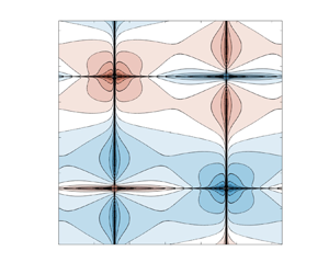



1. Introduction
We study the stability of a two-dimensional (2-D) flow of an incompressible ideal fluid described by the classical Euler system subject to periodic boundary conditions,
 $$\begin{align} {\partial_t \boldsymbol u} + (\boldsymbol u \boldsymbol{\cdot}\boldsymbol{\nabla})\boldsymbol u &={-} \boldsymbol{\nabla} p,\quad (\boldsymbol x, t) \in \mathbb{T}^2 \times (0, +\infty), \end{align}$$
 $$\begin{align}\boldsymbol{\nabla} \boldsymbol{\cdot} \boldsymbol u &= 0, \quad (\boldsymbol x, t) \in \mathbb{T}^2 \times (0, +\infty), \end{align}$$
 $$\begin{align}\boldsymbol u (\boldsymbol x, 0)&= \boldsymbol u_0(\boldsymbol{x}),\quad \boldsymbol x\in \mathbb{T}^2, \end{align}$$
where  $\mathbb {T}^2 := \mathbb {R}^2/ (2 {\rm \pi}\mathbb {Z})^2$ (‘
 $:=$’ means ‘equal to by definition’), whereas
 $\boldsymbol {x} = (x_1,x_2)^{\rm T}$ and
 $t \ge 0$ are respectively the spatial coordinate and time. In (1.1),
 $\boldsymbol u = \boldsymbol {u}(t, \boldsymbol {x}) = (u_1, u_2)^{\rm T}$ is the velocity field,
 $p = p (t, \boldsymbol x)$ the scalar pressure, whereas
 $\boldsymbol u_0$ is the initial condition for the velocity field, assumed divergence-free,
 $\boldsymbol {\nabla }\boldsymbol {\cdot } \boldsymbol u_0 = 0$.
Computing the curl of both sides of (1.1a), the equation for the scalar vorticity  ${\omega := \boldsymbol {\nabla }^\perp \boldsymbol {\cdot } \boldsymbol u}$, where
 ${\boldsymbol {\nabla }^\perp := (-\partial _{x_2},\partial _{x_1})}$, is
 $$\begin{align} \partial_t \omega + (\boldsymbol u \boldsymbol{\cdot}\boldsymbol{\nabla})\omega &= 0,\quad (\boldsymbol x, t) \in \mathbb{T}^2 \times (0, +\infty), \end{align}$$
 $$\begin{align}\boldsymbol u &= {\boldsymbol{\nabla}^\perp \varDelta^{{-}1} \omega},\quad (\boldsymbol x, t) \in \mathbb{T}^2 \times (0, +\infty), \end{align}$$
 $$\begin{align}\omega(\boldsymbol x, 0) &= \omega_0(\boldsymbol x),\quad \boldsymbol x \in \mathbb{T}^2, \end{align}$$
in which  ${\omega _0 := \boldsymbol {\nabla }^\perp \boldsymbol {\cdot } \boldsymbol u_0}$ and it will be assumed that
 $\int _{\mathbb {T}^2} \omega _0(\boldsymbol {x}) \,{\rm d}\kern0.07em\boldsymbol {x} = 0$ such that
 $\int _{\mathbb {T}^2} \omega (t,\boldsymbol {x}) \,{\rm d}\kern0.07em\boldsymbol {x} = 0$ for all
 $t> 0$. Hereafter, our focus will be on the vorticity formulation (1.2). We will refer to Sobolev spaces
 $H^m(\mathbb {T}^2)$,
 $m \in \mathbb {R}$, with the inner product defined as
 ${\langle\, f, g \rangle _{H^m} := \int _{\mathbb {T}^2} (1- \varDelta )^m \bar {f} g \,{\rm d}\kern0.07em\boldsymbol x}$, where
 $\bar {\cdot }$ denotes complex conjugation such that the norm is given by
 $\|\, f \|_{H^m} = \sqrt { \langle\, f, g \rangle _{H^m}}$ (Adams & Fournier Reference Adams and Fournier2005). Without loss of generality, we will focus our discussion on a subspace of
 $H^m(\mathbb {T}^2)$ consisting of zero-mean functions
 \begin{equation} {H^m_0(\mathbb{T}^2) := \left\{f\in H^m(\mathbb{T}^2), \int_{\mathbb{T}^2}f \,{\rm d}\kern0.07em\boldsymbol x = 0 \right\}.} \end{equation}
We will also use the space  $L^2(\mathbb {T}^2) := H^0(\mathbb {T}^2)$. In addition, we will consider Lebesgue and Sobolev non-inner-product spaces
 $L^p(\mathbb {T}^2)$ and
 $W^{1,p}(\mathbb {T}^2)$ with the norms
 $\|\, f \|_{L^p} := (\int _{\mathbb {T}^2} | f |^p \,{\rm d}\kern0.07em\boldsymbol {x})^{1/p}$ and
 $\|\,f \|_{W^{1,p}} := \|\,f \|_{L^p} + \| \boldsymbol {\nabla } f \|_{L^p}$ with
 $1 \le p < \infty$.
Analysis of the stability of equilibrium solutions  $\omega _s = \omega _s(\boldsymbol {x})$ of system (1.2) is a classical subject in mathematical fluid mechanics with general results describing conditions under which flows become unstable. The metric chosen to measure the deviation from the equilibrium captures different scales of instability – higher regularity spaces
 $H^m(\mathbb {T}^2)$ with
 $m > 0$ register finer structures, such as filamentation, while the energy space
 $H^{-1}(\mathbb {T}^2)$ captures large-scale instabilities. Koch's theorem (Koch Reference Koch2002) states that in the finer sense, i.e. if the evolution of the vorticity
 $\omega (t)$ is measured in the Hölder space
 $C^{k,\alpha }$, for any
 $k\in \mathbb {N}$ and
 $\alpha > 0$, any non-isochronous equilibrium in 2-D is nonlinearly Lyapunov unstable. Here, ‘non-isochronous’ means that all Lagrangian trajectories in the equilibrium flow do not have the same period (a typical example of an isochronous flow is solid-body rotation).
Most large-scale instabilities are classically attributed to laminar oscillatory structures as was established by the pioneering Rayleigh–Fjortoft–Tollmien inflection point theory and its contemporary operator theoretical formulations (Chandrasekhar Reference Chandrasekhar1961; Drazin & Reid Reference Drazin and Reid1981; Friedlander, Vishik & Yudovich Reference Friedlander, Vishik and Yudovich2000; Schmid & Henningson Reference Schmid and Henningson2001; Lin Reference Lin2005). In this case, instability arises from a smooth unstable mode of the linearized equation, which in turn gives rise to nonlinear instability in the energy space by the full analogue of the Lyapunov theorem, see Friedlander, Strauss & Vishik (Reference Friedlander, Strauss and Vishik1997), Lin (Reference Lin2004) and references therein. However, one of the simplest equilibrium solutions of (1.1)–(1.2) to which this theory does not apply is the 2-D Taylor–Green vortex, which is defined as
 \begin{equation} \boldsymbol u_s(\boldsymbol{x}) = (-\cos(x_1)\sin(x_2), \sin(x_1)\cos(x_2))^{\rm T},\quad \omega_s(\boldsymbol{x}) = 2\cos(x_1)\cos(x_2) \end{equation}
and features a doubly periodic array of cellular vortices. Some non-trivial generalizations of this equilibrium were recently considered by Zhigunov & Grigoriev (Reference Zhigunov and Grigoriev2023).
However, short-wavelength instabilities have been studied using an asymptotic Wentzel–Kramers–Brillouin (WKB) approach borrowed from geometric optics in which the solution of the linearization of (1.1) is represented as  $\boldsymbol {u}(t,\boldsymbol {x}) = \boldsymbol {a}(t,\boldsymbol {x},\boldsymbol {\xi }_0) \exp [ {\rm i} S(t,\boldsymbol {x},\boldsymbol {\xi }_0) / \delta ] + {O}(\delta )$ for some
 $\delta > 0$, where
 $\boldsymbol {\xi } := \boldsymbol {\nabla } S$ is the wavenumber of the perturbation and an analogous representation is used for the pressure
 $p(t,\boldsymbol {x})$ (Friedlander & Vishik Reference Friedlander and Vishik1991; Lifschitz & Hameiri Reference Lifschitz and Hameiri1991). Considering the leading-order expressions obtained by plugging these ansätze into the linearization of (1.1) and then taking the asymptotic limit
 $\delta \rightarrow 0$ followed by switching to the Lagrangian representation, one obtains a system of ordinary differential equations (ODEs) describing the evolution of the Lagrangian coordinate
 $\boldsymbol {x}(t;\boldsymbol {x}_0)$, the perturbation wavenumber
 $\boldsymbol {\xi }(t;\boldsymbol {x}_0,\boldsymbol {\xi }_0)$ and the amplitude of the perturbation
 $\boldsymbol {a}(t;\boldsymbol {x}_0,\boldsymbol {\xi }_0,\boldsymbol {a}_0)$ as a function of the corresponding initial conditions
 $\boldsymbol {x}_0$,
 $\boldsymbol {\xi }_0$ and
 $\boldsymbol {a}_0$ (chosen such that
 $\boldsymbol {\xi }_0 \boldsymbol {\cdot } \boldsymbol {a}_0 = 0$ to ensure incompressibility). This system of ODEs, referred to as the bicharacteristic problem, describes the time evolution of oscillatory perturbations in the short-wavelength limit. An instability of an equilibrium can then be detected if one can find a solution of this system such that
 $|\boldsymbol {a}(t;\boldsymbol {x}_0,\boldsymbol {\xi }_0,\boldsymbol {a}_0)|$ grows in time. While this approach makes it possible to conclude about an instability of the equilibrium, given its local Lagrangian nature, it does not provide any information about the global structure of the instability in space.
The 2-D Taylor–Green vortex (1.4a,b) is one of a number of exact solutions of the Euler equations known in a closed form. In the presence of viscosity  $\nu$, the velocity field (1.4a,b) gives rise to a closed-form solution of the Navier–Stokes system which decays in time as
 ${O}({\rm e}^{-\nu t})$. Therefore, the Taylor–Green vortex often serves as a benchmark in computational fluid dynamics. Most of the investigations of the stability of the 2-D Taylor–Green vortex have been carried out in the viscous setting where (1.4a,b) is not an exact equilibrium solution of the Navier–Stokes system. However, the main underlying assumption in these studies was that the time scale on which the instabilities develop is much shorter than
 ${O}({\rm e}^{-\nu t})$, the rate of the viscous decay of (1.4a,b). These investigations typically involved WKB analysis, solution of the eigenvalue problem for the linearized operator and/or time integration of the governing equations, all of which were performed numerically. They included analysis of elliptic instabilities under three-dimensional (3-D) perturbations (Sipp & Jacquin Reference Sipp and Jacquin1998; Kerswell Reference Kerswell2002; Aspden & Vanneste Reference Aspden and Vanneste2009) and hyperbolic instabilities (Friedlander & Vishik Reference Friedlander and Vishik1991; Leblanc & Godeferd Reference Leblanc and Godeferd1999; Suzuki, Hirota & Hattori Reference Suzuki, Hirota and Hattori2018). A thorough discussion of different instability mechanisms possible in the Taylor–Green vortex under rotation and/or stratification can be found from Hattori & Hirota (Reference Hattori and Hirota2023). The elliptic instability is closely related to elliptic stagnation points in the base flow and only occurs when the perturbation is 3-D, crucially depending on the wavenumber of the perturbation along the direction orthogonal to the plane of motion. On the other hand, the hyperbolic instability is connected to hyperbolic stagnation points and appears even under 2-D perturbations (Gau & Hattori Reference Gau and Hattori2014), which is more relevant to the current study where we focus on analysing the stability of 2-D flows. In particular, in this latter study, the authors considered a problem similar to that investigated here. However, as will be evident below, our findings are in fact quite different, underlining the difference between the viscous and inviscid formulations.
In contrast to these earlier studies, our focus here is on the instability of the Taylor–Green vortex (1.4a,b) in 2-D inviscid Euler flows governed by (1.1)–(1.2). Even though, at a formal level, the Euler equations under periodic boundary conditions can be viewed as the vanishing viscosity limit of the Navier–Stokes equations, the spectra of the corresponding linearized operators are fundamentally different. Unlike the linearized Navier–Stokes operator, the linearized Euler operator is not elliptic, thus the existent theory about elliptic operators cannot be applied. Moreover, it is also degenerate and non-self-adjoint, which further complicates the analysis. Most importantly, the spectrum of the linearized Navier–Stokes operator defined on a bounded domain subject to Dirichlet boundary conditions or periodic boundary conditions can only consist of the discrete spectrum and the corresponding eigenfunctions are smooth. Shvydkoy & Friedlander (Reference Shvydkoy and Friedlander2008) proved that the eigenvalues of the linearized Navier–Stokes operator converge to unstable eigenvalues of the linearized Euler operator which are outside the essential spectrum as viscosity goes to zero, if such eigenvalues exist. However, despite the simple structure of the 2-D Taylor–Green vortex (1.4a,b), the existence of unstable eigenvalues of the corresponding linearized Euler operator is still an open question. If such unstable eigenvalues exist, the regularity of the corresponding eigenfunctions is not a priori known and may be determined by the location of these eigenvalues relative to the essential spectrum (Lin Reference Lin2005). Thus, due to these nuances, the inviscid problem is distinct from its viscous counterpart.
Since the spectra of the linearized Euler operators obtained by linearizing the velocity formulation (1.1) and the vorticity formulation (1.2) are equivalent (Shvydkoy & Latushkin Reference Shvydkoy and Latushkin2005), in this study, we use the latter formulation and provide numerical evidence that the linearized operator has unstable eigenvalues approximately equal to  $0.1424 \pm 0.5875 i$ with the corresponding eigenfunctions given by distributions in
 $H^{0.28}_0(\mathbb {T}^2)$, where the level of regularity
 $s = 0.28$ is determined approximately based on Lin's theorem (Lin Reference Lin2004), as will be discussed in § 2. This eigenfunction exhibits a more regular profile in the laminar cells loosing its smoothness in the vicinity of the heteroclinic orbits of the equilibrium (1.4a,b). We also illustrate another distinct instability mechanism associated with a continuous family of uncorrelated functions corresponding to points in the essential spectrum, which is quite different from the modal growth observed in the former case. Since the essential spectrum does not arise in a finite-dimensional setting, investigation of these questions requires the use of computational tools which are more refined as compared with the techniques typically employed in the studies of hydrodynamic stability (Schmid & Henningson Reference Schmid and Henningson2001). Obtaining these results is enabled by the solution of a suitably defined partial differential equation (PDE) optimization problem. Such optimization-based formulations have had a long history in the study of flow stability problems, both linear and nonlinear (Schmid & Henningson Reference Schmid and Henningson2001; Kerswell, Pringle & Willis Reference Kerswell, Pringle and Willis2014; Kerswell Reference Kerswell2018). However, given the subtle infinite-dimensional nature of the optimization problem considered here, we solve it using a specialized variant of the adjoint-based approach which allows us to impose different levels of regularity on the obtained optimal initial conditions (Zhao & Protas Reference Zhao and Protas2023). By solving this optimization problem using increasing spatial resolutions, we obtain a sequence of functions that are localized near the hyperbolic stagnation points of the equilibrium solution (1.4a,b) and reveal high-frequency oscillations restricted by the spatial resolution. Importantly, using these functions as initial conditions, the corresponding solutions of the linearized Euler system reveal growth rates saturating rigorous a priori bounds on the growth of the semigroup induced by the essential spectrum of the generator. While these results are consistent with the findings of the WKB analysis, they also provide information about the global spatial structure of the perturbations realizing this maximum possible growth.
The structure of the paper is as follows: in § 2, we introduce the problems of linear and nonlinear instability and discuss the spectrum of the linearized Euler operator; in § 3, we discuss the numerical discretization of the linearized operator to compute its eigenvalues as well as the formulation of a PDE optimization problem to obtain initial conditions such that the corresponding flows realize the largest growth rate of perturbations predicted by the form of the essential spectrum, which is solved using a Riemannian conjugate gradient method described in Appendix A; in § 4, we illustrate two distinct mechanisms that lead to a linear instability – a modal growth and a non-modal growth of the solution, where the former corresponds to the point spectrum, while the latter corresponds to the essential spectrum of the linearized operator and is highly dependent on the function space in which the perturbation is defined. Additionally in that section, we discuss some computational results concerning the nonlinear instability. A discussion and final conclusions are deferred to § 5.
2. Linear and nonlinear stability
Linearizing system (1.2) around a steady solution  $\{\boldsymbol u_s, \omega _s\}$, we obtain the following system:
 $$\begin{align} \partial_t w &= \mathcal{L} w,\quad (\boldsymbol x, t) \in \mathbb{T}^2 \times (0, +\infty), \end{align}$$
 $$\begin{align}w(\boldsymbol x, 0) &= w_0(\boldsymbol x),\quad \boldsymbol x \in \mathbb{T}^2, \end{align}$$
where the linearized Euler operator  $\mathcal {L}$ is given by
 \begin{equation} \mathcal{L} w :={-}(\boldsymbol u_s\boldsymbol{\cdot}\boldsymbol{\nabla}) w -({\boldsymbol u} \boldsymbol{\cdot}\boldsymbol{\nabla})\omega_s = {[ -\boldsymbol u_s \boldsymbol{\cdot}\boldsymbol{\nabla} - \boldsymbol{\nabla}\omega_s\boldsymbol{\cdot} (\boldsymbol{\nabla}^\perp \varDelta^{{-}1})] w}. \end{equation}
The solution of system (2.1) can be written as  $w(t) = {\rm e}^{t \mathcal {L}} w_0$, where
 $w(t) := w(t,{\cdot })$ and
 ${\rm e}^{t \mathcal {L}}$ is the semigroup induced by the operator
 $\mathcal {L}$ (Engel & Nagel Reference Engel and Nagel2000). The question of stability of the equilibrium
 $\omega _s$ is thus linked to the asymptotic, as
 $t \rightarrow \infty$, behaviour of
 $\| {\rm e}^{t \mathcal {L}} \|_{H^m}$ quantified by the growth abscissa
 $\gamma (\mathcal {L}) := \lim _{t \rightarrow \infty } t^{-1} \ln \| {\rm e}^{t \mathcal {L}} \|_{H^m}$, which is in turn determined by the spectrum
 $\sigma (\mathcal {L})$ of the operator
 $\mathcal {L}$. While in finite dimensions it is determined by the eigenvalue with the largest real part, in infinite dimensions, the situation is more nuanced since there exist operators
 $\mathcal {A}$ such that
 $\sup _{z \in \sigma (\mathcal {A})} {\rm Re}(z) < \gamma (\mathcal {A})$, e.g. Zabczyk's problem (Zabczyk Reference Zabczyk1975; Trefethen Reference Trefethen1997); some problems in hydrodynamic stability where such behaviour was identified are analysed by Renardy (Reference Renardy1994).
Following Browder (Reference Browder1961), we decompose the spectrum of  $\mathcal {L}$ into two disjoint sets: the discrete spectrum and the essential spectrum, as follows:
 \begin{equation} \sigma(\mathcal{L}) = \sigma_{{\text{disc}}}(\mathcal{L}) \cup \sigma_{{\text{ess}}}(\mathcal{L}). \end{equation}
We then say that  $z \in \sigma _{\text {disc}}(\mathcal {L})$ if it satisfies the following conditions:
(i)
 $z$ is an isolated point in $\sigma (\mathcal {L})$;
(ii)
$z$ has finite multiplicity, i.e. $\bigcup _{r=1}^\infty \mathrm {Ker}(z - \mathcal {L})^r$ is finite dimensional;(iii) the range of
$z-\mathcal {L}$ is closed.


Otherwise,  $z$ is called a point of the essential spectrum
 $\sigma _{ess}(\mathcal {L})$. To illustrate this concept, we consider the linear operator
 $T$ that maps all functions in
 $L^2_0(\mathbb {T})$ to the zero function. It has only the essential spectrum
 $\sigma _{\text {ess}}(T) = \{0\}$ as its kernel
 $\mathrm {Ker}(T) = L^2_0(\mathbb {T})$ is infinite-dimensional. As a more complicated example, we consider the linear operator
 $T: L^2_0(\mathbb {T}) \to L^2_0(\mathbb {T})$ defined by
 \begin{equation} T[f](x) := \sum_{n=1}^\infty \frac{1}{n}(a_n\cos(nx) + b_n\sin(nx)),\quad \text{where}\ f(x) = \sum_{n=1}^\infty (a_n\cos(nx) + b_n\sin(nx)). \end{equation}
For any positive integer  $p$,
 $1/p$ is an eigenvalue of
 $T$, and
 $\cos (p x)$ and
 $\sin (p x)$ are the corresponding eigenfunctions. Since
 $T$ is not surjective,
 $0 \in \sigma (T)$ and since
 $\lim _{p\to \infty } (1/p) = 0$, 0 is not an isolated point in the spectrum of
 $T$. Therefore, we have
 $\sigma _{{\text {disc}}}(T) = \{1/p,\ p \in \mathbb {N}_+\}$ and
 $\sigma _{{\text {ess}}}(T) = \{0\}$.
While in finite dimensions linear operators can be represented as matrices which can only have a discrete spectrum, in infinite dimensions, the situation is complicated by the presence of the essential spectrum. We refer to the set of eigenvalues of  $\mathcal {L}$ as the point spectrum
 \begin{equation} {\sigma_{p}(\mathcal{L}) := \{\lambda \in \mathbb{C}: \exists \phi (\boldsymbol{x}) \neq 0, \mathcal{L} \phi (\boldsymbol{x}) = \lambda \phi (\boldsymbol{x}),\ \boldsymbol{x} \in \mathbb{T}^2\}}, \end{equation}
where  $\phi$ is the eigenfunction corresponding to the eigenvalue
 $\lambda$. It follows from the discrete translation symmetry of the 2-D Taylor–Green vortex (1.4a,b) and the continuous translation invariance of the Euler system (1.1) that if
 $\phi (x_1, x_2)$ is an eigenfunction corresponding to
 $\lambda$, then so is
 $\phi (-x_1, -x_2)$, whereas
 $\phi (x_1+{\rm \pi}, x_2)$,
 $\phi (x_1, x_2+{\rm \pi} )$,
 $\phi (-x_1, x_2)$ and
 $\phi (x_1, -x_2)$ are eigenfunctions corresponding to
 $-\lambda$.
As regards the discrete spectrum  ${\sigma _{\text {disc}}}(\mathcal {L})$ of the linearized Euler operator (2.1), some results are available only for certain flows such as parallel and rotating shear flows (Chandrasekhar Reference Chandrasekhar1961; Drazin & Reid Reference Drazin and Reid1981; Friedlander et al. Reference Friedlander, Strauss and Vishik1997) and the cellular ‘cat's-eye’ flow (Friedlander et al. Reference Friedlander, Vishik and Yudovich2000). In the absence of general results, one of the goals of the present study is to consider this question in the context of the Taylor–Green vortex (1.4a,b). Unlike the aforementioned two cases, where the instability is closely related to the shear flow structure of the equilibria, equilibrium (1.4a,b) possesses a cellular structure only.
On the other hand, the essential spectrum  $\sigma _{ess}(\mathcal {L})$ of the linear operator
 $\mathcal {L}$ is fully understood (Shvydkoy & Latushkin Reference Shvydkoy and Latushkin2003): in
 $H^{m}_0(\mathbb {T}^2)$,
 $m \in \mathbb {R}$, it is given by the strip
 \begin{equation} \sigma_{ess}(\mathcal{L}; H^{m}_0) = \{ z\in \mathbb{C}: |{{\rm Re}}(z)| \leq |m| \, \mu_{max}\}, \end{equation}
where  $\mu _{max}$ is the maximal Lyapunov exponent corresponding to the Lagrangian flow
 $\varphi _t: \boldsymbol {\xi } \to \boldsymbol x(t; \boldsymbol {\xi })$ generated by the steady state via
 $\partial _t \boldsymbol x(t) = \boldsymbol u_s (\boldsymbol x(t))$,
 \begin{equation} {\mu_{max}} = \lim_{t\to\infty} \frac{1}{t}\log \sup_{\boldsymbol x\in\mathbb{T}^2} ||\boldsymbol{\nabla}\varphi_t(\boldsymbol x)||. \end{equation}
In 2-D,  $\mu _{max}$ can only be attained at a hyperbolic stagnation point
 $\boldsymbol {x}_s$ of the flow
 $\{\varphi _t\}$ induced by the steady state
 $\boldsymbol {u}_s$ and is determined by the largest real part of the eigenvalues of the velocity gradient
 $\boldsymbol {\nabla }\boldsymbol {u}_s({\boldsymbol {x}_s})$ evaluated over all stagnation points
 ${\boldsymbol {x}_s}$ (Shvydkoy & Friedlander Reference Shvydkoy and Friedlander2005). The equilibrium state (1.4a,b) has four hyperbolic stagnation points
 $\boldsymbol {x}_s = \{({\rm \pi} /2, {\rm \pi}/2), ({\rm \pi} /2, 3{\rm \pi} /2), (3{\rm \pi} /2, {\rm \pi}/2), (3{\rm \pi} /2, 3{\rm \pi} /2)\}$. By computing the eigenvalues of
 $\boldsymbol {\nabla } \boldsymbol {u}_s$ at these four points, we deduce that
 ${\mu _{max}} = 1$. Another interesting property of the stagnation points is that the action of the linearized operator on any sufficiently smooth function
 $w$ vanishes at these points, i.e.
 \begin{align} \mathcal{L} w = 0 \quad \text{at}\ \boldsymbol{x} = \boldsymbol{x}_s. \end{align}
At the same time, we also have
 \begin{equation} \sigma({\rm e}^{t\mathcal{L}}; H^{m}) = \{ z \in \mathbb{C}: \exp({-t|m|}) \leq |z| \leq \exp({t|m|})\}, \end{equation}
such that the full analogue of the spectral mapping theorem holds (Shvydkoy & Latushkin Reference Shvydkoy and Latushkin2003). All points in the band and the annulus are points of the essential spectrum in the Browder sense (Browder Reference Browder1961), which is the broadest definition of the essential spectrum also coinciding with the Fredholm spectrum. In the proof, for any point  $z\in \sigma _{ess}(\mathcal {L})$, Shvydkoy & Latushkin (Reference Shvydkoy and Latushkin2003) constructed approximate eigenfunctions as a sequence of unit vectors
 $\{f_n\} \in H^m_0(\mathbb {T}^2)$ such that
 $\|(\mathcal {L} - z) f_n \|_{H^m} \rightarrow 0$ as
 $n \rightarrow \infty$, and
 $\{f_n\}$ does not contain any convergent subsequence. These approximate eigenfunctions are characterized by highly oscillatory behaviour and are stretched along the heteroclinic orbits of
 $\boldsymbol u_s$ while concentrating towards the hyperbolic points. These results are consistent with the asymptotic WKB analysis conducted in the neighbourhood of the hyperbolic stagnation points which suggests the presence of highly oscillatory perturbations growing as
 ${O}({\rm e}^{\mu _{max} t})$, though they need not be eigenfunctions of
 $\mathcal {L}$ (Friedlander & Vishik Reference Friedlander and Vishik1991; Lifschitz & Hameiri Reference Lifschitz and Hameiri1991). In general, it is unknown whether the operator
 $\mathcal {L}$ has any unstable eigenvalues. However, when it does, the regularity of the corresponding eigenfunctions is characterized by a theorem of Lin (Reference Lin2004) which we state here in a slightly less general version adapted to the case when the equilibrium is given by the Taylor–Green vortex (1.4a,b).
Theorem 2.1 (Lin Reference Lin2004)
Suppose there exists an exponentially growing solution  ${\rm e}^{\lambda t} w_0$ of the linearized system
 $\partial _t w = \mathcal {L} w$ with
 ${\rm Re}(\lambda ) > 0$ and let
 $w_0 \in L^2(\mathbb {T}^2)$. Then, we have the following:
(i) [regularity of growing modes]
$w_0 \in W^{1,p}(\mathbb {T}^2) \cap L^q(\mathbb {T}^2)$ for all $1 \le p < p^*$ and $1 \le q < \infty$, where
(2.10)\begin{equation} p^* = \begin{cases} \dfrac{\mu_{max}}{\mu_{max} - {\rm Re}(\lambda)} = \dfrac{1}{1 -{\rm Re}(\lambda)}, & \mu_{max} > {\rm Re}(\lambda), \\ \infty, & \mu_{max} \le {\rm Re}(\lambda); \end{cases} \end{equation}(ii) [nonlinear instability] for any
$p \in [1,p^*)$, $q\in [1,\infty )$, $m\in [-1,\infty )$, there exists $\epsilon > 0$, such that for any $\delta > 0$, there is a solution $\omega ^\delta (t)$ of the 2-D Euler system (1.2) corresponding to the initial condition $\omega _0^{\delta }$, satisfying
(2.11)and\begin{equation} \| \omega_0^{\delta} - \omega_s\|_{L^q} + \| \boldsymbol{\nabla}(\omega_0^{\delta} - \omega_s)\|_{L^p} \le \delta, \end{equation}(2.12)\begin{equation} \sup_{0 < t < T_\delta} \|\omega^\delta(t) - \omega_s\|_{H^m} \geq \epsilon. \end{equation}


While for general infinite-dimensional nonlinear systems linear instability need not imply a nonlinear instability, the second part of the theorem above asserts that this is in fact the case for the 2-D Euler problem, provided the unstable eigenfunction of the linearized operator  $\mathcal {L}$ is sufficiently regular.
As a key result of the present study, we provide numerical evidence that the operator  $\mathcal {L}$ does possess unstable eigenvalues and we also characterize the regularity of the corresponding eigenfunctions concluding that it is consistent with Theorem 2.1, part (i), cf. § 4.1.1. The nonlinear instability predicted in part (ii) of the theorem is illustrated in § 4.2. Another contribution of the present study is to illustrate the non-trivial instability mechanism associated with the unstable essential spectrum, cf. § 4.1.2.
3. Numerical approaches
In this section, we introduce the numerical approaches that will allow us to characterize the growth of solutions of the linear and nonlinear problems (2.1) and (1.2). First, in § 3.1, we describe a numerical solution of the eigenvalue problem (2.5) such that the eigenfunctions  $\phi$ corresponding to the eigenvalues
 $\lambda \in \sigma _{p}(\mathcal {L})$ can be used as the initial condition in the linear and nonlinear problems (2.1) and (1.2) (in the latter case, the eigenfunctions serve as perturbations of the equilibrium (1.4a,b)). Then, in § 3.2, we introduce an optimization-based approach allowing us to construct solutions of the linear problem (2.1) saturating the spectral bounds (2.6) and (2.9). Finally, in § 3.3, we describe the approach to the numerical solution of the evolutionary systems (1.2), (2.1) and its adjoint.
3.1. The point spectrum of the linear operator $\mathcal {L}$

To characterize the point spectrum  ${\sigma _{p}(\mathcal {L})}$, we adopt a Galerkin approach where the operator
 $\mathcal {L}$ is discretized using the following orthonormal basis in
 ${H^m_0(\mathbb {T}^2)}$:
 $$\begin{align} \varphi_{j_1, j_2}(\boldsymbol{x}) &:= \frac{1}{\sqrt{2}{\rm \pi}} (1 + j_1^2 + j_2^2)^{{-}m/2}\cos(j_1 x_1 + j_2 x_2),\\ &\quad j_1, j_2 \in \mathbb{N}, \nonumber\end{align}$$
 $$\begin{align}\psi_{j_1, j_2}(\boldsymbol{x}) &:={-}\frac{1}{\sqrt{2}{\rm \pi}} (1 + j_1^2 + j_2^2)^{{-}m/2} \sin(j_1 x_1 + j_2 x_2), \end{align}$$
and we have
 \begin{equation} \left.\begin{gathered}
\mathcal{L} \varphi_{j_1,j_2} = \alpha (\varphi_{j_1+1,
j_2+1} - \varphi_{j_1-1, j_2-1}) + \beta (-\varphi_{j_1+1,
j_2-1} + \varphi_{j_1-1, j_2+1}), \\ \mathcal{L}
\psi_{j_1,j_2} = \alpha (\psi_{j_1+1, j_2+1} - \psi_{j_1-1,
j_2-1}) + \beta (-\psi_{j_1+1, j_2-1} + \psi_{j_1-1,
j_2+1}),\\ \text{where}\quad \alpha =
\frac{(j_1-j_2)(j_1^2+j_2^2-2)}{4(j_1^2+j_2^2)},\quad \beta
= \frac{(j_1+j_2)(j_1^2+j_2^2-2)}{4(j_1^2+j_2^2)}.
\end{gathered}\right\}
\end{equation}
In the computations, we approximate functions in  $H^m_0(\mathbb {T}^2)$ using a finite subset of the basis (3.1),
 \begin{equation} \mathcal{W}^N = \{\varphi_{0, j_2}, \psi_{0, j_2}: 1\leq j_2 \leq N\} \bigcup \{\varphi_{j_1, j_2}, \psi_{j_1, j_2}: 1\leq j_1 \leq N, -N\leq j_2\leq N\}, \end{equation}
which contains  $|\mathcal {W}^N| = 2\sum _{s = 1}^N 4s = 4N(N+1)$ elements. We label the basis functions in
 $\mathcal {W}^N$ using the ‘spiral’ ordering, i.e.
 \begin{equation} \left.\begin{gathered}
\begin{aligned} p_{n+2j} &= \varphi_{j, s},& p_{n+2j+1}
&= \psi_{j, s}, \\ p_{n+2s+2j} &= \varphi_{s, s-j},&
p_{n+2s+2j+1} &= \psi_{s, s-j},\\ p_{n+4s+2j} &= \varphi_{s,
-j},& p_{n+4s+2j+1} &= \psi_{s, -j}, \\ p_{n+6s+2j} &=
\varphi_{s-j, 1-s},& p_{n+6s+2j+1} &= \psi_{s-j, 1-s},
\end{aligned}\quad \begin{gathered} n = 1+4s(s-1), \\
0\leq j\leq s-1,\quad 1\leq s \leq N. \end{gathered}
\end{gathered}\right\}
\end{equation}
Given a function  $f \in H_0^m(\mathbb {T}^2)$, we thus define its Galerkin approximation
 $f^N$ by
 \begin{equation} f \approx f^N := \sum_{j = 1}^{|\mathcal{W}^N|} \hat{f}_j p_j,\quad \hat{f}_j = \langle\, f, p_j \rangle_{H^m}. \end{equation}
Approximating the eigenfunctions  $\phi$ in (2.5) in terms of the truncated Fourier series (3.5), we arrive at the discrete algebraic eigenvalue problem
 \begin{equation} \boldsymbol{L} \phi = \lambda \phi, \end{equation}
where  $\boldsymbol {L}$ is a
 ${|\mathcal {W}^N|\times |\mathcal {W}^N|}$ matrix whose entries are determined by relations (3.2) as
 \begin{equation} \boldsymbol{L}_{j,k} = \langle \mathcal{L} p_k,\ p_j\rangle_{H^m},\quad 1 \leq j, k \leq {|\mathcal{W}^N|}. \end{equation}
As a result of relations (3.2), matrix  $\boldsymbol {L}$ is sparse, with at most four non-zero entries in each row and column. Moreover, since
 \begin{align} \langle \mathcal{L} p_k,\ p_j\rangle_{H^m} &= {\langle (1-\varDelta^{{-}1})^{m/2}\mathcal{L} p_k, (1-\varDelta^{{-}1})^{m/2}p_j\rangle_{L^2}} \nonumber\\ &= {\langle [(1-\varDelta^{{-}1})^{m/2}\mathcal{L}(1-\varDelta^{{-}1})^{{-}m/2}] (1-\varDelta^{{-}1})^{m/2} p_k,\ (1-\varDelta^{{-}1})^{m/2} p_j\rangle_{L^2},} \end{align}
the matrices  $\boldsymbol {L}$ computed in different Sobolev spaces
 $H_0^m(\mathbb {T}^2)$ are similar. Therefore, without loss of generality, we can focus our discussion on the matrix constructed with
 $m = 0$, i.e. in
 $L^2_0(\mathbb {T}^2)$.
We adopt two different methods to numerically solve the algebraic eigenvalue problem (3.6). As the first method, we use the eigenvalue solver dgeev from the LAPACK library to compute all eigenvalues of  $\boldsymbol {L}$. This approach provides a complete picture of the spectrum of the matrix
 $\boldsymbol {L}$, but is computationally expensive, limiting the resolution to
 $N^2 = 200^2$. The second method takes advantage of the sparse structure of the matrix
 $\boldsymbol {L}$ and uses a Krylov subspace method (Hattori & Hirota Reference Hattori and Hirota2023) to only compute the eigenvalue with the largest real part and the corresponding eigenvector. Specifically, we use the Matlab function eigs, setting the dimension of the Krylov subspace to 20, the tolerance to
 $10^{-10}$ and the maximum number of iterations to 1000. To validate these results, at
 $N^2 = 200^2$, we use a random vector to generate the Krylov subspace, and the obtained eigenvalues with the largest real part are found to be essentially the same as those obtained using the LAPACK subroutine dgeev. To speed up the computation, at the resolution
 $(2N)^2$, we use
 $\lambda _+^N$ as the shift and the corresponding eigenfunction
 $\phi _+^N$ as the generator of the Krylov subspace. This allows us to increase the numerical resolution from
 $N^2 = 200^2$ to
 $3000^2$. A combination of these two approaches makes it possible to obtain a global picture of the spectrum of the matrix
 $\boldsymbol {L}$, while also refining the approximations of the most interesting eigenvalues.
As is shown in § 4.1, employing the procedure described above, we obtain unstable eigenvalues whose real part is approximately 0.1424 and the corresponding eigenfunctions belong to  $H^{0.28}_0(\mathbb {T}^2) \subset L^2_0(\mathbb {T}^2)$. Using the real part of this eigenfunction as the initial condition in the linearized Euler equations (2.1), we observe an exponential growth of the
 $L^2$ norm of the solution
 $w(t)$ with the rate predicted by the real part of the unstable eigenvalue. However, as is evident from (2.6), in the Sobolev spaces
 $H^1$ and
 $H^{-1}$,
 $\sigma _{ess}(\mathcal {L})$ forms a vertical band
 $|{\textrm {Re}}(z)| \le 1$. It is thus a natural question what initial condition can realize the growth abscissa
 $\gamma (\mathcal {L}) = 1$ predicted by
 $\sigma _{ess}(\mathcal {L})$, which is larger than the growth rate realized by the unstable eigenfunction. Tools needed to address this question are discussed next.
3.2. The essential spectrum of the linear operator $\mathcal {L}$

As will be evident in § 4.1, the real part of the unstable eigenvalues of problem (2.5) found as described in § 3.1 is near 0.1424, and therefore, for  $m \neq 0$, does not saturate the bounds on the growth of the abscissa implied by (2.9). It is therefore natural to ask the question whether there exists an initial condition
 $w_0$ such that the growth rate of
 $||\textrm {e}^{t\mathcal {L}} w_0||_{H^m}$, i.e.
 $(\textrm {d}/\textrm {d} t) \ln (\| \textrm {e}^{t\mathcal {L}} w_0 \|_{H^{m}})$, saturates this bound. Since the essential spectrum is an inherently infinite-dimensional object, information about it is lost in a finite-dimensional truncation such as (3.5). We thus need an approach different from the method described in § 3.1 to study properties related to the essential spectrum. Instead of maximizing the growth rate of the solutions of (2.1) directly, we aim to maximize the norm of the solution
 $||\textrm {e}^{t\mathcal {L}} w_0||_{H^m}$ at some finite time
 $t = T > 0$ over all
 $w_0 \in H^m_0(\mathbb {T}^2)$. Since
 $\textrm {e}^{t \mathcal {L}} w_0$ is linear with respect to
 $w_0$, we can fix
 $\|w_0\|_{H^m} = 1$ without loss of generality. Therefore, we define the following objective functional
 $J: {H_0^m(\mathbb {T}^2)} \rightarrow \mathbb {R}$
 \begin{equation} J (w_0) = ||{\rm e}^{T\mathcal{L}} w_0||^2_{H^m},\end{equation}
and the corresponding optimization problem.
Problem 3.1 For  $T > 0$, find
 \begin{equation} {\tilde{w}_0 = \operatorname{argmax}_{w_0 \in \mathcal{M}} J (w_0),\quad \mathcal{M} := \{w_0 \in H^m_0(\mathbb{T}^2): \|w_0\|_{H^m} = 1\}.} \end{equation}
To observe a significant exponential growth of  ${||\textrm {e}^{T\mathcal {L}} w_0||_{H^m}}$, one normally chooses
 $T > O(\ln (\|w_0\|_{H^m}))$, and in our study, we use
 $T = 1$. Problem 3.1 has the form of a quadratically constrained quadratic program defined in terms of positive-semidefinite operators and is therefore convex.
While discretized versions of Problem 3.1 can in principle be solved by performing a singular-value decomposition of the corresponding matrix exponential (Schmid & Henningson Reference Schmid and Henningson2001), this is problematic when one has to ensure the required regularity of the optimal initial condition  $\tilde {w}_0$, which is encoded here in the choice of
 $m$. We therefore solve this problem using a Riemannian conjugate gradient method (Absil, Mahony & Sepulchre Reference Absil, Mahony and Sepulchre2008; Danaila & Protas Reference Danaila and Protas2017; Sato Reference Sato2021; Zhao & Protas Reference Zhao and Protas2023) which requires computation of the Sobolev gradient of
 ${J(w_0)}$, denoted
 ${\boldsymbol {\nabla } J(w_0)}$. Evaluating the Gâteaux (directional) differential
 ${J'(w_0; w_0'): H_0^m \times H^m_0 \to \mathbb {R}}$, which represents the variation of the objective function
 ${J(w_0)}$ in the direction of
 ${w'_0}$ at the point
 ${w_0}$, we obtain
 \begin{align} J'(w_0; w_0') &= \lim_{\epsilon \to 0} \frac{1}{\epsilon} [J(w_0 + \epsilon w_0') - J(w_0)] \nonumber\\ &= 2 \langle {\rm e}^{T\mathcal{L}} w_0,\ {\rm e}^{T\mathcal{L}} w_0'\rangle_{H^m} \nonumber\\ &= {2 \langle (1-\varDelta^{{-}1})^m \,{\rm e}^{T\mathcal{L}} w_0,\ {\rm e}^{T\mathcal{L}} w_0' \rangle_{L^2}} \nonumber\\ &= {2 \langle {\rm e}^{T\mathcal{L}^*} (1-\varDelta^{{-}1})^m \,{\rm e}^{T\mathcal{L}} w_0,\ w_0' \rangle_{L^2}} \nonumber\\ &= {2 \langle (1-\varDelta^{{-}1})^{{-}m} \,{\rm e}^{T\mathcal{L}^*} (1-\varDelta^{{-}1})^m \,{\rm e}^{T\mathcal{L}} w_0,\ w_0' \rangle_{H^m},} \end{align}
where  $\mathcal {L}^*$ is the adjoint of the linear operator
 $\mathcal {L}$ defined with respect to the
 $L^2$ inner product as
 $\langle \mathcal {L} f, g \rangle _{L^2} =\langle\, f, \mathcal {L}^*g \rangle _{L^2}$ and having the form
 \begin{equation} {\mathcal{L}^* = \boldsymbol{u}_s\boldsymbol{\cdot}\boldsymbol{\nabla} + \varDelta^{{-}1}(\boldsymbol{\nabla} w_s \boldsymbol{\cdot} \boldsymbol{\nabla}^\perp).} \end{equation}
Finally, using relation (3.11) and the Riesz representation theorem, the Sobolev gradient of  ${J(w_0)}$ with respect to the
 $H^m$ inner product is obtained as
 \begin{equation} {\boldsymbol{\nabla} J(w_0) = 2 (1-\varDelta^{{-}1})^{{-}m} \,{\rm e}^{T\mathcal{L}^*} (1-\varDelta^{{-}1})^m \,{\rm e}^{T\mathcal{L}} w_0.} \end{equation}
Details of the Riemannian conjugate gradient method we use to solve Problem 3.1 are described in Appendix A.
3.3. Numerical solution of the evolution problems
Here, we describe the numerical approach we use to solve the evolution problems (1.2), (2.1) and the adjoint problem defined in (3.12). We employ a standard Fourier–Galerkin pseudospectral method (Canuto et al. Reference Canuto, Hussaini, Quarteroni and Zang1988) where the solution is approximated in terms of a truncated Fourier series with the nonlinear term and the terms with non-constant coefficients evaluated in the physical space. In lieu of dealiasing, we use the Gaussian filter proposed by Hou & Li (Reference Hou and Li2007). The resulting system of ordinary differential equations is integrated in time using the RK4 technique and a massively parallel implementation based on MPI. Since the considered initial conditions are distributions, rather than smooth functions, cf. figure 2, the numerical solutions of problems (1.2) and (2.1) are not well resolved regardless of the resolution  $N^2$. However, the Galerkin projection implied by the truncation of the series, as in (3.5) together with the resolution-dependent filter, can be regarded as a regularization of the problem whose effect vanishes as the resolution is refined, i.e. as
 $N \rightarrow \infty$.
4. Results
Here, we describe the mechanisms of the linear growth of perturbations in the modal regime, associated with eigenvalues in the point spectrum  $\sigma _{p}(\mathcal {L})$, and in the non-modal regime, associated with points in the essential spectrum
 $\sigma _{ess}(\mathcal {L})$ that do not coincide with the point spectrum
 ${\sigma _{p}(\mathcal {L})}$. This is followed by a discussion of the growth of perturbations in the nonlinear regime. Hereafter, we will use the convention that the superscript
 $N$ will represent the resolution with which a given quantity, such as an eigenvalue, eigenfunction or a solution of the linear problem (2.1), is approximated.
4.1. Linear instability
As discussed in § 3.1, since in the discrete eigenvalue problem (3.6) the matrices corresponding to different values of  $m$ are similar, it suffices to solve the eigenvalue problem using
 $m = 0$ only. Figure 1(a) shows the eigenvalues of the discrete eigenvalue problem (3.6) with
 $m = 0$ obtained using the resolution
 $N^2 = 200^2$. We see that there are two pairs of conjugate eigenvalues
 ${\pm }\lambda _+^{200}, \overline {{\pm }\lambda _+^{200}}$, where
 $\lambda _+^{200}$ denotes the eigenvalue whose real and imaginary parts are both positive. To better resolve these eigenvalues and the corresponding eigenvectors, the discrete eigenvalue problem (3.6) is then solved with the Krylov method described in § 3.1 which leverages the sparsity of the matrix
 $\boldsymbol {L}$. This allows us to refine the resolution as
 $N^2 = 200^2, 400^2, \ldots 3000^2$ and the obtained eigenvalues
 $\lambda _+^N$ are shown in figure 1(b). We see that as the resolution
 ${N^2}$ increases, these eigenvalues converge to a well-defined limit; this limit is interpreted as the ‘true’ eigenvalue in the point spectrum
 ${\sigma _{p}(\mathcal {L})}$ (Boyd Reference Boyd2001). We denote
 $\lim _{N\to \infty } \lambda _+^N =: \lambda _+$ and at the largest resolution
 $N^2 = 3000^2$ have
 $\lambda _+^{3000} = 0.1424 + 0.5875i$, which is a numerical approximation of the ‘true’ unstable eigenvalue
 $\lambda _+$. We note that 0 is also an eigenvalue. On the other hand, all remaining eigenvalues of the discretized problem (3.6) fall on the imaginary axis and, as is evident from figures 1(b) and 1(c), they do not converge to well-defined limits. Instead, as the resolution
 $N^2$ is refined, the purely imaginary eigenvalues fill an expanding subinterval of the imaginary axis and they do so ever more densely. We thus interpret them as representing points in the essential spectrum
 $\sigma _{ess}(\mathcal {L})$, cf. (2.6), that do not belong to the point spectrum
 $\sigma _p(\mathcal {L})$.
(a) Eigenvalues of the discrete eigenvalue problem (3.6) obtained with  $m= 0$ and the resolution
 ${N^2 = 200^2}$ (the inset represents a magnification of the neighbourhood of the unstable eigenvalues
 $\lambda _+^{200}$ and
 $\overline {\lambda _+^{200}}$). (b) Eigenvalue
 $\lambda _+^N$ computed using the Krylov subspace method with resolutions
 $N^2 = 200^2, 400^2, \ldots, 3000^2$. (c) Imaginary parts of the remaining eigenvalues
 $\textrm {Im}(\lambda ^N)$ obtained for different resolutions
 $N^2$ with panel (d) showing a magnification of a region near the origin.

4.1.1. Modal growth
We now analyse the eigenfunction  $\phi _+^{3000}$ corresponding to the eigenvalue
 ${\lambda _+^{3000}}$, and its real part is shown as a surface plot in figure 2(a) and as a contour plot in figure 2(b). We observe that
 $\textrm {Re}[\phi _+^{3000}(x_1,x_2)]$ is an odd function and is also symmetric with respect to the lines
 $x_1 = {\rm \pi}/2$,
 $x_1 = 3{\rm \pi} /2$,
 $x_2 = {\rm \pi}/2$ and
 $x_2 = 3{\rm \pi} /2$; this is also true for
 $\textrm {Im}[\phi _+^{3000}(x_1,x_2)]$ and holds for the eigenfunctions obtained using lower resolutions as well. Therefore, these eigenfunctions satisfy the relations
 \begin{align} \left.\begin{gathered} \phi_+^N({-}x_1, -x_2) ={-}\phi_+^N(x_1, x_2),\\ \phi_+^N(\zeta - x_1, x_2) = \phi_+^N(\zeta + x_1, x_2),\quad \phi_+^N(x_1, \zeta - x_2) = \phi_+^N(x_1, \zeta + x_2),\quad \zeta = \frac{\rm \pi}{2}, \frac{3 {\rm \pi}}{2}. \end{gathered}\right\} \end{align}
(a) Surface plot and (b) contour plot of the real part  $\textrm {Re}(\phi _+^{3000})$ of the eigenfunction corresponding to the eigenvalue
 $\lambda _+^{3000}$ as a function of
 $x_1$ and
 $x_2$. (c) Cross-section
 $\textrm {Re}[\phi _+^N(x_1,{\rm \pi} /2)]$ as a function of
 $x_1$ for different resolutions
 $N^2$ with panel (d) showing a magnification of the neighbourhood of the stagnation point
 $({\rm \pi} /2,{\rm \pi} /2)$; the dashed line represents the function
 ${C_1}/{|x_1-{\rm \pi} /2|^{0.22}} + C_2$ with some
 $C_1,C_2 > 0$, cf. (4.3). (e) Energy spectra (4.2) of the eigenfunctions
 $\phi _+^N$ for different resolutions with the straight lines representing the power-law relations with indicated exponents.

We observe that  $\textrm {Re}[\phi _+^N]$ is localized near the hyperbolic stagnation points of the equilibrium (1.4a,b) and to better understand the behaviour of the eigenfunction, in figure 2(c), we show
 $\textrm {Re}[\phi _+^N(x_1,{\rm \pi} /2)]$ as a function of
 $x_1$ for different resolutions
 $N^2$. In other words, this figure shows the cross-sections of the eigenfunction along the heteroclinic orbit connecting the hyperbolic stagnation points
 $({\rm \pi} /2, {\rm \pi}/2)$ and
 $({\rm \pi} /2, 3{\rm \pi} /2)$, with a magnification of the neighbourhood of the former shown in figure 2(d).
We now proceed to characterize the regularity of the eigenfunction  $\phi _+$ more precisely. It is evident from figure 2(a,c,d) that
 $\phi _+$ is
 $L^2$-integrable and therefore we can refer to part (i) of Theorem 2.1, cf. (2.10), from which we conclude that
 $\phi _+ \in W^{1,p^*}(\mathbb {T}^2)$ with
 $p^* = 1 / (1 - \textrm {Re}(\lambda _+)) \approx 1.16$. So that we can compare this prediction with the regularity of the numerical approximations
 $\phi _+^N$ of the eigenfunction, we invoke the Sobolev embedding
 $W^{1,p^*} \hookrightarrow H^m$ with
 $1/p^* - 1/n = 1/2 - m / n$ (Adams & Fournier Reference Adams and Fournier2005) for the spatial dimension
 $n = 2$, which allows us to conclude that
 $s \approx 0.28$, such that
 $\phi _+ \in H^{0.28}_0(\mathbb {T}^2)$. Since the regularity of a function, understood as the number of well-behaved derivatives, is encoded in the rate of decay of its Fourier coefficients as
 $k \rightarrow \infty$ (Trefethen Reference Trefethen2013), we consider the energy spectra of the numerically computed eigenfunctions
 \begin{equation} e(k) := \frac{1}{2}\sum_{k \leq |\,\boldsymbol j| < k+1} |\hat\phi_{\boldsymbol j}^N|^2,\quad k \in \mathbb{N}, \end{equation}
where  $\hat \phi _{\boldsymbol j}^N$ are the Fourier coefficients of the approximations
 $\phi _+^N$ obtained with different resolutions
 $N^2$. This is an approach which has had a long tradition in fluid mechanics (Brachet et al. Reference Brachet, Meiron, Orszag, Nickel, Morf and Frisch1983; Brachet Reference Brachet1991). For a function to be
 $L^2$-integrable, its energy spectrum (4.2) needs to vanish no slower than
 ${O}(k^{-1})$. The energy spectra of the eigenfunctions
 $\phi _+^N$ approximated with different resolutions
 $N^2$ are shown in figure 2(e). We see that, as the resolution is refined, the energy spectrum decays approximately as
 $e(k) = {O}(k^{-1.56})$, which is consistent with
 $\phi _+ \in H^{0.28}_0(\mathbb {T}^2)$ predicted by Theorem 2.1, demonstrating the sharpness of this result. As a result of the symmetry of the eigenfunction stated in (4.1), we have
 $\hat \phi _{j_1, j_2} = 0$ when
 $j_1 + j_2$ is even. We also observe that for each resolution, the energy spectrum splits into two branches, an effect that becomes more evident when the energy spectrum (4.2) is redefined to depend on the 1-norm of the wavevector
 $\boldsymbol j$, i.e. on
 $||\,\boldsymbol j||_1 := |\,j_1| + |\,j_2|$, rather than on
 $|\,\boldsymbol j|$. In such a case,
 $e(k)$ is at the level of round-off errors when
 $k$ is even.
To better understand the structure of the eigenfunction  $\phi _+$ in the neighbourhood of the hyperbolic stagnation point
 $\boldsymbol {x}_s = ({\rm \pi} /2, {\rm \pi}/2)$, we will represent it locally in terms of the following asymptotic ansatz:
 \begin{equation} \phi_+ \sim \frac{1}{|\xi_1|^\alpha |\xi_2|^\beta},\quad \text{where}\ \xi_i = x_i - \frac{\rm \pi}{2},\quad i=1,2, \end{equation}
reflecting the fact that the singularity in  $\phi _+$ occurs along the heteroclinic orbits of (1.4a,b). We then have
 $\partial _{\xi _1}^m \phi _+ \sim 1 / ( |\xi _1|^{\alpha +m} |\xi _2|^\beta )$ and
 $\partial _{\xi _2}^m \phi _+ \sim 1 / ( |\xi _1|^{\alpha } |\xi _2|^{\beta +m} )$, where
 $\partial _{\xi _i}^m$ is a partial derivative of fractional order
 $m$. So that
 $\phi _+ \in H^{0.28}_0(\mathbb {T}^2)$, these expressions need to be square-integrable which necessitates
 $2(\alpha + m) < 1$ and
 $2(\beta + m) < 1$. Therefore, we arrive at
 $\alpha, \beta < 1/2 - m \approx 0.22$. In figure 2(d), we also show the function
 ${C_1}/{|x_1-{\rm \pi} /2|^{0.22}} + C_2$ for some
 $C_1,C_2 > 0$ and conclude that it accurately represents the behaviour of the eigenfunction
 $\textrm {Re}[\phi _+^N(x_1,{\rm \pi} /2)]$ near the point
 $x_1 = {\rm \pi}/2$ as the resolution is refined. This further confirms that
 $\phi _+$ is not continuous at the hyperbolic stagnation points.
We now comment on the rate of convergence of our numerical approximations  $\phi _+^N$ as the resolution is refined. Since the eigenfunction is not smooth, we cannot expect the spectral approach (3.1)–(3.6) to converge exponentially fast. In fact, based on the standard convergence theory of spectral methods (Canuto et al. Reference Canuto, Hussaini, Quarteroni and Zang1988; Shen, Tang & Wang Reference Shen, Tang and Wang2011), we have
 \begin{equation} ||\phi_+^N - \phi_+||_{L^2} \sim O (N^{{-}s})\quad \text{with}\ s \approx 0.28. \end{equation}
To verify this prediction, when the exact solution  $\phi _+$ is not available, we consider the quantity
 \begin{equation} \frac{||\phi_+^{N+\Delta N} - \phi_+^N||_{L^2}}{\Delta N} \sim O (N^{{-}1-s}), \end{equation}
which can be viewed as an approximation of the ‘derivative’ of (4.4) with respect to  $N$. The left-hand side can be evaluated using the approximations
 $\phi _+^N$ obtained at different resolutions. Doing this for
 $N = 600, 800, \ldots, 3000$ and
 $\Delta N = 200$, and performing a least-squares fit for the expression on the right-hand side, we obtain
 $s = 0.29$, which confirms that our approximations converge at an algebraic rate close to the theoretical prediction in (4.4).
We now move on to analyse the growth of the solution  $w(t)$ of the linear system (2.1) with the initial condition given in terms of the unstable eigenfunction discussed above, i.e. with
 ${w(0) = \textrm {Re}(\phi _+^{3000})}$. The linear system is approximated using the spatial resolution
 $N^2 = 3200^2$ and the time step
 $\Delta t = 2^{-10}$. The dependence of the norm
 $\|w(t) \|_{L^2}$ on time
 $t$ is shown in figure 3(a) revealing the expected exponential growth. The corresponding exponential growth rate
 $(\textrm {d}/\textrm {d} t)\ln (\| w(t) \|_{L^2})$, which is equal to the slope of the curve in figure 3(a), is shown in figure 3(b). We observe that after a brief initial transient, the growth rate settles at 0.1425, which is to within less than 0.08 % equal to
 $\textrm {Re}(\lambda _+^{3000})$. Finally, we consider the (normalized) autocorrelation function
 \begin{equation} \mathcal{C}^m_{\tau}(t) := \frac{\langle w(\tau), w(t)\rangle_{H^m}}{\| w(\tau) \|_{H^m} \| w(t) \|_{H^m}},\quad t, \tau \ge 0,\enspace m \in \mathbb{Z}, \end{equation}
which in figure 3(c) is shown for  $m = 0$ and
 $\tau = 0$. The harmonic behaviour of the autocorrelation function
 $C^{0}_{0}(t)$ indicates that the solution
 $w(t)$ of the linear system (2.1) is at all times
 $t \ge 0$ a linear combination of
 $\textrm {Re}(\phi _+)$ and
 $\textrm {Im}(\phi _+)$. The oscillation period
 $\Delta T$ of the autocorrelation function is related to the imaginary part of the eigenvalue
 $\lambda _+$ and can be approximated by
 $\Delta T \approx 2{\rm \pi} / \textrm {Im}( \lambda _+^{3000}) = 10.6945$, which is consistent with the results presented in figure 3(c). The behaviour observed in figure 3(a–c) is typical for the modal growth of a perturbation in a linear problem (Schmid & Henningson Reference Schmid and Henningson2001), and further confirms that the eigenvalue
 $\lambda _+$ and the corresponding eigenfunction
 $\phi _+$ obtained by solving the discrete eigenvalue problem (3.6) are indeed good numerical approximations of the ‘true’ eigenvalue and eigenfunction of problem (2.5).
Time-dependence of (a) the norm  $\| w(t) \|_{L^2}$, (b) the growth rate
 $(\textrm {d}/\textrm {d} t) \ln (\| w(t) \|_{L^2})$ and (c) the autocorrelation
 $\mathcal {C}_{0}^{0}(t)$ corresponding to the solution of the linear problem (2.1) with the initial condition given by the eigenfunction
 $\textrm {Re}(\phi _+^{3000})$. The dashed horizontal line in panel (b) corresponds to
 $\textrm {Re}(\lambda _+^{3000})$, cf. figure 1(b).

4.1.2. Non-modal growth
To achieve the growth rate  $\mu _{max} = 1$ of the semigroup
 $\textrm {e}^{t \mathcal {L}}$ predicted by the essential spectrum when
 $m = \pm 1$, cf. (2.9), we solve Problem 3.1 with
 $m = \pm 1$ over a relatively short time window with
 $T = 1$ and using increasing resolutions
 $N^2 = 128^2, 256^2, 512^2, 1024^2$. At the lowest resolution
 $N^2 =128^2$, the initial guess
 $w^{(0)} (x_1,x_2) = -\cos (x_2)$ is used in algorithm (A1), and then, for increasing resolutions, the optimal initial condition
 $\tilde {w}_0^N$ obtained with the resolution
 $N^2$ is used as the initial guess in the solution of the problem with the resolution
 $(2N)^2$. In figures 4(a) and 5(a), we see that as the resolution
 $N^2$ is refined, the growth rate
 $(\textrm {d}/\textrm {d} t) \ln (\| w^N(t) \|_{H^{m}})$ with respectively
 $m = 1$ and
 $m = -1$, approaches
 ${\mu _{max}} = 1$ and is sustained over an increasingly longer time. Thus, the optimal flow evolutions found in this way indicate that the largest possible growth of the semigroup
 $\textrm {e}^{t \mathcal {L}}$ is associated, via the spectral mapping theorem (2.9), with the essential spectrum (2.6) of the operator
 $\mathcal {L}$. In other words, there are no eigenvalues outside the essential spectrum.
(a) Growth rate  $(\textrm {d}/\textrm {d} t) \ln (\|w^N(t)\|_{H^{1}})$ versus
 $t$ for the optimal initial conditions
 $\tilde {w}_0^N$ obtained by solving Problem 3.1 with
 $m = 1$ using increasing spatial resolutions
 $N^2$. (b) Time dependence of the autocorrelation function
 $\mathcal {C}_\tau ^{1}(t)$ corresponding to
 $N = 1024$ and
 $\tau = 0, 0.25, 0.5, 0.75, 1$.

(a) Growth rate  ${\textrm {d}/\textrm {d} t \ln (\|w^N(t)\|_{H^{-1}})}$ versus
 $t$ for the optimal initial conditions
 $\tilde {w}_0^N$ obtained by solving Problem 3.1 with
 $m = 1$ using increasing spatial resolutions
 $N^2$. (b) Time dependence of the autocorrelation function
 $\mathcal {C}_\tau ^{-1}(t)$ corresponding to
 $N = 1024$ and
 $\tau = 0, 0.25, 0.5, 0.75, 1$.

The contour plots of the optimal initial conditions  $\tilde {w}_0^{128}$ are shown in figures 6(a) and 7(a) for
 $m = 1$ and
 $m = -1$, respectively, where we see that similarly to the ‘true’ eigenfunction
 ${\phi _+}$, cf. figures 2(a) and 2(b), these optimal initial conditions are also localized around the hyperbolic stagnation points of the equilibrium flow (1.4a,b). How these small-scale features are refined as the resolution
 ${N^2}$ increases is shown for
 $m = 1$ and
 $m = -1$ in figures 6(b–e) and 7(b–e) which present magnifications of the neighbourhoods of the stagnation points
 $({\rm \pi} /2, {\rm \pi}/2)$ and
 $({\rm \pi} /2, 3{\rm \pi} /2)$, respectively. We see that, in contrast to the ‘true’ eigenfunction
 $\phi _+$, the the optimal initial conditions
 $\tilde {w}_0^N$ feature small-scale oscillations that become increasingly concentrated at the stagnation points as the resolution
 $N^2$ increases with the length scale of the oscillations restricted by the spatial resolution used. When
 $m = 1$, these oscillations are localized along the stable manifolds and stretched along the unstable ones, cf. figure 6(b–e), and vice versa when
 $m = -1$, cf. figure 7(b–e). Unlike the sequence
 $\{\phi _+^N\}$ which converges to the true eigenfunction
 $\phi _+$ as
 $N$ increases, cf. (4.4), the sequence
 $\{\tilde {w}_0^N\}$ does not converge in a strong sense and this lack of compactness underpins the infinite-dimensional nature of the stability problem.
Contour plots of the optimal initial conditions obtained by solving Problem 3.1 with  $m = 1$: (a)
 $\tilde {w}_0^{128}$ is shown in the entire domain
 $\mathbb {T}^2$ and (c–e)
 $\tilde {w}_0^{N}$ are shown for
 $N = 128, 256, 512, 1024$ near the hyperbolic stagnation point
 $({\rm \pi} /2, {\rm \pi}/2)$. The time evolution of the flow corresponding to the initial condition
 $\tilde {w}_0^{1024}$, cf. panel (e), is shown in supplementary movie 1 available at https://doi.org/10.1017/jfm.2024.946.

Contour plots of the optimal initial conditions obtained by solving Problem 3.1 with  $m = - 1$: (a)
 $\tilde {w}_0^{128}$ is shown in the entire domain
 $\mathbb {T}^2$ and (c–e)
 $\tilde {w}_0^{N}$ are shown for
 $N = 128, 256, 512, 1024$ near the hyperbolic stagnation point
 $({\rm \pi} /2, 3{\rm \pi} /2)$. The time evolution of the flow corresponding to the initial condition
 $\tilde {w}_0^{1024}$, cf. panel (e), is shown in movie 2.

Finally, in figures 4(b) and 5(b), we show the autocorrelation function (4.6) respectively for  $m = 1$ and
 $m = -1$, and
 $\tau = 0, 0.25, 0.5, 0.75, 1$. We see that the behaviour in these plots is fundamentally different from what is observed in figure 3(c), in that here, the autocorrelation function decays quite rapidly, indicating that the solution
 $w(t)$ becomes effectively decorrelated after approximately a half time unit. In other words, there is no single growing mode and instead, the evolution
 $w(t)$ moves through a continuous family of essentially uncorrelated functions. For this reason, we refer to the perturbation growth analysed here as ‘non-modal’. The time evolution of the non-modal perturbations realizing the behaviour shown in figures 4 and 6 for
 $m = 1$ and in figures 5 and 7 for
 $m = -1$ is visualized in movies 1 and 2 (they are also available respectively at https://youtu.be/O8xM_1OvuHI and https://youtu.be/jLgUvRKPZ7o).
4.2. Nonlinear instability
Finally, we consider the question about the nonlinear stability of the equilibrium (1.4a,b). Part (ii) of Theorem 2.1 asserts that if the eigenfunction  $\phi _+$ is at least in
 $L^2(\mathbb {T}^2)$, then the equilibrium is also nonlinearly unstable. We emphasize that this is not a trivial statement since for infinite-dimensional problems such as (1.2), a linear instability need not imply a nonlinear instability. In § 4.1.1, we provided numerical evidence that the eigenfunction
 $\phi _+ \in H^{0.28}_0(\mathbb {T}^2) \subset L^2(\mathbb {T}^2)$. Therefore, a nonlinear instability is indeed expected and here we illustrate this behaviour. In figures 8(a) and 8(b), we show the time dependence of the kinetic energy of the perturbation given by the norm
 $\| \omega ^{\delta }(t) - \omega _s \|_{H^{-1}}$ and of the corresponding rate of growth when the evolution is governed by the nonlinear problem (1.2) with the initial condition
 $\omega _0$ given in terms of the eigenfunction
 $\phi _+^{3000}$ as
 \begin{equation} \omega_0 = \omega_s + \delta {\rm Re}(\phi_+^{3000})/\|{\rm Re}(\phi_+^{3000})\|_{L^2} \end{equation}
with different indicated magnitudes  $\delta$. The time evolution is computed using the spatial resolution
 $N^2 = 3200^2$ and the time step
 $\Delta t = 2^{-10}$. We see that in each case, the vorticity perturbation
 $(\omega ^{\delta }(t) - \omega _s)$ at first grows exponentially, as is the case in the linear problem (2.1), cf. figure 3(a,b), until this growth saturates due to nonlinear effects. Since this behaviour occurs no matter how small the norm of the initial perturbation is, the results presented in figure 8(a,b) confirm that equilibrium (1.4a,b) is also nonlinearly unstable. We also perform a resolution refinement study to investigate whether the saturation evident in figure 8(a,b) is a result of an insufficient numerical resolution. Specifically, we compute the solution of the nonlinear problem (1.2) using the same initial condition given by (4.7) with
 $\delta = 10^{-2}$ and a higher spatial resolution
 $N^2 = 4096^2$. As is shown in figure 8(c), the two solutions computed using different resolutions (
 $N^2 = 3200^2$ and
 $4096^2$) reach the nonlinear stage at essentially the same time and the difference in the growth rate of the norm is negligible. This confirms that the saturation seen in figure 8(a,b) is physical and not due to numerical artefacts. Moreover, since the kinetic energy is conserved in the Euler system (1.2), we have
 \begin{equation} \|\omega^{\delta}(t) - \omega_s\|_{H^{{-}1}} \leq \| \omega^{\delta}(t)\|_{H^{{-}1}} + \| \omega_s\|_{H^{{-}1}} = \| \omega^{\delta}(0)\|_{H^{{-}1}} + \| \omega_s\|_{H^{{-}1}}. \end{equation}
As the right-hand side of the above equation does not depend on time, we know that  $\| \omega ^{\delta }(t) - \omega _s \|_{H^{-1}}$ cannot grow exponentially for all times.
Time-dependence of (a) the norm  $\| \omega ^{\delta }(t) - \omega _s\|_{H^{-1}}$ and (b) growth rate
 $(\textrm {d}/\textrm {d} t) \ln (\| \omega ^{\delta }(t) - \omega _s\|_{H^{-1}})$ in the solution of the nonlinear problem (1.2) with the initial condition given in terms of the eigenfunction
 $\phi _+^{3000}$ as
 $\omega _0 = \omega _s + \delta \textrm {Re}(\phi _+^{3000})/\|\textrm {Re}(\phi _+^{3000})\|_{L^2}$ with different indicated magnitudes
 $\delta$. The dashed horizontal line in panel (b) corresponds to
 $\textrm {Re}(\lambda _+^{3000})$, cf. figure 1(b). In panel (c), we compare the growth rate of the solutions of the nonlinear problem (1.2) corresponding to the same initial condition
 $\omega _0$ with
 $\delta = 10^{-2}$ computed using different indicated numerical resolutions.

5. Summary and conclusions
In this study, we have considered the stability of the Taylor–Green vortex in inviscid planar flows governed by the 2-D Euler system (1.1). The Taylor–Green vortex (1.4a,b) is a simple equilibrium solution of that system characterized by a cellular structure with hyperbolic stagnation points. In contrast to most earlier studies (Sipp & Jacquin Reference Sipp and Jacquin1998; Leblanc & Godeferd Reference Leblanc and Godeferd1999; Gau & Hattori Reference Gau and Hattori2014; Suzuki et al. Reference Suzuki, Hirota and Hattori2018; Hattori & Hirota Reference Hattori and Hirota2023), we have considered the problem in the inviscid setting where there are important differences with respect to the viscous problem, in particular, as regards the structure of the spectrum of the linearized operator. As the most important result, we have presented numerical evidence for the presence of two distinct mechanisms of linear instability in this flow.
First, by numerically solving the eigenvalue problem (2.5) and then integrating the linearized Euler system (2.1) in time, we showed the existence of an unstable eigenvalue  $\lambda _+ \approx 0.1424 + 0.5875i$. Through a careful analysis of the behaviour of the numerical approximations of the corresponding eigenfunction
 $\phi _+$ both in the physical and in the Fourier space, we provided convincing evidence that this eigenfunction belongs to
 $H^{0.28}_0(\mathbb {T}^2)$, which is in close agreement with the assertion in part (i) of Theorem 2.1 (Lin Reference Lin2004), thereby demonstrating the sharpness of this result. Moreover, the eigenfunction is discontinuous at the hyperbolic stagnation points
 $\boldsymbol {x}_s$. We also showed that, in agreement with part (ii) of Theorem 2.1, this eigenfunction also gives rise to a nonlinear instability. In this context, we note that employing the complementary (with respect to the one used in § 4.1.1) form of the Sobolev embedding
 $W^{1,p^*} \hookrightarrow L^q$ (Adams & Fournier Reference Adams and Fournier2005), where
 $1/p^* - 1/2 = 1/q$, we deduce that at the same time,
 $\phi _+ \in L^q(\mathbb {T})$ with
 $q = 2.76$. Consequently, the initial condition for the 2-D Euler system (1.2) given in (4.7) in terms of this eigenfunction does not belong to the Yudovich class
 $L^1(\mathbb {T}^2) \bigcap L^\infty (\mathbb {T}^2)$ (Yudovich Reference Yudovich1963) and therefore, uniqueness of the solution cannot in general be guaranteed. In fact, as argued by Vishik (Reference Vishik2018a,Reference Vishikb), Bressan & Shen (Reference Bressan and Shen2021) and Bruè, Colombo & Kumar (Reference Bruè, Colombo and Kumar2024), initial data in
 $L^q$ with
 $q < \infty$ could lead to non-unique solutions; moreover, such solutions could also exhibit anomalous dissipation. Similar properties resulting from an interplay between the point spectrum and the essential spectrum of the linearized Euler operator were recently revealed in the stability analysis of the Lamb–Chaplygin dipole by Protas (Reference Protas2024).
Second, we illustrated a non-modal mechanism of instability growth which involves a continuous family of uncorrelated functions, rather than a single eigenfunction of the linearized operator  $\mathcal {L}$. This non-modal instability is tied to perturbations characterized by highly localized oscillatory features, a mechanism that has also been studied by Sengupta & Bhaumik (Reference Sengupta and Bhaumik2011) and Sengupta, Sundaram & Sengupta (Reference Sengupta, Sundaram and Sengupta2020), who showed that the corresponding component in the energy spectrum plays an important role in the transition to turbulence in wall-bounded flows. Unlike the eigenfunction
 $\phi _+$, the optimal initial conditions
 $\tilde {w}_0^N$ depend on the function space in which they are defined and we considered two Sobolev spaces, namely,
 $H^1(\mathbb {T}^2)$ and
 $H^{-1}(\mathbb {T}^2)$. Constructed by solving a suitable PDE optimization problem, Problem 3.1, the resulting flows saturate the estimates on the growth of the semigroup
 $\textrm {e}^{t \mathcal {L}}$ implied by the essential spectrum
 $\sigma _{ess}(\mathcal {L})$ via the spectral mapping theorem (2.9) as the numerical resolution is refined. Using some generic vorticity field as the initial condition
 $w_0$ in the linear problem (2.1) will result, after some transient, in the corresponding solution growing as
 ${O}(\exp ({\textrm {Re}(\lambda _+) t}))$. This points to the absence of eigenvalues outside the essential spectrum
 $\sigma _{ess}(\mathcal {L})$.
The optimal initial conditions obtained by solving Problem 3.1 exhibit a similar spatial structure to the initial conditions found by Gau & Hattori (Reference Gau and Hattori2014), which were obtained by maximizing a weighted norm  $||\textrm {e}^{t\mathcal {L}} w_0||_{H^{2}}$ for different
 $t$ in a viscous flow. However, the key difference is that the largest growth rate found in that study was essentially equal to the real part of the most unstable eigenvalue, meaning that, in that case, this growth was effectively realized by the most unstable eigenmode. In contrast, in the present study, the largest growth rate is in fact larger than
 $\textrm {Re}(\lambda _+)$ and this behaviour is not realized by an eigenfunction, but by a continuous family of uncorrelated distributions. We emphasize that this mechanism is intrinsically linked to the inviscid and infinite-dimensional nature of the operator
 $\mathcal {L}$ and, as such, is fundamentally different from the transient growth of perturbations arising as a result of the non-normality of the eigenvectors of a linear operator (Schmid & Henningson Reference Schmid and Henningson2001). These results are consistent with the predictions of the WKB analysis, which points to linear instabilities growing as
 ${O}(\exp ({\mu _{max} t}))$ (Friedlander & Vishik Reference Friedlander and Vishik1991; Lifschitz & Hameiri Reference Lifschitz and Hameiri1991). However, in our study, we are also able to characterize the global spatial structure of this instability paying attention to the regularity of the perturbations, which is beyond reach of the WKB analysis.
We remark that the solutions discussed here are not smooth functions of the space variable  $\boldsymbol {x}$ and exhibit small-scale features localized near the hyperbolic stagnation points
 $\boldsymbol {x}_s$. Therefore, they cannot be fully resolved in numerical computations with any finite resolution
 $N^2$, cf. § 3. However, a Galerkin truncation such as (3.5) used to construct numerical solutions, together with the resolution-dependent low-pass filter employed in the solution of the time-dependent problems (1.2) and (2.1), can be viewed as a regularization of the original system with the effect decreasing as the spatial resolution
 $N^2$ is refined. The key quantities characterizing the instability, namely, the eigenvalues
 $\lambda _+^N$ and the corresponding eigenfunctions
 $\phi _+^N$, as well as the growth rates
 $(\textrm {d}/\textrm {d} t) \ln (\|w^N(t)\|_{L^2})$,
 $(\textrm {d}/\textrm {d} t) \ln (\|w^N(t)\|_{H^{1}})$ and
 $(\textrm {d}/\textrm {d} t) \ln (\|w^N(t)\|_{H^{-1}})$, are shown to converge to well-defined limits as the numerical resolution
 $N^2$ is refined, cf. figures 1(b), 2(c–e), 3(a,b), 4(a) and 5(a). Since it is known that, in the viscous case, the spectrum of the linearized Navier–Stokes operator consists of the discrete spectrum only, it is interesting to investigate the effect of viscous perturbations on the spectrum of the linearized Euler operator
 $\mathcal {L}$, cf. figure 1. In figure 9(a), we show solutions of the discrete eigenvalue problem (3.6) modified to include a dissipative term proportional to the viscosity
 $\nu$, i.e. for the perturbed operator
 $\mathcal {L} + \nu \varDelta$ for different indicated values of
 $\nu$. We see that with the addition of viscosity, the essential spectrum in
 $L^2(\mathbb {T}^2)$, which in the inviscid problem coincides with the imaginary axis
 $i\mathbb {R}$, disintegrates into a number of discrete eigenvalues located inside a parabolic region in the left half-plane
 $\textrm {Re}(\lambda ) < 0$. At the same time, as is evident from figure 9(b), the discrete eigenvalue
 $\lambda _+$ is perturbed, but remains on the right half-plane. The unstable eigenvalue obtained with
 $\nu = 10^{-5}$ is, after a suitable rescaling, close to the result reported by Hattori & Hirota (Reference Hattori and Hirota2023) with a
 $0.7\,\%$ relative error. As is evident from figure 9(b), the unstable eigenvalues of
 $\mathcal {L} + \nu \varDelta$ converge to the unstable eigenvalues of
 $\mathcal {L}$ in the limit of vanishing viscosity, which is consistent with the theoretical results of Shvydkoy & Friedlander (Reference Shvydkoy and Friedlander2008). This further demonstrates that the linear instabilities considered here are fundamentally inviscid properties. To close this discussion, in figure 10, we plot the real part of the eigenfunctions corresponding to the unstable eigenvalues shown in figure 9(b) for
 $\nu = 10^{-2}, 10^{-3}, 10^{-4}$ and
 $10^{-5}$. Similarly to the unstable eigenfunction obtained in the inviscid case, cf. figure 2(a,b), they all reveal an odd symmetry while the Taylor–Green vortex possesses an even symmetry. As
 $\nu$ decreases, these eigenfunctions become concentrated along the heteroclinic orbits. Sengupta, Sharma & Sengupta (Reference Sengupta, Sharma and Sengupta2018) showed that numerical errors induce a symmetry-breaking instability in the computation of the viscous evolution of the 2-D Taylor–Green vortices. We think this is because the numerical errors contain components proportional to the odd unstable eigenfunctions.
(a) Eigenvalues of the operator  $\mathcal {L} +\nu \varDelta$ for different indicated values of
 $\nu$; they are obtained by solving the discrete eigenvalue problem (3.6) modified to include the dissipative term
 $\nu \varDelta$ and using the resolution
 $N^2 = 200^2$. (b) Magnification of the neighbourhood of the eigenvalue
 $\lambda _+^{3000}$ with the arrow indicating the trend with the decrease of
 $\nu$; the eigenvalues shown in this panel are computed using the Krylov subspace method and the resolution
 $N^2 = 3000^2$.

Contour plots of the real part of the eigenfunctions corresponding to the unstable eigenvalues of  $\mathcal {L} +\nu \varDelta$ shown in figure 9(b): (a)
 $\nu = 10^{-2}$; (b)
 $\nu = 10^{-3}$; (c)
 $\nu = 10^{-4}$; and (d)
 $\nu = 10^{-5}$.

In terms of future work, a natural question to consider is an extension of the problems studied here to the stability of 2-D Taylor–Green vortices in 3-D Euler flows (Hattori & Hirota Reference Hattori and Hirota2023). However, mathematically rigorous results are much more limited in 3-D due to the presence of the vortex-stretching term  $(\boldsymbol u \boldsymbol {\cdot }\boldsymbol {\nabla })\boldsymbol \omega$ in the 3-D Euler equations. In addition, in 3-D,
 $\mu _{max}$ cannot be easily computed by evaluating
 $\boldsymbol {\nabla } \boldsymbol u$ at hyperbolic stagnation points and a counterpart of the spectral mapping theorem (2.9) is not available. Furthermore, the eigenfunction shown in figure 2 and the optimal initial conditions shown in figures 6 and 7 reveal the absence of a smallest scale. Therefore, to resolve the small-scale features dominating these objects in a computationally efficient manner, in the future, we plan to use discretization techniques combining non-uniform grids (Sengupta et al. Reference Sengupta, Sharma and Sengupta2018) with adaptive mesh refinement (Ceniceros & Hou Reference Ceniceros and Hou2001; Di, Li & Tang Reference Di, Li and Tang2008). Finally, it is an interesting question whether the non-modal growth discussed in § 4.1.2 can also reach the nonlinear stage and lead to turbulence. However, to answer this question, one needs to solve Problem 3.1 over a much longer time interval and with a much higher numerical resolution, which would necessitate larger computational resources than currently available. One potential future direction to address this question is to find ways to reduce the dimension of our search space by using a priori knowledge about the optimal initial conditions.
Supplementary movies
Supplementary movies are available at https://doi.org/10.1017/jfm.2024.946.
Acknowledgements
The authors are thankful to M. Colbrook and H. Jia for discussions about the numerical solution of eigenvalue problems for non-self-adjoint infinite-dimensional operators.
Funding
X.Z. and B.P. acknowledge the support through an NSERC (Canada) Discovery Grant. R.S. was partially supported through an NSF grant DMS–2107956 and DMS–2405326. B.P. and R.S. would like to thank the Isaac Newton Institute for Mathematical Sciences for support and hospitality during the programme ‘Mathematical aspects of turbulence: where do we stand?’, where this research was initiated. This work was supported by EPSRC grant number EP/R014604/1. Computational resources were provided by the Digital Research Alliance of Canada under its Resource Allocation Competition.
Declaration of interests
The authors report no conflict of interest.
Appendix A. Riemannian conjugate gradient approach
Problem 3.1 is solved numerically with a Riemannian conjugate gradient method (Danaila & Protas Reference Danaila and Protas2017). At each ( $n$th) iteration, the method consists of three steps. First, we project the gradient
 $\boldsymbol {\nabla } J(w_0^{(n)})$ given in (3.13) onto the space tangent to
 $\mathcal {M}$ at
 $w_0^{(n)}$. Then, we use the previous search direction, denoted
 $d^{(n-1)}$, to construct a Riemannian conjugate ascent direction using a suitable vector transport operation, and combine it with the projected gradient obtained in the first step to construct the current search direction
 $d^{(n)}$. Finally, we retract the resulting state back to the constraint manifold
 $\mathcal {M}$. A local maximizer of Problem 3.1 is obtained as
 $\tilde {w}_0 = \lim _{n \rightarrow \infty } {w_0}^{(n)}$, where the successive approximations
 ${w^{(n)}_0}$ are therefore determined with the iterative formula
 \begin{equation} {w^{(n+1)}_0 = \operatorname{R}[w^{(n)} _0+ \tau_n d^{(n)}],\quad n=0,1,\ldots,} \end{equation}
where  ${w^{(0)}_0}$ is the initial guess. Here,
 $\operatorname {R}: {H_0^m(\mathbb {T}^2)} \to \mathcal {M}$ is the retraction operator defined by (Absil et al. Reference Absil, Mahony and Sepulchre2008)
 \begin{equation} \operatorname{R} (w) := \frac{w}{||w||_{H^m}},\quad w \in {H^m_0(\mathbb{T}^2)}, \end{equation}
which normalizes the state  ${w^{(n)}_0 + \tau _n d^{(n)}}$ to pull it back to the constraint manifold
 $\mathcal {M}$ defined in Problem (3.1). The optimal step size
 $\tau _n$ is obtained by solving an arc-search problem to find the step size
 $\tau$ such that the objective functional
 $J$ achieves its maximum along the curve
 ${\{R[w^{(n)}_0 + \tau d^{(n)}],\ \tau > 0\}}$ on the manifold
 $\mathcal {M}$, i.e.
 \begin{equation} {\tau_n = \operatorname{argmax}_{\tau > 0} \{J (\operatorname{R}[w^{(n)}_0 + \tau d^{(n)}])\}.} \end{equation}
This problem is solved with a suitable derivative-free approach, such as a variant of Brent's algorithm (Press et al. Reference Press, Teukolsky, Vetterling and Flannery2007). We denote the space tangent to the manifold  $\mathcal {M}$ at
 $w_0^{(n)}$ by
 $\mathcal {T}_{w_0^{(n)}} \mathcal {M}$. The search direction
 $d^{(n)}$ in (A1) belongs to
 $\mathcal {T}_{w_0^{(n)}} \mathcal {M}$ and is computed as
 \begin{equation} \left.\begin{aligned} d^{(0)} &= \operatorname{P}_0 \boldsymbol{\nabla} J(w^{(0)}_0),\\ d^{(n)} &= \operatorname{P}_n \boldsymbol{\nabla} J(w^{(n)}_0)+ \beta_n \varGamma_{\tau_{n-1} d^{(n-1)}}(d^{(n-1)}),\quad n\geq 1. \end{aligned}\right\} \end{equation}
As is illustrated in figure 11, the projection operator  $\operatorname {P}_n: {H^m_0(\mathbb {T}^2)} \rightarrow \mathcal {T}_{w_0^{(n)}} \mathcal {M}$ realizes an orthogonal projection onto the linear subspace
 $\mathcal {T}_{w_0^{(n)}} \mathcal {M}$. It is defined by the relation
 \begin{equation} \operatorname{P}_n w := w - \langle w,\ \nu \rangle_{H^m} \nu,\quad \nu = {\frac{w_0^{(n)}}{|| w_0^{(n)}||_{H^m}}.} \end{equation}
Since  ${\operatorname {P}_n \boldsymbol {\nabla } J(w^{(n)}_0) \in \mathcal {T}_{w^{(n)}} \mathcal {M}}$ whereas
 $d^{(n-1)} \in \mathcal {T}_{w^{(n-1)}} \mathcal {M}$, these two elements belong to different linear spaces and, as such, cannot be directly added. Therefore, we use the vector transport
 $\varGamma$ defined in terms of the differentiated retraction (Absil et al. Reference Absil, Mahony and Sepulchre2008) to map the element
 $d^{(n-1)}$ from the subspace
 $\mathcal {T}_{w_0^{(n-1)}} \mathcal {M}$ to
 $\mathcal {T}_{w_0^{(n)}}\mathcal {M}$. For any
 $w \in \mathcal {M}$ and
 $\xi _w, \varphi _w \in \mathcal {T}_w \mathcal {M}$, we define
 \begin{align} \varGamma_{\varphi_{w}}(\xi_{w}) &:= \frac{{\rm d}}{{\rm d} s} \operatorname{R}(w + {\varphi_{w} + s \xi_{w}})|_{s=0} \nonumber\\ &= \frac{1}{\| w + \varphi_{w} \|_{H^m}}\left[ \xi_{w} - \frac{\langle w+ \varphi_{w},\ \xi_{w} \rangle_{H^m}}{\| w + \varphi_{w} \|_{H^m}^2} (w+ \varphi_w) \right]. \end{align}
Setting  $w = w^{(n)}$,
 $\varphi _w = \tau _{n-1} d^{(n-1)}$ and
 $\xi _w = d^{(n-1)}$, we then obtain
 \begin{equation} {\varGamma_{\tau_{n-1} d^{(n-1)}}(d^{(n-1)}) = \frac{1}{\| w^{(n)}_0\|_{H^m}}\operatorname{P}_n d^{(n-1)}.} \end{equation}
A schematic illustration of the Riemannian conjugate gradient method (A1) is shown in figure 11.
Schematic illustration of the Riemannian conjugate gradient method (A1).

The ‘momentum’ term  $\beta _n$ in (A4) is chosen to enforce the conjugacy of consecutive search directions and is computed using the Polak–Ribière approach (Nocedal & Wright Reference Nocedal and Wright2002),
 \begin{equation} {\beta_n = \frac{\langle \operatorname{P}_n \boldsymbol{\nabla} J(w^{(n)}_0), (\operatorname{P}_n \boldsymbol{\nabla} J(w^{(n)}_0) - \varGamma_{\tau_{n-1} d^{n-1}}\operatorname{P}_{n-1} \boldsymbol{\nabla} J(w^{(n-1)}_0))\rangle_{H^m}}{||\operatorname{P}_{n-1} \boldsymbol{\nabla} J(w^{(n-1)}_0)||^2_{H^m}}.} \end{equation}
In our computation, we restart algorithm (A1) by setting  $\beta _n = 0$ based on the following two criteria necessary from both the theoretical and practical points of view as they help erase obsolete information from earlier iterations (Nocedal & Wright Reference Nocedal and Wright2002):
(1)
$n = 20 k$, $k \in \mathbb {Z}_+$;(2) the search direction
$d^{(n)}$ fails to be an ascent direction, i.e.
(A9)\begin{equation} {\frac{\langle d^{(n)}, \operatorname{P}_n \boldsymbol{\nabla} J(w^{(n)}_0)\rangle_{H^m}}{|| d^{(n)}||_{H^m}|| \operatorname{P}_n \boldsymbol{\nabla} J(w^{(n)}_0)||_{H^m}} {< \textrm{tol}1},\quad 0 < \textrm{tol}1 \ll1.} \end{equation}


Iterations (A1) are declared converged when the relative change of the objective functional (3.9) between two consecutive iterations becomes smaller than a specified tolerance  $0 < \textrm{tol} 2 \ll 1$, i.e. when
 \begin{equation} {0 \leq \frac{J(w^{(n+1)}_0) - J(w^{(n)}_0)}{J (w^{(n)}_0)} < {\textrm{tol}2}.} \end{equation}
In practice, we set  $\textrm{tol} 1 = \textrm{tol} 2 = 10^{-10}$. To illustrate the performance of algorithm (A1), figure 12 shows the values of the objective functional
 $J(w_0^{(n)})$ for
 $m = 1$ as a function of the iteration index
 $n$. As explained in § 4.1.2, we solve Problem 3.1 using increasing resolutions
 $N^2 = 128^2, 256^2, 512^2, 1024^2$, and use the optimal initial condition
 $\tilde {w}_0^N$ obtained with the resolution
 $N^2$ as the initial guess in the iteration (A1) with the resolution
 $(2N)^2$. As shown in the figure, the method requires more iterations to converge for higher resolutions due to an increased number of degrees of freedom.
Dependence of the objective functional  $J(w_0^{(n)})$ on the iteration index
 $n$ for different numerical resolutions.


 Open access

