1 Introduction
In a typical three-dimensional high Reynolds turbulent flow, energy that is injected by an external force at a particular scale (from now on the forcing scale) is transferred by nonlinear interactions to smaller and smaller scales. This process continues until small enough scales are reached, (the dissipation scales), such that energy is dissipated by viscous forces. At late times the flow reaches a statistical steady state at which there is a continuous flux of energy from the forcing scale to the small dissipation scales. The statistical properties at these intermediate scales, between the forcing scale and the dissipation scale (that we will refer as the turbulent scales), have been extensively studied by both numerical simulations and experiments in the past decades (Frisch Reference Frisch1995). The flow properties at the turbulent scales are determined by the energy flux and lead to a power-law energy spectrum that, to a close approximation, is given by the Kolmogorov energy spectrum
 $E(k)\propto \unicode[STIX]{x1D716}^{2/3}k^{-5/3}$
where
 $k$
is the wavenumber and
 $\unicode[STIX]{x1D716}$
is the per unit mass energy injection rate. The statistical properties however of the flow at scales larger than the forcing scale (which we will refer as the large scales) have received very little investigation.
The absence of a theoretical description of turbulence at the large scales leaves any theory for the statistical steady state of turbulence incomplete. This is what motivates us to look into the behaviour of these scales. Furthermore, the physics of the large-scale forced turbulence is also related to the behaviour of the large scales in decaying turbulence that has received a lot of attention in the literature (Batchelor & Proudman (Reference Batchelor and Proudman1956), Saffman (Reference Saffman1967), see Davidson (Reference Davidson2015) for a general review and discussion). We discuss the differences and similarities between the two problems further down in the text. Another motivation comes from systems which transition from a forward energy cascade to an inverse cascade as a parameter is changed. Such examples are met in flows in thin layers, rotating flows or flows under the influence of strong magnetic fields (see Alexakis & Biferale (Reference Alexakis and Biferale2018), Pouquet et al. (Reference Pouquet, Rosenberg, Stawarz and Marino2019) for a review of such systems). In order to understand how the inverse cascade appears in these systems as the parameter is varied (e.g. rotation) a clear understanding is needed before such transition takes place when in the large scales there is an absence inverse cascade. Finally, the large scales have been studied recently experimentally for different turbulent systems. The large-scale spectrum in capillary wave turbulence has been recently studied experimentally Michel, Pétrélis & Fauve (Reference Michel, Pétrélis and Fauve2017). Currently new experiments are built by the same group for the study of the behaviour of the large scales in hydrodynamic turbulence. Such an experimental effort demands as a prerequisite a parallel theoretical study that we try to achieve with our present work.
The present status of the theoretical understanding of large-scale flows comes from noting that for homogeneous and isotropic forced turbulence at steady state there is no net flux of energy to the large scales. Since there is zero average flux of energy at these scales it has been conjectured that these scales can be described by a thermal equilibrium state. Thermal equilibrium states are realized in isolated systems conserving a number of invariants that determine the system’s statistical properties at late times. In fluid dynamics, equilibrium spectra are realized for the truncated Euler equations where only a finite number of Fourier modes are kept,
 $$\begin{eqnarray}\displaystyle \unicode[STIX]{x2202}_{t}\boldsymbol{u}+\mathbb{P}_{K}[\boldsymbol{u}\boldsymbol{\cdot }\unicode[STIX]{x1D735}\boldsymbol{u}+\unicode[STIX]{x1D735}P]=0. & & \displaystyle\end{eqnarray}$$
Here
 $\boldsymbol{u}$
is an incompressible velocity field,
 $P$
is the pressure and
 $\mathbb{P}_{K}$
is a projection operator that sets to zero all Fourier modes except those that belong to a particular set
 $K$
(here chosen to be a sphere centred at the origin with radius
 $k_{max}$
). The truncated Euler equations conserve exactly the two quadratic invariants of the Euler equations,
 $$\begin{eqnarray}\displaystyle \text{Energy}\quad {\mathcal{E}}=\frac{1}{2}\int |\boldsymbol{u}|^{2}\,\text{d}x^{3}\quad \text{and}\quad \text{Helicity}\quad {\mathcal{H}}=\frac{1}{2}\int \boldsymbol{u}\boldsymbol{\cdot }\unicode[STIX]{x1D735}\times \boldsymbol{u}\,\text{d}x^{3}. & & \displaystyle\end{eqnarray}$$
The distribution of these invariants among the different degrees of freedom are quantified by the energy and helicity spherically averaged spectra
 $E(k)$
,
 $H(k)$
, respectively defined as
 $$\begin{eqnarray}\displaystyle E(k)=\frac{1}{2}\mathop{\sum }_{k\leqslant |\boldsymbol{k}|<k+1}|\tilde{\boldsymbol{u}}_{\boldsymbol{k}}|^{2}\quad \text{and}\quad H(k)=\frac{1}{2}\mathop{\sum }_{k\leqslant |\boldsymbol{k}|<k+1}\tilde{\boldsymbol{u}}_{-\boldsymbol{k}}\boldsymbol{\cdot }(\text{i}\boldsymbol{k}\times \tilde{\boldsymbol{u}}_{\boldsymbol{k}}) & & \displaystyle\end{eqnarray}$$
where
 $\tilde{\boldsymbol{u}}$
is the Fourier transform of
 $\boldsymbol{u}$
and a triple periodic cubic domain has been considered. One can then consider the statistical equilibrium state based on Liouville’s theorem (Lee Reference Lee1952) and Gaussian equipartition ensemble (Orszag Reference Orszag, Balian and Peube1977) of this system that leads to the Kraichnan (Reference Kraichnan1973) predictions for
 $E(k),H(k)$
,
 $$\begin{eqnarray}\displaystyle E(k)=\frac{4\unicode[STIX]{x03C0}\unicode[STIX]{x1D6FC}k^{2}}{\unicode[STIX]{x1D6FC}^{2}-\unicode[STIX]{x1D6FD}^{2}k^{2}},\quad H(k)=\frac{4\unicode[STIX]{x03C0}\unicode[STIX]{x1D6FD}k^{4}}{\unicode[STIX]{x1D6FC}^{2}-\unicode[STIX]{x1D6FD}^{2}k^{2}}. & & \displaystyle\end{eqnarray}$$
In fluid dynamics this state is referred to as an absolute equilibrium and it is equivalent to a thermal equilibrium state in statistical physics. The coefficients
 $\unicode[STIX]{x1D6FC}$
and
 $\unicode[STIX]{x1D6FD}$
are determined by imposing the conditions
 $$\begin{eqnarray}\displaystyle {\mathcal{E}}=\mathop{\sum }_{\boldsymbol{k}}E(k)\quad \text{and}\quad {\mathcal{H}}=\mathop{\sum }_{\boldsymbol{k}}H(k), & & \displaystyle\end{eqnarray}$$
where
 ${\mathcal{E}}$
and
 ${\mathcal{H}}$
are the initial energy and helicity respectively. For zero helicity
 ${\mathcal{H}}=\unicode[STIX]{x1D6FD}=0$
the energy spectrum reduces to equipartition of energy among all Fourier modes. For
 $\unicode[STIX]{x1D6FD}\neq 0$
a
 $k^{2}$
spectrum is also followed for small
 $k$
but when the flow is strongly helical
 $\unicode[STIX]{x1D6FD}\sim \unicode[STIX]{x1D6FC}/k_{max}$
a near singular behaviour is observed at the wavenumber
 $k_{c}=\unicode[STIX]{x1D6FC}/\unicode[STIX]{x1D6FD}>k_{max}$
. Similarly, the helicity spectrum follows
 $H(k)\propto \unicode[STIX]{x1D6FD}/\unicode[STIX]{x1D6FC}^{2}k^{4}$
for small
 $k$
and is also singular at
 $k_{c}>k_{max}$
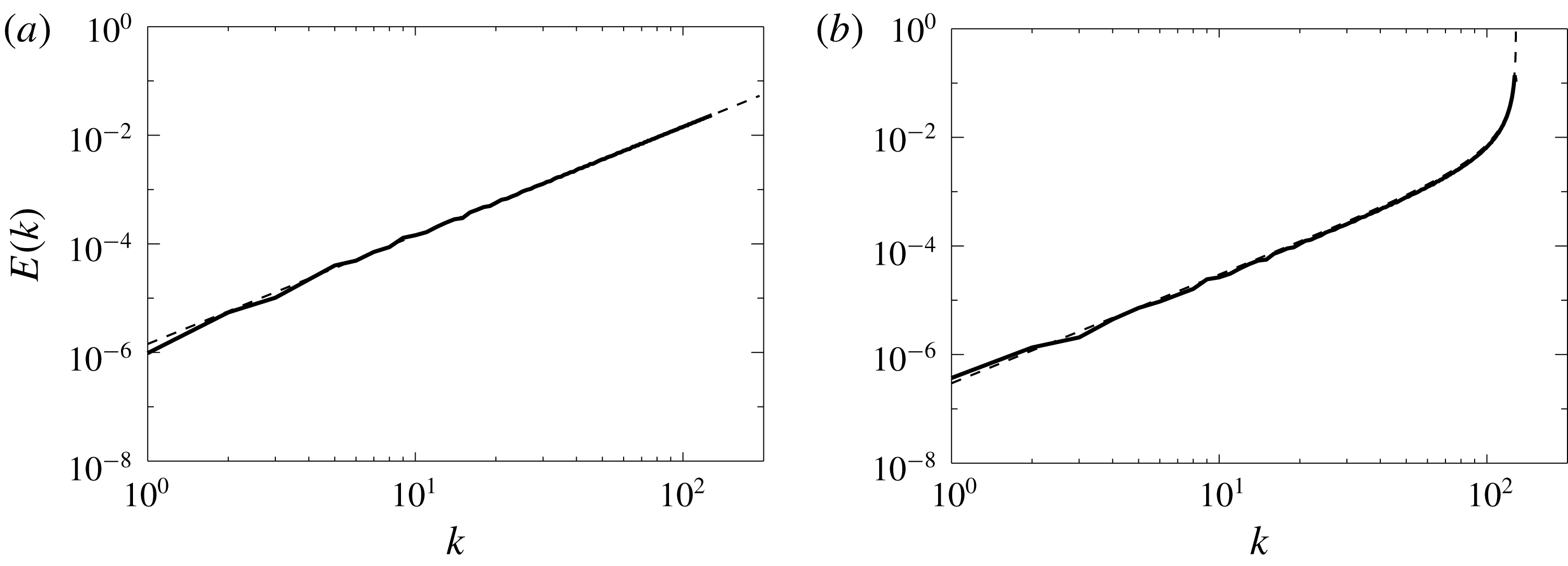
. A realization of the two spectra at late times obtained from two different numerical simulations of the truncated Euler equations with
 $k_{max}=128$
and zero helicity (a) and
 ${\mathcal{H}}/{\mathcal{E}}k_{max}=0.82$
(b) is shown in figure 1. The dashed lines show the theoretical predictions given in (1.4). Besides the energy spectum, the complex amplitudes of each Fourier mode were also shown to follow a Gaussian distribution in Cameron, Alexakis & Brachet (Reference Cameron, Alexakis and Brachet2017). Furthermore, the correlation time
 $\unicode[STIX]{x1D70F}_{\boldsymbol{k}}$
of the different Fourier modes can be calculated for the thermal equilibrium state and scales like
 $\unicode[STIX]{x1D70F}_{\boldsymbol{k}}\propto k^{-1}{\mathcal{E}}^{-1/2}$
for non-helical flows and
 $\unicode[STIX]{x1D70F}_{\boldsymbol{k}}\propto k^{-1/2}{\mathcal{H}}^{-1/2}$
for strongly helical flows (Cichowlas et al.
Reference Cichowlas, Bonaïti, Debbasch and Brachet2005; Cameron et al.
Reference Cameron, Alexakis and Brachet2017). These predictions have been verified with numerical simulations of the truncated Euler equations in numerous investigations (Cichowlas et al.
Reference Cichowlas, Bonaïti, Debbasch and Brachet2005; Krstulovic et al.
Reference Krstulovic, Mininni, Brachet and Pouquet2009; Cameron et al.
Reference Cameron, Alexakis and Brachet2017).
The energy spectra from two simulations of the truncated Euler equations with
 $k_{max}=128$
and zero helicity (a) and
 ${\mathcal{H}}/{\mathcal{E}}k_{max}=0.82$
(b). The dashed lines show the theoretical predictions given in (1.4).

Recent numerical simulations (Dallas, Fauve & Alexakis Reference Dallas, Fauve and Alexakis2015; Cameron et al.
Reference Cameron, Alexakis and Brachet2017) have revealed that the properties of the large scales in a forced turbulent flow are close to those predicted by the equilibrium statistical mechanics in Kraichnan (Reference Kraichnan1973). At steady state the energy spectra at large scales were shown to be close to a
 $k^{2}$
power law with Gaussian distribution of the complex amplitudes of the Fourier modes and the correlation times were also compatible with the
 $\unicode[STIX]{x1D70F}_{\boldsymbol{k}}\propto k^{-1}{\mathcal{E}}^{-1/2}$
prediction, at least for some range of scales. The agreement with the spectral and temporal predictions would indicate that the large scales in a turbulent flow are in equilibrium and can be described by such dynamics. However, some notable deviations both in the spectra and in the correlation time scales were also observed in Dallas et al. (Reference Dallas, Fauve and Alexakis2015), Cameron et al. (Reference Cameron, Alexakis and Brachet2017) and some care needs to be taken. This is what we will try to investigate in this work.
Strictly speaking absolute equilibrium statistical mechanics can be applied to isolated systems such that no energy injection or dissipation takes place. The large scales in the dissipative Navier–Stokes equations are different in many respects from the absolute equilibrium of the truncated Euler equations. First of all, in the truncated Euler equations the energy and helicity are conserved and determined solely by the initial conditions. For the large scales of the Navier–Stokes equations however, there is a constant exchange of energy with the forcing and turbulent scales by the nonlinearity that couples all modes. The large scales reach an equilibrium state such that only on average there is zero energy exchange with the forced and the turbulent scales. The energy contained in these scales is thus not determined by initial conditions but by the equilibration processes with the forced and turbulent scales. In other words, the large scales in a turbulent flow resemble a reservoir that is in a (non-local) contact with a second out-of-equilibrium reservoir consisting of the smaller (forced, turbulent and dissipative) scales.
This point of view leads to two possibilities. If the energy exchange fluctuations between the large and the small scales are relatively weak compared to the large-scale self-interactions then one expects that the large-scale spectrum will be indeed close to a thermal equilibrium state and will be universal. The role of the long-range interactions (between the large and the small scales) will only be to set the global energy (temperature) and helicity of the equilibrium state without altering the functional form of the spectrum that is determined by the local large-scale interactions. If on the other hand the long-range interactions are dominant, so that the large-scale self-interactions cannot respond fast enough to bring the system in equilibrium then the large scales can deviate from the equilibrium state and their statistical properties will be determined by the forcing and turbulent scales. Furthermore, if it is the interactions with the turbulent scales that determine the large-scale spectrum we expect again the large-scale spectrum to be universal. If however it is the interactions with the forcing scales that dominate, the large-scale spectrum will not be universal and will depend on the details of the forcing.
A related problem to the one we are addressing in this work is that of the behaviour of large scales in decaying three-dimensional turbulence. The large scales in decaying turbulence have been extensively investigated both theoretically and experimentally (Batchelor & Proudman Reference Batchelor and Proudman1956; Saffman Reference Saffman1967; Lesieur & Schertzer Reference Lesieur and Schertzer1978; George Reference George1992; Speziale & Bernard Reference Speziale and Bernard1992; Chasnov Reference Chasnov1994; Ristorcelli Reference Ristorcelli2003; Ishida, Davidson & Kaneda Reference Ishida, Davidson and Kaneda2006; Krogstad & Davidson Reference Krogstad and Davidson2010; Meldi & Sagaut Reference Meldi and Sagaut2012; Yoshimatsu & Kaneda Reference Yoshimatsu and Kaneda2018, Reference Yoshimatsu and Kaneda2019). The small wavenumber power-law behaviour can be shown to control the decay law of energy and two different possibilities have been noted in the literature. In one case is the so-called Saffman turbulence (due to Saffman’s seminal work (Saffman Reference Saffman1967)) where the power-law behaviour
 $E(k)\propto ({\mathcal{L}}/4\unicode[STIX]{x03C0}^{2})k^{2}+\cdots \,$
is expected and energy decays as
 $t^{-6/5}$
. The prefactor
 ${\mathcal{L}}=\int \langle \boldsymbol{u}(\boldsymbol{x})\boldsymbol{\cdot }\boldsymbol{u}(\boldsymbol{x}+\boldsymbol{r})\rangle \,\text{d}\boldsymbol{r}^{3}$
is known as the Saffman integral (Saffman Reference Saffman1967). If the initial conditions are such that the Saffman integral is zero, then a different type of decaying turbulence is met, the so-called Batchelor’s turbulence (due to Batchelor’s seminal earlier work (Batchelor & Proudman Reference Batchelor and Proudman1956)) where the energy spectrum scales like
 $E(k)\propto ({\mathcal{I}}/4\unicode[STIX]{x03C0}^{2})k^{4}+\cdots \,$
and the energy decays as
 $t^{-10/7}$
. Here,
 ${\mathcal{I}}=\int r^{2}\langle \boldsymbol{u}(\boldsymbol{x})\boldsymbol{\cdot }\boldsymbol{u}(\boldsymbol{x}+\boldsymbol{r})\rangle \,\text{d}\boldsymbol{r}^{3}$
is the Loitsyansky integral (Loitsianskii Reference Loitsianskii1939). Turbulence decay thus shows a sensitivity to the initial conditions, that sometimes also differs from Saffman’s and Batchelor’s ideal cases (Valente & Vassilicos Reference Valente and Vassilicos2012). Despite the fact that Saffman turbulence predicts the same exponent as the thermal equilibrium, decaying turbulence is considerably different from the forced case. First, in decaying turbulence the large scales are ever evolving and depend on initial conditions while in the forced case a statistical average in the long time limit is assumed where information about initial conditions is forgotten. Second, for the steady state problem the large scales also interact with (and are modified by) the forced scales that are absent in decaying turbulence. Thus, it is not possible to easily extrapolate from one case to the other.
In this work we try to answer the questions regarding the steady state problem with a set of numerical simulations. Our findings show that, at least for the examined values of the scale separations, both situations are feasible. The remaining presentation of this work is as follows. In § 2 we describe the exact set-up we are going to investigate and present the numerical simulations used. In § 3 we present the resulting large-scale energy spectra and large-scale structures, while in § 4 we present an analysis of the results by looking at the number of interacting triads, the amplitude of the nonlinearity spectrum, the flux due to interactions of different scales and different helicity and the energy transfer among the different scales. We draw our conclusions in the last section.
2 Set-up and numerical simulations
To investigate the dynamics of the large scales we performed a number of numerical simulations. The simulations follow the flow of an incompressible and unit density fluid in a triple periodic cube of size
 $2\unicode[STIX]{x03C0}$
. The flow satisfies the hyper-viscous Navier–Stokes equation,
 $$\begin{eqnarray}\displaystyle \unicode[STIX]{x2202}_{t}\boldsymbol{u}+\boldsymbol{u}\boldsymbol{\cdot }\unicode[STIX]{x1D735}\boldsymbol{u}=-\unicode[STIX]{x1D735}P-\unicode[STIX]{x1D708}_{4}\unicode[STIX]{x1D6E5}^{4}\boldsymbol{u}+\boldsymbol{f}, & & \displaystyle\end{eqnarray}$$
where
 $\boldsymbol{u}$
is the incompressible (
 $\unicode[STIX]{x1D735}\boldsymbol{\cdot }\boldsymbol{u}=0$
) velocity field,
 $P$
is the pressure,
 $\unicode[STIX]{x1D708}_{4}$
is the hyper-viscosity and
 $\boldsymbol{f}$
is the an externally imposed forcing. Since we are mostly interested in the behaviour of the large scales we have chosen a forcing that is concentrated around large Fourier wavenumbers with
 $|\boldsymbol{k}|\sim k_{f}=40$
. The use of hyper-viscosity was found to be necessary to avoid any molecular viscosity effects at the large scales. Carrying out the present simulations with regular viscosity
 $\unicode[STIX]{x1D708}$
at high enough Reynolds number
 $Re=u_{rms}/(\unicode[STIX]{x1D708}k_{f})$
(where
 $u_{rms}$
stands for the root mean square value of
 $u$
) so that the flow is turbulent while maintaining a large scale separation between the forcing scale and the domain size is not feasible with the available computational resources. As a result we cannot define a meaningful Reynolds number for our flow (a hyper-viscous Reynolds number
 $Re=u_{rms}/(\unicode[STIX]{x1D708}_{4}k_{f}^{7})\sim 10^{19}$
conveys very little information). We have verified however that for our choice of hyper-viscosity there is minimal dissipation at forcing scales and thus dissipation is achieved by the transfer of energy to the small scales (see also the fluxes in figure 11). We stress however that future simulations of higher scale separation would be required to verify the independence of
 $Re$
. The simulations were performed using the pseudospectral Ghost-code (Mininni et al.
Reference Mininni, Rosenberg, Reddy and Pouquet2011) with a second-order Runge–Kutta method for the time advancement and
 $2/3$
rule for dealiasing. For all runs we used a computational grid of size
 $N=1024$
in each of the three directions, and we tuned the value of the hyper-viscous coefficient so that the flow is well resolved.
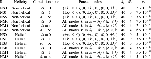
To test the effect of forcing on the large-scale modes
 $12$
different forcing functions were used that varied in helicity, their correlation time and the number of forced modes. In particular, regarding the helicity two options were considered. Either the forcing was chosen such that every realization was fully helical
 $\unicode[STIX]{x1D735}\times \boldsymbol{f}=k_{f}\boldsymbol{f}$
or it had exactly zero helicity
 $\langle \boldsymbol{f}\boldsymbol{\cdot }\unicode[STIX]{x1D735}\times \boldsymbol{f}\rangle =0$
(where brackets stand for spatial average). We refer to these two types of forcing as helical and the non-helical forcing.
The second parameter we varied was the number of Fourier modes that were forced. Two choices were examined. In the first choice the forced modes
 $\boldsymbol{k}=(k_{x},k_{y},k_{z})$
were the six modes on the faces of the
 $k_{f}$
-cube
 $(\pm k_{f},0,0),(0,\pm k_{f},0),(0,0,\pm k_{f})$
with
 $k_{f}=40$
. This case corresponds to an ABC forcing if helical, or to its non-helical version sometimes referred as the CBA forcing (Cameron et al.
Reference Cameron, Alexakis and Brachet2017). We refer to the flows with this forcing as the six-mode forced flows. The other choice was to force all Fourier modes inside a spherical shell of external radius
 $k_{f}=40$
and internal radius
 $k_{f}-\unicode[STIX]{x1D6FF}k_{f}=36$
. This forcing corresponds to a random (almost) isotropic forcing and we will refer to this forcing as multi-mode forcing.
Table of runs. For all runs the resolution in each direction was
 $N=1024$
. The
 $\unicode[STIX]{x1D6FF}t=\infty$
implies that the forcing was constant in time,
 $\unicode[STIX]{x1D6FF}t=1$
implies that the forcing was changed randomly approximately every turnover time and
 $\unicode[STIX]{x1D6FF}t=0$
implies that the forcing changed randomly every time step.

Finally, the last parameter we varied was the correlation time of the forcing. The phases of the forcing modes
 $\tilde{\boldsymbol{f}}_{\boldsymbol{k}}$
were changed randomly every time interval
 $\unicode[STIX]{x1D6FF}t$
. Three choices for the correlation time
 $\unicode[STIX]{x1D6FF}t$
were made: (i) it was either infinite,
 $\unicode[STIX]{x1D6FF}t=\infty$
, (so that
 $\boldsymbol{f}$
was independent of time), (ii) it was finite and close to the turnover time
 $\unicode[STIX]{x1D6FF}t\simeq 1/(k_{f}{\mathcal{E}}^{1/2})$
or (iii) the phases were changed every numerical time step
 $\unicode[STIX]{x1D6FF}t=dt$
with the amplitude of the forcing scaling like
 $1/\sqrt{dt}$
. In the last case the forcing is approximately delta correlated in time, fixing in this way the energy injection rate
 $\unicode[STIX]{x1D716}$
. The parameters of all the runs are given in table 1. Each simulation was run for a sufficiently long time so that the energy spectrum reached a statistically steady state such that the energy, even at the smallest wavenumbers
 $k=1,2$
, fluctuated around a mean value. We note that the distribution of the energy at large scales took a considerably longer time to saturate (compared to the time in which the total energy saturates). Effectively each simulation was performed for a few hundred turnover times
 $\unicode[STIX]{x1D70F}_{{\mathcal{E}}}=k_{f}^{-1}{\mathcal{E}}^{-1/2}$
.
3 Large-scale spectra and structures
3.1 Spectra
We begin by examining the energy spectra of the different flows. The energy spectra are output frequently throughout the numerical simulation and are time averaged in the steady state regime. This averaging is particularly important for the time-dependent six-mode forced runs that displayed large fluctuations in the large-scale energy spectra, and a spectrum calculated from a single time realization of the flow field can considerably deviate from the time-averaged value.
The spectra are shown in figure 2(a–d) for the 12 different runs examined in this work. They are compensated by
 $k^{-2}$
so that a thermal spectrum
 $k^{2}$
will appear as flat. Non-compensated spectra are plotted in the insets. Non-helical runs are displayed on (a,b) while helical runs are displayed in (c,d). Runs with six-mode forcing are displayed in the panels on the left while runs with multi-mode forcing are displayed in the panels on the right. The three different lines in each panel correspond to the three different correlation times used. The darkest line corresponds to the delta correlated in time forcing, while the lightest grey line corresponds to the time-independent forcing.
Energy spectra
 $E(k)$
compensated by
 $k^{-2}$
for the 12 different runs given in table 1. (a–d) Show the spectra for the non-helical/helical flows and (a,c), (b,d) show the spectra for the six-mode/multi-mode forced flows. The insets show the same spectra uncompensated.

The differences of the energy spectra at the large scales among the different runs are striking. Flows with six-mode forcing are very close to the thermal equilibrium spectrum
 $E(k)\propto k^{2}$
. This is most clear for the helical flows (figure 2
c) for which all three cases show a clear
 $k^{2}$
scaling. We need to note here that although the forcing was fully helical in these flows the amount of helicity that was transferred to the large scales remained minimal. For this reason these flows also equilibrate to a thermal state with
 $\unicode[STIX]{x1D6FD}\simeq 0$
(see (1.4)).
Non-helical six-mode forcing flows also saturate close to the thermal equilibrium spectrum (figure 2
a). The spectrum of the flow with the delta correlated forcing is particularly close to a
 $k^{2}$
spectrum while the flows with finite correlation time and infinite correlation time showed a slightly smaller exponent than 2. This was also observed for the infinite correlation time non-helical forcing in Cameron et al. (Reference Cameron, Alexakis and Brachet2017). The series of peaks in the spectrum that appear for these flows at wavenumbers larger than the forcing are due to self-interactions between forcing modes that excite first velocity modes with wavevectors of module
 $\sqrt{2}k_{f}$
.
The flows with a multi-mode forcing deviate from the thermal prediction (figure 2
b,d). This effect is relatively weak for the flows with short-time correlated forcing but very strong for the time independent forcing where a strong peak (for the compensated spectra) appears at the largest scales of the spectrum at
 $k=1$
. This is true both for the helical and the non-helical forcing however the deviation is stronger for the non-helical forcing. The non-compensated spectra appear almost flat in this case. The helical runs appear to satisfy the
 $k^{2}$
law for a short range close to
 $k_{f}$
but have a strong deviation at the largest scales
 $k<10$
.
Helicity spectra
 $H(k)$
compensated by
 $k^{-4}$
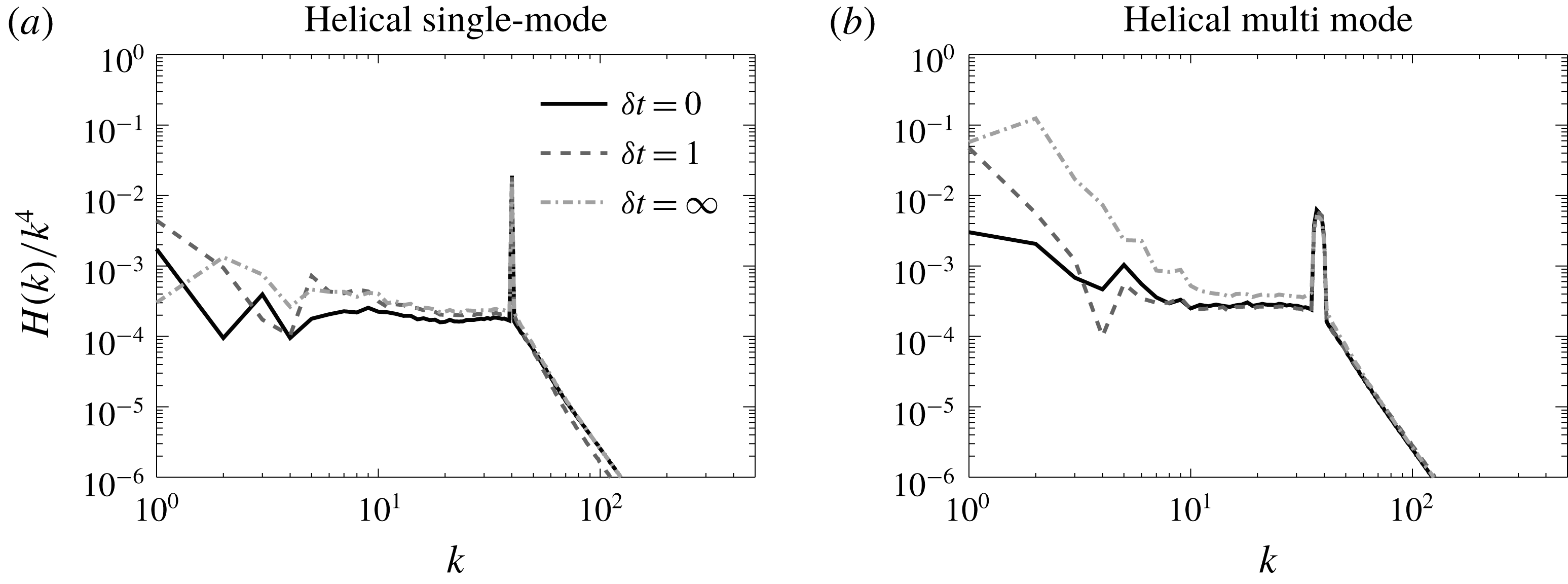
for the 6 different helical runs given in table 1. (a) is for the six-mode forced flows and (b) is for the multi-mode forced flows.

For completeness we also show in figure 3 the helicity spectra
 $H(k)$
compensated by
 $k^{-4}$
. Similar to the energy spectra the helical six-mode forced runs have a helicity spectrum close to the absolute equilibrium solution
 $k^{4}$
for all correlation times. However, because
 $H(k)$
is a sign-indefinite quantity the fluctuations are larger. For the multi-scale forcing we see again significant deviations from the
 $k^{4}$
power law. This effect is again strongest for the infinite correlated forcing for which a large peak at
 $k=1$
and
 $k=2$
appears for the compensated spectra.
3.2 Spatial structures
In figure 4 we show, using the graphics package vapor (Clyne et al.
Reference Clyne, Mininni, Norton and Rast2007), a three-dimensional iso-surface visualization of the energy for the truncated Euler system (a) and for two forced runs: one that displayed the
 $k^{2}$
spectrum at large scales HS0 (b) and one that displayed strong deviations from the
 $k^{2}$
spectrum NM8 (c). (a,c) Display a flow that is completely featureless. All energy is concentrated uniformly at the small (forcing) scales resembling white noise. The same is almost true for the flow displayed in the panel on the right, however some clustering of the large-scale structures can be seen. The visualization of the structures in physical space thus conveys little information.
A three-dimensional iso-surface visualization of the energy density for three different flows: (a) the truncated Euler system on the left, (b) the helical six-mode run with
 $\unicode[STIX]{x1D6FF}t=0$
HS0 that displayed a
 $k^{2}$
spectrum at the large scales, (c) the non-helical multi-mode run with
 $\unicode[STIX]{x1D6FF}t=\infty$
NM8 that displayed a
 $k^{0}$
spectrum at the large scales.

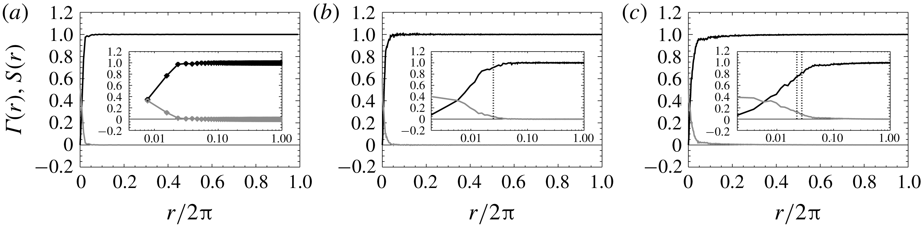
The correlation function
 $\unicode[STIX]{x1D6E4}(r)$
(grey line) and the structure function
 $S(r)$
(black line) for (a) the truncated Euler system in the left, (b) the helical six-mode run with
 $\unicode[STIX]{x1D6FF}t=0$
HS0 that displayed a
 $k^{2}$
spectrum at the large scales, (c) the non-helical multi-mode run with
 $\unicode[STIX]{x1D6FF}t=\infty$
NM8 that displayed a
 $k^{0}$
spectrum at the large scales. The insets show the same plots in linear–logarithmic scale. The vertical doted lines indicate the spatial period of the forcing.

For a more quantitative look at the spatial structures we define the the correlation function
 $\unicode[STIX]{x1D6E4}(r)$
and the second-order structure function
 $S(r)$
as
 $$\begin{eqnarray}\unicode[STIX]{x1D6E4}(r)=\langle (\boldsymbol{u}(\boldsymbol{x})\boldsymbol{\cdot }\hat{\boldsymbol{r}})(\boldsymbol{u}(\boldsymbol{x}+\boldsymbol{r})\boldsymbol{\cdot }\hat{\boldsymbol{r}})\rangle ,\quad S(r)=\langle [(\boldsymbol{u}(\boldsymbol{x})-\boldsymbol{u}(\boldsymbol{x}+\boldsymbol{r}))\boldsymbol{\cdot }\hat{\boldsymbol{r}}]^{2}\rangle ,\end{eqnarray}$$
where
 $\hat{\boldsymbol{r}}$
is the unit vector along
 $\boldsymbol{r}$
and the angular brackets stand for the spatial average over the variable
 $\boldsymbol{x}$
. The two functions are connected by
 $S(r)=(4/3){\mathcal{E}}-2\unicode[STIX]{x1D6E4}(r)$
for isotropic fields. The correlation function is also connected to the energy spectrum, being its Fourier transform based on the Wiener–Khinchin theorem (Chatfield Reference Chatfield2016). The two functions are shown in figure 5 in linear scale, for the truncated Euler flow on the right, the Helical six-mode forced flow HS0 in the middle and for the non-helical multi-mode forced run to the right. The inset displays the same graphs in linear–logarithmic scale that focuses on the small
 $r$
region.
For the truncated Euler flow the correlation function resembles a Dirac delta function: only the first two points are non-zero, while the remaining points attain very small (both positive and negative) values. Similarly, the structure function attains its asymptotic value within the first points. The amplitude of
 $\unicode[STIX]{x1D6E4}(r)$
for
 $r>0.02$
is decreasing as the size of the sample of points used is increased and is expected to become exactly zero when the sample size goes to infinity. This is what is expected from a thermalized state for which each degree of freedom acts as an independent Gaussian random variable. The reason for which not only the
 $r=0$
point is non-zero but the first two points as well is because of the de-aliasing that is performed in the numerical simulations. The de-aliasing removes
 $1/3$
of all Fourier modes and as a result there are more grid points than true degrees of freedom (counted by the active Fourier modes). Thus there is some correlation remaining between neighbouring points in physical space.
A similar behaviour is observed in the forced runs, only in this case the flows remain correlated up to the forcing scales, after which
 $\unicode[STIX]{x1D6E4}(r)$
decreases sharply reaching very small (both positive and negative) values. We note that this noisy behaviour at large
 $r$
with alternating signs does not allow us to use a log–log scale to determine if this sudden drop is exponential or power law. We only note that for the right panel this drop appears to be slightly slower than in the central panel as is also expected from the spectra.
4 Analysis
The presented spectra suggest that the large-scale spectrum of the steady state of forced turbulence does not have a universal character and can be affected by the details of the forcing that excites the flow. In what follows we try to analyse the origin of these deviations by looking at the number of interacting triads, the amplitude of the nonlinearities at the large scales and the energy transfer properties of the flow at large scales.
4.1 Interacting triads
Perhaps the strong deviations for the multi-mode forcing could have been anticipated. In the case that only six modes are forced, the forced modes do not directly interact with large-scale modes, while the multi-mode forcing allows forcing mode interactions that directly couple with the large scales.
In more detail, for the six-mode forcing the wavenumbers that are forced are given by
 $\boldsymbol{k}_{1},\boldsymbol{k}_{2}\in [(\pm k_{f},0,0),(0,\pm k_{f},0),(0,0,\pm k_{f})]$
. If we consider two velocity modes with wavenumbers
 $\boldsymbol{k}_{1},\boldsymbol{k}_{2}$
that belong to these forcing modes then they can interact with a third wavenumber
 $\boldsymbol{q}$
that forms the triad
 $\boldsymbol{q}+\boldsymbol{k}_{1}+\boldsymbol{k}_{2}=0$
. The allowed
 $\boldsymbol{q}$
values for which there is non-zero energy transfer are
 $\boldsymbol{q}\in [(\pm k_{f},\pm k_{f},0),(\pm k_{f},0,\pm k_{f}),(0,\pm k_{f},\pm k_{f})]$
. The
 $\boldsymbol{q}=\mathbf{0}$
as well as the
 $\boldsymbol{q}=[(\pm 2k_{f},0,0),(0,\pm 2k_{f},0),(0,0,\pm 2k_{f})]$
cases, although allowed by the triad condition
 $\boldsymbol{q}+\boldsymbol{k}_{1}+\boldsymbol{k}_{2}=0$
, lead to zero nonlinearity and do not transfer any energy. Thus the forced velocity modes only excite directly modes with
 $|q|=\sqrt{2}k_{f}$
and therefore smaller scales than the forcing scale. This does not mean that large scales cannot be excited. They can be excited by interactions of the form
 $\boldsymbol{k}+\boldsymbol{q}_{1}+\boldsymbol{q}_{2}=0$
where only
 $\boldsymbol{k}\in [(\pm k_{f},0,0),(0,\pm k_{f},0),(0,0,\pm k_{f})]$
or by the subsequent interactions between the large and turbulent scales. However since the forced velocity modes are in general stronger, at large scales, interactions which involve only one or no forced mode
 $\boldsymbol{k}$
tend to be weaker than those with two forced modes.
A multi-mode forcing, on the other hand, allows forcing mode interactions that directly affect the large scales. This occurs because, among the many modes that reside inside the spherical shell of external radius
 $k_{f}$
and width
 $\unicode[STIX]{x1D6FF}k_{f}$
(that we denote as
 $K_{F}$
), one can find many combinations of forced velocity modes
 $\boldsymbol{k}_{1},\boldsymbol{k}_{2}$
that can form a triad
 $\boldsymbol{q}+\boldsymbol{k}_{1}+\boldsymbol{k}_{2}=0$
provided that
 $|\boldsymbol{q}|\leqslant 2k_{f}$
. Thus energy can be transferred directly to large-scale modes
 $q<k_{f}$
. More precisely it is shown in appendix A that the number of triads
 $N_{Q}$
that are allowed between the modes inside a spherical shell
 $Q$
of radius
 $q$
and width
 $1$
with the forcing modes at
 $K_{F}$
are given by
 $$\begin{eqnarray}\displaystyle N_{Q}\simeq 16\unicode[STIX]{x03C0}^{2}k_{f}^{2}\unicode[STIX]{x1D6FF}k_{f}q^{2}\quad \text{for }q\ll \unicode[STIX]{x1D6FF}k_{f}\ll k_{f} & & \displaystyle\end{eqnarray}$$
and
 $$\begin{eqnarray}\displaystyle N_{Q}\simeq 8\unicode[STIX]{x03C0}^{2}k_{f}^{2}\unicode[STIX]{x1D6FF}k_{f}^{2}q\quad \text{for }\unicode[STIX]{x1D6FF}k_{f}\ll q\ll k_{f}. & & \displaystyle\end{eqnarray}$$
The multi-mode forcing thus leads to interactions with the forcing modes that have a power-law distribution with the modulus of the large-scale wavenumbers
 $q$
. The index of this power law depends on the relative magnitude of
 $q$
with
 $\unicode[STIX]{x1D6FF}k_{f}$
.
Therefore, the density of forced modes can alter significantly the number of allowed triads that couple forced modes with large-scale modes. The ‘sparse’ six-mode forcing leads to no direct interactions while the ‘dense’ multi-scale forcing leads to a power-law distribution of such triads. It is thus not surprising that the forced mode density can affect the large-scale spectrum.
4.2 Spectrum of the nonlinearity
Besides the density of these interactions their amplitude should also be examined to draw conclusions. Energy injected at the forcing scales is redistributed among all Fourier modes of the flow by the nonlinear term of the Navier–Stokes equation. To understand how the large scales come to thermal equilibrium and the origins of the deviations from it we analyse the nonlinear term of the Navier–Stokes equation by looking at its spectrum and its different components.
The nonlinearity of the Navier–Stokes equation
 ${\mathcal{N}}(\boldsymbol{x})$
is given by
 $$\begin{eqnarray}\displaystyle \boldsymbol{{\mathcal{N}}}(\boldsymbol{x})=\boldsymbol{u}\boldsymbol{\cdot }\unicode[STIX]{x1D735}\boldsymbol{u}+\unicode[STIX]{x1D735}P=\boldsymbol{u}\boldsymbol{\cdot }\unicode[STIX]{x1D735}\boldsymbol{u}-\unicode[STIX]{x1D735}\unicode[STIX]{x1D6E5}^{-1}\unicode[STIX]{x1D735}\boldsymbol{\cdot }(\boldsymbol{u}\boldsymbol{\cdot }\unicode[STIX]{x1D735}\boldsymbol{u}), & & \displaystyle\end{eqnarray}$$
where in the second equality we have written an explicit expression for the pressure
 $$\begin{eqnarray}\displaystyle P=-\unicode[STIX]{x1D6E5}^{-1}\unicode[STIX]{x1D735}\boldsymbol{\cdot }(\boldsymbol{u}\boldsymbol{\cdot }\unicode[STIX]{x1D735}\boldsymbol{u}), & & \displaystyle\end{eqnarray}$$
with
 $\unicode[STIX]{x1D6E5}^{-1}$
standing for the inverse Laplacian. The nonlinearity
 ${\mathcal{N}}(\boldsymbol{x})$
is a divergence-free vector field that depends on space. We can therefore define its Fourier transform
 $$\begin{eqnarray}\displaystyle \tilde{{\mathcal{N}}}(\boldsymbol{k})=\frac{1}{(2\unicode[STIX]{x03C0})^{3}}\int {\mathcal{N}}(\boldsymbol{x})\text{e}^{\text{i}\boldsymbol{k}\boldsymbol{x}}\,\text{d}x^{3}, & & \displaystyle\end{eqnarray}$$
and define its spectrum as
 $$\begin{eqnarray}\displaystyle E_{{\mathcal{N}}}(k)=\mathop{\sum }_{k\leqslant |\boldsymbol{k}|<k+1}|\tilde{{\mathcal{N}}}(\boldsymbol{k})|^{2}. & & \displaystyle\end{eqnarray}$$
The spectrum
 $E_{{\mathcal{N}}}(k)$
gives a measure of the amplitude of the nonlinear term at the given shell of wavenumber
 $k$
.
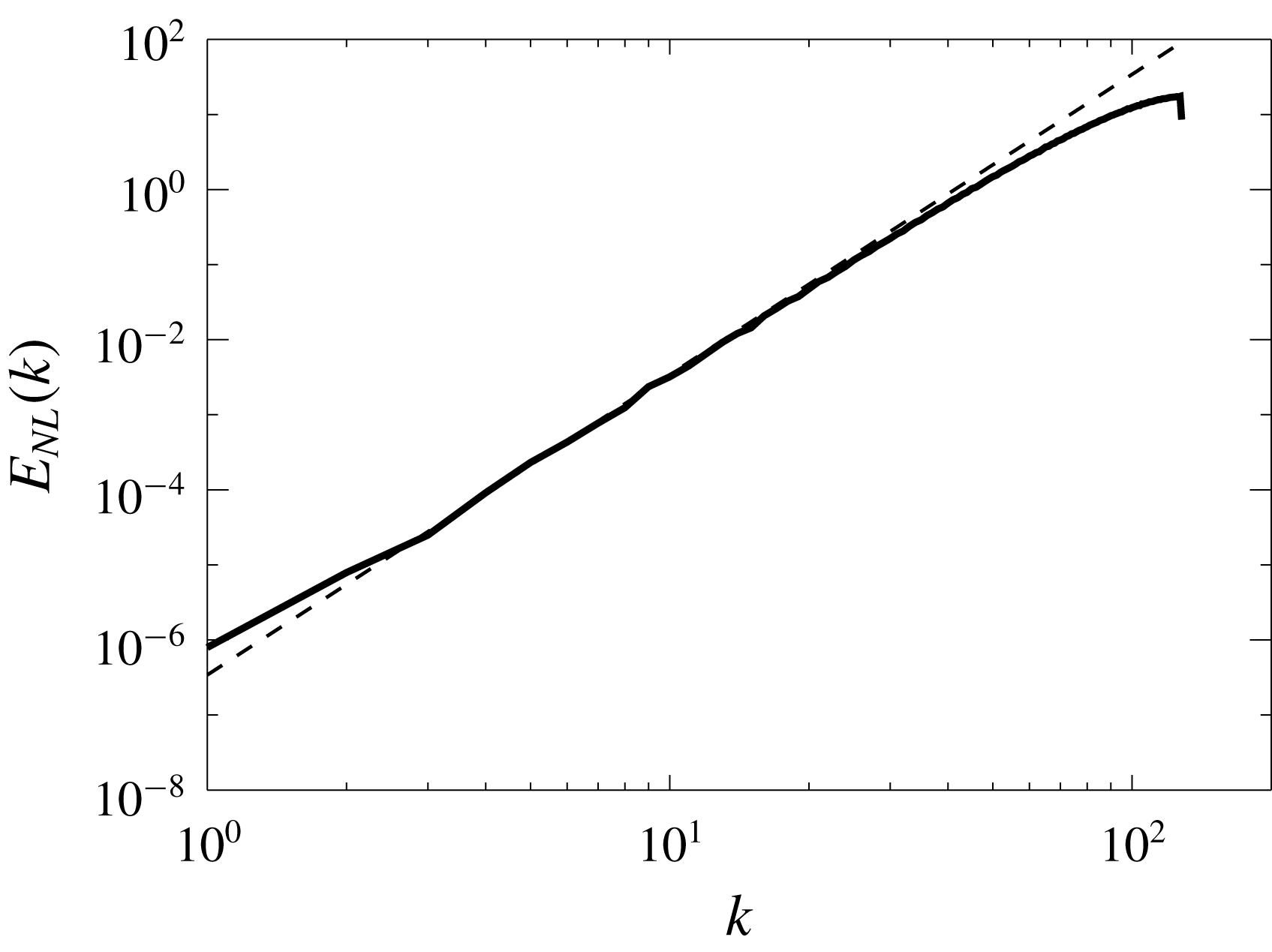
For the truncated Euler equations where the flow reaches a thermal equilibrium state the spectrum of the nonlinearity can be calculated exactly. This is done in appendix B and leads to the prediction
 $$\begin{eqnarray}\displaystyle E_{{\mathcal{N}}}(q)=\frac{14{\mathcal{E}}^{2}}{5k_{max}^{3}}q^{4}. & & \displaystyle\end{eqnarray}$$
A comparison of this result with
 $E_{{\mathcal{N}}}(q)$
obtained from numerical simulations of flows obeying the truncated Euler equations (1.1) is shown in figure 6. Similar estimates (although no longer rigorous) can be made for the forced flows if some extra assumptions are made. These calculations are presented in appendix C and lead to the predictions
 $$\begin{eqnarray}\displaystyle E_{{\mathcal{N}}}(q)\propto q^{4}, & & \displaystyle\end{eqnarray}$$
if the energy spectrum
 $E(k)$
varies smoothly over distances of order
 $q$
or
 $$\begin{eqnarray}\displaystyle E_{{\mathcal{N}}}(q)\propto q^{3}, & & \displaystyle\end{eqnarray}$$
if the interactions are dominated by interactions with modes in a thin spherical shell (as for example with the forced modes in the multi-mode forcing flows) with
 $\unicode[STIX]{x1D6FF}k_{f}\ll q\ll k_{f}$
.
The spectrum
 $E_{{\mathcal{N}}}(k)$
of the nonlinearity obtained from the truncated Euler simulations (solid line) compared with the theoretical prediction (4.7).

The spectrum
 $E_{{\mathcal{N}}}(k)$
of the nonlinearity, normalized by
 $k^{4}$
. (a–d) are for the non-helical/helical flows and (a,c), (b,d) show the spectra for the six-mode/multi-mode forced flows. The dashed lines indicate the power laws
 $k^{0},k^{-1}$
that correspond to
 $k^{4}$
and
 $k^{3}$
for the uncompensated spectra (indicated also in the inset).

The compensated spectra
 $E_{{\mathcal{N}}}(k)/k^{4}$
for the twelve runs examined are shown in figure 7. The six-mode forcing simulations (for which there are no direct interactions with the forced modes at large scales) result in a spectrum for the nonlinearity close to
 $E_{{\mathcal{N}}}(k)\propto k^{4}$
. These are the flows that were also shown to develop energy spectra close to the ones predicted by the thermal equilibrium. The scaling appears to be valid both for the helical and the non-helical runs although is perhaps clearer for the non-helical runs. The multi-mode forced flows (that allow direct interactions with the forced modes) resulted in spectra that are closer to
 $E_{N}(k)\propto k^{3}$
. This suggests that the forcing modes that are restricted in a this spherical shell are important for the evolution of the large-scale modes as they can deform the spectrum of the nonlinearity at the large scales.
Another quantity that is of interest is the spectrum of the pressure,
 $$\begin{eqnarray}\displaystyle E_{P}(k)=\mathop{\sum }_{k\leqslant |\boldsymbol{k}|<k+1}|\tilde{P}(\boldsymbol{k})|^{2}, & & \displaystyle\end{eqnarray}$$
where
 $\tilde{P}$
stands for the Fourier transform of the pressure field obtained by (4.4). The great advantage of the pressure spectrum as opposed to the spectrum of the nonlinearity is that pressure can be measured in the laboratory (Willmarth & Wooldridge Reference Willmarth and Wooldridge1962; Corcos Reference Corcos1964; Abry et al.
Reference Abry, Fauve, Flandrin and Laroche1994; Tsuji et al.
Reference Tsuji, Fransson, Alfredsson and Johansson2007; van Oudheusden Reference van Oudheusden2013) and thus this prediction can also be tested in experiments.
The same arguments that were made in appendix C for the nonlinearity can be made for the gradient of the pressure
 $\unicode[STIX]{x1D735}P$
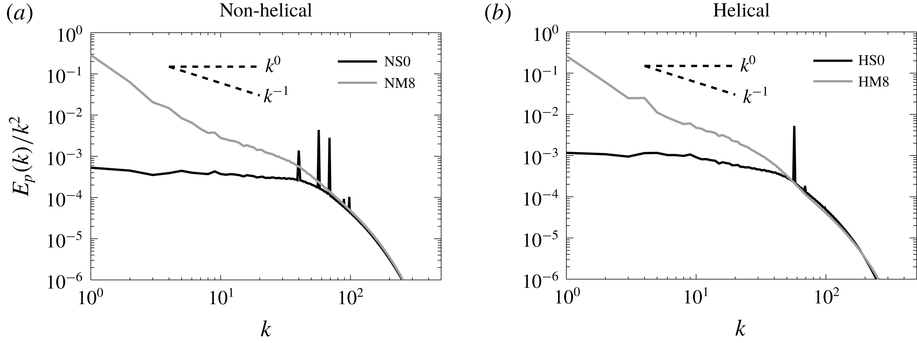
. We can therefore also make a prediction for the pressure spectrum. The pressure spectrum then should scale like
 $E_{P}(k)\propto E_{N}(k)k^{-2}$
and therefore it is expected to scale like
 $k^{2}$
for the six-mode forced flows and like
 $k^{1}$
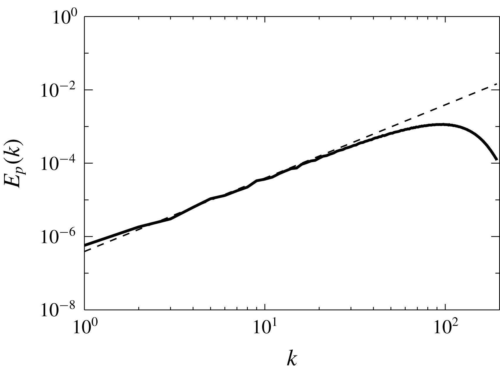
for the multi-mode forced flows. For the truncated Euler flows at thermal equilibrium, the pressure can be evaluated exactly (see appendix B) and it is given by
 $$\begin{eqnarray}\displaystyle E_{P}(q)=\frac{16{\mathcal{E}}^{2}}{5k_{max}^{3}}k^{2}. & & \displaystyle\end{eqnarray}$$
A comparison of this result with
 $E_{P}(q)$
obtained from numerical simulations is shown in figure 8 showing excellent agreement. For the forced runs, the pressure spectrum is shown in figure 9 the for cases NS0, HS0, NM8, HM8 normalized by
 $k^{2}$
. The spectra are compatible with the aforementioned predictions with the six-mode forced runs being close to a
 $k^{2}$
spectrum and the multi-mode forced runs closer to a
 $k^{1}$
spectrum.
The pressure spectrum
 $E_{P}(k)$
obtained from the truncated Euler simulations (solid line) compared with the theoretical prediction (4.11).

Spectrum of the pressure field
 $E_{P}(k)$
for the non-helical runs NS0, NM8 (a) and for the helical runs HS0, HN8 (b). The dark lines correspond to the six-mode forced runs with
 $\unicode[STIX]{x1D6FF}t=0$
(NS0, HS0) and the light grey lines correspond to the multi-mode forced runs with
 $\unicode[STIX]{x1D6FF}t=\infty$
.

4.3 The effect of different scales
To further illuminate the role of interactions among different scales and understand which ones lead the large scales to reach an equilibrium we decompose the velocity field in to three components
 $$\begin{eqnarray}\displaystyle \boldsymbol{u}=\boldsymbol{u}_{L}+\boldsymbol{u}_{F}+\boldsymbol{u}_{T} & & \displaystyle\end{eqnarray}$$
the large-scale flow
 $\boldsymbol{u}_{L}$
, the forcing-scale flow
 $\boldsymbol{u}_{F}$
and the turbulent-scale flow
 $\boldsymbol{u}_{T}$
. The three flows are defined as
 $$\begin{eqnarray}\displaystyle \boldsymbol{u}_{L}=\mathop{\sum }_{|\boldsymbol{k}|<k_{f}-\unicode[STIX]{x1D6FF}k_{f}}\tilde{\boldsymbol{u}}_{\boldsymbol{k}}\text{e}^{\text{i}\boldsymbol{k}\boldsymbol{x}},\quad \boldsymbol{u}_{F}=\mathop{\sum }_{k_{f}-\unicode[STIX]{x1D6FF}k_{f}\leqslant |\boldsymbol{k}|\leqslant k_{f}}\tilde{\boldsymbol{u}}_{\boldsymbol{k}}\text{e}^{\text{i}\boldsymbol{k}\boldsymbol{x}},\quad \boldsymbol{u}_{T}=\mathop{\sum }_{k_{f}<|\boldsymbol{k}|}\tilde{\boldsymbol{u}}_{\boldsymbol{k}}\text{e}^{\text{i}\boldsymbol{k}\boldsymbol{x}}. & & \displaystyle\end{eqnarray}$$
Given this decomposition the nonlinearity can be written as the sum of 9 terms explicitly given by
 $$\begin{eqnarray}\displaystyle \boldsymbol{{\mathcal{N}}}(\boldsymbol{x})=\mathop{\sum }_{I,J}\mathbb{P}[\boldsymbol{u}_{I}\boldsymbol{\cdot }\unicode[STIX]{x1D735}\boldsymbol{u}_{J}], & & \displaystyle\end{eqnarray}$$
where
 $\mathbb{P}$
stands for the projector operator to incompressible flows,
 $I,J$
stand for the indices
 $L,F,T$
and the sum is over all possible permutations. If we symmetrize over the change of two indices we obtain the following six nonlinear terms:
 $$\begin{eqnarray}\displaystyle \left.\begin{array}{@{}c@{}}{\mathcal{N}}_{LL}=\mathbb{P}[\boldsymbol{u}_{L}\boldsymbol{\cdot }\unicode[STIX]{x1D735}\boldsymbol{u}_{L}],\quad {\mathcal{N}}_{FF}=\mathbb{P}[\boldsymbol{u}_{F}\boldsymbol{\cdot }\unicode[STIX]{x1D735}\boldsymbol{u}_{F}],\quad {\mathcal{N}}_{TT}=\mathbb{P}[\boldsymbol{u}_{T}\boldsymbol{\cdot }\unicode[STIX]{x1D735}\boldsymbol{u}_{T}]\\ {\mathcal{N}}_{LF}=\mathbb{P}[\boldsymbol{u}_{L}\boldsymbol{\cdot }\unicode[STIX]{x1D735}\boldsymbol{u}_{F}+\boldsymbol{u}_{F}\boldsymbol{\cdot }\unicode[STIX]{x1D735}\boldsymbol{u}_{L}],\quad {\mathcal{N}}_{LT}=\mathbb{P}[\boldsymbol{u}_{L}\boldsymbol{\cdot }\unicode[STIX]{x1D735}\boldsymbol{u}_{T}+\boldsymbol{u}_{T}\boldsymbol{\cdot }\unicode[STIX]{x1D735}\boldsymbol{u}_{L}],\\ \text{and}\quad {\mathcal{N}}_{TF}=\mathbb{P}[\boldsymbol{u}_{T}\boldsymbol{\cdot }\unicode[STIX]{x1D735}\boldsymbol{u}_{F}+\boldsymbol{u}_{F}\boldsymbol{\cdot }\unicode[STIX]{x1D735}\boldsymbol{u}_{T}].\end{array}\right\} & & \displaystyle\end{eqnarray}$$
The first three represent the nonlinearity due to self-interactions of the large scales, forcing scales and turbulent scales while the remaining three represent cross-interactions. The sum of all six terms recovers the nonlinearity
 ${\mathcal{N}}(\boldsymbol{x})$
.
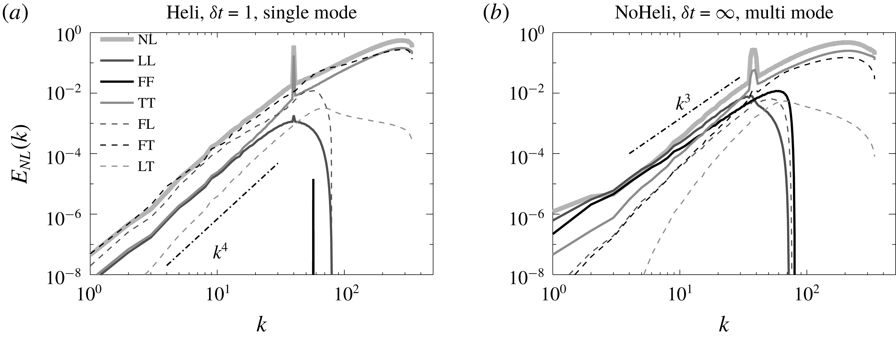
The spectra for the six different nonlinear terms given in (4.15) for the flows HS1 (helical, six-mode forced,
 $\unicode[STIX]{x1D6FF}t=1$
(a)) and NM8 (non-helical, multi-mode forced,
 $\unicode[STIX]{x1D6FF}t=\infty$
, (b)). The index
 $NL$
indicates the spectrum of the full nonlinearity, while the remaining indices indicate the spectra of the nonlinearities as given in equation (4.15).

As before we can calculate the spectra for each of the six nonlinear terms. We have done this for the six-mode forced run HS1 (helical, six mode,
 $\unicode[STIX]{x1D6FF}t=1$
) that is a characteristic example that displays a thermal equilibrium spectrum and NM8 (non-helical, multi-mode,
 $\unicode[STIX]{x1D6FF}t=\infty$
) that is a characteristic example of a flow that deviates from this spectrum. The spectra of the six nonlinear terms for these flows are shown in figure 10. In both cases the small scales are dominated by TT interactions as expected. At large scales however differences can be seen. For the flow HS1 the FF interactions are absent. They only appear as a single peak at
 $k=\sqrt{2}k_{f}$
. The most dominant interactions at the large scales appear to be the FL and FT interactions followed by LL and TT interactions. All terms appear to display a
 $k^{4}$
power law at large scales. In this case therefore it appears that all scales play a role in the formation of the large-scale spectrum.
On the other hand for the flow NM8 the most dominant interactions are with the forcing modes FF and the self-interactions of the large-scale LL. The FF and LL interactions appear to follow a clear
 $k^{3}$
power law at large scales while the other terms appear to have a slightly steeper behaviour. This implies that in this case the large-scale spectrum is determined by a balance between the forcing scales and the large-scale self-interactions. Furthermore, since these interactions follow a less steep scaling from the rest they become more dominant as smaller wavenumbers are reached.
This analysis therefore demonstrates that for the multi-mode forcing it is the interactions with forcing modes that dominate and the deviations from the thermal equilibrium spectrum can be attributed to them. The self-interactions of the large scales, which are of similar amplitude, try to restore the equilibrium as we will demonstrate in the next subsections.
4.4 Energy fluxes
The spectra examined in the previous section give some information regarding the amplitude of different interactions at the large scales. However, they do not provide direct information on how much energy is added or extracted from these scales due to those particular interactions. The rate of exchange of energy can be extracted by looking at the flux of energy.
The flux of energy through a spherical shell in Fourier space of radius
 $k$
is defined as
 $$\begin{eqnarray}\displaystyle \unicode[STIX]{x1D6F1}(k)=\langle \boldsymbol{u}^{{<}k}\boldsymbol{\cdot }\boldsymbol{{\mathcal{N}}}\rangle , & & \displaystyle\end{eqnarray}$$
where
 $\boldsymbol{u}^{{<}k}$
is the velocity field filtered so that only Fourier modes of wavenumbers smaller than
 $k$
are retained. For three-dimensional high
 $Re$
turbulent flows the time-averaged flux
 $\unicode[STIX]{x1D6F1}(k)$
is zero for wavenumbers smaller than the forcing, is equal to the energy injection rate at the inertial scales and drops back to zero at the dissipative scales. The fact that
 $\unicode[STIX]{x1D6F1}(k)$
is zero at the large scales expresses that there is no mean transfer of energy to the large scales. This is true for all the simulated flows, and thus
 $\unicode[STIX]{x1D6F1}(k)$
alone cannot provide information regarding the exchange of energy between different scales.
Some insight however can be gained if we look separately at the roles played by different scales in cascading the energy. To that end we define the partial fluxes
 $$\begin{eqnarray}\displaystyle \left.\begin{array}{@{}c@{}}\unicode[STIX]{x1D6F1}_{L}(k)=\langle \boldsymbol{u}^{{<}k}\boldsymbol{\cdot }(\boldsymbol{u}_{L}\boldsymbol{\cdot }\unicode[STIX]{x1D735}\boldsymbol{u})\rangle ,\quad \unicode[STIX]{x1D6F1}_{F}(k)=\langle \boldsymbol{u}^{{<}k}\boldsymbol{\cdot }(\boldsymbol{u}_{F}\boldsymbol{\cdot }\unicode[STIX]{x1D735}\boldsymbol{u})\rangle \quad \text{and}\\ \unicode[STIX]{x1D6F1}_{T}(k)=\langle \boldsymbol{u}^{{<}k}\boldsymbol{\cdot }(\boldsymbol{u}_{T}\boldsymbol{\cdot }\unicode[STIX]{x1D735}\boldsymbol{u})\rangle ,\end{array}\right\} & & \displaystyle\end{eqnarray}$$
where
 $\boldsymbol{u}_{L},\boldsymbol{u}_{F}$
and
 $\boldsymbol{u}_{T}$
are given by (4.13). Then
 $\unicode[STIX]{x1D6F1}_{L}(k)$
can be interpreted as the flux of energy due to interactions with the large scales,
 $\unicode[STIX]{x1D6F1}_{F}(k)$
can be interpreted as the flux of energy due to interactions with the forced scales and
 $\unicode[STIX]{x1D6F1}_{T}(k)$
can be interpreted as the flux of energy due to interactions with the turbulent scales. Adding the three recovers the total flux
 $\unicode[STIX]{x1D6F1}(k)=\unicode[STIX]{x1D6F1}_{L}(k)+\unicode[STIX]{x1D6F1}_{F}(k)+\unicode[STIX]{x1D6F1}_{T}(k)$
.
The three fluxes along with the total flux for the flows HS0 and NM8 are plotted in figure 11 in linear–logarithmic scale (a,b) and their absolute values in logarithmic scale (c,d). At the small scales all fluxes are positive, indicating a forward cascade of energy to the small scales, with the interactions of the turbulent scales dominating. This is a well-known result that has been investigated in detail for high Reynolds number flows in Mininni, Alexakis & Pouquet (Reference Mininni, Alexakis and Pouquet2008), Eyink & Aluie (Reference Eyink and Aluie2009), Aluie & Eyink (Reference Aluie and Eyink2009). At the large scales however, the three fluxes play different roles. In particular,
 $\unicode[STIX]{x1D6F1}_{T}(k)$
is positive, indicating that interactions with the turbulent scales transfer energy to smaller scales, while
 $\unicode[STIX]{x1D6F1}_{F}(k)$
is negative indicating that interactions with the forcing scales transfer energy to large scales. The flux due to interactions with the large scales
 $\unicode[STIX]{x1D6F1}_{L}(k)$
is positive for small enough
 $k$
while it changes sign at a wavenumber close to
 $k_{f}$
. This implies that the equilibrium at large scales is achieved by the forcing scales transferring energy to the large scales, while interactions with the turbulent scales and the large scales try to remove the excess of energy by transferring it back to the small scales.
The decomposed energy fluxes given
 $\unicode[STIX]{x1D6F1}_{L}(k),\unicode[STIX]{x1D6F1}_{F}(k),\unicode[STIX]{x1D6F1}_{T}(k)$
in (4.17) along with the total energy flux
 $\unicode[STIX]{x1D6F1}(k)$
(marked by NL) for the flow HS0 (a,c) and the flow NM8 in (b,d). (a,b) Are in linear–log scale while (c,d) show the absolute value in log–log scale. The insets in (a,b) show a zoom close to the forcing scales.

This equilibration is best seen in the logarithmic plot of the fluxes where the two processes can be compared. For very small
 $k$
the inverse transfer of energy due to interactions with the forced scales is balanced by the flux due to large-scale interactions while as the forcing scale is approached the transfer due to the turbulent scales becomes more dominant. The partial fluxes appear to display a power-law behaviour that depends on the type of forcing. For the six-mode forcing a steep power law is observed that is close to
 $k^{5}$
or
 $k^{4}$
. For the multi-mode forcing, where deviations from the thermal equilibrium spectrum are observed, a much less steep power law closer to
 $k^{2}$
is observed.
The picture that arises from these results is that the forcing scales disrupt the thermal equilibrium solution by transferring energy to the large scales and that local large-scale self-interactions self-adjust to bring this energy back to the small scales. If the effect of the forced scales is weak the adjustment of the large scales does not disrupt the thermal equilibrium solutions while for multi-mode forcing (that is more effective at injecting energy to the large scales) the dynamics of the large scales needs to change significantly to re-compensate for this excess input of energy.
4.5 Helical decomposition
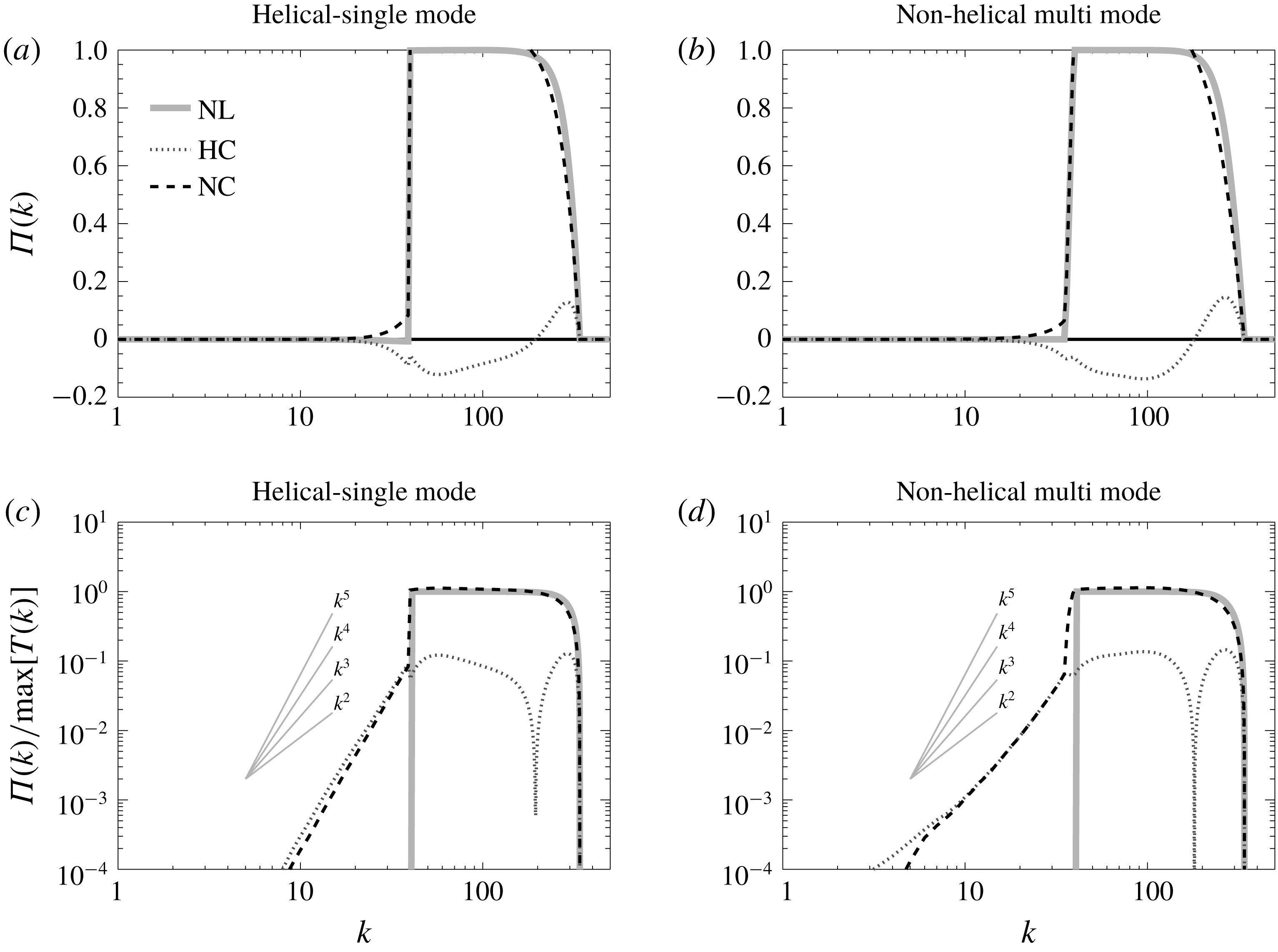
Decomposed fluxes using the helical decomposition for the flow HS0, (a,c), and the flow NM8 in (b,d). The index
 $HC$
stands for homochiral and
 $NC$
stands for non-homochiral (i.e. heterochiral). The total flux using the full nonlinear term is marked by NL. (a,b) are in linear–log scale while (c,d) show the absolute value in log–log scale.

Another direction for analysing the energy fluxes has been discussed recently and comes from decomposing the velocity field in helical modes (Craya Reference Craya1958; Lesieur Reference Lesieur1972; Herring Reference Herring1974). In this way every Fourier mode is written as the sum of two modes one with positive helicity and one with negative helicity
 $$\begin{eqnarray}\displaystyle \tilde{\boldsymbol{u}}_{\boldsymbol{k}}=\tilde{u} _{\boldsymbol{k}}^{+}\boldsymbol{h}_{\boldsymbol{k}}^{+}+\tilde{u} _{\boldsymbol{k}}^{-}\boldsymbol{h}_{\boldsymbol{k}}^{-}, & & \displaystyle\end{eqnarray}$$
where
 $\boldsymbol{h}_{\boldsymbol{k}}^{\pm }$
are eigenfunctions of the curl operator
 $\text{i}\boldsymbol{k}\times \boldsymbol{h}_{\boldsymbol{k}}^{\pm }=\pm k\boldsymbol{h}_{\boldsymbol{k}}^{\pm }$
(see appendix C). This decomposition splits the interactions among different modes into interactions that are homochiral (involve only modes with the same sign of helicity) or heterochiral (involve modes of both signs of helicity). Homochiral interactions tend to transfer on average energy to the large scales while heterochiral interactions tend to transfer energy on average to the small scales. This was first conjectured by Waleffe (Reference Waleffe1992) based on the stability properties of isolated triads, and has been discussed in may works (Waleffe Reference Waleffe1993; Chen, Chen & Eyink Reference Chen, Chen and Eyink2003; Moffatt Reference Moffatt2014; Rathmann & Ditlevsen Reference Rathmann and Ditlevsen2017). The homochiral interactions, when isolated so that the flow is driven only by them, lead to an inverse cascade (Biferale, Musacchio & Toschi Reference Biferale, Musacchio and Toschi2012, Reference Biferale, Musacchio and Toschi2013; Sahoo, Alexakis & Biferale Reference Sahoo, Alexakis and Biferale2017; Sahoo & Biferale Reference Sahoo and Biferale2018). In Alexakis (Reference Alexakis2017) it was also shown that even in non-helical turbulence the homochiral interactions, although sub-dominant, transfer energy inversely in the inertial range.
It is thus worth looking also the role played by homochiral and heterochiral interactions in the large-scale equilibrium situation. Following Alexakis (Reference Alexakis2017) we define the homochiral flux as
 $$\begin{eqnarray}\displaystyle \unicode[STIX]{x1D6F1}_{HC}(k)=\langle (\boldsymbol{u}^{+})^{{<}k}\boldsymbol{\cdot }(\boldsymbol{u}^{+}\boldsymbol{\cdot }\unicode[STIX]{x1D735}\boldsymbol{u}^{+})\rangle +\langle (\boldsymbol{u}^{-})^{{<}k}\boldsymbol{\cdot }(\boldsymbol{u}^{-}\boldsymbol{\cdot }\unicode[STIX]{x1D735}\boldsymbol{u}^{-})\rangle , & & \displaystyle\end{eqnarray}$$
and the heterochiral flux as
 $$\begin{eqnarray}\displaystyle \unicode[STIX]{x1D6F1}_{NC}(k)=\unicode[STIX]{x1D6F1}(k)-\unicode[STIX]{x1D6F1}_{HC}(k), & & \displaystyle\end{eqnarray}$$
where the vector fields
 $\boldsymbol{u}^{+}$
and
 $\boldsymbol{u}^{-}$
are defined as
 $$\begin{eqnarray}\displaystyle \boldsymbol{u}^{\pm }=\mathop{\sum }_{\boldsymbol{k}}\boldsymbol{h}_{\boldsymbol{k}}^{\pm }u_{k}^{\pm }\text{e}^{\text{i}\boldsymbol{k}\boldsymbol{x}}, & & \displaystyle\end{eqnarray}$$
and the
 ${<}k$
upper index stands for the filtering such that only Fourier modes of wavenumbers smaller than
 $k$
are retained as in (4.16).
In figure 12 the total flux
 $\unicode[STIX]{x1D6F1}(k)$
and the homochiral flux
 $\unicode[STIX]{x1D6F1}_{HC}(k)$
and heterochiral flux
 $\unicode[STIX]{x1D6F1}_{NC}(k)$
are shown for the same runs as in figure 11. Panels (a,b) are in linear–logarithmic scale while (c,d) are in log–log scale and display the absolute value. As shown in Alexakis (Reference Alexakis2017) the flux due to homochiral interactions is negative at almost all scales while the flux due to heterochiral interactions is positive. At the small turbulent scales the homochiral inverse flux is sub-dominant, while at the large scales the two counter-directed fluxes come in balance. At the large scales the two fluxes appear to follow a power law that is close to
 $k^{5}$
or
 $k^{4}$
for the six-mode forcing while it is closer to
 $k^{3}$
for the multi-mode forcing. A similar balance between homochiral and heterochiral interactions has also been observed at the large scales of rotating turbulence (Buzzicotti et al.
Reference Buzzicotti, Aluie, Biferale and Linkmann2018a
; Buzzicotti, Di Leoni & Biferale Reference Buzzicotti, Di Leoni and Biferale2018b
).
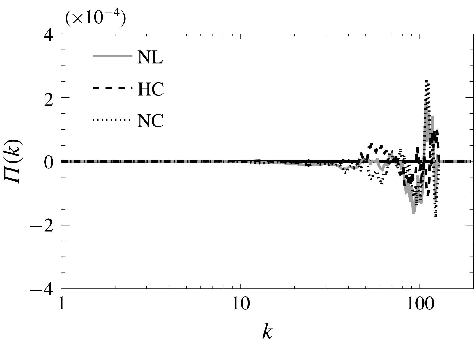
Homochiral and heterochiral fluxes for a truncated Euler equation system at thermal equilibrium.

We note that this organized inverse flux from the homochiral interactions does not appear in simulations of the truncated Euler equations in thermal equilibrium that result in zero net flux. This is demonstrated in figure 13 that shows the two fluxes
 $\unicode[STIX]{x1D6F1}_{HC}(k)$
and
 $\unicode[STIX]{x1D6F1}_{NC}(k)$
from a simulation of the truncated Euler equations. The two fluxes, although averaged over many outputs, appear noisy with no preferential direction of cascade. Thus the non-zero and sign-definite value of the fluxes
 $\unicode[STIX]{x1D6F1}_{HC}(k)$
and
 $\unicode[STIX]{x1D6F1}_{NC}(k)$
that was observed in the forced runs indicates a deviation from thermal equilibrium.
4.6 Energy shell to shell transfers
We end this section by examining the shell to shell transfer functions
 ${\mathcal{T}}(K,Q)$
that express the rate energy is transferred from one shell of wavenumbers
 $K<|\boldsymbol{k}|<K+1$
to another shell of wavenumbers
 $Q<|\boldsymbol{k}|<Q+1$
. We define these transfer functions as
 $$\begin{eqnarray}\displaystyle {\mathcal{T}}(K,Q)=-\langle \boldsymbol{u}_{K}(\boldsymbol{u}\boldsymbol{\cdot }\unicode[STIX]{x1D735})\boldsymbol{u}_{Q}\rangle , & & \displaystyle\end{eqnarray}$$
where
 $\boldsymbol{u}_{K}$
and
 $\boldsymbol{u}_{Q}$
are the velocity field filtered so that only the wavenumbers at shell
 $K$
and
 $Q$
are kept, respectively. These transfer functions have been studied extensively in the literature (Domaradzki & Rogallo Reference Domaradzki and Rogallo1990; Alexakis, Mininni & Pouquet Reference Alexakis, Mininni and Pouquet2005; Verma et al.
Reference Verma, Ayyer, Debliquy, Kumar and Chandra2005; Mininni, Alexakis & Pouquet Reference Mininni, Alexakis and Pouquet2006; Domaradzki & Carati Reference Domaradzki and Carati2007; Verma & Donzis Reference Verma and Donzis2007; Mininni et al.
Reference Mininni, Alexakis and Pouquet2008; Aluie & Eyink Reference Aluie and Eyink2009; Eyink & Aluie Reference Eyink and Aluie2009). If
 ${\mathcal{T}}(K,Q)<0$
it means that the shell
 $K$
is giving energy to the shell
 $Q$
while if
 ${\mathcal{T}}(K,Q)>0$
the shell
 $K$
is receiving energy from the shell
 $Q$
. The transfer
 ${\mathcal{T}}(K,Q)$
satisfies the relation
 ${\mathcal{T}}(K,Q)=-{\mathcal{T}}(Q,K)$
that reflects the conservation of energy by the nonlinear term.
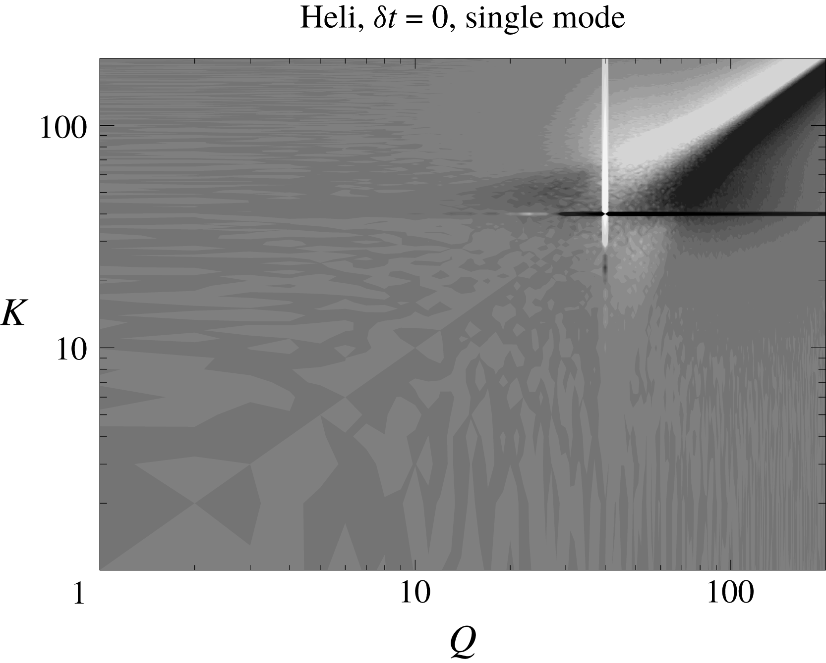
A grey scale image of the shell to shell transfer function
 ${\mathcal{T}}(K,Q)$
for a truncated Euler flow.

We calculate
 ${\mathcal{T}}(K,Q)$
for the truncated Euler flow and it is displayed in figure 14 where dark colours imply negative values of
 ${\mathcal{T}}(K,Q)$
, while light colours imply positive values. As expected for the thermal flows the transfer function appears as noise. This is because at the absolute equilibrium state there is no preferential direction of transfer of energy from any set of wavenumbers to any other. If averaged over many outputs
 ${\mathcal{T}}(K,Q)$
will become zero.
A grey scale image of the shell to shell transfer function
 ${\mathcal{T}}(K,Q)$
for the run HS0.

The situation is different when we investigate the flows obeying the forced Navier–Stokes equation. In figure 15 we plot the transfer function
 ${\mathcal{T}}(K,Q)$
for the flow HS0 (helical, six mode,
 $\unicode[STIX]{x1D6FF}t=0$
) that displayed a thermal energy spectrum at the large scales. The dark horizontal line at
 $K=k_{f}=40$
and the bright vertical line at
 $Q=k_{f}$
represent the transfer of energy from the forced modes that interact and transfer energy to almost all wavenumbers. For values of both
 $Q$
and
 $K$
larger than the forcing wavenumber;
 ${\mathcal{T}}(K,Q)$
displays the standard behaviour for the forward cascade with negative (dark) values below the diagonal
 $Q=K$
and positive values (light) above the diagonal, indicating that energy is transferred from the small wavenumbers to the large. For values of both
 $Q$
and
 $K$
smaller than the forcing wavenumber,
 ${\mathcal{T}}(K,Q)$
is almost zero. An exchange of energy with the large scales is observed only with the forcing scale (bright and dark lines at
 $Q=40$
and
 $K=40$
) that inject energy to the large scales, and some exchange (both positive and negative) with the turbulent scales indicated by the light and bright patches in the top left quadrant and bottom right quadrant.
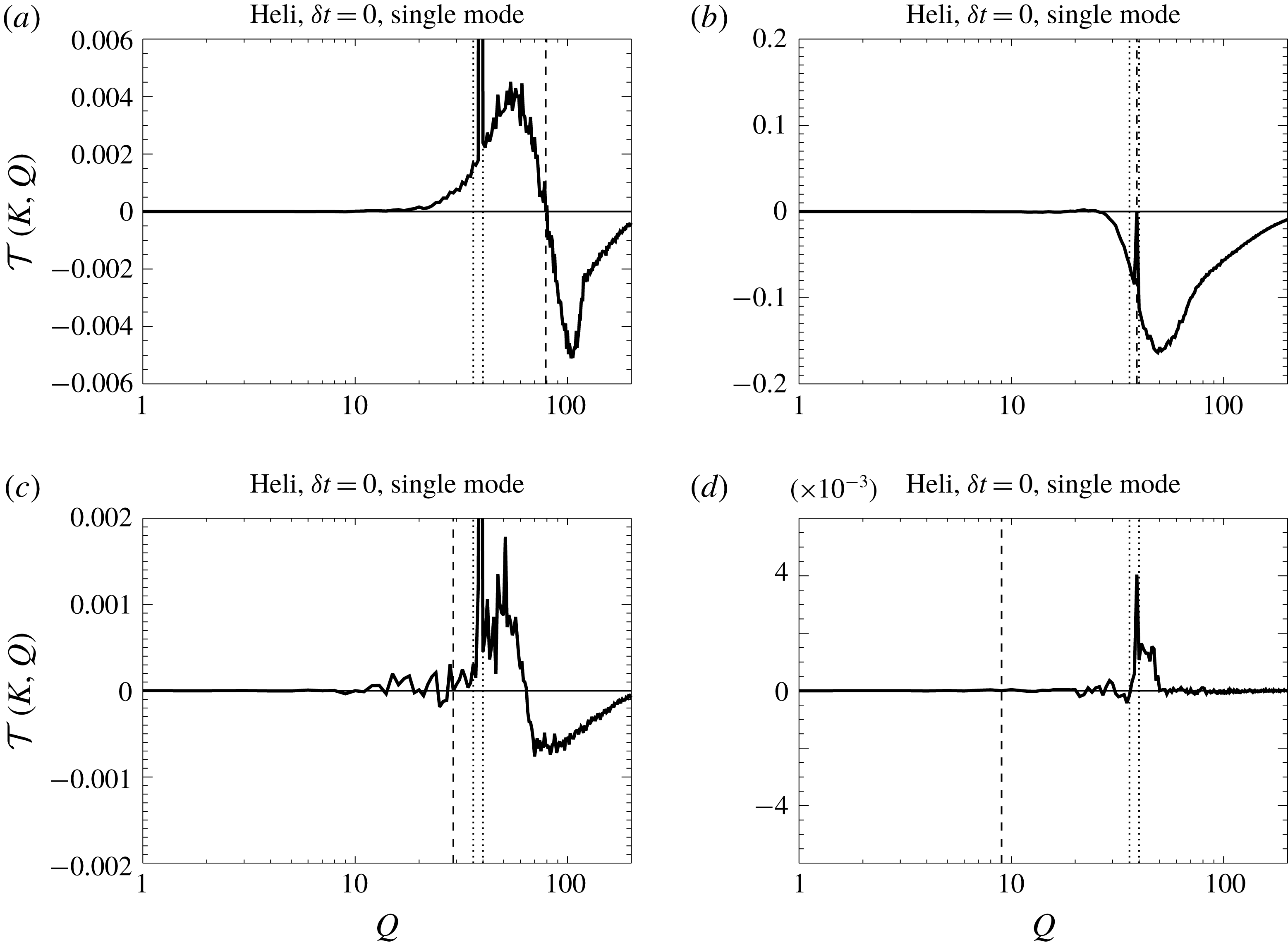
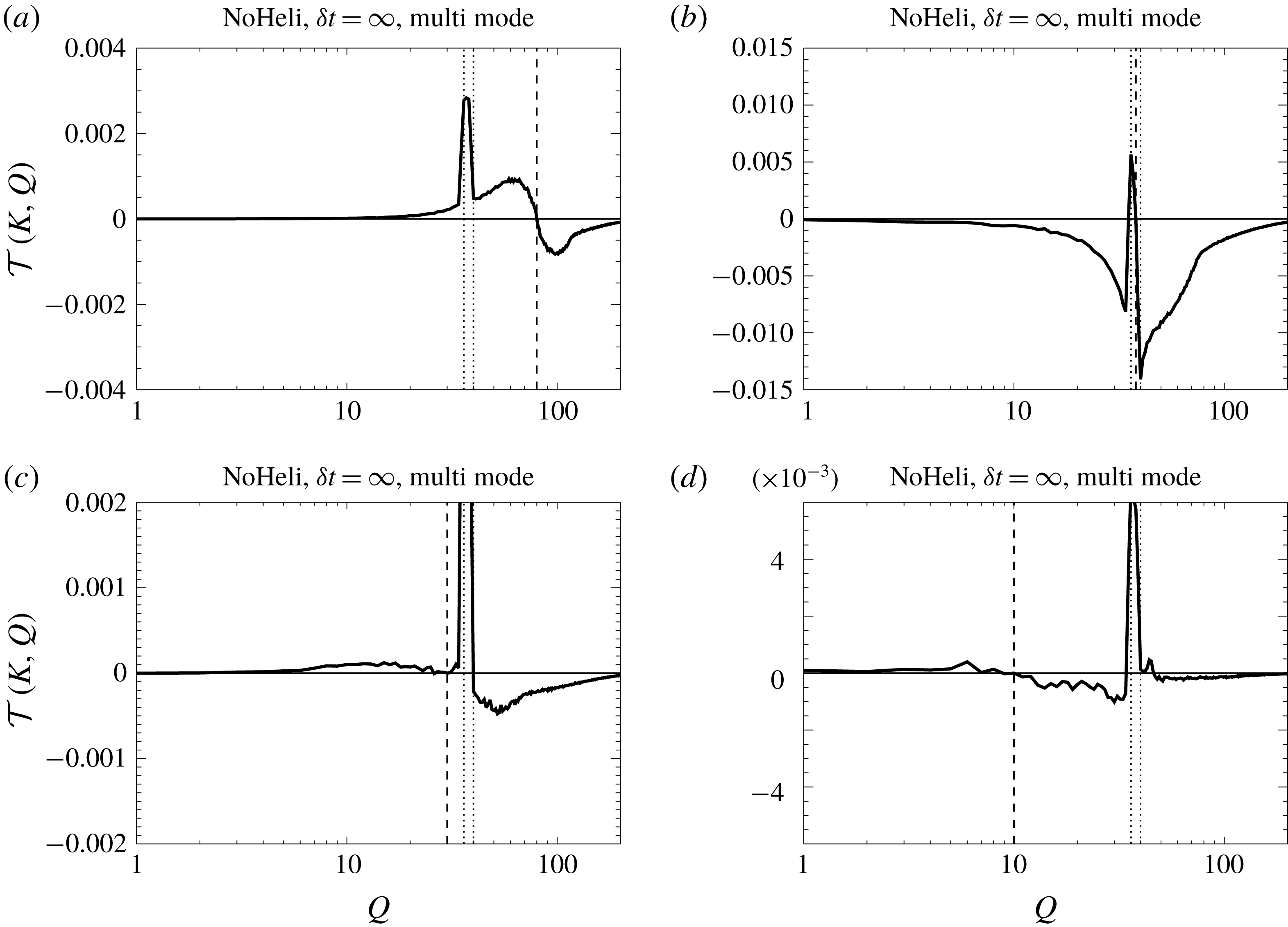
Shell to shell transfer function
 ${\mathcal{T}}(K,Q)$
as a function of
 $Q$
for four different values of (a–d)
 $K=80,40,30,10$
obtained from the flow HS0.

The transfers are displayed more clearly if we examine particular values of
 $K$
. In figure 16 we plot
 ${\mathcal{T}}(K,Q)$
as a function of
 $Q$
for
 $K=80,40,30,10$
. The value of
 $K$
is also indicated in (a–d) by the vertical dashed line, while the doted lines indicate the forcing scales. Positive values of
 ${\mathcal{T}}(K,Q)$
indicate the range of wavenumbers where the examined
 $K$
receives energy while negative values indicate the range of wavenumbers where it gives energy. The
 $K=80$
shell receives energy from all smaller wavenumbers
 $(Q<K)$
and gives energy to all larger wavenumbers
 $(Q>K)$
. The forcing scale
 $K=40$
gives energy to all wavenumbers small and large. The
 $K=30$
shell receives energy from the forcing scales while it loses energy to the largest wavenumbers
 $(Q>60)$
, and the largest scales
 $K=10$
only exchange energy with scales close to the forcing scales.
A grey scale image of the shell to shell transfer function
 ${\mathcal{T}}(K,Q)$
for the run NM8.

In figure 17 we plot the transfer function
 ${\mathcal{T}}(K,Q)$
for the flow NM8 (non-helical, multi-mode,
 $\unicode[STIX]{x1D6FF}t=\infty$
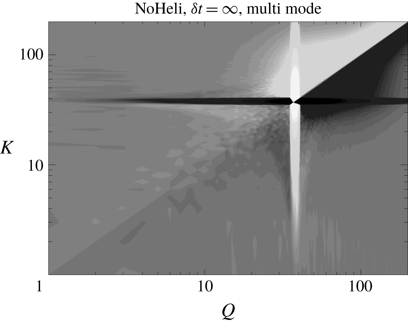
) that displayed strong deviations from the thermal energy spectrum at the large scales. The overall picture is similar to that of figure 15 although the interactions with the forcing scale are much more intense, and one can observe a local forward cascade at the large scales indicated by the bright region above the diagonal and dark region bellow the diagonal for
 $K,Q<k_{f}$
.
For more detail, in figure 18 we plot the transfer function
 ${\mathcal{T}}(K,Q)$
for the same wavenumbers
 $K$
as in figure 16. The overall picture for the turbulent and forced scales is the same as in 16 with larger scales giving energy to smaller scales and the forced scale giving energy to all. There are significant differences however if we look at the energy exchange at the large scales. At these scales there is a sign of a local forward cascade at large scales; the shell
 $K=10$
receives energy from smaller wavenumbers and gives energy to nearby larger wavenumbers. At the same time the same shell receives energy non-locally from the forcing scale and loses energy non-locally to the turbulent scales. This strengthens the picture from previous sections that when large scales are away from the thermal equilibrium due to an excess of energy from the forcing the large scales try to recover the thermal equilibrium by transporting (locally and non-locally) the energy to the smaller scales.
Shell to shell transfer function
 ${\mathcal{T}}(K,Q)$
as a function of
 $Q$
for four different values of (a–d)
 $K=80,40,30,10$
obtained from the flow NM8.

5 Summary and conclusions
The present work has examined 12 different simulated flows forced at small scales with a scope to understand better the behaviour of large scale flows and their relation to the absolute equilibrium solutions predicted by Kraichnan (Reference Kraichnan1973). The results were particularly interesting, revealing a variety of behaviours for the large-scale components of turbulent flows. In particular, it was shown in § 3 that the absolute equilibrium solutions are well reproduced by the large scales of turbulent flows when a few modes are forced (spectrally sparse forcing), and when the forcing of these modes is sufficiently short time correlated. Small deviations from the absolute equilibrium solutions were observed when the forcing correlation time was increased. Helicity did not play a significant role and even for a fully helical forcing function very little helicity was injected into the large scales, making the large-scale flows almost non-helical. Strong deviations from the absolute equilibrium solutions were observed when the forcing was applied to all modes inside a spherical shell (spectrally dense forcing). In this case, and particularly for the infinitely time correlated forcing, the power-law behaviour of the energy spectrum was far from the absolute equilibrium prediction
 $k^{2}$
and was closer to a
 $k$
independent behaviour.
The cause of this apparent lack of universality at the large scales was argued in § 4.1 to be due to the number of triads that couple a large-scale mode with two forced modes. In the first case of sparse forcing these triads were absent while for the spectrally dense forcing they were shown to follow a power-law distribution with the large-scale wavenumber
 $q$
that was
 $N_{Q}\propto q^{1}$
for
 $\unicode[STIX]{x1D6FF}k_{f}\ll q\ll k_{f}$
and
 $N_{Q}\propto q^{2}$
for
 $q\ll \unicode[STIX]{x1D6FF}k_{f}\ll k_{f}$
.
This difference altered the balance of the interactions at the large scales, something that was clearly reflected in the spectrum of the nonlinearity that was examined in § 4.2. The spectrally sparse forcing lead to a
 $k^{4}$
spectrum for the nonlinearity in agreement with the one calculated for flows in absolute equilibrium, while the spectrally dense forcing lead to a nonlinearity spectrum closer to
 $k^{3}$
which was in agreement with our estimates obtained assuming that the forced modes play a dominant role at the large scales. Decomposing the flow in § 4.3 into different components verified that for the sparse forcing the interactions that coupled two forced modes with one large-scale mode were absent, while for the spectrally dense forcing they were dominant and lead to a
 $k^{3}$
spectrum for the nonlinearity. The interactions with the forced modes in the latter case were shown to be balanced by the local large-scale interactions.
We further managed to identify the role played by the different scales by looking at the fluxes caused by different scales in § 4.4 and the shell-to-shell transfers in § 4.6. This analysis revealed that interactions with the forced scales inject energy to the large scales while interactions with the turbulent scales and large-scale self-interactions tend to bring energy back to the small scales. Finally, we investigated the fluxes due to homochiral and heterochiral interactions in § 4.5. The former were shown to move energy to the large scales while the latter moved energy away from the large scales in contrast with the absolute equilibrium flows for which these fluxes average to zero. The amplitude of these oppositely directed fluxes decreased as
 $q\rightarrow 0$
with a high power law.
Using a thermodynamics analogy the present analysis indicates that the large scales in a turbulent flow resemble a reservoir that is in a (non-local) contact with a second out-of-equilibrium reservoir consisting of the smaller (forced, turbulent and dissipative) scales. When the energy injection to the large scales from the forced modes is relatively weak (as is the case for the spectrally sparse forcing) then the large-scale spectrum remains close to a thermal equilibrium and the role of long-range interactions is to set the global energy (temperature) of the equilibrium state. If on the other hand the long-range interactions are dominant (as is the case for the spectrally dense forcing), the large-scale self-interactions cannot respond fast enough to bring the system into equilibrium and the large scales deviate from the equilibrium state and the energy spectrum can display different exponents.
We end by discussing the implications of our results for natural flows and decaying turbulence. In nature, flows are typically driven by instabilities. In such flows one can expect that scales larger than the typical instability length scale could also reach a thermal equilibrium state if the interactions with the instability modes are weak. If however the driving instability is such that has long correlation times and is dense in spectral space, deviations from the equilibrium state can be expected. Our work also indicates that caution needs to be taken in systems that transition from forward to an inverse cascade. Flows that show strong deviations from the thermal equilibrium lead to an excess of energy input at the large scales even if no inverse cascade is present. Such an excess of energy can easily be mistaken for a weak inverse cascade if the system is not run long enough so that a steady state is established. Finally we note that although the large scales in forced turbulence and decaying turbulence can have similar spectra, the underlaying mechanisms can be very different. In forced turbulence the large scales are being controlled to a large extent by the forced modes and it is their density in spectral space and time correlation that determine their properties. In decaying turbulence there are no forced modes and the fate of the large scales is determined by the initial conditions. One could however imagine that, at least for short times, initial conditions that are spectrally dense could have different behaviour than initial conditions that are spectrally sparse. Further numerical and experimental studies could shed light on these issues.
Acknowledgements
The authors acknowledge insightful discussions with S. Fauve, S. Perrard and G. Prabhudesai. This work was granted access to the HPC resources of MesoPSL financed by the Region Ile de France and the project Equip@Meso (reference ANR-10-EQPX-29-01) of the programme Investissements d’Avenir supervised by the Agence Nationale pour la Recherche and the HPC resources of GENCI-TGCC and GENCI-CINES (project nos A0010506421, A0030506421 and A0050506421) where the present numerical simulations have been performed. This work has also been supported by the Agence nationale de la recherche (ANR DYSTURB project no. ANR-17-CE30-0004).
Appendix A. Number of interacting triads
For a given mode
 $\boldsymbol{q}$
, the number of modes
 $\boldsymbol{k}_{1},\boldsymbol{k}_{2}\in K_{F}$
that satisfy
 $\boldsymbol{q}+\boldsymbol{k}_{1}+\boldsymbol{k}_{2}=0$
is given by the number of modes
 $N_{\boldsymbol{q}}$
that reside in the intersection of the two spherical shells
 $k_{f}-\unicode[STIX]{x1D6FF}k_{f}<|\boldsymbol{k}|\leqslant k_{f}$
and
 $k_{f}-\unicode[STIX]{x1D6FF}k_{f}<|\boldsymbol{k}+\boldsymbol{q}|\leqslant k_{f}$
. Since the density of wavenumbers in the Fourier space for a cubic domain of side
 $2\unicode[STIX]{x03C0}$
is uniform and equal to unity
 $N_{\boldsymbol{q}}$
is approximately equal to the volume of the aforementioned intersection (it becomes exactly equal to
 $N_{\boldsymbol{q}}$
when
 $k_{f}\rightarrow \infty$
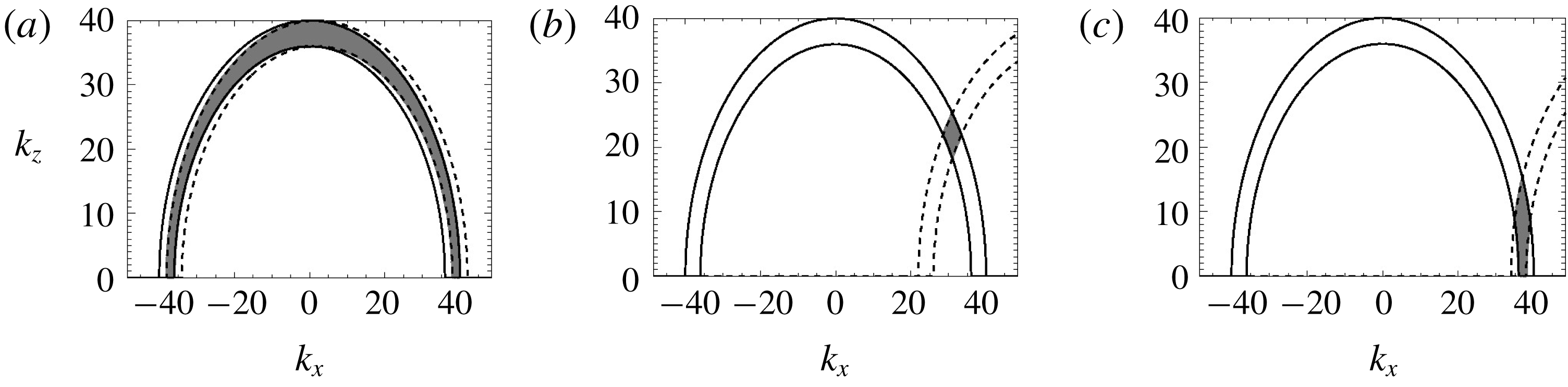
). This intersection for three different values of
 $\boldsymbol{q}=(q,0,0)$
is demonstrated in figure 19. Note that in figure 19 only a plane cut is shown at
 $k_{y}=0$
but the intersection area is symmetric around the axis of
 $\boldsymbol{q}$
here taken to be the
 $x$
-axis.
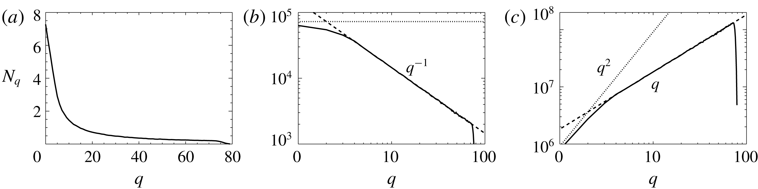
The volume of the intersection can be easily calculated (e.g. by a Monte Carlo method) the results of which for our case (
 $k_{f}=40$
and
 $\unicode[STIX]{x1D6FF}k_{f}=4$
) are shown in figure 20 in linear scale (a) and a log–log scale in (b). It results in a
 $q^{-1}$
power-law behaviour for
 $\unicode[STIX]{x1D6FF}k_{f}\ll q\ll k_{f}$
. This power law can easily be predicted by noting that in this range of
 $q$
the intersection volume is given by
 $N_{\boldsymbol{q}}=2\unicode[STIX]{x03C0}A(k_{f}^{2}-q^{2})^{1/2}$
, where
 $A$
is the area of the small rectangle shown more clearly in figure 19(b), and rotational symmetry around
 $\boldsymbol{q}$
has been taken into account. This area
 $A$
is given by
 $A=\unicode[STIX]{x1D6FF}k_{f}^{2}/\sin (2\unicode[STIX]{x1D703})$
where
 $\unicode[STIX]{x1D703}=\arccos (q/k_{f})$
the angle formed by
 $\boldsymbol{k}$
and
 $\boldsymbol{q}$
. This leads to the prediction
 $$\begin{eqnarray}\displaystyle N_{\boldsymbol{q}}\simeq 2\unicode[STIX]{x03C0}k_{f}^{2}\unicode[STIX]{x1D6FF}k_{f}^{2}/q,\quad \text{for }\unicode[STIX]{x1D6FF}k_{f}\ll q\ll k_{f} & & \displaystyle\end{eqnarray}$$
which is the dashed line shown in figure 20(b). Then the total number of triads
 $N_{Q}$
having two modes in the forced shell and one mode in a spherical shell
 $Q$
of unit width and of radius
 $q$
, is given by
 $N_{Q}=4\unicode[STIX]{x03C0}q^{2}N_{q}\simeq 8\unicode[STIX]{x03C0}^{2}k_{f}^{2}\unicode[STIX]{x1D6FF}k_{f}^{2}q$
, where the last equality holds for
 $\unicode[STIX]{x1D6FF}k_{f}\ll q\ll k_{f}$
. This number
 $N_{Q}$
is plotted in figure 20(c) (solid line) along with the approximation (dashed line).
The figure demonstrates how to calculate the number of triads that can be constructed with two modes inside the forcing shell and a large-scale mode
 $\boldsymbol{q}$
, for three different values of
 $|\boldsymbol{q}|=2$
(a)
 $|\boldsymbol{q}|=64$
(b) and
 $|\boldsymbol{q}|=74$
(c). The solid lines indicate the modes with
 $|\boldsymbol{k}|=k_{f}$
and
 $k_{f}-\unicode[STIX]{x1D6FF}k_{f}$
while the dashed lines indicate the circles
 $|\boldsymbol{k}+\boldsymbol{q}|=k_{f}$
and
 $k_{f}-\unicode[STIX]{x1D6FF}k_{f}$
. The modes
 $\boldsymbol{k}$
for which both
 $\boldsymbol{k}$
and
 $\boldsymbol{k}+\boldsymbol{q}$
are among the forced modes are given by the modes that lie in the intersection of the two spherical shells that is depicted by the shaded area. Note that almost all forcing modes can form triads with small
 $\boldsymbol{q}$
, while the allowed number of modes goes to zero when
 $|\boldsymbol{q}|=k_{f}$
.

(a) Number of interacting triads
 $N_{\boldsymbol{q}}$
between two forced modes (
 $|\boldsymbol{k}|\in [k_{f}-\unicode[STIX]{x1D6FF}k_{f},k_{f}]$
and a single large-scale mode
 $\boldsymbol{q}$
as a function of it modulus
 $q=|\boldsymbol{q}|$
. (b) Same plot in a log–log scale. The dashed line indicates the power law
 $q^{-1}$
. (c) Number of interacting triads of the forcing modes with all modes within a sphere of radius
 $q$
. The dashed lines indicate the asymptotic predictions
 $N_{\boldsymbol{q}}=2\unicode[STIX]{x03C0}k_{f}^{2}\unicode[STIX]{x1D6FF}k_{f}^{2}/q$
and
 $N_{Q}=8\unicode[STIX]{x03C0}^{2}k_{f}^{2}\unicode[STIX]{x1D6FF}k_{f}^{2}q$
(see (A 1)), while the doted lines indicate the prediction for
 $q\rightarrow 0$
(see (A 2)).

For
 $q\ll \unicode[STIX]{x1D6FF}k_{f}$
the number
 $N_{q}$
approaches a finite value that corresponds to the case that the two spherical shells overlap. Thus for
 $q\ll \unicode[STIX]{x1D6FF}k_{f}\ll k_{f}$
the number of interacting triads is equal to the volume of the spherical shell
 $$\begin{eqnarray}\displaystyle N_{\boldsymbol{q}}=4\unicode[STIX]{x03C0}k_{f}^{2}\unicode[STIX]{x1D6FF}k_{f}\quad \text{for }q\ll \unicode[STIX]{x1D6FF}k_{f}\ll k_{f}, & & \displaystyle\end{eqnarray}$$
shown by the horizontal dotted line in figure 20(b). The total number of interacting triads with all modes in the spherical shell of radius between
 $q$
and
 $q+1$
is
 $N_{Q}=16\unicode[STIX]{x03C0}^{2}q^{2}k_{f}^{2}\unicode[STIX]{x1D6FF}k_{f}$
. Note that for
 $\unicode[STIX]{x1D6FF}k_{f}\ll q$
we have
 $N_{Q}\propto q$
while for
 $q\ll \unicode[STIX]{x1D6FF}k_{f}$
we have
 $N_{Q}\propto q^{2}$
.
Appendix B. Nonlinearity spectrum and pressure spectrum for flows in absolute equilibrium
Using the Fourier transform of the velocity field
 $\boldsymbol{v}(\boldsymbol{x},t)=\sum \hat{\boldsymbol{v}}(\boldsymbol{k},t)\text{e}^{\text{i}\boldsymbol{k}\boldsymbol{\cdot }\boldsymbol{x}}$
, the truncated Euler equations (1.1) can be expressed as the finite system of ordinary differential equations for the complex variables
 $\hat{\boldsymbol{v}}(\boldsymbol{k})$
 $$\begin{eqnarray}\displaystyle \unicode[STIX]{x2202}_{t}\hat{v}_{\unicode[STIX]{x1D6FC}}(\boldsymbol{k},t)=-\frac{\text{i}}{2}{\mathcal{P}}_{\unicode[STIX]{x1D6FC}\unicode[STIX]{x1D6FD}\unicode[STIX]{x1D6FE}}(\boldsymbol{k})\mathop{\sum }_{\boldsymbol{p}}\hat{v}_{\unicode[STIX]{x1D6FD}}(\boldsymbol{p},t)\hat{v}_{\unicode[STIX]{x1D6FE}}(\boldsymbol{k}-\boldsymbol{p},t) & & \displaystyle\end{eqnarray}$$
where
 ${\mathcal{P}}_{\unicode[STIX]{x1D6FC}\unicode[STIX]{x1D6FD}\unicode[STIX]{x1D6FE}}=k_{\unicode[STIX]{x1D6FD}}P_{\unicode[STIX]{x1D6FC}\unicode[STIX]{x1D6FE}}+k_{\unicode[STIX]{x1D6FE}}P_{\unicode[STIX]{x1D6FC}\unicode[STIX]{x1D6FD}}$
with
 $P_{\unicode[STIX]{x1D6FC}\unicode[STIX]{x1D6FD}}=\unicode[STIX]{x1D6FF}_{\unicode[STIX]{x1D6FC}\unicode[STIX]{x1D6FD}}-k_{\unicode[STIX]{x1D6FC}}k_{\unicode[STIX]{x1D6FD}}/k^{2}$
and the convolution in (B 1) is truncated to
 $\boldsymbol{k}^{2}\leqslant k_{max}^{2}$
,
 $\boldsymbol{p}^{2}\leqslant k_{max}^{2}$
and
 $(\boldsymbol{k}-\boldsymbol{p})^{2}\leqslant k_{max}^{2}$
.
Denoting by
 $\boldsymbol{f}(\boldsymbol{k})$
the right-hand side of (B 1), one has
 $$\begin{eqnarray}\displaystyle \langle f_{\unicode[STIX]{x1D6FC}}(\boldsymbol{k})f_{\unicode[STIX]{x1D6FF}}(\boldsymbol{k}^{\prime })\rangle =-\frac{1}{4}{\mathcal{P}}_{\unicode[STIX]{x1D6FC}\unicode[STIX]{x1D6FD}\unicode[STIX]{x1D6FE}}(\boldsymbol{k}){\mathcal{P}}_{\unicode[STIX]{x1D6FF}\unicode[STIX]{x1D707}\unicode[STIX]{x1D708}}(\boldsymbol{k}^{\prime })\mathop{\sum }_{\boldsymbol{ p}}\mathop{\sum }_{\boldsymbol{p}^{\prime }}\langle \hat{v}_{\unicode[STIX]{x1D6FD}}(\boldsymbol{p})\hat{v}_{\unicode[STIX]{x1D6FE}}(\boldsymbol{k}-\boldsymbol{p})\hat{v}_{\unicode[STIX]{x1D707}}(\boldsymbol{p}^{\prime })\hat{v}_{\unicode[STIX]{x1D708}}(\boldsymbol{k}^{\prime }-\boldsymbol{p}^{\prime })\rangle , & & \displaystyle\end{eqnarray}$$
where here
 $\langle \cdot \rangle$
denotes the (ensemble) average is taken over the absolute equilibrium which is a zero-mean Gaussian field with second-order moment given by (see e.g. Orszag (Reference Orszag, Balian and Peube1977), (5–16))
 $$\begin{eqnarray}\displaystyle \langle \hat{v}_{\unicode[STIX]{x1D6FC}}(\boldsymbol{k}_{1},t)\hat{v}_{\unicode[STIX]{x1D6FD}}(\boldsymbol{k}_{2},t)\rangle =CP_{\unicode[STIX]{x1D6FC}\unicode[STIX]{x1D6FD}}(\boldsymbol{k})\unicode[STIX]{x1D6FF}(\boldsymbol{k}_{1}+\boldsymbol{k}_{2}) & & \displaystyle\end{eqnarray}$$
for
 $\boldsymbol{k}^{2}\leqslant k_{max}^{2}$
. Using the standard expression for fourth-order moment zero-mean jointly Gaussian random variables with covariance
 $\unicode[STIX]{x1D6E4}_{ij}$
(see e.g. Frisch (Reference Frisch1995), equation (4–21))
 $$\begin{eqnarray}\displaystyle \langle v_{1}v_{2}v_{3}v_{4}\rangle =\unicode[STIX]{x1D6E4}_{12}\unicode[STIX]{x1D6E4}_{34}+\unicode[STIX]{x1D6E4}_{13}\unicode[STIX]{x1D6E4}_{24}+\unicode[STIX]{x1D6E4}_{14}\unicode[STIX]{x1D6E4}_{23}. & & \displaystyle\end{eqnarray}$$
Two of the terms in (B 4) are equal while the third is zero, yielding
 $$\begin{eqnarray}\displaystyle \langle f_{\unicode[STIX]{x1D6FC}}(\boldsymbol{k})f_{\unicode[STIX]{x1D6FF}}(-\boldsymbol{k})\rangle =-\mathop{\sum }_{\boldsymbol{q}}\frac{C^{2}}{2}{\mathcal{P}}_{\unicode[STIX]{x1D6FC}\unicode[STIX]{x1D6FD}\unicode[STIX]{x1D6FE}}(\boldsymbol{k}){\mathcal{P}}_{\unicode[STIX]{x1D6FF}\unicode[STIX]{x1D707}\unicode[STIX]{x1D708}}(-\boldsymbol{k})P_{\unicode[STIX]{x1D6FD}\unicode[STIX]{x1D707}}(\boldsymbol{k}/2-\boldsymbol{q})P_{\unicode[STIX]{x1D6FE}\unicode[STIX]{x1D708}}(\boldsymbol{k}/2+\boldsymbol{q}). & & \displaystyle\end{eqnarray}$$
Setting
 $\boldsymbol{k}=(k,0,0)$
and
 $\boldsymbol{q}=(q_{x},q_{y},q_{z})$
, straightforward computation gives
 $$\begin{eqnarray}\langle f_{\unicode[STIX]{x1D6FC}}(\boldsymbol{k})f_{\unicode[STIX]{x1D6FC}}(-\boldsymbol{k})\rangle =\frac{4C^{2}k_{x}^{2}(q_{y}^{2}+q_{z}^{2})(k_{x}^{2}+4(3q_{x}^{2}+q_{y}^{2}+q_{z}^{2}))}{(k_{x}^{2}-4k_{x}q_{x}+4(q_{x}^{2}+q_{y}^{2}+q_{z}^{2}))(k_{x}^{2}+4k_{x}q_{x}+4(q_{x}^{2}+q_{y}^{2}+q_{z}^{2}))}.\end{eqnarray}$$
For large
 $k_{max}$
, setting
 $(q_{x},q_{y},q_{z})=(xk_{max},yk_{max},zk_{max})$
and taking the dominant term in the limit
 $\unicode[STIX]{x1D716}=k/k_{max}\rightarrow 0$
, the integral over
 $(x,y,z)$
performed in polar coordinates, yields
 $$\begin{eqnarray}\displaystyle \langle f_{\unicode[STIX]{x1D6FC}}(\boldsymbol{k})f_{\unicode[STIX]{x1D6FC}}(-\boldsymbol{k})\rangle ={\textstyle \frac{56}{45}}\unicode[STIX]{x03C0}C^{2}k_{max}^{3}k^{2}. & & \displaystyle\end{eqnarray}$$
The variable
 $C$
in (B 3) can be related to the total thermalized energy
 ${\mathcal{E}}$
by
 ${\mathcal{E}}=\sum _{k\leqslant k_{max}}E(k)=(C/2)\sum _{|\boldsymbol{k}|\leqslant k_{max}}P_{\unicode[STIX]{x1D6FC}\unicode[STIX]{x1D6FC}}(\boldsymbol{k})=C(4/3)\unicode[STIX]{x03C0}k_{max}^{3}$
. Thus, the thermal energy spectrum reads
 $$\begin{eqnarray}\displaystyle E(k)=3{\mathcal{E}}\frac{k^{2}}{k_{max}^{3}}, & & \displaystyle\end{eqnarray}$$
and one finally finds for the spectrum
 $E_{{\mathcal{N}}}(k)=4\unicode[STIX]{x03C0}k^{2}<f_{\unicode[STIX]{x1D6FC}}(\boldsymbol{k})f_{\unicode[STIX]{x1D6FC}}(-\boldsymbol{k})>$
of the nonlinear term
 $$\begin{eqnarray}\displaystyle E_{{\mathcal{N}}}(k)={\textstyle \frac{14}{15}}{\mathcal{E}}k^{2}E(k). & & \displaystyle\end{eqnarray}$$
A similar computation, starting with (B 1) but keeping only the gradient terms in
 ${\mathcal{P}}_{\unicode[STIX]{x1D6FC}\unicode[STIX]{x1D6FD}\unicode[STIX]{x1D6FE}}$
yields for the pressure gradient spectrum
 $E_{PG}(k)=(16/15){\mathcal{E}}k^{2}E(k)$
.
The pressure spectrum is thus given by
 $$\begin{eqnarray}\displaystyle E_{P}(k)={\textstyle \frac{16}{15}}{\mathcal{E}}E(k). & & \displaystyle\end{eqnarray}$$
Appendix C. Spectrum of the nonlinearity for forced flows
We can estimate the spectrum of the nonlinearity for small wavenumbers
 $\boldsymbol{q}$
if some further simplifications are made. We begin by expressing the nonlinearity in terms of the helical mode decomposition. In three dimensions, the three components of the Fourier modes
 $\tilde{\boldsymbol{u}}_{k}$
satisfy the incompressibility condition
 $\tilde{\boldsymbol{u}}_{k}\boldsymbol{\cdot }k=0$
leaving two independent complex amplitudes. Therefore each Fourier mode can be further decomposed into two modes. From all possible basis that a Fourier mode of an incompressible field can be decomposed the most fruitful perhaps has been that of the decomposition to two helical modes (Craya Reference Craya1958; Lesieur Reference Lesieur1972; Herring Reference Herring1974). This has been used in many classical papers (Constantin & Majda Reference Constantin and Majda1988; Cambon & Jacquin Reference Cambon and Jacquin1989; Waleffe Reference Waleffe1992). In this decomposition a Fourier mode
 $\tilde{\boldsymbol{u}}_{k}$
of the velocity field is written as
 $$\begin{eqnarray}\displaystyle \tilde{\boldsymbol{u}}_{\boldsymbol{k}}=\tilde{u} _{\boldsymbol{k}}^{+}\boldsymbol{h}_{\boldsymbol{k}}^{+}+\tilde{u} _{\boldsymbol{k}}^{-}\boldsymbol{h}_{\boldsymbol{k}}^{-}, & & \displaystyle\end{eqnarray}$$
where the basis vectors
 $\boldsymbol{h}_{\boldsymbol{k}}^{+},\boldsymbol{h}_{\boldsymbol{k}}^{-}$
are
 $$\begin{eqnarray}\displaystyle \boldsymbol{h}_{\boldsymbol{k}}^{s}=\frac{\boldsymbol{k}\times (\boldsymbol{e}\times \boldsymbol{k})}{\sqrt{2}|\boldsymbol{k}\times (\boldsymbol{e}\times \boldsymbol{k})|}+\text{i}s\frac{\boldsymbol{e}\times \boldsymbol{k}}{\sqrt{2}|\boldsymbol{e}\times \boldsymbol{k}|}. & & \displaystyle\end{eqnarray}$$
Here
 $\boldsymbol{e}$
is an arbitrary unit vector. The sign index
 $s=\pm 1$
indicates the sign of the helicity of
 $\boldsymbol{h}_{\boldsymbol{k}}^{s}$
. The basis vectors
 $\boldsymbol{h}_{\boldsymbol{k}}^{s}$
are eigenfunctions of the curl operator in Fourier space such that
 $\text{i}\boldsymbol{k}\times \boldsymbol{h}_{\boldsymbol{k}}^{s}=s|\boldsymbol{k}|\boldsymbol{h}_{\boldsymbol{k}}^{s}$
and satisfy
 $\boldsymbol{h}_{\boldsymbol{k}}^{s}\boldsymbol{\cdot }\boldsymbol{h}_{\boldsymbol{k}}^{s}=0$
and
 $\boldsymbol{h}_{\boldsymbol{k}}^{s}\boldsymbol{\cdot }\boldsymbol{h}_{\boldsymbol{k}}^{-s}=\boldsymbol{h}_{\boldsymbol{k}}^{s}\boldsymbol{\cdot }\boldsymbol{h}_{-\boldsymbol{k}}^{s}=1$
and form a complete base for incompressible vector fields. The nonlinearity that acts on a mode
 $\tilde{u} _{\boldsymbol{q}}^{s_{\boldsymbol{q}}}$
is given by (see Cambon & Jacquin (Reference Cambon and Jacquin1989), Waleffe (Reference Waleffe1992))
 $$\begin{eqnarray}\displaystyle \tilde{{\mathcal{N}}}^{s_{\boldsymbol{q}}}(\boldsymbol{q})=h_{-\boldsymbol{q}}^{s_{q}}\boldsymbol{\cdot }\tilde{{\mathcal{N}}}(\boldsymbol{q})=\mathop{\sum }_{\boldsymbol{q}=\boldsymbol{p}+\boldsymbol{k}}\mathop{\sum }_{s_{\boldsymbol{k}},s_{\boldsymbol{p}}}C_{\boldsymbol{q},\boldsymbol{k},\boldsymbol{p}}^{s_{\boldsymbol{q}},s_{\boldsymbol{k}},s_{\boldsymbol{p}}}u_{\boldsymbol{ k}}^{s_{\boldsymbol{k}}}u_{\boldsymbol{ p}}^{s_{\boldsymbol{p}}}, & & \displaystyle\end{eqnarray}$$
where the pre-factor
 $C_{\boldsymbol{q},\boldsymbol{k},\boldsymbol{p}}^{s_{\boldsymbol{q}},s_{\boldsymbol{k}},s_{\boldsymbol{p}}}$
is given by
 $$\begin{eqnarray}\displaystyle C_{\boldsymbol{q},\boldsymbol{k},\boldsymbol{p}}^{s_{\boldsymbol{q}},s_{\boldsymbol{k}},s_{\boldsymbol{p}}}={\textstyle \frac{1}{2}}(s_{\boldsymbol{k}}k-s_{\boldsymbol{p}}p)[h_{-\boldsymbol{q}}^{s_{q}}\boldsymbol{\cdot }(h_{\boldsymbol{ k}}^{s_{\boldsymbol{k}}}\times h_{\boldsymbol{ p}}^{s_{\boldsymbol{p}}})]. & & \displaystyle\end{eqnarray}$$
For
 $q\ll k$
we have that
 $p\simeq k(1-\boldsymbol{q}\boldsymbol{\cdot }\boldsymbol{k}/k^{2})$
and
 $h_{\boldsymbol{p}}^{s_{\boldsymbol{p}}}\simeq h_{-\boldsymbol{k}}^{s_{\boldsymbol{p}}}+\boldsymbol{q}\boldsymbol{\cdot }\unicode[STIX]{x2202}_{\boldsymbol{p}}h_{\boldsymbol{p}}^{s_{\boldsymbol{p}}}|_{\boldsymbol{p}=-\boldsymbol{k}}+O(q^{2})$
. This implies that if
 $s_{\boldsymbol{k}}=s_{\boldsymbol{p}}$
we would have
 $(s_{\boldsymbol{k}}k-s_{\boldsymbol{p}}p)\simeq s_{\boldsymbol{k}}\boldsymbol{q}\boldsymbol{\cdot }\boldsymbol{k}/k=O(q)$
. On the other hand if
 $s_{\boldsymbol{k}}=-s_{\boldsymbol{p}}$
we have that
 $(h_{\boldsymbol{k}}^{s_{\boldsymbol{k}}}\times h_{\boldsymbol{ p}}^{s_{\boldsymbol{p}}})=O(q)$
. In both cases we thus have that for
 $q\ll k$
 $$\begin{eqnarray}\displaystyle C_{\boldsymbol{q},\boldsymbol{k},\boldsymbol{p}}^{s_{\boldsymbol{q}},s_{\boldsymbol{k}},s_{\boldsymbol{p}}}=cq+O(q^{2}), & & \displaystyle\end{eqnarray}$$
where
 $c$
is an order-one coefficient independent of the amplitude of
 $q$
. If we sum over all triads assuming that the modes
 $u_{\boldsymbol{k}}^{s_{\boldsymbol{k}}}$
and
 $u_{\boldsymbol{p}}^{s_{\boldsymbol{p}}}$
are independent and randomly distributed we then obtain the estimate
 $$\begin{eqnarray}\displaystyle \tilde{{\mathcal{N}}}(\boldsymbol{q})\propto qu_{rms}^{2}\sqrt{N_{\boldsymbol{q}}}. & & \displaystyle\end{eqnarray}$$
Here
 $N_{\boldsymbol{q}}$
is the number of allowed triads and the square root is taken because have summed over
 $N_{\boldsymbol{q}}$
terms that take both negative and positive values. With
 $u_{rms}$
we denote the root mean square amplitude of a mode inside the spherical shell
 $K$
, that is proportional the energy spectrum
 $u_{rms}^{2}\propto E(k)/k^{2}dk$
. In writing equation (C 6) we assumed that no further dependence on
 $q$
comes due to phase alignment between the modes
 $u_{\boldsymbol{k}}^{s_{\boldsymbol{k}}}$
and
 $u_{\boldsymbol{p}}^{s_{\boldsymbol{p}}}$
. This is a good assumption if the flow is in thermal equilibrium and this estimate can become more precise. However, it is not in general a good assumption for the turbulent scales and as we shall see differences can be present. Squaring and summing over the
 $4\unicode[STIX]{x03C0}q^{2}dq$
modes inside a spherical shell of radius
 $q$
and width
 $dq$
we obtain
 $$\begin{eqnarray}\displaystyle E_{{\mathcal{N}}}(q)\propto q^{4}u_{rms}^{2}N_{q}. & & \displaystyle\end{eqnarray}$$
For a general flow however
 $E_{{\mathcal{N}}}(q)$
will depend on the shape of the energy spectrum
 $E(k)$
and on the possible phase alignments of all involved modes. As was shown in the previous section, if the shell of interacting wavenumbers is such that
 $q\ll dk$
then
 $N_{q}$
is independent of
 $q$
while if it is such that
 $q\ll dk$
then
 $N_{q}\propto 1/q$
. This implies the following for an arbitrary energy spectrum
 $E(k)$
that varies with
 $k$
from 0 to
 $\infty$
. If the energy spectrum is smooth (for variations
 $dk\gg q$
) then the interactions can be considered as the sum of interactions with different shells of width
 $dk\gg q$
that cover all
 $k$
-space. This will result in
 $E_{N}(q)\propto q^{4}$
. If however there is a strong peak (e.g. at the forcing scale) of the energy spectrum that occurs over a variation of
 $k$
by
 $dk\ll q$
then the interactions with this peak should follow
 $E_{N}(q)\propto q^{3}$
and could dominate the nonlinearity spectrum if the peak is strong enough.