





1 Introduction
Item parameter drift (IPD) refers to the systematic changes in item parameters over time (Kürşad et al., Reference Kürşad, Çokluk-bökeoglu and Çıkrıkçı2022; Zheng & Chang, Reference Zheng and Chang2017) and typically arises from instructional shifts or repeated item exposure (Guo et al., Reference Guo, Robin and Dorans2017; Lee & Lewis, Reference Lee and Lewis2021). When IPD occurs, it threatens measurement invariance and fairness, particularly in computerized adaptive testing (CAT), where items are repeatedly administered and tests are tailored in real time to each examinee’s ability level (Chang, Reference Chang2015; Wells et al., Reference Wells, Subkoviak and Serlin2002). The prevailing paradigm in most IPD detection research and practice relies on post hoc analyses of periodically collected data, which often fail to identify subtle and ongoing parameter changes in a timely manner, allowing compromised items to persist in the item bank and affect ability estimates long after drift has begun (Guo et al., Reference Guo, Zheng and Chang2015; Kang & Chang, Reference Kang and Chang2016; Lee & Lewis, Reference Lee and Lewis2021).
To address this limitation, online calibration methods have emerged as a promising alternative (Chen et al., Reference Chen, Xin, Wang and Chang2012; Kang et al., Reference Kang, Zheng and Chang2020; Zheng & Chang, Reference Zheng and Chang2017). By re-estimating item parameters concurrently with operational test administration, online calibration enables dynamic adjustment of sampling plans and facilitates the prompt detection of IPD as it emerges, thereby proactively safeguarding measurement quality (Chen & Wang, Reference Chen and Wang2016; He & Chen, Reference He and Chen2020; Kang, Reference Kang2023; Ren et al., Reference Ren, van der Linden and Diao2017). Within this framework, cumulative sum (CUSUM) control charts, which originate in the field of statistical process control, have proven effective for monitoring small, persistent shifts in process parameters (Lee & Lewis, Reference Lee and Lewis2021; Yu & Cheng, Reference Yu and Cheng2022). By accumulating standardized deviations over successive test administrations, CUSUM charts provide a principled mechanism for detecting when an item’s behavior has departed from its calibrated baseline (Kang, Reference Kang2023).
Despite this progress, the current literature on real-time IPD detection is almost exclusively grounded in item response theory (IRT), which models item responses as functions of continuous latent traits and often uses compensatory parameter structures (Guo et al., Reference Guo, Robin and Dorans2017; Kang, Reference Kang2023). In contrast, cognitive diagnosis models (CDMs) characterize examinee performance through discrete attribute mastery profiles, and item parameters may follow non-compensatory relationships, where mastery of all required attributes is necessary for a high probability of a correct response (de la Torre, Reference de la Torre2009). These fundamental differences in latent variable structure and parameter interpretation mean that IRT-based monitoring procedures cannot be directly adapted to the CD-CAT context, and no reference to date has addressed real-time IPD detection within the CD-CAT framework.
Additionally, a key limitation of existing psychometric CUSUM chart implementations is their reliance on a fixed detection reference value, which determines the minimum detectable shift size and strongly influences detection performance. This value must be prespecified based on empirical precedent or simulation, yet in operational testing environments, the magnitude, direction, and temporal pattern of drift are typically unknown (Jiang et al., Reference Jiang, Shu and Apley2008; Yi & Qiu, Reference Yi and Qiu2022). A poorly chosen reference value can lead to either excessive false alarms or delayed detection, undermining the practical utility of the monitoring system.
To address these gaps, we introduce adaptive CUSUM-based online calibration procedures for real-time IPD detection in CD-CAT, with two main objectives:
-
1) Develop adaptive CUSUM charts with dynamically updated estimates of drift magnitude, providing robust detection performance across diverse and unknown drift conditions without requiring practitioners to prespecify the reference value.
-
2) Extend real-time IPD detection to the CD-CAT context through a complete online calibration and monitoring framework, establishing the first such procedure for cognitive diagnostic assessments.
2 Background
2.1 IPD detection and online calibration
The issue of IPD is formally equivalent to differential item functioning (DIF; Donoghue & Isham, Reference Donoghue and Isham1998), although the two differ in focus (Veerkamp & Glas, Reference Veerkamp and Glas2000). While both involve parameter instability, DIF focuses on cross-group differences (e.g., gender; Donoghue & Isham, Reference Donoghue and Isham1998) at a single point in time, whereas IPD concerns temporal changes within items across test administrations (Bock et al., Reference Bock, Muraki and Pfeiffenberger1988). In CDMs, this distinction is especially critical: DIF methods often target group-wise invariance of attribute-item interactions (Hou et al., Reference Hou, la Torre and Nandakumar2014), whereas IPD detection must capture changes over time in discrete item parameters within often non-compensatory response functions.
Traditional IPD detection methods include non-parametric approaches such as the Mantel–Haenszel (MH) method (Holland & Thayer, Reference Holland, Thayer, Wainer and Braun1988), which detects drift by examining changes in summary statistics, such as the proportion of correct responses across test administrations (Kang, Reference Kang2023; Lee & Lewis, Reference Lee and Lewis2021). Alternatively, model-based methods assess fluctuations in specific item parameters directly within psychometric frameworks. These methods include Lord’s chi-square test (Lord, Reference Lord1980), subgroup comparison methods (Huggins-Manley, Reference Huggins-Manley2017), the compensatory and non-compensatory DIF methods (Roju et al., Reference Roju, Van der Linden and Fleer1995), the Stepwise Test Characteristic Curve (STCC) method (Guo et al., Reference Guo, Zheng and Chang2015), among others.
While informative, most of these methods are inherently post hoc and rely on a specific analytical pipeline. They were developed for stable testing environments, such as paper-based assessments or linear computerized tests, and typically require complete, aggregated datasets collected over extended periods. The traditional steps include partitioning data into temporal groups (e.g., Year 1 vs. Year 2), linking or equating item parameters across groups, and applying statistical tests (e.g., MH) to flag items for drift (Guo, Reference Guo2016). Such procedures may delay IPD detection, potentially compromising score validity and test fairness.
To enable continuous, real-time item monitoring in adaptive environments, online calibration frameworks have emerged, which bypass the need for separate linking procedures and leverage sequential sampling designs to improve efficiency (Guo, Reference Guo2016; Huang et al., Reference Huang, Zhang, Morphew, Nissen, Van Dusen and Chang2025; Kang, Reference Kang2023; Zheng & Chang, Reference Zheng and Chang2017). Within the IRT-CAT context, Guo (Reference Guo2016) demonstrated that a likelihood ratio test (LRT)-based online calibration procedure improved IPD detection efficiency compared with sparse-matrix calibration and could be applied to both unidimensional and multidimensional IRT models. In Guo’s (Reference Guo2016) design, each examinee first completed an operational test composed of non-drifted items, followed by three items suspected of drift. IPD detection was conducted once each item had been administered to 300 examinees.
Building on this foundation, Kang (Reference Kang2023) extended this idea by introducing Sequential Generalized LRTs (SGLRTs) for continuous monitoring. Once an item is administered to a minimal admissible sample size, its LRT statistic is updated continuously with each new examinee response. This process allows early detection of parameter drift without waiting for a predetermined full sample size. Moreover, Kang (Reference Kang2023) integrated three CUSUM control charts into the online calibration process for intermittent checking, which are designed to track practically meaningful changes in item parameters, signaling a drift alert when cumulative evidence indicates a systematic shift in the underlying measurement process. This situation is particularly suitable for large-scale CAT environments, where items are administered frequently.
Despite significant progress in the transition from post hoc to real-time IPD detection within IRT frameworks, including the evolution from fixed-sample linking designs to sequential monitoring systems, developing analogous and robust online calibration methods for CD-CAT remains a critical challenge. This challenge remains largely unaddressed and is essential for ensuring longitudinal measurement validity.
2.2 Cumulative monitoring method
To capture cumulative deviations across multiple test occasions, statistical quality control methods, particularly CUSUM charts, have gained popularity in psychometrics (Lee & Lewis, Reference Lee and Lewis2021; Veerkamp & Glas, Reference Veerkamp and Glas2000; Yu & Cheng, Reference Yu and Cheng2022). CUSUM charts have been applied in various contexts, including detecting item parameter drift in IRT models (Veerkamp & Glas, Reference Veerkamp and Glas2000), identifying abrupt changes in reported score distributions (Lee & von Davier, Reference Lee and von Davier2013), and flagging aberrant response patterns (Han & Kang, Reference Han and Kang2023; Yu & Cheng, Reference Yu and Cheng2022).
Formally, consider a sequence of independently and identically distributed (i.i.d.) normal random variables
${x}_{t}\!\!\sim\!\!{N}\left({\mu}_0,{\sigma}_0^2\right)$
 for
$t\ge 1$
 , where
${\mu}_0$
 is the in-control (IC) mean and
${\sigma}_0^2$
 is the variance. When the process becomes out-of-control (OC), the mean is assumed to shift by a standardized magnitude
$\delta$
 . To facilitate monitoring, observations are transformed into standardized residuals
${e}_t=\frac{x_t-{\mu}_0}{\sigma_0}$
 . Under the IC condition,
${e}_{t}\!\!\sim\!\!N\left(0,1\right)$
 , whereas under the OC condition,
${e}_{t}{\sim}{N}\left(\delta, 1\right)$
 . The
$\delta$
 value represents the standardized effect size of the mean shift to be detected (Haq, Reference Haq2024; Jiang et al., Reference Jiang, Shu and Apley2008; Lee & Lewis, Reference Lee and Lewis2021).
The standard tabular CUSUM, two one-sided non-negative formulation, monitors both positive and negative deviations through upper (
${C}_t^{+}=\max \left\{0,{C}_{t-1}^{+}+{e}_t-k\right\}$
 ) and lower (
${C}_t^{-}=\max \left\{0,{C}_{t-1}^{-}-{e}_t-k\right\}$
 ) statistics. The parameter
$k>0$
 is a reference value determining minimum detectable shift size, the smaller the more sensitive (Kang, Reference Kang2023; Veerkamp & Glas, Reference Veerkamp and Glas2000). When
${C}_t^{+}$
 or
${C}_t^{-}$
 reaches a predefined decision interval
$h$
 , drift is flagged (Lee & von Davier, Reference Lee and von Davier2013; Yu & Cheng, Reference Yu and Cheng2022).
Existing CUSUM variants primarily differ in how the residual sequence
${e}_t$
 is constructed (Yu & Cheng, Reference Yu and Cheng2022). In the context of IPD detection,
${e}_t$
 typically represents a standardized change in a specific item parameter at time
$t$
 . For example, a standard univariate CUSUM chart for monitoring a decrease in item difficulty can be computed as shown below, where
${b}_0$
 denotes the known difficulty baseline and
${\widehat{b}}_t$
 is the estimate at time point
$t$
 :

A common feature of most psychometric applications of CUSUM is the use of a constant reference value (
$k$
 ), predetermined based on empirical experience or simulation studies. However, selecting an optimal fixed reference value can be challenging in real-time operational settings because IPD patterns are often unpredictable. As a result, a fixed reference value may diminish the main advantage of early detection provided by CUSUM (Jiang et al., Reference Jiang, Shu and Apley2008; Lee & Lewis, Reference Lee and Lewis2021).
An advancement was introduced by Lee et al. (Reference Lee, Lewis, von Davier, Yan, von Davier and Lewis2014), who pioneered a more psychometrically grounded CUSUM statistic for monitoring item residuals under IRT models. Their method replaced the universal constant reference
$k$
 (across test takers or items) with item-category-specific reference values (
$k=\frac{\delta }{2}$
 ), by deriving
$\delta$
 as a function of the hypothesized proportion of cheating, group size, and item parameters. To accommodate naturally varying group sizes and different item characteristics, Lee and Lewis (Reference Lee and Lewis2021) further developed a refined three-step CUSUM procedure by determining the reference value and the decision interval (
$k,h$
 ) based on a predefined reference group size and a set of reference items.
More recently, Kang (Reference Kang2023) integrated three CUSUM charts into an online calibration framework to support real-time monitoring of multiple items in adaptive environments. The first chart uses a scalar statistic to monitor overall parameter deviations based on the Mahalanobis distance:

Here,
${\boldsymbol{\mu}}_0$
 and
${\boldsymbol{\Sigma}}_0={\boldsymbol{I}}_p$
 denote the mean and the covariance matrix of
${\boldsymbol{\gamma}}_t={\boldsymbol{\Sigma}}_t^{-\frac{1}{2}}\left({\widehat{\boldsymbol{\xi}}}_t-{\widehat{\boldsymbol{\xi}}}_0\right)$
 , which represents the standardized parameter difference vector between the current parameter vector estimate
${\widehat{\boldsymbol{\xi}}}_t$
 and the known baseline vector
${\widehat{\boldsymbol{\xi}}}_0$
 , with
${\boldsymbol{\Sigma}}_t= Var\left({\widehat{\boldsymbol{\xi}}}_t-{\widehat{\boldsymbol{\xi}}}_0\right)$
 . Using
${\eta}_t$
 , the monitoring statistic evolves as follows:

The second vector statistic chart enables drift diagnosis by tracking individual parameters, and the third dual monitoring chart jointly evaluates both parameter estimates and associated error variances. While each chart serves a different purpose, all three charts still rely on empirically predetermined values for
$k$
 , ranging from .5 to 15 based on desired sensitivity and monitoring design (Kang, Reference Kang2023).
2.3 Gaps in current IPD detection
In summary, while existing research has made valuable contributions, current IPD detection methods still leave room for further improvement. First, real-time IPD detection frameworks are predominantly IRT-centric, with limited exploration in CD-CAT contexts. This gap is particularly consequential given the fundamental psychometric divergences. In some CDMs (e.g., the DINA model), the item response function follows a non-compensatory, conjunctive structure: a correct response requires mastery of all attributes specified by the Q-matrix, and the absence of any single required attribute cannot be offset by mastery of the remaining attributes. This structure generates distinct attribute mastery profiles, where alterations in item parameters might lead to abrupt shifts rather than smooth and gradual changes. In contrast, most IRT models (e.g., the two-parameter logistic model, 2PL) represent the probability of a correct response as a continuous, monotonic function of a continuous latent trait. Consequently, monitoring procedures developed under IRT may not adequately reflect the distinct parameterization and response structure of CDMs. Thus, exploring IPD detection methods tailored to the CD-CAT context is both necessary and timely.
Second, although CUSUM-based procedures have shown considerable promise, previous implementations almost universally rely on a fixed reference value (
$k$
 ), typically determined through empirical precedent or simulation (DeMars, Reference DeMars2004; Kang, Reference Kang2023; Veerkamp & Glas, Reference Veerkamp and Glas2000). This fixed specification inherently assumes time-invariant drift characteristics, limiting the method’s adaptability to dynamic and unpredictable testing environments, where the drift magnitude, timing, and direction are unknown. Although some researchers have adopted a more refined approach based on a prespecified effect size (Lee & Lewis, Reference Lee and Lewis2021), this method still uses fixed reference values across administrations and lacks the capacity for data-driven, real-time adaptation within an online calibration framework.
These limitations highlight two critical directions for advancement: developing a real-time online calibration procedure for IPD detection in CD-CAT and introducing dynamically adaptive CUSUM charts that update their reference values based on incoming data.
3 Methods
3.1 Measurement model
This study develops a real-time IPD monitoring framework within the CD-CAT context. While the proposed framework can be adapted to other CDMs and to IRT models by tailoring the calculation of model-specific residuals, this study uses the deterministic input, noisy “and” gate model (DINA; de la Torre, Reference de la Torre2009) due to its parsimony, widespread operational use, and clear item-parameter interpretability in CD-CAT applications (Chen et al., Reference Chen, Xin, Wang and Chang2012; Cheng, Reference Cheng2009; Chiu & Chang, Reference Chiu and Chang2021; Huang et al., Reference Huang, Zhang, Morphew, Nissen, Van Dusen and Chang2025). The DINA model is non-compensatory and requires examinees to master all required attributes to have a high probability of a correct response. Other CDMs, including compensatory models such as the deterministic input, noisy “or” gate model (DINO; Templin & Henson, Reference Templin and Henson2006), and the saturated generalized DINA model (G-DINA; de la Torre, Reference de la Torre2011), differ in their interaction structures but share the common feature of discrete attribute mastery profiles.
Under the DINA model, the probability that the
$i$
 th examinee with attribute profile
${\boldsymbol{\alpha}}_i$
 answers item j correctly is given by

Here,
${\eta}_{ij}=1$
 if the examinee possesses all attributes required by item j and
$0$
 otherwise. The parameters
${s}_j$
 and
${g}_j$
 are the slipping and guessing parameters for item j, respectively.
${X}_{ij}$
 is the response of examinee i to item j. Assume
$N$
 observations in an experiment are distinguished with the subscript
$i=1,2,\dots, N$
 . Under the DINA model, with a total of
$J$
 items (
$j=1,2,\dots, J$
 ), the log-likelihood function is as follows:

3.2 IPD detection methods
This study employs univariate and multivariate real-time monitoring schemes to address a core challenge in CD-CAT: detecting IPD under sequential estimation with limited and evolving sample sizes. In this context, parameter estimates are inherently noisy and depend on examinee classification, resulting in heteroscedastic and time-varying uncertainty. The proposed monitoring framework is, therefore, designed to operate on standardized residuals, which normalize estimation variability and provide a stable scale for sequential monitoring.
The univariate approach monitors the slipping and guessing parameters separately, enabling direct examination of their potentially asymmetric sensitivity to drift and revealing how the distinct psychometric features of the DINA model affect detection speed and accuracy. The multivariate approach jointly tracks both parameters as a bivariate vector, shifting the focus from individual parameters to item-level monitoring. This integrated scheme is motivated by practical considerations: as item banks grow in size, monitoring each parameter separately becomes computationally intensive and complicates decision rules for item review or retirement (Crosier, Reference Crosier1988; Kang, Reference Kang2023). Moreover, multivariate CUSUM procedures may better control the overall false alarm rate than separate monitoring of multiple parameters (Crosier, Reference Crosier1988; Wang & Asrini, Reference Wang and Asrini2023).
By evaluating both schemes, this study examines the trade-off between diagnostic granularity and operational efficiency. Three classes of detection methods are compared: the likelihood ratio test (LRT), fixed-
$k$
 CUSUM charts, and the proposed adaptive CUSUM charts.
3.2.1 Standardized residuals for DINA parameters
Under the DINA model, let
${s}_{jt}$
 and
${g}_{jt}$
 represent the process observation for slipping and guessing parameters of item
$j$
 at time
$t$
 . The standardized residuals for each parameter are defined as
${e}_t^{(s)}=\frac{{\widehat{s}}_{jt}-{s}_{j0}}{SE\left({\widehat{s}}_{jt}-{s}_{j0}\right)}$
 ,
${e}_t^{(g)}=\frac{{\widehat{g}}_{jt}-{g}_{j0}}{SE\left({\widehat{g}}_{jt}-{g}_{j0}\right)}$
 . Where
${s}_{j0}$
 and
${g}_{j0}$
 are the baseline values, and under the IC conditions, both
${e}_t^{(s)}$
 and
${e}_t^{(g)}$
 are assumed to follow a standard normal distribution
$N\left(0,1\right)$
 . The standard error is calculated as
$SE\left({\widehat{s}}_{jt}-{s}_{j0}\right)=\sqrt{Var\left({s}_{j0}\right)+ Var\left({\widehat{s}}_{jt}\right)}$
 , with an analogous expression for
$SE\left({\widehat{g}}_{jt}-{g}_{j0}\right)$
 . Because the baseline parameters are treated as fixed and known,
$Var\left({s}_{j0}\right)\approx 0$
 and
$Var\left({g}_{j0}\right)\approx 0$
 , so the
$SE$
 s reflect only the sampling variability of the current estimates alone. This approximation is justified when the baseline parameters are calibrated using a large sample but becomes less tenable for small item banks or limited calibration samples because baseline estimation error is then no longer negligible and increases the actual standard error of the residual (Cheng & Yuan, Reference Cheng and Yuan2010; Tsutakawa & Johnson, Reference Tsutakawa and Johnson1990).
Under the conditional maximum likelihood estimation (CMLE) framework for the DINA model, once examinees’ attribute profiles are estimated, the estimators
${\widehat{s}}_j$
 and
${\widehat{g}}_j$
 reduce to independent binomial proportions (Chen et al., Reference Chen, Xin, Wang and Chang2012). The Fisher information, therefore, has an explicit analytic form, yielding closed-form variance expressions. Consistent with classical CUSUM design, the
$SE$
 s are evaluated under the IC hypothesis to maximize sensitivity to departures from the baseline, given by
$\widehat{SE}\left({\widehat{s}}_{jt}\right)=\sqrt{\frac{s_{j0}\left(1-{s}_{j0}\right)}{n_{j1}}}$
 and
$\widehat{SE}\left({\widehat{g}}_{jt}\right)=\sqrt{\frac{g_{j0}\left(1-{g}_{j0}\right)}{n_{j0}}}$
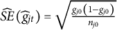 . Where
${n}_{j1}$
 and
${n}_{j0}$
 denote the numbers of examinees classified as masters and non-masters of item
$j$
 at time
$t$
 , respectively. A Laplace correction (additive smoothing; Demidenko, Reference Demidenko2025) was applied by adding 1 to the numerator and 2 to the denominator to ensure stable variance estimation under small sample sizes and to improve numerical stability when parameter estimates approach the boundaries of 0 or 1.
For multivariate monitoring, the univariate residuals are combined into a standardized residual vector. Let
${\widehat{\boldsymbol{\xi}}}_t={\left[{\widehat{s}}_{jt},{\widehat{g}}_{jt}\right]}^T$
 denote the current parameter estimates and
${\boldsymbol{\xi}}_0={\left[{s}_{j0},{g}_{j0}\right]}^T$
 the baseline values. The standardized residual vector is

where
${\boldsymbol{\Sigma}}_{\boldsymbol{0}}= Var\left({\widehat{\boldsymbol{\xi}}}_t-{\boldsymbol{\xi}}_0\right)$
 is the asymptotic covariance matrix evaluated under the IC condition. With the consistent estimators from CMLE (Chen et al., Reference Chen, Xin, Wang and Chang2012),
${\ \widehat{s}}_{jt}$
 is estimated exclusively from the subgroup of examinees who have mastered all required attributes, while
${\widehat{g}}_{jt}$
 is estimated from those who have not. This group-wise separation renders the log-likelihood function separable with respect to
${s}_j$
 and
${g}_j$
 , leading to a diagonal Fisher Information matrix and thus a diagonal
${\boldsymbol{\Sigma}}_{\boldsymbol{0}}$
 . Consequently,
${\boldsymbol{\gamma}}_t$
 asymptotically follows a bivariate standard normal distribution under the IC condition:
${\boldsymbol{\gamma}}_{t}\!\!\sim\!\!{N}_2\left(\boldsymbol{0},{\mathbf{I}}_{\mathbf{2}}\right)$
 , where
${\mathbf{I}}_{\mathbf{2}}$
 denotes the
$2\times 2$
 identity matrix. Under the OC hypothesis,
${\boldsymbol{\gamma}}_{t}\!\!\sim\!\!{N}_2\left({\boldsymbol{\delta}}_t,{\mathbf{I}}_{\mathbf{2}}\right)$
 , where
${\boldsymbol{\delta}}_t={\left[{\delta}_t^{(s)},{\delta}_t^{(g)}\right]}^T$
 .
3.2.2 Benchmark methods: fixed-
$k$
 CUSUM and likelihood ratio test

Two classes of established monitoring methods serve as benchmarks for evaluating the proposed adaptive procedures:
Fixed-
$k$
 CUSUM charts. As described in the previous section, the standard tabular CUSUM accumulates standardized residuals with a constant reference value
$k$
 . This study assumed negative drift in
$s$
 and positive drift in
$g$
 , motivated by the operational hypothesis that, over time, exposure to coaching or item preknowledge may reduce careless errors (lower
$s$
 ) and increase random guessing (higher
$g$
 ). For univariate monitoring, the statistics (denoted
${C}_t^{\left({\mathrm{s}}_f\right)}$
 and
${C}_t^{\left({g}_f\right)}$
 ) were computed using Equations (7) and (8), while the multivariate monitoring statistic (denoted
${MC}^f$
 ) was computed using Equation (3):


To facilitate comparison with the CUSUM control charts and prior research, this study also employed the LRT, which evaluates the goodness of fit between two nested models, targets multiple parameter domains, and supports sequential monitoring within online calibration procedure (Kang, Reference Kang2023). At each monitoring occasion, the null hypothesis is
${H}_0: item\;j\; has\; not\kern0.17em drifted$
 . The test statistic is
${G}^2=-2\mathit{\ln}\left[\frac{L\left({M}_c\right)}{L\left({M}_a\right)}\right]=2\ln \left(L\left({M}_a\right)\right)-2\ln \left(L\left({M}_c\right)\right)$
 . Where
$L\left({M}_c\right)$
 and
$L\left({M}_a\right)$
 represent the likelihoods of the null (
${M}_c$
 ) and alternative (
${M}_a$
 ) model. The
${M}_c$
 uses the original item parameter vector, while
${M}_a$
 incorporates recalibrated item parameters. Under
${H}_0$
 , the test statistic is asymptotically distributed as
${\chi}^2$
 with two degrees of freedom when the slipping and guessing parameters are tested jointly.
3.2.3 Adaptive CUSUM charts
To address the practical limitation of prespecifying the reference value, this study applied the adaptive CUSUM charts from statistical control that detect diverse patterns of drift in time series data (Jiang et al., Reference Jiang, Shu and Apley2008; Yi & Qiu, Reference Yi and Qiu2022). The core modification replaces the fixed reference
$k$
 with a real-time estimation of the drift magnitude,
${\widehat{\delta}}_t$
 , derived from the sequential probability ratio test (SPRT) framework (Haq, Reference Haq2024). Such substitution preserves the local optimality of the SPRT: as
${\widehat{\delta}}_t$
 converges to the true drift magnitude
${\delta}_t$
 , the adaptive CUSUM approaches the optimal chart for that drift size without requiring prior specification of
$k$
 (Jiang et al., Reference Jiang, Shu and Apley2008).
For univariate monitoring, under the IC condition,
${e}_t^{(s)}\!\!\sim\!\!N\left(0,1\right)$
 and
${e}_t^{(g)}\!\!\sim\!\!N\left(0,1\right)$
 . Whereas under the OC condition,
${e}_t^{(s)}\!\!\sim\!\!N\left({\delta}_t^{(s)},1\right)$
 and
${e}_t^{(g)}\!\!\sim\!\!N\left({\delta}_t^{(g)},1\right)$
 . The corresponding log-likelihood ratio (LLR) for
${e}_t^{(s)}$
 comparing the OC and IC hypotheses is given by the following expression, and the derivation for
${e}_t^{(g)}$
 is analogous:

The univariate adaptive CUSUM charts are updated sequentially by accumulating these LLRs with a reflecting boundary at zero:


The recursive form of the multivariate adaptive CUSUM statistic (
$M{C}_t$
 ) under the DINA model is then defined as follows:

3.2.4 Drift magnitude estimation
The adaptive CUSUM framework requires a real-time estimate of the drift magnitude
${\widehat{\delta}}_t$
 , which serves as a dynamic weight that adaptively optimizes chart sensitivity to the detected change. Two methods are used to update this estimate as each new batch of examinee data arrives.
-
(1) Exponentially Weighted Least Square Regression (EWLS):
Following Yi and Qiu (Reference Yi and Qiu2022), the parameter change is modeled as a linear function of time to capture nonstationary trends. For a scalar residual sequence, the
${\widehat{\delta}}_t$
 at time
$t$
 is estimated by solving a weighted least squares problem with exponential decay weights. For example,
${\widehat{\delta}}_t^{(s)}$
 for the slipping parameter is estimated by solving
${\mathit{\min}}_{\alpha, \beta \in R}{\sum}_{n=1}^t{\left({e}_n^{(s)}-{\alpha}_s-{\beta}_sn\right)}^2{\left(1-\lambda \right)}^{t-n}$
 . The decay parameter
$\lambda \in \left[0,1\right]$
 controls the trade-off between sensitivity to recent changes (larger
$\lambda$
 ) and stability based on longer historical trends (smaller
$\lambda$
 ; Han & Kang, Reference Han and Kang2023). The real-time drift estimate is
${\widehat{\delta}}_t^{(s)}={\widehat{\alpha}}_s+{\widehat{\beta}}_st$
 , where the intercept
${\widehat{\alpha}}_s$
 represents the baseline shift level, and the slope
${\widehat{\beta}}_s$
 captures the rate of drift. The real-time drift estimate for the guessing parameter is obtained analogously.
For the multivariate extension, the bivariate drift vector is modeled as
${\boldsymbol{\delta}}_t=\boldsymbol{\alpha} +\boldsymbol{\beta} t$
 , and the weighted sum of squared distances for
${\boldsymbol{\gamma}}_t$
 is minimized as follows:
${\mathit{\min}}_{\boldsymbol{\alpha}, \boldsymbol{\beta} \in {R}^2}{\sum}_{n=1}^t{\left\Vert {\boldsymbol{\gamma}}_n-\boldsymbol{\alpha} -\boldsymbol{\beta} n\right\Vert}^2{\left(1-\lambda \right)}^{t-n}$
 . The real-time drift vector estimate is
${\widehat{\boldsymbol{\delta}}}_t=\widehat{\boldsymbol{\alpha}}+\widehat{\boldsymbol{\beta}}t$
 , where
$\widehat{\boldsymbol{\alpha}}={\left[{\widehat{\alpha}}_s,{\widehat{\alpha}}_g\right]}^T$
 ,
$\widehat{\boldsymbol{\beta}}={\left[{\widehat{\beta}}_s,{\widehat{\beta}}_g\right]}^T$
 .
During the initial stages of monitoring, only a few time points are available for regression, so the weighted design matrix can become nearly singular, producing unstable estimates of regression coefficients. Thus, ridge regression (Hoerl & Kennard, Reference Hoerl and Kennard1970) with a small regularization parameter (1e-4) is applied, ensuring numerical invertibility without substantially biasing estimates once sufficient data accumulates. Together with the Laplace correction and the reflecting boundary at zero in the CUSUM accumulation, it forms one of three safeguards against small-sample instability in early-batch CD-CAT monitoring.
-
(2) Exponentially Weighted Moving Average (EWMA):
As a computationally efficient alternative, the drift magnitude for slipping parameter can be estimated using a ratio of exponentially weighted sums:
${\widehat{\delta}}_t^{(s)}={\sum}_{n=1}^t\frac{e_n^{(s)}{\left(1-\lambda \right)}^{t-n}}{\sum_{n=1}^t{\left(1-\lambda \right)}^{t-n}}$
 . Similar equations are used for
${e}_n^{(g)}$
 and
${\boldsymbol{\gamma}}_t$
 as well. The EWMA estimator utilizes a normalized weighted sum to ensure that the estimator
${\widehat{\delta}}_t$
 remains an unbiased estimate of the current shift magnitude even during the initial stages (Jiang et al., Reference Jiang, Shu and Apley2008; Lucas & Saccucci, Reference Lucas and Saccucci1990). Moreover, because the standardized residuals are asymptotically standard normal under CMLE (Chen et al., Reference Chen, Xin, Wang and Chang2012), the estimator
${\widehat{\delta}}_t$
 is consistent under stationarity, with
${\widehat{\delta}}_t\to {\delta}_t$
 as the per-item sample size increases.
3.3 Online calibration and monitoring procedure
Figure 1 illustrates the real-time IPD monitoring procedure integrated with online calibration. The procedure assumes a CD-CAT item bank of
$M$
 pre-calibrated items, in which IPD may occur over repeated test administrations due to item leakage or exposure (Kang, Reference Kang2023). During test administration, initial item selection follows an attribute-targeted rule to ensure that each attribute is measured by at least one starting item. Subsequent items are selected using the Posterior-Weighted Kullback–Leibler (PWKL) information criterion, which has been widely adopted and shown to be effective in CD-CAT settings (Cheng, Reference Cheng2009; Huang et al., Reference Huang, Zhang, Morphew, Nissen, Van Dusen and Chang2025). To ensure that sufficient response data accumulate across the entire item bank for stable online calibration and monitoring (Kang, Reference Kang2023), the Maximum Priority Index (MPI) method is applied to control item exposure (Cheng & Chang, Reference Cheng and Chang2009).
Procedure for online calibration and real-time IPD monitoring.

Figure 1 Long description
A process diagram of how item parameter drift (IPD) is monitored during CD-CAT. Examinees take repeated administrations from a pre-calibrated item bank, with item selection using an attribute-targeted start, the PWKL criterion, and MPI exposure control. Responses accumulate per item; once an item reaches an admissible sample size, its parameters are recalibrated in sequential batches and converted to standardized residuals that are monitored with a CUSUM statistic. When the CUSUM exceeds the control limit h, the item is flagged as drifted and sent for review, then either discarded or revised and returned to the bank; unflagged items remain in operational use.
Specifically, let
$r=L/M$
 denote the target maximum exposure rate used to promote uniform item usage. For item
$j$
 , administered to
${n}_j$
 of
$N$
 examinees, the exposure constraint is
${f}_{exp}=\max \left({10}^{-5},\frac{r-\left({n}_j/N\right)}{r}\right)$
 , where the
${10}^{-5}$
 is included to maintain numerical stability and prevent the index from becoming zero or negative. An item with a current exposure rate
${n}_j/N$
 below
$r$
 receives a higher
${f}_{exp}$
 , whereas overexposed items are deprioritized. The final priority index for item selection is
$P{I}_j= PWK{L}_j\times {f}_{exp}$
 , and the item with the highest
$P{I}_j$
 is selected. Although PWKL and MPI may induce dependence among item exposure patterns, item selection uses only information available before each response, so the conditional DINA response model remains unchanged. Any effects on subgroup sizes are reflected in the item-specific standard errors. Throughout these repeated administrations, responses are accumulated in item-specific sequential batches to enable efficient and systematic intermittent monitoring. Once an item reaches the admissible sample size, its parameters are recalibrated using all cumulative responses available up to time
$t$
 . This process generates a time series of parameter estimates for item
$j$
 ,
$\left({\widehat{s}}_{j1},{\widehat{g}}_{j1}\right),\dots, \left({\widehat{s}}_{jt},{\widehat{g}}_{jt}\right)$
 .
Recalibration is driven by each item’s accumulated response count rather than by the overall examinee stream. For example, with
$N=\mathrm{8,000}$
 , a fixed test length
$L=30$
 , and
$M=120$
 , the target exposure rate is
$r=L/M=.25$
 , and each item is expected to accumulate approximately
$N\times r=\mathrm{2,000}$
 responses over the testing window. It is first recalibrated after 500 responses and again after each additional batch of 50 responses, yielding approximately (
$\mathrm{2,000}-500)/50=30$
 subsequent recalibration points per item under these conditions. In terms of the examinee stream, the 500-response threshold is expected to be reached after about
$500/r=\mathrm{2,000}$
 examinees. However, this correspondence between per-item response counts and the examinee stream depends on the near-uniform exposure promoted by MPI. In operational CAT, realized exposure rates vary across items, so the timing and number of recalibration points are item-specific.
At each recalibration stage, adaptive CUSUM control charts are applied to detect parameter drift. Specifically, the current parameter estimates are statistically tested against their baseline. An item is flagged as drifted immediately when its CUSUM statistic exceeds the control limit
$h$
 . Following further review, item bank managers may discard the flagged item or revise it by updating its parameters or content, after which the revised item can be reintroduced into the item bank for continued use. Through this procedure, the system supports real-time detection of IPD while maintaining the efficiency of CAT operations.
4 Simulation studies
Assuming that item drift occurs due to item leakage, parameter drift was introduced when the item was assigned to the 1001st examinee, reflecting a realistic scenario in which items remain stable during an initial IC period before drift onset (Kang, Reference Kang2023). To address the research objectives outlined in the Introduction, two simulation studies were designed with complementary evaluation goals. Study 1 conducted a systematic comparison of all detection methods under varying drift conditions, with the goal of simultaneously examining the relative merit of the adaptive approach (Objective 1) and the viability of the overall framework (Objective 2). Study 2 assessed the robustness of the adaptive CUSUM charts under varying operational parameters, thereby strengthening the generalizability of the methodological recommendations derived from Study 1.
4.1 Examinee and item bank generation
Both simulation studies shared a common data generation framework. The number of attributes
$K$
 was set to 4 in Study 1 and varied across
$K=2,4$
 , and 6 in Study 2. Taking
$K=4$
 as an example, there are
${2}^K=16$
 possible attribute mastery profiles. To mirror realistic educational populations, the marginal proportions of examinees mastering 0, 1, 2, 3, and 4 attributes were set to approximately 5%, 25%, 40%, 25%, and 5%, respectively (Huang et al., Reference Huang, Zhang, Morphew, Nissen, Van Dusen and Chang2025; Lin & Chang, Reference Lin and Chang2019). Within each mastery level, profiles with the same number of mastered attributes were assigned equal probabilities. For instance, among examinees who mastered one attribute, the four single-attribute patterns were each assigned a probability of .25/4 = .0625.
The pre-calibrated item pool contained
$M=120$
 items. A
$120\times K$
 Q-matrix was constructed to represent varying cognitive complexity. For
$K=4$
 , the item pool included 20 single-attribute items, 60 two-attribute items, and 40 three-attribute items. Item order was randomized to prevent ordering effects. Under the DINA model, slipping and guessing parameters were generated from a uniform distribution
$U\left(.05,.25\right)$
 , consistent with ideal parameter ranges established in previous studies (Chen et al., Reference Chen, Xin, Wang and Chang2012; Huang et al., Reference Huang, Zhang, Morphew, Nissen, Van Dusen and Chang2025; Yu & Cheng, Reference Yu and Cheng2024). Of the
$M=120$
 items,
$D=12$
 items (10%) were designated as drift items, and previous studies suggest that this proportion has little effect on parameter recovery and attribute estimation under comparable conditions (Cooperman et al., Reference Cooperman, Tai, DeWeese and Weiss2025; Wells et al., Reference Wells, Subkoviak and Serlin2002). These items were evenly allocated across three drift types:
$s$
 -drift,
$g$
 -drift, and
$s$
 g-drift conditions. The remaining
$M-D=108$
 items served as non-drift items. To generate IPD while avoiding non-positive parameter values after drift, drifted items were selectively perturbed. For example, only items with baseline slipping parameters exceeding .15 were subjected to a negative
$s$
 -drift of magnitude .15.
For
$K=2$
 and 6, the same procedure was used. Mastery-level probabilities followed a binomial distribution, Binomial(
$K$
 , .5), producing a symmetric pattern in which extreme mastery levels were rare and intermediate levels were most common. Profiles within each mastery level were assigned equal probabilities. The Q-matrix was constructed with items ranging from single-attribute to (
$K$
 –1)-attribute complexity, with the number of items at each level following a comparable symmetric distribution to ensure balanced attribute coverage.
Each examinee was administered a unique
$30$
 -item test (Kang, Reference Kang2023). Item responses were simulated from a Bernoulli distribution based on the DINA model probabilities. Items were adaptively selected using the PWKL information criterion with the MPI exposure control, targeting an item exposure rate of
$r=L/M=$
 .25. Examinees’ attribute profiles were estimated using the expected a posteriori (EAP) method under a uniform prior over all possible latent attribute classes.
4.2 Design factors
The simulation design manipulates several factors that are expected to influence IPD detection performance. The rationale for each factor is summarized below.
IPD size represents the magnitude of parameter changes for drifted items. Prior research has shown that larger IPD sizes significantly impair parameter estimation accuracy (Cappaert et al., Reference Cappaert, Wen and Chang2018; Kürşad et al., Reference Kürşad, Çokluk-bökeoglu and Çıkrıkçı2022). While some IRT-based studies used fixed magnitudes ranging from .25 to .5 (Guo et al., Reference Guo, Zheng and Chang2015; Kang, Reference Kang2023; Wells et al., Reference Wells, Subkoviak and Serlin2002), these values may be inappropriate for the DINA model, in which slipping and guessing parameters are typically generated from the uniform distribution
$U\left(.05,.25\right)$
 . Building on this, the present study proposes a new set of IPD sizes (.05, .10, and .15) tailored to the characteristics of the DINA model (Chen et al., Reference Chen, Xin, Wang and Chang2012; Huang et al., Reference Huang, Zhang, Morphew, Nissen, Van Dusen and Chang2025; Yu & Cheng, Reference Yu and Cheng2024).
Drift type captures which parameter is affected. Wells et al. (Reference Wells, Subkoviak and Serlin2002) explored a-drift, b-drift, and ab-drift under the 2PL model. Although they found that the parameter recovery was similar across drift types, this factor showed significant interactions with test length and sample size. Cooperman et al. (Reference Cooperman, Tai, DeWeese and Weiss2025) also highlighted that difficulty parameter drift had the most substantial impact on detecting meaningful psychometric changes. To extend this line of inquiry to the DINA model, the present study considers three IPD types: slipping drift (
$s$
 -drift), guessing drift (
$g$
 -drift), and simultaneous drift in both parameters (
$sg$
 -drift).
Drift pattern characterizes the temporal trajectory of parameter change, a critical factor that remains largely unexplored in the existing IPD literature, as traditional non-adaptive monitoring methods are typically designed for abrupt shifts (Kang, Reference Kang2023). However, in operational testing, item parameters may degrade according to different temporal dynamics. For example, a sudden security breach might cause a step drift, whereas item leakage that spreads progressively through social networks may manifest as a gradual drift. Conversely, a shift in instructional focus might lead to a decelerating drift, in which the parameter change is rapid initially but eventually stabilizes. The current study incorporates these three distinct patterns to evaluate whether the IPD monitoring methods can track different real-world scenarios.
Sequential batch size determines how frequently item parameters are re-estimated and monitored. Although the existing literature indicates that test length contributes minimally to recalibrated item-parameter estimation (Huang et al., Reference Huang, Zhang, Morphew, Nissen, Van Dusen and Chang2025; Yu & Cheng, Reference Yu and Cheng2024), increasing sample size generally enhances estimation accuracy (Chen et al., Reference Chen, Xin, Wang and Chang2012; Kürşad et al., Reference Kürşad, Çokluk-bökeoglu and Çıkrıkçı2022; Tan et al., Reference Tan, Wang, Luo, Cai and Tu2024; Wells et al., Reference Wells, Subkoviak and Serlin2002; Yu & Cheng, Reference Yu and Cheng2024). Building on this established knowledge, the current study emphasizes the role of sequential batch size, which affects both the number of examinees available for incremental parameter updates and the length of the monitored parameter-estimate time series
$\left({\widehat{s}}_{jt},{\widehat{g}}_{jt}\right)$
 , making this factor particularly important for systematic investigation.
Decay parameter (
$\lambda$
 ) controls the weighting of recent versus historical observations in the adaptive CUSUM charts. Han and Kang (Reference Han and Kang2023) indicated that
$\lambda$
 values for EWMA-based CUSUM procedures in the range [.03, .27] yielded optimal detection power for all procedures. As
$\lambda$
 increased beyond this range, detection became faster but at the cost of reduced power. This reflects an inherent trade-off between detection power and signaling delay governed by
$\lambda$
 . Accordingly, in the present study, multiple
$\lambda$
 values (.2, .5, and .8) were considered to span low, moderate, and high levels, reflecting different trade-offs between power and signaling speed.
Number of attributes (
$K$
 ) determines the complexity of the diagnostic model and the attribute profile space, making it a fundamental design parameter in CDMs (Hou et al., Reference Hou, la Torre and Nandakumar2014; Huang et al., Reference Huang, Zhang, Morphew, Nissen, Van Dusen and Chang2025). Previous simulation studies in the CDM literature have employed a fixed
$K$
 , often in the range of 4–6, to model typical diagnostic scenarios (e.g., Chen et al., Reference Chen, Xin, Wang and Chang2012; Nájera et al., Reference Nájera, Abad and Sorrel2021). To systematically evaluate the robustness of the proposed method, this study considers
$K=2,4$
 , and
$6$
 , ranging from simple to relatively high-dimensional diagnostic scenarios.
4.3 Study 1: Core comparison of detection methods under varied drift conditions
Study 1 conducted a systematic comparison of all detection methods under varied drift conditions. Four factors were manipulated: (1) IPD Detection Method (LRT, adaptive CUSUM based on EWLS:
${C}^{EWLS}$
 and
$M{C}^{EWLS}$
 , or EWMA:
${C}^{EWMA}$
 and
${MC}^{EWMA}$
 , fundamental CUSUMs with fixed
$k=1$
 :
${C}^{f1}$
 and
${MC}^{f1}$
 , or fixed
$k=2.5$
 :
${C}^{f2.5}$
 and
$M{C}^{f2.5}$
 ). (2) IPD Size (.05, .10, .15). (3) Drift Type (
$s$
 -drift,
$g$
 -drift,
$s$
 g-drift). (4) Drift Pattern (abrupt, gradual, decelerating). Other parameters are fixed at typical values: sequential batch size = 150, decay parameter
$\lambda =.5$
 , and the number of attributes
$K=4$
 . Each condition had a total of 100 replications to ensure reliability.
In classical CUSUM theory, the optimal reference value can be set as
$k=\delta /2$
 (Lee et al., Reference Lee, Lewis, von Davier, Yan, von Davier and Lewis2014; Lee & Lewis, Reference Lee and Lewis2021), where the
$\delta$
 depends on both the raw IPD size and the standard error of the parameter estimate, which may differ across parameters. Under the conditions of this study,
$k=1$
 tends to underestimate the optimal reference value across most drift conditions, while
$k=2.5$
 falls within a plausible optimal range for both slipping and guessing parameters. By including both values, the simulation examined how detection performance varies when the fixed value of
$k$
 either underestimates or reasonably approximates the unknown drift magnitude.
After IPD onset, the item parameters of drift items evolved according to one of three drift patterns. Take the slipping parameter as an example, let
${s}_{j0}$
 be the initial pre-calibrated baseline for item
$j$
 , and let
${s}_j^{\ast }$
 denote the final, fully drifted target value. We define
${t}^{\ast }=\frac{n_j-1000}{N-1000}\in \left[0,1\right]$
 as the normalized time elapsed since drift onset, where
${n}_j$
 indexes the examinee sequence. Under abrupt drift,
${s}_{j0}^{\ast }={s}_j^{\ast }$
 for all
${t}^{\ast }>0$
 , where
${s}_{j0}^{\ast }$
 is the true post-drift parameter against which the re-estimated
${\widehat{s}}_{jt}$
 is compared. Under gradual drift, item parameters change linearly from baseline values to the fully drifted values across the remaining examinees:
${s}_{j0}^{\ast }={s}_{j0}+{t}^{\ast}\left({s}_j^{\ast }-{s}_{j0}\right)$
 . Under decelerating drift, item parameters change rapidly shortly after onset and then approach the fully drifted values more slowly, following a concave quadratic trajectory:
${s}_{j0}^{\ast }={s}_{j0}+\left[1-{\left(1-{t}^{\ast}\right)}^2\right]\times \left({s}_j^{\ast }-{s}_{j0}\right)$
 . For non-drift items,
${s}_{j0}^{\ast }={s}_{j0}$
 , and the guessing parameter follows analogously.
Control limit values (
$h$
 ) for each CUSUM method were obtained empirically through a Monte Carlo simulation under the null condition (no IPD). To maintain the overall Type I error rate (family-wise error rate, FWER) at
$\alpha =.05$
 , the maximum value of each statistic was recorded within each of the 100 replications. The control limit
$h$
 was then set as the (1-
$\alpha$
 ) quantile of these maxima. Because the null simulations reproduce the full CD-CAT design, including PWKL selection, MPI exposure control, profile estimation, and sequential recalibration, the resulting control limits incorporate the cross-item and temporal dependence induced by the design rather than relying on an independence assumption. These design-specific limits should be recalibrated when substantially different item-selection or exposure-control procedures are used.
4.4 Study 2: Sensitivity analysis on operational factors
Building on Study 1, Study 2 evaluated the robustness and practical applicability of the proposed adaptive CUSUM charts (
${C}^{EWLS}$
 ,
$M{C}^{EWLS}$
 ,
${C}^{EWMA}$
 and
${MC}^{EWMA}$
 ) under varying operational conditions. Three operational factors were varied: (1) Sequential Batch Size (50, 150, 300). (2) Number of Attributes (
$K=2,4,$
 6). (3) Decay Parameter (
$\lambda =$
 .2, .5, .8). Other parameters in study 1 were fixed at IPD Size = .10, Drift Pattern = abrupt. Each condition was replicated 100 times.
4.5 Evaluation criteria
The effectiveness of the MPI exposure control in achieving uniform item usage and the accuracy of attribute profile estimation, which was evaluated using the average Attribute Correct Classification Rate (
$\overline{ACCR}=\frac{1}{N}\frac{1}{K}{\sum}_{k=1}^K{\sum}_{i=1}^NI\left({\widehat{\alpha}}_{ik}={\alpha}_{ik}\right)$
 ; Huang et al., Reference Huang, Zhang, Morphew, Nissen, Van Dusen and Chang2025), are reported as verification checks for the CD-CAT simulation environment.
$I\left[.\right]$
 denotes an indicator function, and
${\alpha}_{ik}$
 and
${\widehat{\alpha}}_{ik}$
 are the true and estimated mastery statuses for attribute
$k$
 of examinee
$i$
 , respectively.
IPD detection performance was evaluated based on three primary criteria:
-
(1) Type I error rate ( $\boldsymbol{\alpha}$
; Guo, Reference Guo2016; Kang, Reference Kang2023) was evaluated in two ways: the per-item Type I error rate (
${\alpha}_{per- item}$
) measures the proportion of non-drift items falsely flagged across replications. Let
$R=100$
denote the total number of replications. The per-item
$\alpha$
was calculated as follows:(13) $$\begin{align}{\alpha}_{per- item}=\frac{\sum \limits_{r=1}^R{\sum}_{i^{\ast}\in non- drift\kern0.17em items}I\left( ite{m}_{i^{\ast }}\; flagged\right)}{R\left(M-D\right)}\end{align}$$


The FWER (
${\alpha}_{FWER}$
 ) measures the proportion of replications in which at least one non-drift item was falsely flagged, consistent with the max-statistic calibration used to determine the control limits:

-
(2) Average detection delay ( $ADD$
) evaluates detection speed. For each drifted item, the run length (
$RL$
) is defined as the number of post-drift monitoring batches that elapse until the first out-of-control signal (Kang, Reference Kang2023; Lee & Lewis, Reference Lee and Lewis2021). The
$ADD$
is the mean
$RL$
across successfully detected drifted items, reflecting how quickly drift is identified after its onset. The
$RL$
clock begins at the first monitoring batch following drift onset (examinee 1001). Given the remaining testing window after drift introduction,
$RL$
is a discrete value with a minimum of 1. The maximum possible
$RL$
values were 6, 11, and 31 for batch sizes of 300, 150, and 50, respectively. Because each item is administered to an expected 25% of examinees, batches of 300, 150, and 50 item responses correspond to approximately 1,200, 600, and 200 examinees, respectively.
$ADD$
is, therefore, reported in both monitoring batches and equivalent examinee counts. -
(3) Detection power represents the sensitivity of the monitoring procedures. Following Kang (Reference Kang2023), power levels are interpreted as excellent ( $\ge .8$
), moderate (
$.6,.8$
), and low (
$<.6$
). To facilitate comparison between univariate and multivariate monitoring schemes, separate power metrics are reported.


For multivariate detection power, five methods were evaluated: LRT,
$M{C}^{EWLS}$
 ,
${MC}^{EWMA}$
 ,
${MC}^{f1}$
 , and
$M{C}^{f2.5}$
 . Power was computed across all drifted items:

For univariate detection power, only the four CUSUM charts (
${C}^{EWLS}$
 ,
${C}^{EWMA}$
 ,
${C}^{f1}$
 ,
${C}^{f2.5}$
 ) were considered, as the LRT does not provide parameter-specific signals. The slipping monitor (
$powe{r}_s$
 ) was evaluated using items with
$s$
 -drift and
$sg$
 -drift, and the guessing monitor (
$powe{r}_g$
 ) is defined analogously:


5 Simulation results
5.1 Study 1 results
This section focuses on the evaluation of real-time IPD detection within the CD-CAT framework and the comparative performance of the detection methods. As a preliminary verification, item exposure tracking confirmed that nearly every item was administered 11 or 12 times, achieving the desired uniformity. Across all conditions, the average
$\overline{ACCR}$
 values across 100 replications exceeded .921 (
$SD\approx .004$
 ), confirming accurate attribute estimation and stable calibration. These results establish a stable and reliable CD-CAT environment for evaluating detection performance. A summary of the Study 1 simulation results is presented in Table A1.
5.1.1 Type I error
The proposed framework demonstrated effective false alarm control using CUSUM-based monitoring. Across all conditions, the CUSUM charts maintained
${\alpha}_{per- item}$
 near zero and kept
${\alpha}_{FWER}$
 close to the nominal .05 level. In contrast, the LRT method showed severely inflated false alarm rates (
${\alpha}_{FWER}=~1;{\alpha}_{per- item}\approx .17$
 ), rendering it impractical for real-time monitoring. This inflation arises from repeated testing: although each individual
${\chi}^2$
 test is correctly sized at
$\alpha =.05$
 , the probability of at least one false alarm accumulates across items and repeated monitoring occasions, driving
${\alpha}_{FWER}$
 toward 1 in moderately long sequences.
To compare CUSUM variants, main-effects ANOVAs on
${\alpha}_{FWER}$
 (excluding the LRT) were conducted. The choice of CUSUM variant significantly influenced only slipping parameter monitoring (
$F\left(3,28\right)=17.77,p<.001,{\eta}_p^2=.656$
 ). Adaptive CUSUMs (
${C}^{EWLS}$
 ,
${C}^{EWMA}$
 ) yielded slightly higher
${\alpha}_{FWER}(\approx .076$
 ) than fixed-
$k$
 CUSUMs (
${C}^{f1}:.021$
 ,
${C}^{f2.5}:.018$
 ), reflecting the cost of self-tuning. However, no significant method differences were observed for guessing (
$F\left(3,28\right)=.194,p=.899,{\eta}_p^2=.020$
 ) or multivariate monitoring (
$F\left(3,28\right)=1.032,p=.394,{\eta}_p^2=.100$
 ).
Drift pattern significantly influenced
${\alpha}_{FWER}$
 for both guessing (
${\eta}_p^2=.528$
 ) and multivariate monitoring (
${\eta}_p^2=.595$
 ). Decelerating drift yielded the lowest mean
${\alpha}_{FWER}$
 (guessing:
$M=.009, SD=.014$
 ; multivariate:
$M=.033, SD=.018$
 ), whereas gradual drift produced the highest (guessing:
$M=.042, SD=.018$
 ; multivariate:
$M=.048, SD=.007$
 ). IPD size affected only multivariate monitoring (
$F\left(2,28\right)=66.764,p<.001,{\eta}_p^2=.827$
 ), showing a nonlinear pattern, with the lowest error at medium IPD-size level (
${\alpha}_{FWER}=.026$
 ).
5.1.2 ADD values
The
$ADD$
 analysis showed that, among successfully detected items, all monitoring methods generally signaled drift before the full sample had accumulated, demonstrating the viability of real-time IPD detection within the CD-CAT framework. For univariate monitoring, shifts in the guessing parameter were generally detected approximately two batches faster than shifts in the slipping parameter. For the slipping parameter, the mean
$ADD$
 values were
$AD{D}_{C^{EWLS}}=9.71$
 batches (
$\approx \mathrm{5,826}$
 examinees),
$AD{D}_{C^{EWMA}}=9.70$
 batches (
$\approx \mathrm{5,820}$
 examinees),
$AD{D}_{C^{f1}}=10.07$
 batches (
$\approx \mathrm{6,042}$
 examinees),
$AD{D}_{C^{f2.5}}=9.48$
 batches (
$\approx \mathrm{5,688}$
 examinees), reflecting the inherently greater estimation difficulty of the slipping parameter under the DINA model.
Multivariate monitoring consistently yielded faster detection than univariate monitoring. Although the LRT showed shorter
$ADD$
 , this advantage was offset by its poor false alarm control. ANOVA results (Table 1) identified that IPD size (
${\eta}_p^2=.858$
 ) and drift pattern (
${\eta}_p^2=.862$
 ) were the dominant factors. As expected, larger IPD sizes significantly reduced detection delay, with mean
$ADD$
 values of 6.07, 7.46, and 9.49 batches for large, medium, and small IPD, respectively, corresponding to approximately 3,642, 4,476, and 5,694 examinees. Abrupt drift was detected after an average of 5.74 batches, corresponding to approximately 3,444 examinees, compared with 9.16 batches, or 5,496 examinees, for gradual drift and 8.11 batches, or 4,866 examinees, for decelerating drift. These results indicate that less abrupt parameter shifts require more observations to reach the statistical threshold for an OC signal.
Main effects ANOVA for multivariate monitoring
$ADD$


Table 1. Long description
Rows are the factors drift pattern, IPD size, method, and residuals; columns are degrees of freedom, sum of squares, mean square, F, and p-value. IPD size and drift pattern are the dominant factors, with partial eta-squared of .858 and .862, respectively.
Note: Df represents the degree of freedom, sum sq. stands for sum of squares, and mean sq. represents mean square.
The choice of detection method was also statistically significant (
${\eta}_p^2=.260$
 ). While
${MC}^{f2.5}$
 achieved the fastest detection (
$ADD$
 = 7.40 batches or 4,440 examinees), the
${MC}^{f1}$
 was the slowest (
$ADD$
 = 8.25 batches or 4,950 examinees), illustrating the inherent risks of relying on fixed reference values. Adaptive CUSUMs (
${MC}^{EWLS}$
 : 7.51 batches or 4,506 examinees,
$M{C}^{EWMA}$
 : 7.52 batches or 4,512 examinees) yielded detection speeds close to that of the better-performing fixed-
$k$
 benchmark (
${MC}^{f2.5}$
 ), without requiring prior specification of
$k$
 . No meaningful interaction effects were observed.
5.1.3 Detection power
The detection power analysis indicated that the proposed framework achieves strong sensitivity under moderate-to-large IPD while revealing important boundary conditions for CD-CAT monitoring. Factorial ANOVAs (Table 2) revealed that drift pattern and IPD size were the dominant factors for all three monitoring schemes, with a significant interaction between these factors, indicating that detection difficulty depends on the specific combination of conditions. Under favorable conditions, detection was excellent: averaging across CUSUM methods, abrupt drift with large IPD (.15) yielded
$powe{r}_s=$
 .979,
$powe{r}_g=$
 1.000, and
$powe{r}_m=$
 .991, whereas abrupt drift with medium IPD (.10) maintained
$powe{r}_s=$
 .865,
$powe{r}_g=$
 .971, and
$powe{r}_m=$
 .906. Under gradual drift with small IPD (.05), detection power approached zero for all monitoring schemes (Figure 2), suggesting a practical sensitivity limit.
Two-way ANOVA for univariate and multivariate monitors detection power

Table 2. Long description
Rows are the factors (method, drift pattern, IPD size, their two-way interactions, and residuals); columns give degrees of freedom, mean square, and F separately for the slipping, guessing, and multivariate power outcomes. Drift pattern and IPD size are the dominant factors across all three monitors.
Note: Df represents the degree of freedom, mean sq. represents mean square, and * indicates p-value less than .05.
Overall detection power under univariate and multivariate monitoring.

Figure 2 Long description
A 3 × 3 matrix of line charts. Columns are the slipping monitor (power_s), guessing monitor (power_g), and multivariate monitoring (power_m); rows are abrupt, decelerating, and gradual drift. In each panel the x-axis is IPD size (.05, .10, .15) and the y-axis is detection power from 0 to 100%. Univariate panels compare four CUSUM charts (C^EWLS, C^EWMA, C^f1, C^f2.5); multivariate panels add the LRT. Detection power rises with IPD size throughout. Under abrupt drift the CUSUM charts outperform the LRT in multivariate monitoring, whereas under decelerating and gradual drift the LRT outperforms the CUSUM charts. The guessing and multivariate monitors reach high power under moderate-to-large drift, while the slipping monitor is consistently lower. Exact values are in Appendix Table I.
For univariate monitoring, the choice of detection method was statistically significant for both
$powe{r}_s$
 and
$powe{r}_g$
 , but no significant interactions were found between the detection method and either drift pattern or IPD size (Table 2), suggesting that the relative effectiveness of the detection algorithms remained stable across conditions. A detailed inspection of Figure 2 showed that for slipping parameter detection, the fixed-
$k$
 CUSUMs achieved higher sensitivity:
${C}^{f2.5}\left(M=.401\right)>{C}^{f1}\left(M=.319\right)>{C}^{EWLS}\left(M=.282\right)\approx {C}^{EWMA}\left(M=.281\right)$
 . For guessing parameter detection, this pattern reversed:
${C}^{f2.5}\left(M=.603\right)\approx {C}^{EWLS}\left(M=.600\right)>{C}^{EWMA}\left(M=.597\right)>{C}^{f1}\left(M=.561\right)$
 . This trade-off may reflect the self-tuning characteristic of the adaptive CUSUMs: the dynamic
${\widehat{\delta}}_t$
 estimator may respond more effectively to the better-estimated guessing parameter while sacrificing some sensitivity to the noisier slipping parameter.
Turning to the multivariate framework, method effects were substantial and interacted with drift pattern and IPD size. As illustrated in Figure 2, the method by drift pattern interaction manifested as a crossover: under abrupt drift, the CUSUM methods (
$powe{r}_m\in$
 [.743, .770]) substantially outperformed the LRT (.551), whereas under gradual drift, the LRT (.884) substantially outperformed all CUSUMs ([.246, .283]). A similar reversal occurred under decelerating drift (LRT: .803 vs. CUSUMs: [.388, .420]). This pattern suggests that the CUSUM procedures were more responsive to abrupt changes, whereas the LRT retained greater sensitivity under gradually evolving drift. Such a distinction is operationally relevant because CDM drift mechanisms, particularly item leakage, may produce relatively abrupt changes in item functioning. Among the four CUSUM variants, the adaptive CUSUMs consistently and slightly exceeded the fixed-
$k$
 variants (e.g., abrupt:
${MC}^{EWLS}(.770)>{MC}^{EWMA}(.768)>{MC}^{f2.5}(.766)>{MC}^{f1}(.743)$
 ).
5.2 Study 2 results
Study 2 evaluated the robustness of the adaptive CUSUM charts under three operational factors: the number of attributes
$K$
 , sequential batch size, and the decay parameter
$\lambda$
 , across both univariate and multivariate monitoring schemes. Across all 27 conditions, EWLS and EWMA exhibited highly similar patterns across all evaluation criteria. Specifically, the absolute differences between the two methods did not exceed .01 in FWER, .05 in detection power, or .17 batches in
$ADD$
 . Given this consistency, we selected EWLS as the representative method in the main text. The corresponding EWLS and EWMA numerical results are provided in Table A2. Furthermore, Figure 3 presents the marginal effects of the three operational factors on FWER, detection power, and
$ADD$
 for the EWLS method.
Marginal effects of each factor on
${\alpha}_{FWER}$
 , power, and
$ADD$
 based on EWLS.

Figure 3. Long description
A 3 × 3 matrix of line charts based on the EWLS method. Rows are family-wise error rate (FWER), detection power, and average detection delay (ADD); columns are number of attributes K (2, 4, 6), batch size (50, 150, 300), and decay parameter λ (.2, .5, .8). Each panel plots three monitors: slipping, guessing, and multivariate. The slipping monitor’s power follows an inverted-U across K (lowest at K=2, highest at K=4, lower at K=6), while the guessing and multivariate monitors stay high. ADD decreases markedly as batch size increases, and varying λ produces negligible differences across all three criteria. Exact values are in Appendix Table II.
5.2.1 Effect of the number of attributes
$\boldsymbol{K}$

As shown in Figure 3 and Table A2, varying
$K$
 produced differential effects across monitoring schemes and evaluation criteria. For Type I error, the slipping monitor achieved the lowest
${\alpha}_{FWER}$
 at
$K=4$
 and the highest at
$K=6$
 , whereas the guessing monitor showed negligible variation across
$K$
 (< .01). In contrast, the multivariate chart exhibited a clear increasing trend, with
${\alpha}_{FWER}$
 rising from .030 at
$K=2$
 to approximately .063–.066 at
$K=4$
 and
$K=6$
 . This pattern indicates that the multivariate chart was conservative when the attribute space was small and moved closer to the nominal level once
$K\ge 4$
 .
$ADD$
 remained stable across
$K$
 , with absolute differences of no more than approximately 1.3 batches for all monitoring schemes. Detection power, however, showed distinct patterns by monitor. The guessing and multivariate monitors remained near the ceiling across all
$K$
 values, indicating strong robustness. However, the slipping monitor exhibited an inverted-U pattern, with power increasing from .14 at
$K=2$
 to .70 at
$K=4$
 , then decreasing to .34 at
$K=6$
 .
5.2.2 Effect of sequential batch size
Varying batch size produced negligible effects on Type I error and detection power. In contrast,
$ADD$
 decreased markedly as batch size increased, but
$ADD$
 alone did not reflect the total number of examinees required for detection. For example, for the slipping monitor,
$ADD$
 decreased from 24.98 batches at batch size = 50 to 9.15 at batch size = 150 and 5.26 at batch size = 300. However, when converted to approximate equivalent examinee counts (
$ADD\times$
 batch size /
$r$
 ), the pattern was reversed: 24.98
$\times$
 50 / .25 = 4,996, 9.15
$\times$
 150 / .25 = 5,490, and 5.26
$\times$
 300 / .25 = 6,312. Thus, although
$ADD$
 in batches decreased, the approximate equivalent number of examinees required for detection increases with batch size. Therefore, when detection delay is expressed in terms of equivalent examinee counts, smaller batch sizes lead to earlier detection, highlighting the importance of interpreting
$ADD$
 in conjunction with batch size.
5.2.3 Effect of decay parameter
$\boldsymbol{\lambda}$

Varying
$\lambda$
 produced negligible differences across all three evaluation criteria, cell-level variation across values of
$\lambda$
 did not exceed .01 in
${\alpha}_{FWER}$
 , .016 in detection power, or .12 batches in
$ADD$
 . This pattern differs from Han and Kang (Reference Han and Kang2023), who reported a systematic trade-off between
$\lambda$
 and power across a wider range. However, this difference is informative rather than contradictory. In the present CD-CAT setting, the post-drift detection window was short (typical
$ADD$
 $\approx$
 3–12 batches). As a result, the recency-versus-history weighting controlled by
$\lambda$
 had limited opportunity to accumulate before detection occurs. Accordingly,
$\lambda$
 may become consequential in longer monitoring sequences where memory effects accumulate, but it exerted minimal influence in short-window settings. This negligible effect supports the use of
$\lambda =.5$
 as the representative setting in Study 1.
6 Real data example
The empirical analysis serves as an illustrative application of the proposed real-time IPD detection framework to a real-world educational dataset, demonstrating its operational behavior and interpretability under realistic data conditions.
6.1 Data source
Real response data were collected from pre- and post-tests administered through the Mechanics Cognitive Diagnostic (MCD) program, hosted on the Learning About STEM Student Outcomes (LASSO) platform (https://lassoeducation.org; Van Dusen, Reference Van Dusen2018; Le et al., Reference Le, Nissen, Tang, Zhang, Mehrabi, Morphew, Chang and Van Dusen2025). The pre-test, conducted at the beginning of the semester, included 24,266 examinees, while the post-test, administered 15 weeks later (after the semester), included 19,379 examinees. The instrument was the Force Concept Inventory (FCI), which consists of 30 items measuring two core attributes: vector application and conceptual relationships (Le et al., Reference Le, Nissen, Tang, Zhang, Mehrabi, Morphew, Chang and Van Dusen2025).
6.2 Initial calibration
Student attribute profiles were estimated using the EAP method. Initial item parameters under the DINA model were calibrated separately for the pre- and post-tests using the GDINA package in R (Ma & de la Torre, Reference Ma and de la Torre2020). Within the monitoring pipeline, item parameters were re-estimated using the same CMLE (Chen et al., Reference Chen, Xin, Wang and Chang2012) procedure with Laplace smoothing that was applied in the simulation study. This design promotes consistency between baseline and sequential estimates and guarantees convergence to the same parameter values as sample size increases. Notably, slipping parameters decreased and guessing parameters increased over time, consistent with the simulated drift scenarios.
To construct a defensible drift reference set for evaluating drift detection, a two-criterion labeling rule was applied. An item was labeled as drifted only if (a) the change (
$\Delta$
 ) in at least one item parameter exceeded
$\mid .05\mid$
 , and (b) the MH test (Holland & Thayer, Reference Holland, Thayer, Wainer and Braun1988) was significant at the
$\alpha =$
 .05 level with MH-D-DIF statistic of at least 1.2, following ETS guidelines (Zwick, Reference Zwick2012). Under this item-level rule, which aligns directly with the multivariate monitoring scheme, 16 of 30 items (53.3%) were labeled as drifted. Results from univariate monitoring were interpreted based on parameter-specific shifts in slipping and guessing. Because the true IPD status of the empirical items was not directly observed, this two-criterion rule served as an operational reference rather than definitive ground truth.
6.3 Item monitoring design
All methods (
$LRT,{C}^{EWLS},{C}^{EWMA},{C}^{f1},{C}^{f2.5},{MC}^{EWLS},{MC}^{EWMA},{MC}^{f1}$
 , and
${MC}^{f2.5}$
 ) were applied to monitor IPD periodically across the 30 FCI items. Pre-test parameter estimates served as IC baselines (
${s}_{j0},{g}_{j0}$
 ). Because the dataset consists of two cross-sectional administrations, real-time monitoring was approximated by treating the post-test responses as an “as-if” continuous sequence.
To assess robustness to the ordering of examinees, the procedure was repeated under 10 independent random orderings of the post-test sample. Each replication was generated by applying a distinct random seed to permute the examinees, after which the permuted sequence was divided into batches of 300 and processed sequentially, yielding approximately 63 monitoring time points per item. Evaluation criteria (
${\alpha}_{per- item}$
 , power, and detection time) were reported as means across replications.
Control limits (
$h$
 values) were derived from the pre-test data, which served as the IC baseline. Each limit was set to the maximum IC statistic across all 30 items and monitoring points since only a single pre-test sample is available. The resulting multivariate limits were
$h=6592.39$
 (
${MC}^{EWLS}$
 ), 6583.09 (
${MC}^{EWMA}$
 ), 819.81 (
${MC}^{f1}$
 ), and 705.62 (
${MC}^{f2.5}$
 ). The univariate slipping limits ranged from 49.70 (
${C}^{f2.5}$
 ) to 2687.59 (
${C}^{EWLS}$
 ), and the guessing limits from 470.90 (
${C}^{f2.5}$
 ) to 3904.80 (
${C}^{EWLS}$
 ) across the four charts. The larger empirical limits reflect the scale and dependence structure of the statistics under this calibration design, including the larger number of monitoring occasions and the use of cumulative parameter estimates. Other design parameters (e.g.,
$\lambda =.5$
 for the adaptive CUSUM charts) remained consistent with those used in the simulation study.
6.4 Empirical item monitoring results
The two-criterion labeling rule provides an item-level operational reference, making multivariate monitoring the primary basis for evaluating detection accuracy under the adopted rule. The univariate CUSUMs test parameter-specific drift and are reported for completeness. The standard deviations of each evaluation criterion across the 10 random orderings were small in absolute magnitude across all methods (
$S{D}_{\alpha_{per- item}}\le .041$
 ;
$S{D}_{power}\le .026$
 ;
$S{D}_{detect\kern0.17em time}\le 1.1$
 batches) and were even smaller for multivariate monitoring. This stability indicates that the reported means are relatively insensitive to the ordering of examinees in the posttest sequence. The per-item detection results are presented in Table A3.
6.4.1 Multivariate monitoring for real data
As shown in Table A3, across the 10 random orderings, the LRT flagged every non-drift item in each replication, consistent with the simulation results. This indicates poor control of Type I error, although the LRT achieved the fastest average detection time. This inflation arises because the LRT applies an item-level critical value at each test, causing the FWER to accumulate across items and batches.
In contrast, all multivariate adaptive and fixed-
$k$
 CUSUM charts maintained strong control of per-item false alarms. Only one non-drift item (Item 20) was incorrectly flagged by the proposed adaptive CUSUM charts, and this flag occurred at the very end of the monitoring sequence (around batch 62 out of 63), suggesting that it resulted from a late-stage accumulation effect rather than an early and operationally consequential false alarm. Furthermore, all four multivariate CUSUM charts successfully identified every drifted item in each replication (
$powe{r}_m=1.000$
 ). Among the detected items, the multivariate adaptive CUSUMs achieved faster detection, with an overall average detection time of approximately 28.571 batches. The fixed-
$k$
 CUSUMs were slower, with mean detection times of 36.488 (
${MC}^{f1}$
 ) and 34.794 (
${MC}^{f2.5}$
 ) batches.
6.4.2 Univariate monitoring for real data
Overall, the univariate and multivariate monitoring schemes showed strong agreement in their flagging decisions. Within the adaptive framework, the EWLS and EWMA estimators produced nearly identical results, with complete agreement in detection decisions and mean detection times across items.
A clear asymmetry emerged between slipping and guessing parameter monitoring. For slipping parameters, the adaptive CUSUMs exhibited a more conservative detection pattern than the fixed-
$k$
 CUSUMs, effectively filtering out minor fluctuations. For example, non-drifted items with very small slipping changes (
$\mid {\Delta }_s\mid \le$
 .03), such as Items 6 and 7, were incorrectly flagged by the
${C}^{f1}$
 and
${C}^{f2.5}$
 but not by the
${C}^{EWLS}$
 and
${C}^{EWMA}$
 . Even for moderate shifts, such as that of Item 2 (
${\Delta }_s=$
 −.11), the adaptive methods required substantially more evidence to signal drift (more than 40 batches on average), compared with fewer than 20 batches for the fixed-
$k$
 charts.
In contrast, guessing parameter monitoring showed a clear advantage for the adaptive methods. For items with meaningful
$g$
 -drift (
$\left|{\Delta }_g\right|>$
 .05),
${C}^{EWLS}$
 and
${C}^{EWMA}$
 consistently detected drift faster than the fixed-
$k$
 charts. For example, for Items 4 and 17, the adaptive CUSUMs signaled drift at 12.4 and 17.4 batches, respectively, reducing detection time by roughly 20%–35% compared with
${C}^{f1}$
 and
${C}^{f2.5}$
 .
7 Conclusion and discussion
7.1 Overall summary and key findings
Over time, items within an item bank may undergo systematic parameter changes that compromise score interpretation and threaten testing fairness. This study addresses this issue by developing the first real-time, item-level IPD detection framework for CD-CAT. Two simulation studies and an empirical application to the LASSO MCD dataset jointly support the study objectives. First, the transition from post hoc to real-time detection, previously established for IRT models (Guo et al., Reference Guo, Robin and Dorans2017; Kang, Reference Kang2023), is extended to CDM-based assessments. Second, the need to prespecify the CUSUM reference value
$k$
 (Lee & Lewis, Reference Lee and Lewis2021; Veerkamp & Glas, Reference Veerkamp and Glas2000) is eliminated through a self-tuning estimator embedded within the monitoring statistic.
Across the simulation and empirical analyses, the proposed framework successfully identifies drifted items during test administration. In the empirical study, the mean detection time was substantially shorter than the interval between the pre- and post-tests (Table A3). This finding indicates that real-world contamination can exceed the capacity of passive correction methods to address drift in a timely manner, thereby highlighting the operational necessity of real-time monitoring.
Regarding detection methods, the LRT (Kang, Reference Kang2023) achieved the shortest ADD and showed advantages under gradual and decelerating drift. However, its inflated Type I error rate limits its practical use, as it produces excessive false alarms. In contrast, all CUSUM variants maintained
${\alpha}_{per- item}$
 near zero and
${\alpha}_{FWER}$
 relatively close to the nominal .05 level, supporting more reliable operation. This difference reflects a fundamental mechanism: CUSUM accumulates directional evidence and is effective for sustained shifts, whereas the LRT evaluates global model fit at each batch and is more sensitive to distributed changes.
When comparing adaptive and fixed-
$k$
 CUSUM charts (Kang, Reference Kang2023; Lee & Lewis, Reference Lee and Lewis2021), the results show that adaptive methods provide modest advantages under abrupt drift, which is a particularly relevant scenario for CD-CAT item security, since item leakage can immediately change how items function for specific mastery patterns. This advantage becomes more pronounced under multivariate monitoring. Within the adaptive family, EWLS and EWMA produced nearly identical performance across
${\alpha}_{FWER}$
 , detection power, and ADD, indicating that the two estimators are largely interchangeable under the examined conditions.
The key distinction between adaptive and fixed-
$k$
 CUSUM charts lies in their response to estimation variability. For parameters with higher variability (e.g., slipping), an adaptive CUSUM may occasionally overestimate
${\widehat{\delta}}_t$
 due to noisy residuals. In contrast, fixed-
$k$
 CUSUM charts remain stable because their reference value is constant and does not respond to noise. As a result, adaptive methods tend to be more conservative and require stronger evidence before signaling true drift, whereas fixed-
$k$
 charts may detect changes more quickly when the reference value is optimally chosen. Importantly, this limitation is mitigated under multivariate monitoring, where information from the more stable parameter (e.g., guessing) reduces the influence of noise associated with the other parameter (e.g., slipping). Consequently, the advantages of adaptive CUSUM methods become most evident in multivariate settings, which are also particularly relevant for operational item-bank monitoring.
Additional findings further clarify the role of design factors. Larger IPD magnitudes consistently reduced ADD and increased detection power, which aligns with prior results (Kang, Reference Kang2023). Their effect on Type I error, by contrast, was non-monotonic and confined to multivariate monitoring, where the FWER was lowest at the medium IPD level while remaining near the nominal .05 level. The role of sequential batch size, a previously underexplored factor, was also clarified. The results reveal that smaller batches can detect IPD faster because they permit more frequent parameter re-estimation and monitoring cycles, thereby requiring fewer total examinees for drift detection. The decay parameter
$\lambda$
 had a negligible influence within the examined range, with minimal variation across all evaluation criteria.
The effect of the number of attributes (
$K$
 ) was concentrated in slipping detection and followed a non-monotonic pattern. As
$K$
 increases and higher-complexity items enter the Q-matrix, the subgroup of examinees who master all required attributes shrinks sharply, reducing the effective sample size for slipping estimation and helping to explain the decline in power from
$K=4$
 to
$K=6$
 . This explanation does not extend to
$K=2$
 , where all items are single-attribute, the master and non-master subgroups are approximately balanced in this study, and attribute classification is most accurate among the examined conditions. The lower slipping power at
$K=2$
 may therefore reflect other features of the testing configuration, such as the restricted Q-matrix structure or its interaction with adaptive item selection, and warrants further investigation.
7.2 Operational guidance for item bank maintenance
Grounded in the findings above, three distinct performance profiles emerge. The LRT is sensitive yet aggressive, prioritizing speed at the cost of a high false alarm rate. The fixed-
$k$
 CUSUM charts are specific yet rigid, effectively controlling false alarms but relying on a prespecified reference value, with performance highly sensitive to this choice. The adaptive CUSUM charts are conservative yet flexible, effectively adapting to unknown drift magnitudes but requiring more time to accumulate sufficient evidence for detection. No single method performs optimally across all conditions.
Accordingly, this study suggests that the LRT should not be used in isolation. Its high false alarm rate stems from repeated item-level testing without family-wise error control. A family-level enhancement analogous to the max-statistic calibration used for the CUSUM charts may help control the LRT’s FWER, although possibly at the cost of detection speed. The fixed-
$k$
 CUSUM charts remain viable when the drift characteristics can be reasonably anticipated in advance, for example, in pilot studies or smaller-scale assessments. The EWMA-based adaptive CUSUM may be well suited to large-scale operational testing programs such as PIAAC or PISA, where monitoring efficiency and computational scalability are critical under frequent item reuse and high examinee volume. The EWLS-based CUSUM is recommended for complex detection scenarios, such as formative classroom assessments or multidimensional IRT, or CD-CAT, where heterogeneous examinee subgroups and sophisticated drift trajectories are anticipated.
Moreover, our results emphasize that a statistical signal should initiate a diagnostic verification process rather than automatically result in the retirement of an item, particularly when new item development is resource intensive. In such cases, a principled follow-up procedure, such as expert or AI content review, can help item bank managers decide whether to retain or discard the flagged item.
Regarding computational cost, Monte Carlo calibration of the control limits is conducted offline before monitoring begins. During operation, each item’s statistic is compared with its precomputed limit, so the calibration does not add to the real-time computational burden. Because the null replications are independent, they can be run in parallel, and the one-time calibration cost is distributed over the full monitoring period. Control-limit recalibration is generally required only when the operational configuration changes meaningfully, such as through a different measurement model, a revised Q-matrix, a substantially modified item bank, or a change in the monitoring procedure. For adaptive CUSUM charts, control-limit recalibration should reproduce the same drift-estimation procedure and tuning settings used in operational monitoring, because the null distribution of the statistic, and therefore the value of
$h$
 , depends on these specifications.
7.3 Generalizability to other diagnostic and IRT models
Although the present study focused on the DINA model, the proposed real-time IPD detection framework adopts a layered architecture that facilitates its extension to other measurement models. The adaptive CUSUM method consists of three components: (1) standardized residuals computed from model-specific item parameter estimates and their standard errors, (2) a CUSUM accumulation mechanism that tracks cumulative evidence of drift, and (3) adaptive drift magnitude estimation via EWLS or EWMA. Only the first component is model-specific, whereas the latter two are largely model-agnostic and require no fundamental conceptual modification.
For other non-compensatory CDMs, the extension is straightforward. Under the DINO model (Templin & Henson, Reference Templin and Henson2006), the item parameters remain slipping and guessing. Under CMLE (Chen et al., Reference Chen, Xin, Wang and Chang2012), their estimators reduce to binomial proportions, identical in form to those in the DINA case. The key difference lies in the definition of the latent mastery indicator
$\eta$
 , which equals 1 when the examinee masters at least one required attribute rather than all required attributes. This change alters the subgroup sizes (
${n}_{j1}$
 and
${n}_{j0}$
 ) and affects the standard error estimates but does not alter the general residual-construction or monitoring procedures.
For the saturated G-DINA model (de la Torre, Reference de la Torre2011), an item requiring
${K}_j$
 attributes can involve up to
${2}^{K_j}$
 parameters, rather than only slipping and guessing. Monitoring drift, therefore, requires extending the multivariate CUSUM to higher-dimensional parameter vectors, with standard errors derived from the Fisher information matrix of the G-DINA likelihood. In principle, the adaptive estimation of the higher-dimensional drift vector
${\widehat{\delta}}_t$
 could be implemented using multivariate EWLS or EWMA. However, the larger number of parameters and their interaction structure may introduce estimation instability and collinearity that do not arise in the two-parameter DINA case.
The framework is also expected to extend beyond CDMs to IRT models. Under IRT, item parameters such as discrimination (
$a$
 ) and difficulty (
$b$
 ) are estimated via marginal maximum likelihood, and their standard errors are obtained from the observed Fisher information matrix. The standardized residuals are approximately normal under regularity conditions, allowing direct application of the CUSUM and adaptive estimation procedures. Indeed, the adaptive CUSUM methodology originates from statistical process control for continuous variables (Jiang et al., Reference Jiang, Shu and Apley2008; Yi & Qiu, Reference Yi and Qiu2022), and its application to IRT aligns naturally with this foundation.
7.4 Limitations and future directions
However, this study has several limitations that should be acknowledged and addressed in future research.
First, although the proposed adaptive CUSUM framework includes model-agnostic monitoring and adaptation components, all simulations and empirical analyses were conducted under the DINA model. While the framework is expected to extend to other CDMs (e.g., DINO and G-DINA) and IRT models, this study does not provide empirical validation under these alternatives. Consequently, findings such as parameter detectability and optimal chart performance may differ across models with distinct structures and information properties. Therefore, the generalizability of detection performance across measurement models remains to be validated in future research, and extending the simulation design to include compensatory and saturated CDMs constitutes a priority for subsequent work.
Second, the FCI dataset used in the empirical validation consists of two cross-sectional snapshots separated by approximately 15 weeks of instruction, rather than a truly sequential response stream. To apply the real-time monitoring framework under this constraint, we treated the pre-test calibration as a fixed baseline and partitioned the post-test responses into sequential batches to approximate continuous testing. Although this “as-if” approach leverages the large post-test sample and preserves approximate exchangeability within the cohort, it does not substitute for validation using genuinely sequential, time-stamped data. Future studies using operational CAT or other continuous-testing datasets with temporal information would provide a more rigorous evaluation of the framework’s sensitivity to real-time drift. Furthermore, because the true drift status of operational items is unobserved, the empirical evaluation necessarily relies on an operational labeling rule to define the reference set. This study adopted a conservative two-criterion rule to provide a defensible benchmark. Nevertheless, alternative labeling choices may affect the resulting performance estimates, and systematic sensitivity analyses across labeling criteria represent an important direction for future empirical validation.
Third, the proposed framework relies on several assumptions and design-specific inputs. The monitoring statistics treat the baseline item parameters as fixed and known in this study. Future work could relax this assumption through a Bayesian treatment of baseline uncertainty (Tsutakawa & Johnson, Reference Tsutakawa and Johnson1990) or by propagating baseline estimation error directly into the standard error (Cheng & Yuan, Reference Cheng and Yuan2010), thereby adapting corrections developed for IRT ability estimation to CDM-based drift monitoring. The framework also assumes a correctly specified Q-matrix. Although stable misspecification may be partly absorbed into the baseline, it can still produce apparent drift when combined with changes in examinee composition or adaptive item selection. Flagged items should therefore undergo Q-matrix diagnostics, such as item-fit analysis, comparison of alternative Q-vectors, and refitting under a more flexible model such as G-DINA. A signal that diminishes under a better-fitting specification would suggest misspecification rather than true drift. Joint monitoring of item parameters and Q-matrix structure remains an important direction for future research as well. Additionally, although the control limits are calibrated offline, the current framework does not provide an adaptive procedure for updating them as the item bank or operational design evolves. Developing efficient methods for transferring or updating the control limits remains an important direction for future research.
Data availability statement
The Force Concept Inventory response data analyzed in this study are available from the LASSO platform (https://lassoeducation.org) under its data-use terms and are not redistributed by the authors. The R code implementing the proposed method and reproducing the simulation results is openly available at https://github.com/Jeanwong1222/IPD-CDCAT-code-supplement.
AI-use declaration
During the preparation of this manuscript, the author used Claude (Anthropic; Claude Opus 4.8), accessed via Claude Code, during May–July 2026 to assist with language editing of the manuscript and improving the clarity and organization of the writing. The tool was not used to generate the study’s research questions, methodology, analyses, results, and R code. All AI-assisted text was carefully reviewed, revised as necessary, and verified by the author, who takes full responsibility for the content of this manuscript.
Funding statement
This research received no specific grant funding from any funding agency, commercial, or not-for-profit sectors.
Competing interests
The authors declare none.
Appendix
Summary of Study 1 simulation results by drift pattern, IPD size, and detection method

Table A1. Long description
Rows are grouped by drift pattern (abrupt, decelerating, gradual) and IPD size (small, medium, large), each listing five methods (EWLS, EWMA, f1, f2.5, LRT). Columns report family-wise error rate, detection power, and average detection delay, each split into slipping, guessing, and multivariate values. The LRT has entries only in the multivariate columns.
Note: FWER, family-wise error rate; Power, detection power;
$ADD$
 , average detection delay in monitoring batches. The subscripts s, g, and m denote the slipping (univariate), guessing (univariate), and multivariate monitors, respectively. Univariate columns (s, g) correspond to the
${C}^{EWLS}$
 ,
${C}^{EWMA}$
 ,
${C}^{f1}$
 ,
${C}^{f2.5}$
 charts; multivariate columns (m) correspond to the
${MC}^{EWLS}$
 ,
${MC}^{EWMA}$
 ,
${MC}^{f1}$
 ,
${MC}^{f2.5}$
 charts. The LRT provides only a global multivariate test. A dash “/” denotes an entry that is not applicable (LRT univariate columns) or undefined because detection power was approximately zero (
$ADD$
 columns). Per-item Type I error was near zero across all CUSUM conditions and is therefore omitted. Study 1 used a batch size of 150 responses per item and exposure rate .25, each monitoring batch corresponds to approximately 600 examinees. Each condition was replicated 100 times.
Marginal effect of each operational factor on
${\alpha}_{FWER}$
 , Power, and
$ADD$
 for Study 2

Table A2. Long description
Rows are grouped by method (EWLS, EWMA) and by factor (number of attributes, batch size, decay parameter) with their levels. Columns report family-wise error rate, detection power, and average detection delay, each split into slipping, guessing, and multivariate monitors.
IPD detection results in real data. For each method column, the mean detection time (in batches) is reported.
${C}^{EWLS}$
 and
${C}^{EWMA}$
 have the same results

Table A3. Long description
One row per item; columns report the change in each item parameter, the two-criterion labeling outcome, and the mean detection time in batches for each monitoring method. The C^EWLS and C^EWMA charts yield identical results.
Note: “/” means no drift detected.
${\Delta }_s$
 and
${\Delta }_g$
 denote the IPD size of slipping and guessing parameter, respectively. MH-
${\chi}^2$
 denotes the Mantel–Haenszel test statistic, where * indicates p < .05. MH-D refers to the ETS-standardized effect size for DIF. Flag indicates whether an item is classified as drifted based on the operational decision rule.
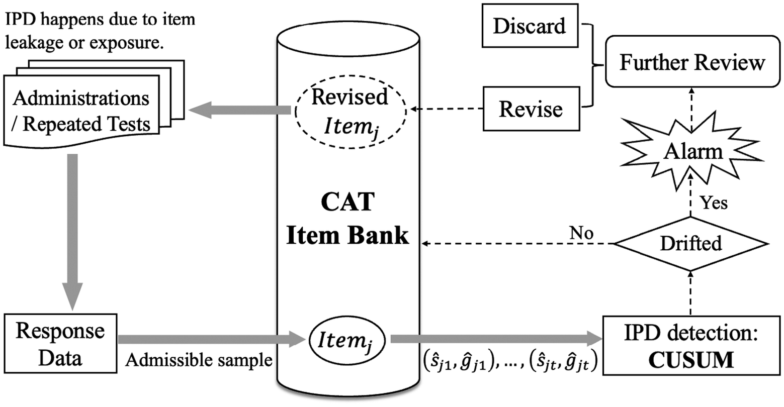
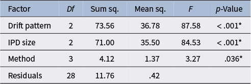

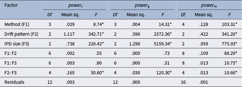
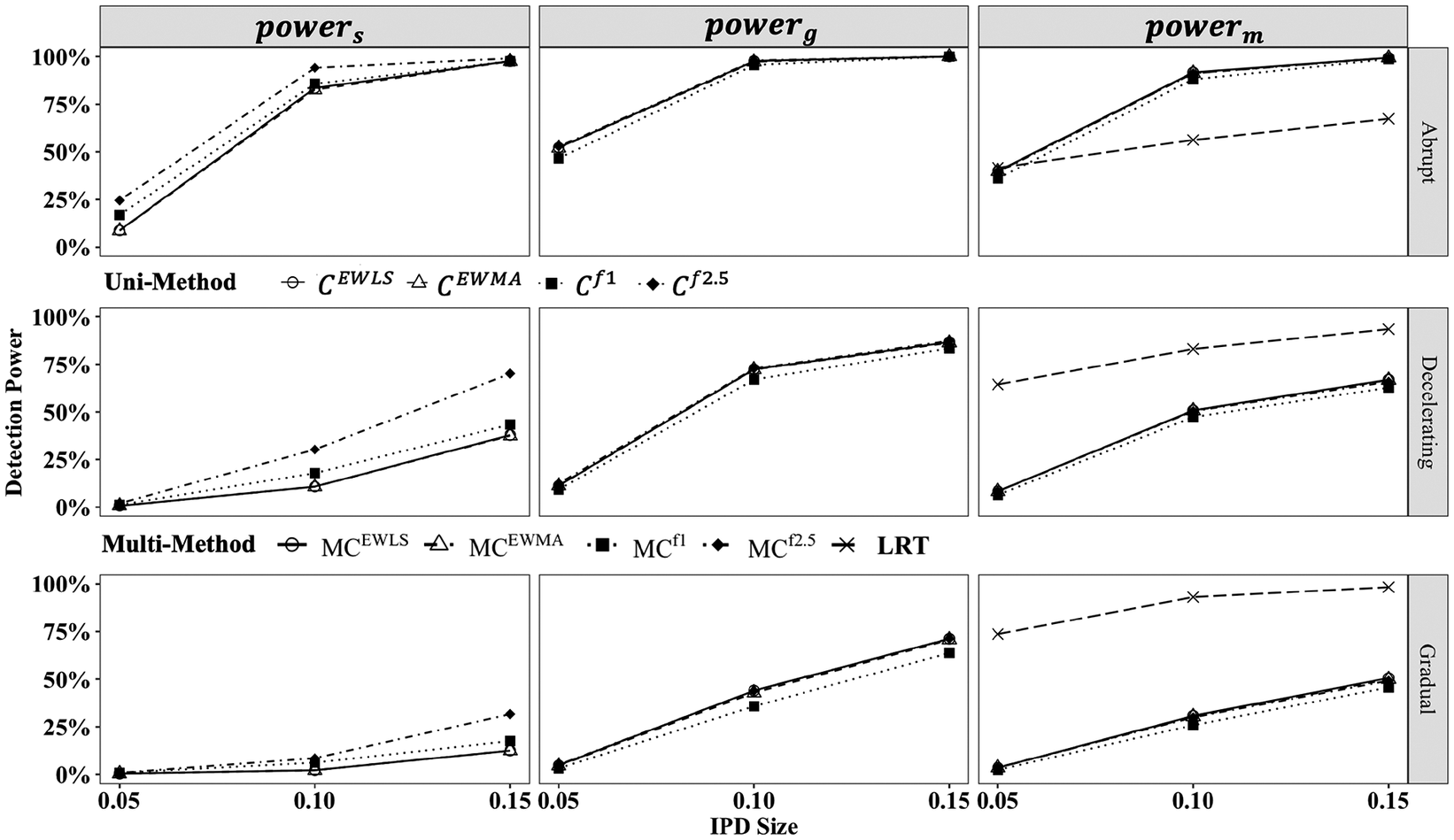
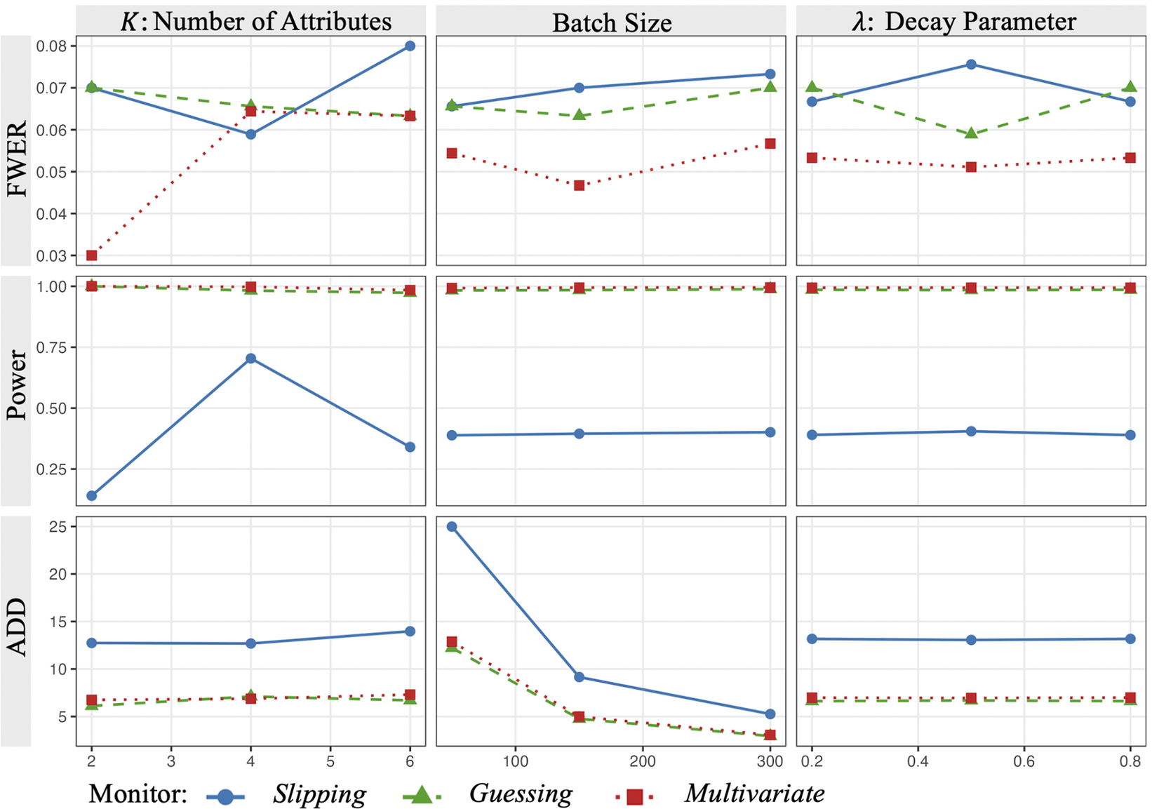


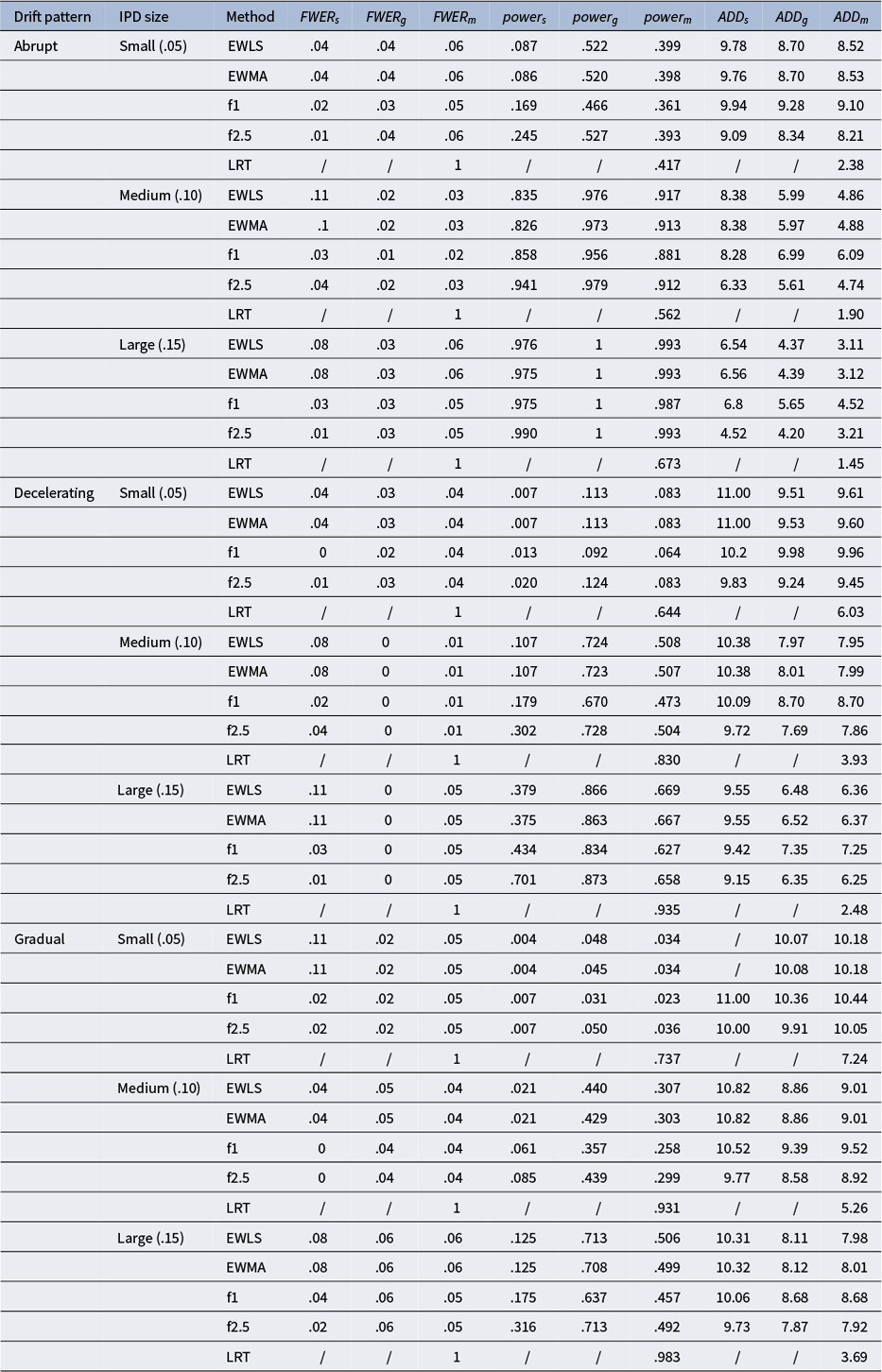
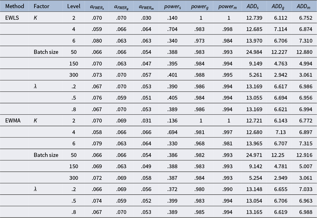


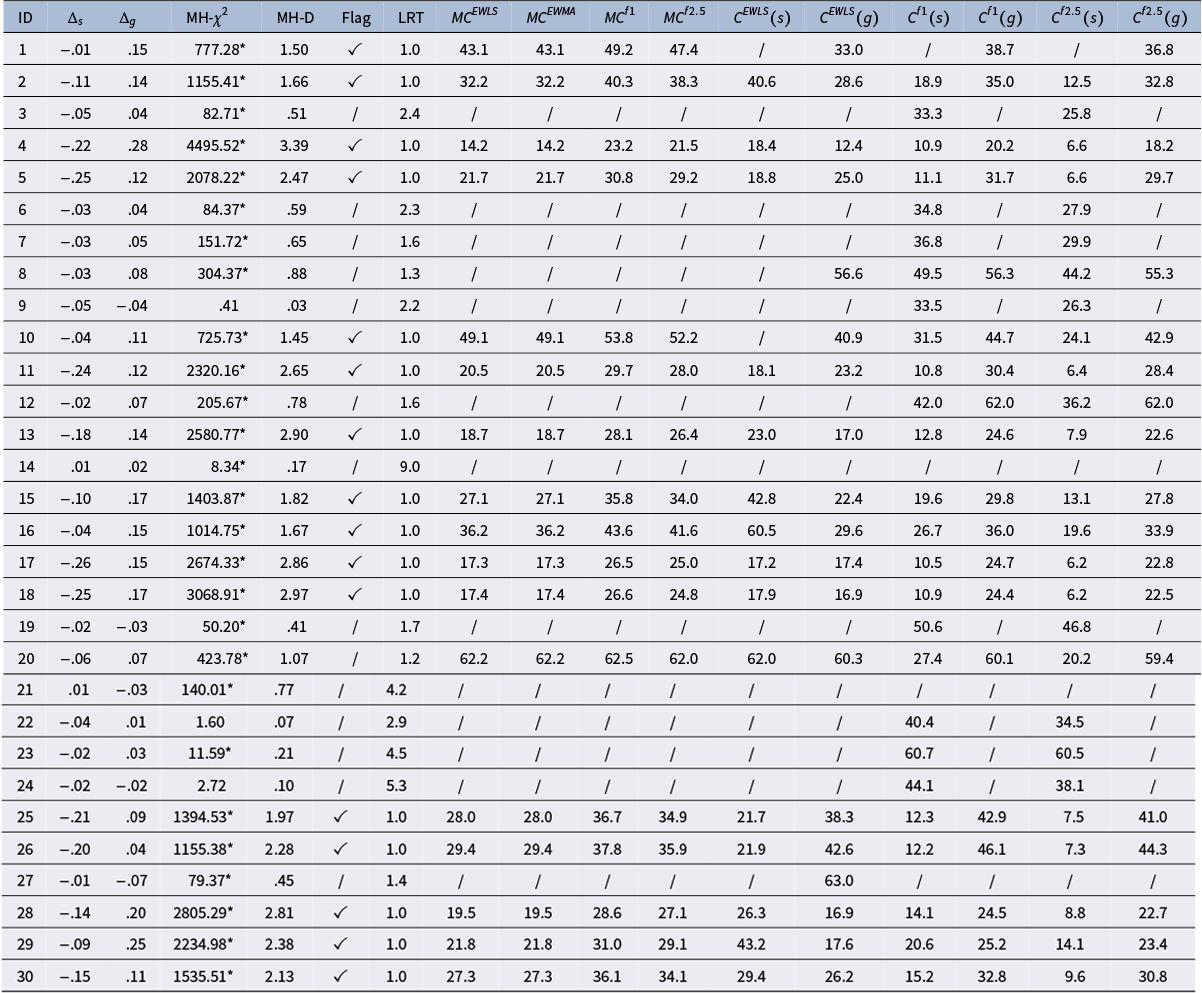


 Open access

