


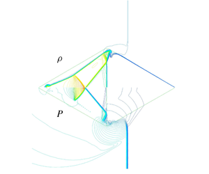
1 Introduction
Shock wave interaction with bubbles of different shapes, containing different gases, results in complex wave patterns. This includes shock wave reflection, refraction and production of vortices. Depending on the contents of the bubble, different types of shock wave interaction can occur, such as slow/fast or fast/slow, as reported by Abd-El Fattah & Henderson (Reference Abd-El Fattah and Henderson1978a,Reference Abd-El Fattah and Hendersonb). Studying shock wave interaction with front- and rear-facing triangles containing light and heavy gases is of great importance in understanding the complex shock wave interaction as well as hydrodynamic instabilities and its effect on mitigating or enhancing the colliding shock/blast wave.
Haas & Sturtevant (Reference Haas and Sturtevant1987) investigated experimentally the interaction of a planar, weak shock wave with a single gas bubble containing either helium or R22, a fluorocarbon (CHClF2). In their experiments, the relevant gas was filled into soap bubbles. The evolved waves and the bubble deformation, due to its collision with the oncoming shock waves, were visualized using shadowgraph photography. The resulting wave configurations were predicted by geometrical acoustics, including the effects of refraction, reflection and diffraction, and were compared with the recorded observations. Also, the pressure field along the bubble’s symmetry axis was recorded by piezoelectric pressure transducers. Bubbles of different geometry were investigated, specifically cylindrical and spherical shapes. In both cases the bubbles were filled with a heavy, low-sound-speed gas or a light, high-sound-speed gas. Different wave structures and bubble deformations were witnessed when using the two different gases inside the investigated bubbles. However, due to the relatively small shock tube test section (8.9 cm cross-section) and the relatively large bubble diameters (4.5 cm), blockage effects are important and the corrections needed were not employed in Haas & Sturtevant (Reference Haas and Sturtevant1987).
Later, Quirk & Karni (Reference Quirk and Karni1996) presented a detailed numerical study of the interaction between a planar weak shock wave with a cylindrical gas bubble based on the experimental results of Haas & Sturtevant (Reference Haas and Sturtevant1987). The obtained simulations were compared with the Haas & Sturtevant (Reference Haas and Sturtevant1987) experimental findings, in which a Mach 1.22 planar shock wave, moving in air, impinges on a cylindrical bubble that contained either helium or R22. The resulting flow field was modelled using the two-dimensional compressible Euler equations for a two-component gas (air–helium or air–R22). Fairly good agreement was found between the experiments and their simulations.
Haas & Sturtevant (Reference Haas and Sturtevant1987) employed the soap film technique for studying the shock–bubble interaction. This technique was adopted by other researchers for generating a spherical gas interface with or without support (e.g. Hosseini & Takayama Reference Hosseini and Takayama2005; Ranjan et al. Reference Ranjan, Anderson, Oakley and Bonazza2005, Reference Ranjan, Niederhaus, Oakley, Anderson, Bonazza and Greenough2008; Layes, Jourdan & Houas Reference Layes, Jourdan and Houas2009; Zhai et al. Reference Zhai, Si, Luo and Yang2011; Haehn et al. Reference Haehn, Ranjan, Weber, Oakley, Rothamer and Bonazza2012; Si et al. Reference Si, Zhai, Luo and Yang2012).
In recent years, several researchers have investigated shock wave interaction with bubbles of different shapes, either a sphere or a cylinder. Some of these bubbles were polygons while others were elliptic. Luo et al. (Reference Luo, Wang, Si and Zhai2015) studied the interaction between a planar shock wave, propagating in air, with a polygonal interface containing sulfur hexafluoride (SF6) gas. Zhai et al. (Reference Zhai, Wang, Si and Luo2014) investigated the case where a shock wave propagating in a heavy gas (SF6) collides with a polygonal bubble containing nitrogen (N2) gas. In such interactions, complex wave patterns are observed, such as regular and irregular refractions, a transmitted shock wave and its reflections, as well as a Mach stem and mutual shock collisions and reflections. In Zhai et al. (Reference Zhai, Wang, Si and Luo2014) the flow field was also solved numerically using the two-dimensional compressible Euler equations for a two-component fluid. Good agreement was obtained with experimental results.
Zhang et al. (Reference Zhang, Zou, Zheng and Wang2019) studied, numerically, the interaction of a weak shock wave with an elliptic cylinder of gas. Three gas pairs having different Atwood numbers were considered: carbon dioxide (CO2) in air (air–CO2), sulphur hexafluoride in air (air–SF6) and krypton (Kr) in helium (He–Kr); all investigated bubbles had a cylindrical shape. For each gas pair, the bubble’s cylinder aspect ratio ranged from 1/4 to 4. Special attention was given to the bubble’s aspect ratio effects on the resulting wave patterns and circulation. Zou et al. (Reference Zou, Liao, Liu, Wang and Zhai2016) investigated experimentally the evolution of a heavy gas (SF6) cylindrical bubble accelerated by a planar weak shock wave. Experiments were conducted with bubbles having five different aspect ratios. It was shown that, as the aspect ratio increases, the interface morphology develops faster owing to larger vortex production along the interface and reduction in the spacing between the two vortex cores.
Schematic description of the double-triangle bubble set-up.

In the present study, a numerical investigation is conducted on the interaction process between a planar shock wave propagating in air with a polygonal bubble composed of two triangles containing SF6 in the front triangle and He in the rear one; see figure 1. Thereafter, the opposite arrangement is studied, i.e. He in the front triangle and SF6 in the rear one. The reliability of the currently employed physical model and its numerical solution was demonstrated in Igra & Igra (Reference Igra and Igra2018). It was shown there that good agreement was achieved with the experimental findings of Luo et al. (Reference Luo, Wang, Si and Zhai2015), obtained for a shock wave interaction with a square and/or triangular bubble containing SF6. This good agreement can be seen in figure 2 of Igra & Igra (Reference Igra and Igra2018), where numerical simulations are compared with schlieren photos taken from Luo et al. (Reference Luo, Wang, Si and Zhai2015). In addition, in figure 3 of Igra & Igra (Reference Igra and Igra2018), a comparison is presented between the experimentally deduced shock wave trajectories of Luo et al. (Reference Luo, Wang, Si and Zhai2015) and its appropriate simulations. It is apparent from figures 2 and 3 in Igra & Igra (Reference Igra and Igra2018) that very good agreement exists between the two findings. Based on this agreement, we have proceeded to investigate the interaction of a planar shock wave propagating in air with the polygonal bubble shown in figure 1 containing two different gases (SF6 and He) having different molecular weights, different specific heat ratios and different acoustic impedances. The density ratio prior to the arrival of the incident shock wave of the light and heavy gases is quite large, almost two orders of magnitude. In all figures shown subsequently, a fixed polygon represents the initial location and shape of the bubble prior to its interaction with the oncoming planar shock wave.
2 Numerical scheme
The computational domain is two-dimensional. Computations were performed using a compressible inviscid flow model. In the considered cases, due to the relatively short flow duration of less than 1 ms, friction and heat transfer losses can be neglected and therefore the Euler equations for mass, momentum and energy conservation were solved. In addition, the species mass fractions for He and SF6 were solved as well. For each gas the appropriate  $\unicode[STIX]{x1D6FE}$ and molecular weight were employed. The mixture properties in each grid cell are based on the local mass fraction of the gases. This method is similar to that employed in Zhai et al. (Reference Zhai, Wang, Si and Luo2014). Simulations were conducted using a second-order Roe upwind scheme.
The solver is second order in both space and time. The mesh is an unstructured type based on quadrilateral cells. It does not change during computation. The grid was constructed in such a way that a lot of cells were located around and inside the triangular gas bubbles. The flow was solved using a finite volume scheme. The conservation equations of mass, momentum and energy were solved in each cell for unsteady flow.
The grid contained 124 580 cells; most were clustered around the bubble boundaries. The computations were conducted on the top half of the flow field shown in figure 1.
A detailed comparison of this numerical scheme with experimental results for shock wave interaction with square and triangular bubbles containing SF6 was presented in Igra & Igra (Reference Igra and Igra2018), where good agreement was obtained for shock wave structures, positions and bubble deformations.
The pre-shock pressure and temperature in the present computations are  $T=298~\text{K}$ and
 $P=101\,325~\text{Pa}$, the same as those used in our previous research (Igra & Igra Reference Igra and Igra2018). The incident shock-wave Mach number was 1.17 and the flow conditions behind the incident shock wave were:
 $u_{2}=90.9~\text{m}~\text{s}^{-1}$,
 $P_{2}=144\,930~\text{Pa}$ and
 $\unicode[STIX]{x1D70C}_{2}=1.52~\text{kg}~\text{m}^{-3}$.
3 Results and discussion
We begin with the case where the front triangle contains SF6 and the rear one He. The results obtained are presented in figures 2–8; they show the interaction process for a planar shock wave propagating in ambient air. Each figure shows the interaction process at a different time. Time counting starts when the incident shock wave impinges upon the apex of the leading triangle. In the figures, on the left (panels a) are lines of constant density and on the right (panels b) are lines of constant pressure. At early time ( $t=108~\unicode[STIX]{x03BC}\text{s}$), shown in figure 2, one sees the incident shock wave over the front triangle containing SF6. The relatively high pressures prevailing behind the propagating incident shock wave deform the triangular bubble’s leading edge and transmit a shock wave into the bubble. As expected, the transmitted shock inside the SF6 bubble (shown in green-yellow colour) is slower than the incident shock wave propagating in air; and upon reaching the bubble’s geometric symmetry line it reflects back towards the bubble’s external surface. As mentioned, due to the head-on collision between the incident shock wave and the triangular bubble’s leading edge, the bubble’s leading edge is deformed to a curved leading edge; see the isopycnal lines shown in figure 2. At this early time, the He gas contained in the rear triangle is unaffected. With ongoing time, the incident shock wave reaches the membrane separating the two gases; the prevailing wave’s structure at the considered time (
 $t=155~\unicode[STIX]{x03BC}\text{s}$) is shown in figure 3. It is apparent from figure 3 that the transmitted shock wave is still inside the front triangle containing SF6. One edge of this oblique shock wave is attached to the incident shock wave propagating in air, and its other edge is travelling along the bubble’s symmetry line. Its top part is the first to reach the rear bubble containing He.
Wave pattern at  $t=108~\unicode[STIX]{x03BC}\text{s}$: (a) lines of constant density, and (b) lines of constant pressure.

Wave pattern at  $t=155~\unicode[STIX]{x03BC}\text{s}$: (a) lines of constant density, and (b) lines of constant pressure.

Therefore, the shock wave motion in the He portion of the bubble is quite different from the previously studied case (Igra & Igra Reference Igra and Igra2018) where a planar shock wave collides head-on with the bubble’s interface. The incident shock wave has just passed the membrane separating the two gases and starts sending compression waves into the He gas. The difference between flow-field presentation via lines of constant density or constant pressure becomes pronounced with increasing time, as is evident from figure 4. It is apparent in figure 4 that the fastest wave propagation is in the He gas where a transmitted compression wave starts its propagation from the top corner of the He triangle towards the symmetry line. As mentioned earlier, the compression waves in the He gas resulted from the relatively high pressure prevailing behind the incident shock wave. Owing to the higher speed of sound in He, these compression waves propagate faster than the incident shock wave (in air), sending compression waves into the ambient air ahead of the incident shock wave; see figure 4 (these behave as precursor shock waves). Owing to the relatively low initial density of the He compared with air and SF6, the waves in the He bubble are not visible in the density contours. At the considered time ( $194~\unicode[STIX]{x03BC}\text{s}$) the top of the transmitted shock wave in SF6 that impinged upon the SF6–He interface is reflected back from the apex of the SF6–He interface towards the leading edge of the SF6 bubble, while the lower section of the transmitted shock wave in SF6 continues to propagate towards the He bubble rear sharp edge. With elapsed time (
 $t=285~\unicode[STIX]{x03BC}\text{s}$) the incident shock wave is approaching the bubble trailing edge while the compression wave in the He gas is already reflected back towards the membrane separating the two gases. During its travel it transmits a compression wave into the air ahead and behind the incident shock wave.
Wave pattern at  $t=194~\unicode[STIX]{x03BC}\text{s}$: (a) lines of constant density, and (b) lines of constant pressure.

In addition, at the considered time ( $t=285~\unicode[STIX]{x03BC}\text{s}$) the slow propagating transmitted shock wave that was reflected from the symmetry line in the SF6 gas has been reduced to a compression wave and reaches the membrane separating the two gases. The meeting of all these compression waves generates a vortex that further deforms the bubble’s surface near the membrane separating the two gases; see figure 5. At the considered time (
 $t=285~\unicode[STIX]{x03BC}\text{s}$) the reflection of the transmitted shock wave from the bubble symmetry line exhibits a clear Mach reflection pattern. With progressing time (
 $t=327~\unicode[STIX]{x03BC}\text{s}$) the bubble further deforms.
Wave pattern at  $t=285~\unicode[STIX]{x03BC}\text{s}$: (a) lines of constant density, and (b) lines of constant pressure.

At the bubble leading edge, a new vortex evolves mixing SF6 with the external air. The intensity of the vortex in the He section intensifies; it mixes He, SF6 and air and the transmitted shock wave is at its final diffraction over the bubble as shown in figure 6. At  $t=327~\unicode[STIX]{x03BC}\text{s}$ the bubble deformation continues, as is evident from figure 6. The vortex in the He section, seen first in figure 5, intensifies and so does the pressure seen on the symmetry line, at the SF6 section near the Mach reflection in figure 5; it increases in figure 6. A clear description of the mixing can be seen in figure 7 where contours of
 $\unicode[STIX]{x1D6FE}$ and mass fractions of air, He and SF6 are presented. It is apparent in figure 7 that there are two mixing vortices near the two gas interfaces, the upper one (shown in green-blue colour and marked by an arrow in figure 7a) mixes all three gases while the second vortex (in orange colour and marked by an arrow in figure 7c) mixes air and He. Additional details can be seen in the mass fractions shown in figure 7.
Wave pattern at  $t=327~\unicode[STIX]{x03BC}\text{s}$: (a) lines of constant density, and (b) lines of constant pressure.

Contours at  $t=327~\unicode[STIX]{x03BC}\text{s}$: (a)
 $\unicode[STIX]{x1D6FE}$ contour plot, (b) air mass fraction, (c) He mass fraction, and (d) SF6 mass fraction.

While, thus far, in spite of the pronounced deformation of the original bubble geometry, it has been possible to observe two closed regions containing different gases, at a later time this is not the case, as is evident from figure 8 showing the situation at  $t=640~\unicode[STIX]{x03BC}\text{s}$. At that time, the SF6 part of the bubble is separated from the He part. Additional vortices appear on the front surface of the SF6 part of the bubble, advancing its mixing with the external air; see figure 8(a). The upstream propagation of the reflected shock from the separating membrane continues and a distorted Mach reflection of this weak shock from the bubble symmetry line is clearly seen in figure 8(b). At the considered time, the He part of the bubble is in the later part of the process of being completely mixed with the surrounding air, as seen in figure 8. The vortex seen at earlier times in the He section is still active and continues diluting the He content by mixing it with the external air.
Wave pattern at  $t=640~\unicode[STIX]{x03BC}\text{s}$: (a) lines of constant density, and (b) lines of constant pressure.

The deformation of the SF6 bubble’s section is similar to that seen in the schlieren photo shown in figure 6 of Luo et al. (Reference Luo, Wang, Si and Zhai2015) obtained for a forward-facing triangular bubble. However, in their experiments, the bubble was filled mostly with SF6 but contained some air and the incident shock wave is slightly different from the current case.
It is of interest to determine whether or not changes in the gas location, shown in figure 1, i.e. placing the He gas in the front triangle and SF6 in the rear one, will result in meaningful changes in the evolved flow field. To answer this question, the present simulation was repeated for the case in which the bubble’s front section contained He while its rear section was filled with SF6. The initial flow conditions were the same as in the previous case, i.e. pre-shock pressure and temperature of  $P=101\,325~\text{Pa}$ and
 $T=298~\text{K}$, respectively, and the incident shock wave Mach number was 1.17.
In figures 9–27, the interaction process for this reversed case between a relatively weak incident shock wave ( $M=1.17$) and the bubble whose shape is shown in figure 1 is investigated. Time counting starts when the incident shock wave hits the bubble’s leading edge. The results shown in figure 9 show the early time (
 $t=14~\unicode[STIX]{x03BC}\text{s}$) of the shock diffraction over the bubble. As before, in figure 9(a) one sees lines of constant density and thereby the bubble’s surface; in figure 9(b) one sees lines of constant pressure.
Wave pattern at  $t=14~\unicode[STIX]{x03BC}\text{s}$: (a) lines of constant density, and (b) lines of constant pressure.

The straight lines in all the figures indicate the original bubble’s shape and location. As expected, upon the head-on collision between the incident shock wave and the bubble’s leading edge (i.e. the bubble’s apex-sharp leading edge) is deformed and a compression wave is transmitted into the He gas contained in the bubble front section. As the speed of sound in He is higher than in air, the front of the compression wave is seen in figure 9 ahead of the incident shock wave. This creates a precursor shock wave in the ambient air that is connected with the front of the compression wave seen in the He bubble. With progressing time ( $t=37~\unicode[STIX]{x03BC}\text{s}$) the bubble deformation increases and the compression wave continues its propagation towards the interface separating the two gases; see figure 10. In addition, the transmitted compression wave inside the He gas transmits a compression wave ahead of the incident shock wave, as is clearly seen in figure 10.
Wave pattern at  $t=37~\unicode[STIX]{x03BC}\text{s}$: (a) lines of constant density, and (b) lines of constant pressure.

At  $t=54~\unicode[STIX]{x03BC}\text{s}$ the transmitted compression wave in the He gas approaches the membrane separating the two gases. While propagating upstream, the precursor zone ahead of the incident shock wave is enlarged due to the velocity difference between the shock wave in air and in He. Its direction of propagation is both downstream and opposite to the symmetry line. A regular reflection of the incident shock wave from the bubble surface is observed in figure 11. A short time later, at
 $t=59~\unicode[STIX]{x03BC}\text{s}$, the front of the transmitted compression wave reaches the membrane separating the two gases; see figure 12. From this time on, a reflected shock wave will be transmitted upstream (towards the bubble leading edge) and a compression wave will be transmitted into the SF6.
Wave pattern at  $t=54~\unicode[STIX]{x03BC}\text{s}$: (a) lines of constant density, and (b) lines of constant pressure.

Wave pattern at  $t=59~\unicode[STIX]{x03BC}\text{s}$: (a) lines of constant density, and (b) lines of constant pressure.

At  $t=64~\unicode[STIX]{x03BC}\text{s}$ the reflection of the transmitted compression waves from the membrane separating the two gases is almost completed, see figure 13, and the initiation of a transmitted shock wave into the SF6 gas is visible in figure 13(b). At the considered time, while the deformation of the bubble’s He section continues, the SF6 section of the bubble still keeps its original shape.
Wave pattern at  $t=64~\unicode[STIX]{x03BC}\text{s}$: (a) lines of constant density, and (b) lines of constant pressure.

Thereafter ( $t=79~\unicode[STIX]{x03BC}\text{s}$, figure 14) the weak shock wave transmitted into the SF6 section of the bubble is slowly propagating towards the bubble’s trailing edge, leaving behind it an area of non-uniform pressure. In the considered time, while the incident shock wave is still on its way towards the interface separating the two gases, the precursor shock wave from the compressed He, ahead of the incident shock wave, has passed this location, as is evident in figure 14.
Wave pattern at  $t=79~\unicode[STIX]{x03BC}\text{s}$: (a) lines of constant density, and (b) lines of constant pressure.

Later, at  $t=122~\unicode[STIX]{x03BC}\text{s}$ shown in figure 15, while the incident shock wave approaches the membrane separating the two gases, the precursor shock wave that was created when the incident shock wave impacted the He section is seen now well ahead of the incident shock wave. Upon its passing the bubble’s corner, at the membrane separating between He and SF6, it experiences expansion that will generate a vortex at this location.
Wave pattern at  $t=122~\unicode[STIX]{x03BC}\text{s}$: (a) lines of constant density, and (b) lines of constant pressure.

An interesting development, whose initiation is hinted in figure 15, becomes clear in figure 16 ( $t=132~\unicode[STIX]{x03BC}\text{s}$). One sees there two clear vortices, one located at the deformed leading edge of the bubble, the second at the recently deformed corner (at the membrane separating the two gases).
Wave pattern at  $t=132~\unicode[STIX]{x03BC}\text{s}$: (a) lines of constant density, and (b) lines of constant pressure.

With increasing time, at  $t=200~\unicode[STIX]{x03BC}\text{s}$, the deformation of the bubble’s He section continues and the vortex initiated at the bubble separation point between the two gases is strengthened, see figure 17. The transmitted shock wave in the SF6 continues propagating downstream; however, it does not propagate into a uniform state, as the precursor shock wave from the He section is travelling ahead of both the incident shock wave propagating in air and the transmitted shock in the SF6 gas; see the pressure contour of figure 17.
Wave pattern at  $t=200~\unicode[STIX]{x03BC}\text{s}$: (a) lines of constant density, and (b) lines of constant pressure.

At a later time,  $t=238~\unicode[STIX]{x03BC}\text{s}$, the vortex seen over the bubble intensifies, thereby enhancing mixing between SF6, He and air. The upper part of the transmitted shock wave in the SF6 gas weakens due to its interaction with the precursor shock wave from the He gas; see figure 18. Owing to this interaction, a shock splitting is seen in figure 18 near the bubble surface.
Wave pattern at  $t=238~\unicode[STIX]{x03BC}\text{s}$: (a) lines of constant density, and (b) lines of constant pressure.

A clear view of the evolved mixing between the gases is shown in figure 19, where contours of  $\unicode[STIX]{x1D6FE}$ and mass fractions of air, He and SF6 are shown. The vortices seen at the upper surface (marked by an arrow in figure 19a) separating He and SF6 intensively mixes the three gases, air, He and SF6. It is also apparent that the two vortices rotate in opposite directions. It is also shown in figure 19 that, while the front vortex mixes He and air, the upper one mixes all three gases as shown in the mass fraction contours.
Contours at  $t=238~\unicode[STIX]{x03BC}\text{s}$: (a)
 $\unicode[STIX]{x1D6FE}$ contour plot, (b) air mass fraction, (c) He mass fraction, and (d) SF6 mass fraction.

Similar shock wave structures were reported in Luo et al. (Reference Luo, Wang, Si and Zhai2015) and in Igra & Igra (Reference Igra and Igra2018) for shock wave interaction with a backward-facing triangular bubble. This is due to the fact that the compression waves in the He impacted the rear of the SF6 bubble almost like a planar shock wave, as reported in previous research. This is different from the previously discussed case where the shock wave impacting on the rear bubble containing He had a completely different shape due to its propagation in the SF6 bubble.
A short time later, at  $t=248~\unicode[STIX]{x03BC}\text{s}$, the upper vortex intensifies while the vortex that began at the original bubble apex weakens; see figure 20. The incident shock wave also weakens, and close to the bubble surface it is reduced to a compression wave initiated by a precursor shock wave emanating from the He gas. By now (
 $t=248~\unicode[STIX]{x03BC}\text{s}$) the He section is dramatically deformed relative to its original shape while the SF6 section still maintains some resemblance to its original geometry; see figure 20. This process continues, as is evident from figure 21, showing the situation at
 $t=273~\unicode[STIX]{x03BC}\text{s}$. Now the incident shock wave is approaching the bubble’s trailing edge and the transmitted shock wave in the SF6 is composed of two parts. One part maintains its original direction, propagating downstream, while the second propagates in a vertical direction, towards the bubble’s symmetry line.
Wave pattern at  $t=248~\unicode[STIX]{x03BC}\text{s}$: (a) lines of constant density, and (b) lines of constant pressure.

Wave pattern at  $t=273~\unicode[STIX]{x03BC}\text{s}$: (a) lines of constant density, and (b) lines of constant pressure.

A similar shock wave structure was reported in Luo et al. (Reference Luo, Wang, Si and Zhai2015) and in Igra & Igra (Reference Igra and Igra2018). The vortex seen earlier near the bubble’s symmetry line weakens significantly and its interaction with the separation surface separating the two different gases results in a local area of relatively high pressure; see the red spot in figure 21. At  $t=307~\unicode[STIX]{x03BC}\text{s}$ the vortex observed previously in the He section near the bubble symmetry line is pushed now into the SF6 section, intensifying mixing between the two gases. The part of the transferred shock wave inside the SF6 gas that progresses along the bubble symmetry line becomes shorter while the part progressing towards the bubble symmetry line is reduced to a compression wave, as is evident from figure 22.
Wave pattern at  $t=307~\unicode[STIX]{x03BC}\text{s}$: (a) lines of constant density, and (b) lines of constant pressure.

A short time later, at  $t=343~\unicode[STIX]{x03BC}\text{s}$, the compression wave that propagated towards the bubble symmetry line is reflected back from the symmetry line and it raises the local pressure behind it; see the red zone in figure 23. With progressing time (
 $t=461~\unicode[STIX]{x03BC}\text{s}$) both sections of the original bubble are significantly deformed, resulting in initiation of new vortices turning the entire flow field into highly turbulent flow, as is evident from figure 24.
Wave pattern at  $t=343~\unicode[STIX]{x03BC}\text{s}$: (a) lines of constant density, and (b) lines of constant pressure.

Wave pattern at  $t=461~\unicode[STIX]{x03BC}\text{s}$: (a) lines of constant density, and (b) lines of constant pressure.

The local high-pressure zone seen earlier (in figure 23) at the bubble symmetry line now moves away from this line; it appears as a small red spot in the SF6 region in figure 24. The bubble distortion and the vortices strengthening become more pronounced with increasing time, as is evident from figure 25. Now the small (red colour) pressure zone seen in figure 24 moves slightly downstream and becomes a shock wave; see figure 25.
Wave pattern at  $t=637~\unicode[STIX]{x03BC}\text{s}$: (a) lines of constant density, and (b) lines of constant pressure.

At  $t=637~\unicode[STIX]{x03BC}\text{s}$ most of the He gas is mixed with the ambient air and the He section of the original bubble is hardly visible. The shock wave seen earlier weakens and, due to the strengthening of the vortices inside and outside of the SF6 section of the bubble, it moves downstream and closer to the symmetry line; see figure 25.
A description of the mixing between the involved gases is shown in figure 26, where contours of  $\unicode[STIX]{x1D6FE}$ and mass fractions of air, He and SF6 are shown. The mixing can be clearly seen in the
 $\unicode[STIX]{x1D6FE}$ contour plot displaying large change in its value. In figure 26(c) the He mass fraction contour is shown; it is observed as small islands in the surrounding air and large parts of it are mixed with the surrounding gases. The interaction process approaches its end at
 $t=706~\unicode[STIX]{x03BC}\text{s}$. At this time the weak shock wave seen earlier turns into a relatively high-pressure zone inside the remaining small area of the original SF6 section of the bubble; see figure 27.
Contours at  $t=637~\unicode[STIX]{x03BC}\text{s}$: (a)
 $\unicode[STIX]{x1D6FE}$ contour plot, (b) air mass fraction, (c) He mass fraction, and (d) SF6 mass fraction.

Wave pattern at  $t=706~\unicode[STIX]{x03BC}\text{s}$: (a) lines of constant density, and (b) lines of constant pressure.

It is of interest to compare the two different flow fields resulting from the interaction between a planar shock wave propagating in air ( $M=1.17$) with either a polygonal bubble containing SF6–He or He–SF6. In figure 28 the shock trajectories of the incident shock wave (isw), the transmitted shock wave (tsw) and the incident shock wave locations along the bubble interface (sb) are presented. In figure 29 the trajectories of the bubble’s leading edge, centre and trailing edge location are shown for the two different cases.
Trajectories of the incident shock wave (isw), the shock along the bubble perimeter (sb) and the transmitted shock wave (tsw).

Movement of the bubble’s leading edge, centre and trailing edge.

In the case when the bubble’s front triangle contains SF6, during most of the time shown in figure 28 the transmitted shock wave is still propagating inside the SF6 section until approximately  $155~\unicode[STIX]{x03BC}\text{s}$ and therefore it exhibits a constant, low speed; see figure 28. This is clearly seen in the isw and tsw. However, in the case of sb, once it reaches the He in the rear of the bubble it accelerates quickly (for
 $t>155~\unicode[STIX]{x03BC}\text{s}$). In the case of
 $\text{He}\rightarrow \text{SF}_{6}$ the transmitted shock wave propagates much faster in the He gas and therefore it experiences two different velocities during its travel through the bubble. First there is a quick propagation through the He section of the bubble and, thereafter, a slow propagation in the bubble’s SF6 section. Based on the results shown in figure 28, the velocities of the different waves can be computed; these are presented in table 1.
Wave velocities for different bubbles.

The rate of bubble deformation can be concluded from the trajectories shown in figure 29. In the SF6–He case the bubble’s leading, centre and trailing edges exhibit three different velocities. During the investigated time, the bubble’s leading edge is affected mostly by the pressure behind the reflected shock wave from the bubble and the pressure prevailing behind the slow transmitted shock wave in the SF6 gas. As a result, it exhibits a slow movement, at almost constant velocity. The velocities approximated from figure 29 are shown in table 2.
Velocities for bubble’s front rear and centre.

The bubble’s centre and trailing edge show no displacement until the transmitted shock wave reaches the bubble’s centre (the location of the interface separating the two gases). Once the transmitted shock wave enters the He section, a significant acceleration, downstream of the bubble’s centre and trailing edge, is evident; see figure 29. A significantly different behaviour is seen in the He–SF6 case. Now, due to the very quick propagation of the transmitted shock wave in He after a short time, approximately  $270~\unicode[STIX]{x03BC}\text{s}$, both the bubble’s leading edge and centre points propagate downstream at the same velocity; see figure 29.
Next, we compare the prevailing pressures for the two different gas arrangements inside the bubble, SF6–He and He–SF6. The obtained results of computed pressure along the bubble symmetry line are shown in figure 30. In addition, the initial locations of the bubble’s leading and trailing edges and the two gas interfaces are marked by dashed lines in figure 30. It is apparent from this figure that higher pressures are experienced in the SF6–He configuration. Furthermore, while in the He–SF6 case a clear transmitted shock wave is visible, in the SF6–He case a compression wave is visible ahead of the transmitted shock wave.
Pressure variations at different times during the incident shock wave interaction with a polygonal bubble containing two different gases.

It is apparent in figure 30 that in the He–SF6 configuration, during the flow times  $t=122$ and
 $132~\unicode[STIX]{x03BC}\text{s}$, a pronounced unsteady flow region exists in the small areas before and after the interface separating the two gases (
 $0.01<x<0.06~\text{m}$). This was already seen in figures 15 and 16 showing the flow field for the considered time period. As already mentioned, in figure 16 one sees two clear vortices: one at the deformed leading edge of the bubble, and the second at the deformed corner above the interface separating the two gases. The blue line seen in figure 16(a) indicates the borders of the bubble’s He section; its right border appears as a green line in figure 16(b). The pressure encountered in the SF6 bubble was higher than that found in the He bubble for both types of bubbles considered in the current study. When the front portion of the bubble contained SF6, its maximal pressure was approximately 50 % higher than in the case when it was placed in the rear bubble due to the fact that it initially absorbed the incoming incident shock wave.
4 Conclusions
The interaction between a planar shock wave propagating in air with a polygonal bubble containing two different gases was studied numerically. It is shown that, due to the large differences in molecular weight, specific heat ratio and acoustic impedances between the investigated gases, a complex wave pattern developed during the interaction. The wave motion in the rear portion of the bubble is strongly affected by the gas type in the front portion of the bubble and the propagation of the transmitted shock wave inside it. The final bubble shape of the cases studied is quite different and the bubble content affects the outcome. The wave propagation in the SF6 section of the bubble is significantly slower than that witnessed in the He section. Therefore, it is affected not only by the diffraction of the incident shock wave over it, but also by pressure transmitted ahead of the incident shock wave, upstream from the He section. The pressures in the SF6 part of the bubble were higher than those found in the He section of the bubble, for both bubbles computed in the current study. When the front bubble contained SF6, its maximum pressure was approximately 50 % higher than that found in the case when it was placed in the rear portion of the bubble.



