1. Introduction
With the development of high-speed aircraft, there is growing concern over the laminar–turbulent transition. As roughness-induced transition is one of the main forms of transition for high-speed vehicles, its control is of great importance for the reduction of surface heat flux and friction drag (Lin Reference Lin2008; Estruch-Samper et al. Reference Estruch-Samper, Hillier, Vanstone and Ganapathisubramani2017). To obtain an effective approach for the control of roughness-induced transition, its mechanism should first be understood. However, although massive efforts have been made, it is still not well known, and a substantial amount of work needs to be done (Schneider Reference Schneider2015). Early researchers (Smith & Clutter Reference Smith and Clutter1959) indicated that whether or not the transition occurs downstream depends on the properties of the boundary layer at the maximum height of roughness element  $k_r$, and, therefore, the roughness Reynolds number
 $Re_{kk}$ was defined to predict transition:
 \begin{equation} Re_{kk}=\frac{\rho_k u_k k_r}{\mu_k}. \end{equation}
Here  $\rho$,
 $u$ and
 $\mu$ are density, streamwise velocity and dynamic viscosity, respectively, and subscript
 $k$ represents quantities measured at
 $k_r$. The transition onset position will rapidly approach the roughness when
 $Re_{kk}$ exceeds a critical value (Puckert & Rist Reference Puckert and Rist2018). While the roughness Reynolds number is an effective criterion for transition prediction in cases where the roughness element is overwhelmed by the boundary layer (Bernardini et al. Reference Bernardini, Pirozzoli, Orlandi and Lele2014), it remains a phenomenological theory.
Previous attempts to describe the mechanism of roughness-induced transition suggested that the source of unsteadiness varies with the change in flow configuration. There are several main structures in the flow past the roughness element that may introduce disturbance into flow fields. In the upstream separation zone, there is a horseshoe vortex formed wrapping around the front half of the roughness, and then it trails downstream as streamwise vortices (Gregory & Walker Reference Gregory and Walker1956). Baker (Reference Baker1979) conducted a thorough investigation of the horseshoe vortex system in a laminar separation zone upstream of the roughness element. Especially in cases with a high roughness element relative to the boundary layer displacement thickness, complicated unsteady behaviour was found resulting from the instability of the vortex system itself.
In the high-speed boundary layer, a shockwave system exists in front of the roughness. It was observed by Subbareddy, Bartkowicz & Candler (Reference Subbareddy, Bartkowicz and Candler2014) that the vortex system in the separation zone perturbs the shockwave by affecting the compression wave system near the wall. Moreover, disturbance in the downstream wake structure also influences the shockwave through the boundary layer. They indicated that the upstream vortex and shockwave systems are the primary causes of transition occurring downstream of a cylindrical roughness at inflow Mach number  ${Ma}_\infty =6$ (
 $Ma$ is the Mach number, and subscript
 $\infty$ refers to quantities of inflow).
The shear layer shedding from roughness can also be a main contribution to the disturbance growth, as it can create an inflection point in the velocity profile and introduce Kelvin–Helmholtz (KH) instability into the flow field (Ergin & White Reference Ergin and White2006; Semper & Bowersox Reference Semper and Bowersox2017). Hamed et al. (Reference Hamed, Sadowski, Zhang and Chamorro2016) observed in experiments that fluctuation near roughness is related to the shear layer separated from both two-dimensional and three-dimensional periodic roughness, and Chou, Kegerise & King (Reference Chou, Kegerise and King2020) found that the shear layer can induce sinuous or varicose mode instabilities depending on the roughness height.
Except for the shear layer, the wake structure also contains a counter-rotating vortex pair shedding from the top of the roughness element (Gregory & Walker Reference Gregory and Walker1956). The lift-up effect (Landahl Reference Landahl1980; Brandt Reference Brandt2014) allows streamwise vortices in the wake to induce disturbance transient growth (Reshotko Reference Reshotko2001) by distorting the boundary layer profile in the spanwise direction and creating streaks, which is the optimal disturbance in transient growth mechanisms according to the results of theory (Luchini Reference Luchini2000). Experiments performed by White (Reference White2002) and White, Rice & Ergin (Reference White, Rice and Ergin2005) indicated that disturbance undergoes an algebraic transient growth at the position of streamwise vortices behind an isolated roughness element and finally results in transition downstream.
Moreover, the counter-rotating vortex pair can interact with a separated shear layer and bend it to surround the wake (De Tullio et al. Reference De Tullio, Paredes, Sandham and Theofilis2013). As observed by Muppidi & Mahesh (Reference Muppidi and Mahesh2012) in flow at  ${Ma}_\infty =2.9$ past distributed roughness, the interaction between these two structures can lead to the shear layer breaking down into turbulence. In cases with isolated cylindrical roughness, Subbareddy et al. (Reference Subbareddy, Bartkowicz and Candler2014) recognized the interaction as the second dominant mechanism of transition using dynamic mode decomposition (DMD) (Rowley et al. Reference Rowley, Mezić, Bagheri and Schlatter2009; Schmid Reference Schmid2010). Recently, Shrestha & Candler (Reference Shrestha and Candler2019) performed a similar analysis on flow past a diamond-shaped roughness, and suggested that the separated shear layer/counter-rotating vortex interaction is the primary cause for transition in their study.
As roughness-induced transition is a competitive mechanism between the development of unsteady fluctuation and relaxation of flow field distortion (Ergin & White Reference Ergin and White2006), the studies above seem to imply that the roughness-induced transition can be controlled by changing the magnitude of these main structures in the flow field and influencing the growth rate of the disturbance. For example, White et al. (Reference White, Rice and Ergin2005) observed that the change in the roughness configuration alters the vorticity field in the wake structure and affects the disturbance transient growth rate, and Subbareddy et al. (Reference Subbareddy, Bartkowicz and Candler2014) found that the inflow Reynolds number has an important impact on the structure of the horseshoe vortex system in the upstream separation zone and the transition onset position downstream of cylindrical roughness.
Thus, several effective control methods have been proposed to modify the flow configuration of the roughness-disturbed boundary layer. One of them delays transition by placing another roughness element with a specially designed shape at a specific position downstream of the original element, so that the distortion of the boundary layer profile generated by these two elements can counteract each other. This method was first adopted for two-dimensional roughness by Kobayashi et al. (Reference Kobayashi, Fukunishi, Nishikawa and Kato1994) and then applied to the control of three-dimensional roughness (Sharma et al. Reference Sharma, Drews, Kuester, Goldstein and White2014; Suryanarayanan et al. Reference Suryanarayanan, Goldstein, Brown, Berger and White2017). Despite its significant effect, this method only works on roughness with a particular shape. Another method takes effect with some relatively lower roughness around the original one. The phenomenon of this method was first observed by Kendall (Reference Kendall1981) and then employed in the control of the transition induced by distributed (Downs, White & Denissen Reference Downs, White and Denissen2008) and discrete roughness (Kuester & White Reference Kuester and White2015). Lu et al. (Reference Lu, Liu, Liu and Yan2020a,Reference Lu, Liu, Liu and Yanb) analysed the effect of upstream and downstream-positioned control roughness separately and argued that their roles in transition control are different. However, as a passive strategy, it is unable to adjust the control effect. Moreover, the small-amplitude roughness used in this method would not only introduce some additional disturbance into the flow field but also increase surface friction and heat flux, especially in the high-speed boundary layer.
Wall blowing is a widely used and adjustable tool in the control of transition induced by first-mode instabilities (Sharma et al. Reference Sharma, Shadloo, Hadjadj and Kloker2019), and it is reported to have the ability to reduce surface friction drag (Mori, Quadrio & Fukagata Reference Mori, Quadrio and Fukagata2017). Therefore, our aim is to propose a new method for the control of transition induced by roughness using wall blowing. Direct numerical simulation (DNS) is performed in this paper to obtain an accurate flow field of the transition process so that the mechanism of roughness-induced transition and its control with wall blowing can be analysed. Wall blowing located both upstream and downstream of the roughness element is studied separately, as their roles in the control of roughness-induced transition seem to be different. Furthermore, blowing of weak or strong intensity is simulated separately because they have a reverse influence on the transition onset position with the increase in intensity.
This paper is organized as follows. In § 2 we illustrate the set-up of our computations and the validation of our results. Then in § 3 we demonstrate the results of all the cases and our analyses. The mechanism of transition induced by a discrete roughness element is analysed in § 3.1, the role of upstream- or downstream-positioned weak wall blowing in the inhibition of transition is assessed in § 3.2, and the effect of upstream- or downstream-positioned strong wall blowing promoting transition is investigated in § 3.3. Finally, § 4 presents the conclusion of our study.
2. Computation set-up and validation
In this paper, a supersonic free-stream flow condition is considered for all cases. The inflow parameters are described in table 1 (where  $Re_{ref}=\rho _\infty {u}_\infty /\mu _\infty$,
 $T$ represents temperature, subscript
 $w$ denotes flow parameters at the wall, and
 $R$,
 $\gamma$ and
 $Pr$ are the gas constant, heat capacity ratio and laminar Prandtl number, respectively). This condition has been adopted in many studies before (Pirozzoli, Grasso & Gatski Reference Pirozzoli, Grasso and Gatski2004; Li et al. Reference Li, Fu, Ma and Gao2009).
Free-stream flow conditions.

As mentioned in § 1, the roughness Reynolds number  $Re_{kk}$ is a key parameter for roughness-induced transition. In this study, a discrete roughness element is placed at
 $x_r=101.6\ \mathrm {mm}$ (measured from the leading edge of the flat plate). To estimate the maximum height of the roughness element to satisfy the given value of
 $Re_{kk}$, we need to obtain the flow profile at
 $x_r$ in the undisturbed laminar boundary layer. For this purpose, compressible Blasius equations (Stewartson Reference Stewartson1964) are solved with the shooting method and eighth-order Runge–Kutta method (Butcher Reference Butcher2003). The compressible Blasius equations with similarity transformation can be written as
 \begin{equation}
\left.\begin{array}{c@{}} \begin{array}{l@{}} \displaystyle
\dfrac{\textrm{d}}{\textrm{d}\eta_c}
\left(\dfrac{\rho\mu}{\rho_\infty\mu_\infty}\dfrac{\textrm{d}^2f}{\textrm{d}
\eta_c^2}\right)+f\dfrac{\textrm{d}^2f}{\textrm{d}\eta_c^2}=0,\\
\displaystyle \dfrac{\textrm{d}}{\textrm{d}\eta_c}
\left(\dfrac{\rho\mu}{\rho_\infty\mu_\infty}\dfrac{\textrm{d}g}{\textrm{d}\eta_c}\right)+
Pr\,{f}\dfrac{\textrm{d}g}{\textrm{d}\eta_c}+Pr(\gamma-1){Ma}^2_\infty
\dfrac{\rho\mu}{\rho_\infty\mu_\infty}\dfrac{\textrm{d}^2f}{\textrm{d}\eta_c^2}=0,
\end{array} \\
\displaystyle
f(0)=\left.\frac{\textrm{d}\,f}{\textrm{d}\eta_c}\right|_{\eta_c=0}=0,
\quad g(0)=\frac{T_w}{T_\infty}, \quad
\lim_{\eta_c\rightarrow+\infty}\frac{\textrm{d}f}{\textrm{d}\eta_c}=
\lim_{\eta_c\rightarrow+\infty}g(\eta_c)=1,
\end{array}\right\}
\end{equation}
where
 \begin{equation} \frac{\textrm{d}f}{\textrm{d}\eta_c}=\frac{u}{u_\infty},\quad g=\frac{T}{T_\infty},\quad \eta_c=\sqrt{\frac{\rho_\infty{u}_\infty}{2\mu_\infty{x}}} \int^y_0\frac{\rho}{\rho_\infty}\,\textrm{d} y. \end{equation}
For all the cases in this paper, the value of the roughness Reynolds number is set to  $Re_{kk}=420$, and therefore the maximum height of the roughness element is
 $k_r=0.127\ \mathrm {mm}$. In addition, from the profile at
 $x_r$, we can also obtain that the undisturbed laminar boundary layer thickness at this position is
 $\delta _r=0.444\ \mathrm {mm}$.
The shape function of the smooth-edged roughness element employed in this study is as follows (Balakumar & Kegerise Reference Balakumar and Kegerise2016):
 \begin{equation}
\left.\begin{array}{c@{}} \displaystyle
y_{2d}(x)=h\left\{\tanh\left[\sigma_x\left(\dfrac{R_x}{2}-x\right)\right]
+\tanh\left[\sigma_x\left(\dfrac{R_x}{2}+x\right)\right]\right\},\\
\displaystyle
y_w(x,z)=y_2d(x)\left\{\tanh\left[\sigma_z\left(\dfrac{R_z}{2}-z\right)\right]+
\tanh\left[\sigma_z\left(\dfrac{R_z}{2}+z\right)\right]\right\},
\end{array}\right\}
\end{equation}
and the parameters in (2.3) are listed in table 2 (where  $L_{x,99}$ and
 $L_{z,99}$ are the size of the roughness element in the streamwise and spanwise directions defined at the height of
 $0.01k_r$, respectively).
Shape parameters for smooth-edged roughness element.

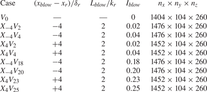
A slot of two-dimensional wall blowing is placed at  $x_{blow}-x_r=\mp 4\delta _r$ for upstream or downstream blowing position cases, and the width of the slot is
 $L_{blow}=2k_r$. The formula for the profile of wall blowing is
 \begin{equation} \rho_w v_w(x)=\frac{I_{blow}}{2}\rho_\infty{u}_\infty\left[\cos\frac{{2}{\rm \pi} (x-x_{blow})}{L_{blow}}+1\right], \end{equation}
where  $v$ is the wall-normal velocity and
 $I_{blow}=(\rho _w v_w)_{max}/\rho _\infty {u}_\infty$ represents the intensity of blowing. For the cases simulated in this paper, different values of
 $I_{blow}$ are employed. Parameters for wall blowing and the grid dimensions of all the cases are reported in table 3 (where
 $n_x\times {n}_y\times {n}_z$ are the number of grid points in the three directions).
Details of all cases in this paper.

The configuration of the computational domain is illustrated in figure 1. The size of the well-resolved region in the computational domain is  $L_x\times {L}_y\times {L}_z=150\delta _r\times 28.6\delta _r\times 10\delta _r$. The inlet boundary is placed at
 $x_{in}-x_r=-50\delta _r$. At the end of the domain, there is a sponge region where the grid is gradually coarsened in the streamwise direction in order to dissipate spurious wave reflections generated at the outlet boundary. The length of the sponge region is
 $x_{sponge}=50\delta _r$.
Computational domain configuration.

Values of  $L_y$ and
 $L_z$ are referenced to Pirozzoli et al. (Reference Pirozzoli, Grasso and Gatski2004). To verify whether the width of domain
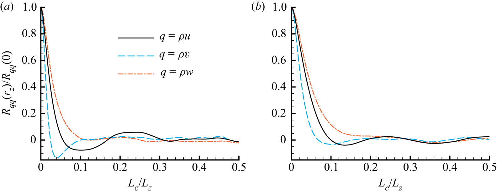
 $L_z$ is large enough, correlation coefficients in the spanwise direction are analysed. The correlation for quantity
 $q$ is defined as (Pirozzoli et al. Reference Pirozzoli, Grasso and Gatski2004)
 \begin{equation} R_{qq}(L_c)=\sum^{n_z-1}_{k=1} \overline{q^{\prime}_k q^{\prime}_{k+k_c}}, \end{equation}
where  $\bar {q}$ is the Reynolds average of quantity
 $q$,
 $q^{\prime }=q-\bar {q}$ represents the fluctuations and
 $L_c=k_cL_z/n_z$ is the distance between two points. The spanwise correlation coefficients at two different positions are shown in figure 2. It is clear that coefficients for the three components of the momentum vector at these two positions reduce rapidly within
 $L_c<0.1L_z$ and approach zero beyond that distance.
Spanwise correlation coefficients at  $x-x_r=95\delta _r$ and (a)
 $y=k_r$ or (b)
 $y=\delta _r$.

At the inlet boundary, a compressible laminar boundary layer profile also obtained by solving (2.1) is imposed. A comparison is presented in figure 3 between two-dimensional DNS results and solutions of compressible Blasius equations with the similarity transformation to validate the inlet boundary profile. As is apparent, the similarity solution is in exceptional agreement with the DNS result. For the two lateral boundaries of the domain, the periodic condition is employed, and the non-slip isothermal wall condition is adopted for the wall boundary along with the boundary layer equation  $\partial {p}/\partial \boldsymbol {n}=0$ (here
 $p$ is the static pressure and
 $\boldsymbol {n}$ denotes the wall-normal vector). In addition, a non-reflecting boundary condition (Poinsot & Lele Reference Poinsot and Lele1992; Pirozzoli, Grasso & D'Andrea Reference Pirozzoli, Grasso and D'Andrea2001) is used for the upper boundary, and a pressure outlet condition (Pirozzoli et al. Reference Pirozzoli, Grasso and Gatski2004) is employed for the outlet boundary.
Validation of similarity solution used as the inlet boundary profile: (a) streamwise velocity  $u$ and (b) temperature
 $T$.

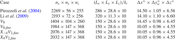
The grid resolution for all the cases is  ${\rm \Delta} {x}^+\times {\rm \Delta} {y}^+_w\times {\rm \Delta} {z}^+=14.45\times 0.98\times 6.45$ (dimensionless grid size is defined as
 ${\rm \Delta} {x}^+_i=\sqrt {\tau _w\rho _w}{\rm \Delta} {x}_i/\mu _w$, where
 $\tau _w$ is the wall shear stress and
 ${\rm \Delta} {x}_i$ represents the grid size in direction
 $i$), which is basically the same as in Pirozzoli et al. (Reference Pirozzoli, Grasso and Gatski2004) (see table 4). In regions over the roughness element or the blowing slot, the grid is refined to provide a better description. The distributions of grid points in the near region of the roughness and slot are demonstrated in figure 4.
Grid point distributions on (a) wall boundary and (b) axial plane (displaying every second grid point in each direction).

Grid resolution and sensitivity study.

A grid sensitivity study is also conducted to verify the grid dimension, and the reference cases are reported in table 4. For the cases with subscript  $fine$, the mesh is refined in all three directions based on the original cases. A comparison of Reynolds- and spanwise-averaged skin friction distributions between case
 $V_0$ and case
 $X_4V_2$ is plotted in figure 5(a). The skin friction formula given by White & Christoph (Reference White and Christoph1972) is employed as a reference:
 \begin{align} C_f=\frac{0.455}{S^2}\ln^{{-}2}\left(\frac{0.06xRe_{ref}}{S\bar{\mu}_w/\mu_\infty} \sqrt{\frac{T_\infty}{T_w}}\right), \quad S=\frac{\sqrt{T_w/T_\infty-1}}{\arcsin{A}},\quad A=\sqrt{\frac{(\gamma-1){Ma}^2_\infty}{2T_w/T_\infty}}. \end{align}
The results show a good agreement between the two cases. Moreover, the skin friction coefficients of both cases in the fully developed turbulence region correspond well to the theoretical estimate formula.
Grid sensitivity study and result validation: skin friction distributions of (a) case  $V_0$, (c) case
 $X_{-4}V_2$ and (d) case
 $X_4V_2$, and (b) van Driest velocity profiles at
 $x-x_r=95\delta _r$ of case
 $V_0$.

In figure 5(b), the Reynolds- and spanwise-averaged van Driest velocity  $U_{VD}^+$ (van Driest Reference van Driest1951) profiles of both cases at
 $x-x_r=95\delta _r$ are compared with results from Li et al. (Reference Li, Fu, Ma and Gao2009), where
 \begin{equation} y^+{=}\frac{\rho_w u_\tau{y}}{\mu_w},\quad U_{VD}^+{=}\frac{U_{VD}}{u_\tau},\quad u_\tau=\sqrt{\frac{\tau_w}{\rho_w}},\quad U_{VD}=\int^u_0\sqrt{\frac{\rho}{\rho_w}}\,\textrm{d}u. \end{equation}
In addition, the theoretical formulae – the viscous sublayer linear solution  $U_{VD}^+=y^+$ and the logarithmic layer solution
 $U_{VD}^+=2.5\ln {y^+}+5.5$ (Coles Reference Coles1956) – are also given for reference purposes. As can be seen, the results for case
 $V_0$ agree well with all the reference values in both the inner layer and the log layer. The discrepancy in the wake layer is mainly because the position where we obtain the profile differs from that in Li et al. (Reference Li, Fu, Ma and Gao2009), and as a result the boundary layer thickness is different. The results in figure 5 indicate that the grid resolution is fine enough to deliver a good accuracy for DNS of roughness-induced transition.
Besides, the skin frictions of case  $X_{-4}V_2$ and case
 $X_4V_2$ are also compared with their corresponding reference cases, respectively (see figures 5a and 5b). The results show that the mesh employed in our study can also describe the influence of wall blowing well enough.
In this paper, the unsteady compressible Navier–Stokes equations are employed as the governing equations:
 \begin{equation} \frac{\partial\boldsymbol{Q}}{\partial{t}} +\frac{\partial\boldsymbol{F}_{c,j}}{\partial{x_j}}= \frac{\partial\boldsymbol{F}_{v,j}}{\partial{x_j}} \quad (\,j=1,2,3), \end{equation}
where  $\boldsymbol {Q}$ is the vector of conservative variables, and
 $\boldsymbol {F}_{c,j}$ and
 $\boldsymbol {F}_{v,j}$ represent convective and viscous flux vectors in three directions, respectively. They can be calculated as
 \begin{align}
\left.\begin{array}{c@{}} \boldsymbol{Q}=\begin{pmatrix} \rho
\\ \rho{u_i} \\ \rho{e} \end{pmatrix},\quad
\boldsymbol{F}_{c,j}=\begin{pmatrix} \rho{u_j} \\ \rho{u}_i
u_j+p\delta_{ij} \\ (\rho{e}+p)u_j \end{pmatrix},\quad
\boldsymbol{F}_{v,j}=\begin{pmatrix} 0 \\ \sigma_{ij} \\
\sigma_{ij}u_i+q_j \end{pmatrix}, \quad (i,j=1,2,3),\\
\displaystyle
e=\dfrac{p}{(\gamma-1)\rho}+\dfrac{u_i^2}{2},\quad
\sigma_{ij}= \left\{ \begin{array}{@{}l} \displaystyle
\mu\left(\dfrac{\partial{u}_j}{\partial{x}_i}
+\dfrac{\partial{u}_i}{\partial{x}_j}\right), \quad i\ne{j},\\ \displaystyle
2\mu\dfrac{\partial{u}_i}{\partial{x}_i}
-\dfrac{2}{3}\mu\boldsymbol{\nabla}\boldsymbol{\cdot}\boldsymbol{u}, \quad i=j, \end{array} \right.
\quad q_i=k\frac{\partial{T}}{\partial{x}_j},
\end{array}\right\}
\end{align}
where  $\delta _{ij}$ is the Kronecker delta,
 $\boldsymbol {u}$ represents the velocity vector and
 $k$ is the thermal conductivity.
To solve the body-fitted mesh that describes the shape of the smooth-edged roughness element, governing equations in curvilinear coordinates (Deng et al. Reference Deng, Mao, Tu, Liu and Zhang2011) are employed. In this paper, the governing equation is solved with the finite-difference code OpenCFD developed by Li et al. (Reference Li, Fu, Ma and Liang2010). The parallel code has been proven to be reliable in multiple studies (Li et al. Reference Li, Fu, Ma and Gao2009; Lu et al. Reference Lu, Liu, Liu and Yan2020a,Reference Lu, Liu, Liu and Yanb). For the spatial discretization of the convective terms, the WENO-SYMBO method (Martin et al. Reference Martin, Taylor, Wu and Weirs2006) with Steger–Warming splitting (Steger & Warming Reference Steger and Warming1981) is used. The viscous terms are computed with an eighth-order central-differencing scheme. A third-order total variation diminishing type Runge–Kutta method (Jiang & Shu Reference Jiang and Shu1996) is applied for time advancing.
3. Results
First, the relative friction drag for the baseline case  $V_0$ and cases with weak wall blowing (
 $I_{blow}\le 0.04$) are demonstrated in table 5. It can be seen that both upstream and downstream-positioned blowing show a significant effect of reducing skin friction. In addition, the effect is remarkably enhanced with the increase in
 $I_{blow}$.
Relative friction drag (the result of case  $V_0$ is set to
 $1.00$).

To further explore the role of wall blowing in the reduction of skin friction, a Fukagata–Iwamoto–Kasagi (FIK) decomposition (Fukagata, Iwamoto & Kasagi Reference Fukagata, Iwamoto and Kasagi2002) is conducted for these cases. For the plane compressible boundary layer with a zero pressure gradient, the skin friction can be decomposed into five components: laminar, turbulent, compressible, compressible–turbulent interaction and spatial development contributions (Gomez, Flutet & Sagaut Reference Gomez, Flutet and Sagaut2009). The formula can be written as
 \begin{equation} C_f=\underbrace{\frac{4}{Re_\delta}\int^1_0\overline{\rho_*u_*}\,\textrm{d} y_*}_{C_{f,L}}+ \underbrace{4\int^1_0(1-y_*) \overline{\rho_*u_*^{\prime\prime}v_*^{\prime\prime}}\,\textrm{d} y_*}_{C_{f,T}}+\,C_{f,{C}}+C_{f,{CT}}+C_{f,{D}}, \end{equation}
where the boundary layer thickness Reynolds number  $Re_\delta =\rho _\infty {u}_\infty \delta /\mu _w$ (with
 $\delta$ the local boundary layer thickness),
 $q_*$ represents the non-dimensional value of quantity
 $q$ based on
 $\rho _\infty$,
 $u_\infty$,
 $T_w$ and
 $\delta$, and
 $q^{\prime \prime }$ is the fluctuation value of quantity
 $q$ based on Favre averaging.
For cases in this study,  $C_{f,L}$ and
 $C_{f,T}$ are the two main components of
 $C_f$, so their results are reported in figures 6 and 7. As shown in figure 6, the gap between the distributions of
 $C_{f,L}$ in these cases is small. Therefore, the main contribution to the reduction of the friction drag force should be the turbulent contribution
 $C_{f,T}$.
Spanwise-averaged  $C_{f,x}$ and
 $C_{f,L}$ distributions of case
 $V_0$ and cases with blowing in (a) upstream position and (b) downstream position.

The  $C_{f,T}$ distributions of (a) case
 $V_0$, (b) case
 $X_{-4}V_2$, (c) case
 $X_{-4}V_4$, (d) case
 $X_4V_2$ and (e) case
 $X_4V_4$. (The dashed line indicates the roughness shape at the height of
 $k_r/2$.)

The presumption above can be confirmed with the distributions of  $C_{f,T}$ drawn in figure 7. In case
 $V_0$, behind the roughness element, a wake region is formed where the velocity fluctuation grows much more rapidly than in other regions. Then, it develops into a turbulent wedge downstream and continuously broadens in the spanwise direction. Figure 7(b–e) shows that both upstream- and downstream-positioned blowing are able to significantly inhibit the transition process. For both cases in which
 $I_{blow}=0.02$, the formation of a turbulent wedge is largely delayed. Moreover, the transition induced by the roughness element entirely disappears when the value of
 $I_{blow}$ continues to increase. In conclusion, both upstream- and downstream-positioned blowing is able to reduce skin friction by inhibiting the roughness-induced transition.
In order to investigate the role of wall blowing in transition delay, it is necessary to clarify the mechanism of transition induced by smooth-edged roughness element in case  $V_0$.
3.1. Smooth-edged roughness-induced transition
According to Subbareddy et al. (Reference Subbareddy, Bartkowicz and Candler2014), typical structures in high-speed flow past a roughness element consist of (1) a horseshoe vortex system formed in the upstream separation zone, (2) an upstream shockwave system and (3) a separated shear layer/counter-rotating vortex system. These structures in case  $V_0$ are visualized in figure 8. The
 $Q$ criterion in this figure is the second invariant of
 $\boldsymbol {\nabla }\boldsymbol {u}$ (Hunt, Wray & Moin Reference Hunt, Wray and Moin1988):
 \begin{equation} Q={-}\frac{1}{2}\left[\left(\frac{\partial{u}}{\partial{x}}\right)^2+ \left(\frac{\partial{v}}{\partial{y}}\right)^2+\left(\frac{\partial{w}}{\partial{z}} \right)^2\right]-\frac{\partial{u}}{\partial{y}}\frac{\partial{v}}{\partial{x}}- \frac{\partial{u}}{\partial{z}}\frac{\partial{w}}{\partial{x}}- \frac{\partial{v}}{\partial{z}}\frac{\partial{w}}{\partial{y}}. \end{equation}
Visualization of the flow field, consisting of streamlines passing through the line  $(x-x_r=-50\delta _r,\ y=0.1\delta _r)$ (dark grey) or the line
 $(x-x_r=-50\delta _r,\ y=0.2\delta _r)$ (light grey), streamlines on the symmetry plane and a slice
 $x-x_r=10\delta _r$ (black), streamwise skin friction coefficient contour on the wall, non-dimensional pressure contour on the symmetry plane and non-dimensional
 $Q$ criterion contours on slices
 $x-x_r=7\delta _r$ and
 $x-x_r=10\delta _r$ (here
 $p_{ref}=\gamma {Ma}_\infty ^2$ and
 $Q_{ref}=u_\infty ^2/\delta _r^2$).

To determine which structure is the main source of unsteadiness in the transition process, five probes are adopted in the flow field (see figure 8) to record the fluctuation of pressure. Probes 1 and 2 are placed in the upstream separation zone, probe 3 is located at the shockwave, and probes 4 and 5 are in the counter-rotating vortex structure at  $x-x_r=7\delta _r$ or
 $x-x_r=10\delta _r$. The power spectral density (PSD) of the pressure fluctuations at these probes is drawn in figure 9. The PSD spectrum is estimated using a fast Fourier transform (FFT) with uniform window. The sampling frequency is
 ${St}_{{PSD}}=192.31$ (where
 $St$ is the Strouhal number based on
 $\delta _r$ and
 $u_\infty$), and
 $10\ 000$ steps are recorded for each probe. The results show that the pressure fluctuations at the upstream separation region and the shockwave have the same dominant frequency (named mode 2). However, mode 2 disappears in the downstream region. At probes 4 and 5, the features of the dominant mode (named mode 1) are totally different from those of mode 2. The frequency of mode 1 is
 ${St}_1=0.422$ and that of mode 2 is
 ${St}_2=4.21$. The Strouhal number of mode 1 based on
 $u_k$ and
 $\delta ^*_r$ (displacement thickness at
 $x_r$) is
 ${St}_{k,1}=0.309$, which is in the frequency range
 $0.2\le {St}_k\le 0.5$ given by Klebanoff, Cleveland & Tidstrom (Reference Klebanoff, Cleveland and Tidstrom1992). Moreover, the frequency range of mode 1 is much wider than that of mode 2 in the spectrum. Recent studies of roughness-induced transition in the incompressible regime have shown that the dominant unsteadiness in the flow field results from the distorted wake structure downstream of the roughness (Loiseau et al. Reference Loiseau, Robinet, Cherubini and Leriche2014; Citro et al. Reference Citro, Giannetti, Luchini and Auteri2015; Bucci et al. Reference Bucci, Puckert, Andriano, Loiseau, Cherubini, Robinet and Rist2018; Puckert & Rist Reference Puckert and Rist2018, Reference Puckert and Rist2019). Therefore, we can assume that the unsteadiness in the roughness-induced transition process of case
 $V_0$ mainly comes from the separated shear layer/counter-rotating vortex system in the downstream region of roughness.
PSD results of pressure fluctuations at (a) probes 1–3 and (b) probes 4–5 (here  $S_{ref}=p_{ref}^2\delta _r/u_\infty$).

To confirm the assumption, we perform a flow freezing operation (Shrestha & Candler Reference Shrestha and Candler2019). In this operation, the conservative variables  $\boldsymbol {Q}$ in the freezing zone are fixed at average value. Flow in the upstream region of the roughness element is frozen so that the upstream separation zone and the shockwave can contribute little to the unsteadiness in the downstream region. However, it can be observed from figure 10 that the freezing of the upstream flow rarely affects the development of disturbance. This proves that the main unsteadiness in the roughness-induced transition process originates from the downstream region.
Comparison of non-dimensional velocity fluctuation distributions on the plane  $y=k_r$ between (a) case
 $V_0$ and (b) case
 $V_0$ with a flow freezing operation. (The dashed line indicates the roughness shape at the height of
 $k_r/2$.)

Additionally, three-dimensional spectral proper orthogonal decomposition (SPOD) (Lumley Reference Lumley1970) and DMD (Rowley et al. Reference Rowley, Mezić, Bagheri and Schlatter2009; Schmid Reference Schmid2010) of the near-roughness region ( $-2.75\delta _r\le {x}-x_r\le 12.75\delta _r$,
 $y\le 1.25\delta _r$ and
 $-2.5\delta _r\le {z}\le 2.5\delta _r$) are conducted to support the findings above. The total number of grid points is approximately 1.5 million, and
 $500$ snapshots are recorded for our study. The sampling frequency is
 ${St}_{{SPOD}}={St}_{{DMD}}=38.46$. For SPOD, the number of snapshots in each block is
 $N_f=250$, and the number of overlap snapshots is
 $N_o=225$. An identity matrix is used as the weight matrix. The code we use for SPOD is provided by Towne, Schmidt & Colonius (Reference Towne, Schmidt and Colonius2018). The SPOD results are consistent with the PSD analysis above. The peak of mode 2 appears clearly in the SPOD spectra for the upstream region of roughness (
 $x-x_r\le -0.85\delta _r$) (see figure 11a), and almost disappears in the results of the whole near-roughness region (see figure 11b). The dominant mode in the spectra of near-roughness region is mode 1.
SPOD results of (a) the upstream region ( $-2.75\delta _r\le {x}-x_r\le -0.85\delta _r$,
 $y\le 1.25\delta _r$ and
 $-2.5\delta _r\le {z}\le 2.5\delta _r$) and (b) the whole near-roughness region (
 $-2.75\delta _r\le {x}-x_r\le 12.75\delta _r$,
 $y\le 1.25\delta _r$ and
 $-2.5\delta _r\le {z}\le 2.5\delta _r$) of case
 $V_0$. (The grey areas are the
 $99\,\%$ confidence interval.)

The algorithm for DMD employed in this paper comes from Sayadi & Schmid (Reference Sayadi and Schmid2016), and sparsity-promoting DMD (DMDSP) (Jovanović, Schmid & Nichols Reference Jovanović, Schmid and Nichols2014) is also used here to select the dominant DMD modes. From the distribution of eigenvalues shown in figure 12(a), we can see that most of the modes are on the unit circle, which indicates that the development of the flow field is saturated (Subbareddy et al. Reference Subbareddy, Bartkowicz and Candler2014). Both the upstream and downstream dominant modes can be picked out by DMDSP with different parameters, and the results reveal that mode 1 is much more dominant than mode 2. Figure 12(b) demonstrates the pressure fluctuation of mode 1 extracted by DMD analysis, and figure 12(c) is the distribution of the shear layer separated from the roughness element. The shear layer is indicated by local shear  $u_s$ (Shrestha & Candler Reference Shrestha and Candler2019):
 \begin{equation} u_s=\sqrt{\left(\frac{\partial{u}}{\partial{y}}\right)^2+ \left(\frac{\partial{u}}{\partial{z}}\right)^2}. \end{equation}
The fluctuation growth of unstable mode 1 is mainly in the downstream region of the roughness, and the position where the amplitude of fluctuation increases most rapidly is close to the shear layer. This is consistent with our supposition above that the main source of unsteadiness in the transition process is the separated shear layer/counter-rotating vortex system in the wake structure. Besides, the pressure fluctuations of mode 1 at  $x-x_r=11.5\delta _r$ and
 $x-x_r=12.5\delta _r$ show axial symmetry, and the maximum value of fluctuation is situated along the symmetry axis (see figure 12d,e). This agrees with the feature of a varicose mode, which exists due to the instability of the shear layer induced by the counter-rotating vortex pair in the wake (De Tullio et al. Reference De Tullio, Paredes, Sandham and Theofilis2013).
DMD results of case  $V_0$: (a) eigenvalues from standard DMD and DMDSP with
 $N_z$ DMD modes; (b) reconstruction of mode 1 extracted by DMD; (c) the distribution of streamwise shear on the symmetry plane (
 $u_{s,ref}=u_\infty /\delta _r$); and reconstruction of mode 1 at (d)
 $x-x_r=11.5\delta _r$ and (e)
 $x-x_r=12.5\delta _r$. (The grey solid lines in panels (d,e) are isolines of
 $u$ with the same value set, and the black dashed line indicates the projection of roughness.)

To further demonstrate the relationship between the separated shear layer/counter- rotating vortex system and the development of disturbances, several slices of the flow field for case  $V_0$ are drawn in figure 13. In figure 13(a) we can clearly observe that the horseshoe vortex and the counter-rotating vortex pair trail downstream behind the roughness, and the separated shear layer forms over the counter-rotating vortex. The in-plane streamlines illustrate a heavy distortion of the boundary layer caused by the streamwise vortices in the wake structure. With the flow going downstream, all the streamwise vortices in the wake are dissipated, and the distortion is relaxed. However, the separated shear layer is bent by the counter-rotating vortex pair and gradually wraps around it. The interaction of the separated shear layer/counter-rotating vortex system maintains the strength of the shear layer and induces a rapid disturbance growth at its position (see figure 13b,d, f). In addition, the lift-up effect (Landahl Reference Landahl1980; Brandt Reference Brandt2014) caused by the streamwise counter-rotating vortex not only induces disturbance transient growth (Reshotko Reference Reshotko2001) but more importantly amplifies the interaction, which is also observed by Shrestha & Candler (Reference Shrestha and Candler2019).
Slices of case  $V_0$ at (a,b)
 $x-x_r=6\delta _r$, (c,d)
 $x-x_r=10\delta _r$ and (e, f)
 $x-x_r=14\delta _r$ coloured with (a,c,e) non-dimensional
 $Q$ criterion and (b,d, f) streamwise velocity fluctuation. (The dark grey solid lines on the left half of (a,c,e) are isolines of
 $u_s$ with the same value set; the light grey lines on the right are in-plane vortex lines; and the black dashed line indicates the projection of roughness.)

3.2. Weak wall blowing inhibiting transition
With the understanding of the smooth-edged roughness-induced transition in § 3.1, we can now look into the mechanism of two-dimensional upstream-/downstream-positioned weak wall blowing inhibiting transition.
For the two cases with upstream-positioned weak blowing  $X_{-4}V_2$ and
 $X_{-4}V_4$, the same three slices of the flow field are plotted in figure 14 as a comparison with case
 $V_0$. It is obvious that the configuration of the wake structure changes little at
 $x-x_r=6\delta _r$ between cases with or without upstream-positioned blowing. Only the strength of those main structures in the wake is diminished and the distortion of the boundary layer profile is reduced. As a result, the interaction between the separated shear layer and counter-rotating vortex is inhibited, and the shear layer is not as bent as in case
 $V_0$ and is also relaxed along the streamwise direction, especially in case
 $X_{-4}V_4$. Therefore, the disturbance growth rate is decreased. As roughness-induced transition is a competitive mechanism between the development of unsteady fluctuation and the relaxation of the wake structure (Ergin & White Reference Ergin and White2006), the transition process in both cases with upstream blowing position is delayed, as shown in figure 7.
Slices of (a,c,e) case  $X_{-4}V_2$ and (b,d, f) case
 $X_{-4}V_4$ at (a,b)
 $x-x_r=6\delta _r$, (c, d)
 $x-x_r=10\delta _r$ and (e, f)
 $x-x_r=14\delta _r$ coloured with the non-dimensional
 $Q$ criterion. (The dark grey solid lines on the left half are isolines of
 $u_s$ with the same value set; the light grey lines on the right are in-plane vortex lines; and the black dashed line indicates the projection of roughness.)

It is actually easy to understand the mechanism of the wake structure being weakened by upstream-positioned blowing. The upstream-positioned blowing does not directly interact with the wake structure. Instead, the comparison of the boundary layer profile on the symmetry plane between cases  $V_0$ and
 $X_{-4}V_4$ drawn in figure 15 shows that the upstream-positioned blowing is able to lift the inflow boundary layer, which may result in a decrease in the effective value of
 $Re_{kk}$. Therefore, we conduct two-dimensional DNS computations of upstream-positioned weak wall blowing cases but without the roughness element, and the results are reported in table 6. From the results we can see that the upstream-positioned blowing greatly reduces the effective roughness Reynolds number
 $Re_{kk}^*$, which leads to the weakening of the wake structure. In addition, the zoomed-in boundary layer profile demonstrates that the upstream-positioned blowing also has the effect of moving the separation position backwards, which determines the structures of the horseshoe vortex system forming in the separation zone (Baker Reference Baker1979).
Profiles of non-dimensional streamwise velocity on the symmetry plane of (a,c) case  $V_0$ and (b,d) case
 $X_{-4}V_4$. Panels (c,d) are zoomed-in views of the grey dashed rectangular regions in panels (a,b); black solid lines are in-plane streamlines.

Effective roughness Reynolds number and inflow boundary layer parameters (here  $\delta _r^*$ is the actual boundary layer thickness at the centre point of roughness).

The PSD results illustrated in figure 16 for both cases with upstream blowing position also support our analysis. Owing to the changes in vortex structures in the upstream separation zone shown in figure 15, the unstable mode 2 in the upstream region is weakened in case  $X_{-4}V_2$ and disappears in case
 $X_{-4}V_4$. In the downstream region, the unstable mode 1 has the same varying tendency. The amplitudes of both modes are reduced by approximately an order of magnitude in case
 $X_{-4}V_2$ compared with case
 $V_0$. Additionally, the frequency of mode 1 falls with the reduction of
 $Re_{kk}^*$, which agrees with the result reported by Klebanoff et al. (Reference Klebanoff, Cleveland and Tidstrom1992).
PSD results of (a,c) case  $X_{-4}V_2$ and (b,d) case
 $X_{-4}V_4$ at the (a,b) upstream region and (c,d) downstream region.

In regard to downstream blowing position, its effect is the delay of the roughness-induced transition through completely different mechanisms. The comparison between figures 17 and 15(c) shows that the downstream-positioned blowing has much less impact on the separation zone and horseshoe vortex system than the upstream-positioned blowing. This suggests that the contribution of downstream-positioned blowing in delaying the transition mainly comes from its direct interaction with the downstream wake structure.
Profiles of the non-dimensional streamwise velocity on the symmetry plane of (a) case  $X_4V_2$ and (b) case
 $X_4V_4$. (Black solid lines are in-plane streamlines.)

The slices of case  $X_4V_2$ at
 $x-x_r=5\delta _r$ demonstrated in figure 18(b) indicate that the wake structure in the downstream region of cases with downstream blowing position is distinct from cases with upstream blowing position or without blowing, which is apparently due to the direct interaction between the wake structure and wall blowing. The main difference is that a new vortex pair is formed under the original counter-rotating vortex pair in case
 $X_4V_2$, and the rotation directions of these two vortex pairs are opposite. The original counter-rotating vortex pair is squeezed and pushed away from the wall in the wall-normal direction and stretched in the spanwise direction. The new vortex pair comes from the secondary vortex induced by the original counter-rotating vortex pair in the near-wall region due to the no-slip wall boundary condition. As illustrated in figure 18(d), the secondary vortex is lifted away from the wall by downstream-positioned wall blowing.
Comparison of wake structures between (a,c) case  $V_0$ and (b,d) case
 $X_4V_2$: (a,b) slices of the non-dimensional
 $Q$ criterion at
 $x-x_r=5\delta _r$ and (c,d) non-dimensional streamwise angular velocity profiles at
 $z=0.3\delta _r$. (The grey solid lines are in-plane streamlines, and the black dashed line indicates the projection of roughness,
 $\omega _{ref}=u_\infty /\delta _r$.)

For a further exploration of wake structure development in cases with downstream blowing position, the same three slices of the boundary layer are drawn in figure 19. The results suggest that the weakening of the separated shear layer caused by the downstream-positioned blowing is not as effective as that due to upstream-positioned blowing with the same intensity. However, the downstream-positioned blowing is able to provide a similar effect to the upstream-positioned blowing on diminishing the magnitude of the counter-rotating vortex pair in the wake. Therefore, the shear layer/counter-rotating vortex interaction is weakened, and the shear layer is less bent than in case  $V_0$. As a result, the disturbance development induced by the interaction is inhibited and the transition is delayed as displayed in figure 7. In summary, the downstream-positioned blowing takes effect on delaying the roughness-induced transition by rapidly diminishing the magnitude of the counter-rotating vortex pair in the wake structure.
Slices of (a,c,e) case  $X_4V_2$ and (b,d, f) case
 $X_4V_4$ at (a,b)
 $x-x_r=6\delta _r$, (c,d)
 $x-x_r=10\delta _r$ and (e, f)
 $x-x_r=14\delta _r$ coloured with the non-dimensional
 $Q$ criterion. (The dark grey solid lines on the left half are isolines of
 $u_s$ with the same value set; the light grey lines on the right are in-plane vortex lines; and the black dashed line indicates the projection of roughness.)

Two possible approaches are proposed here to explain the weakening of the counter-rotating vortex pair: the downstream-positioned blowing can provide much stronger dissipation for streamwise vortices, and the two-dimensional wall blowing is able to convert some streamwise vorticities into spanwise types. To confirm our supposition, vorticity transportation analysis is employed. For quantity  $\omega ^2_i/2$ (where
 $\omega _i$ represents the angular velocity component in direction
 $i$), its transportation equation can be written as (Brown, Lee & Moser Reference Brown, Lee and Moser2015; Suryanarayanan et al. Reference Suryanarayanan, Goldstein, Berger, White and Brown2020):
 \begin{equation} \frac{\partial}{\partial{t}} (\frac{1}{2}\omega_i^2 )+ \boldsymbol{u}\boldsymbol{\cdot}\boldsymbol{\nabla} (\frac{1}{2}\omega_i^2 )= \omega_i\boldsymbol{\omega}\boldsymbol{\cdot}\boldsymbol{\nabla}{u}_i+ \nu[\nabla^2 (\frac{1}{2}\omega_i^2)-|\boldsymbol{\nabla}\omega_i|^2], \end{equation}
where  $\boldsymbol {\omega }$ is the angular velocity vector. In this equation, the dissipation term is
 $D_i=\nu |\boldsymbol {\nabla }\omega _i|^2$, and the source term is
 $S_i=\omega _i\,\boldsymbol {\omega }\boldsymbol {\cdot }\boldsymbol {\nabla }{u}_i=\sum _jS_{ij}$. The component of the source term
 $S_{ii}=\omega _i^2\,\partial {u_i}/\partial {x_i}$ represents the stretch of
 $\omega _i$, and component
 $S_{ij}=\omega _i\omega _j\,\partial {u_i}/\partial {x_j}$ denotes the conversion from
 $\omega _j$ to
 $\omega _i$.
Profiles of the vortex transportation are plotted in figure 20 to verify the first approach. It can be observed in figure 20(b) that the counter-rotating vortex experiences a short period of increase upstream of the blowing slot. This results from the stretch of  $\omega _x$ induced by wall blowing (see the peak value of
 $S_{xx}$ in figure 20d). Meanwhile, as demonstrated in figure 18(d), the wall blowing can also lift the counter-rotating vortex pair and its secondary vortex and squeeze the space between them. Both enlarging the magnitude of the streamwise vortex and squeezing them in the wall-normal direction are able to increase the gradient of
 $\omega _x$ and consequently provide a much stronger dissipation than in case
 $V_0$ (see figure 20e, f).
Profiles of (a,c,e) case  $V_0$ and (b,d, f) case
 $X_4V_4$ at
 $z=0.5\delta _r$ coloured with (a,b) the non-dimensional streamwise angular velocity, (c,d) vorticity transportation term
 $S_{xx}$ and (e, f)
 $D_x$.

Similarly, the second approach can be proven by comparing the profiles of source term  $S_{zx}$ drawn in figure 21. In figure 21(b), an obvious peak region can be observed over the blowing slot located at
 $x_{blow}-x_r=4\delta _r$. The peak value of
 $S_{zx}$ indicates a strong conversion from the streamwise vorticity to the spanwise type, which also contributes to the weakening of the counter-rotating vortex pair.
Profiles of (a) case  $V_0$ and (b) case
 $X_4V_4$ at
 $z=0.5\delta _r$ coloured with the non-dimensional vorticity transportation term
 $S_{zx}$.

PSD analyses are also conducted for these two cases with downstream-positioned weak wall blowing, and their results shown in figure 22 agree well with our analysis above. As the downstream-positioned blowing has little influence on the upstream region, which is shown in figure 17, the unstable mode 2 always exists, even in case  $X_4V_4$, where the transition does not occur downstream. However, for the downstream region, the dominant mode 1 only exists in case
 $X_4V_2$, and its amplitude is decreased compared to case
 $V_0$. Moreover, as the effect of downstream-positioned blowing on reducing
 $Re_{kk}^*$ is not as great as the upstream one, the frequency of mode 1 in case
 $X_4V_2$ is between case
 $V_0$ and case
 $X_{-4}V_2$.
PSD results of (a,c) case  $X_4V_2$ and (b,d) case
 $X_4V_4$ at the (a,b) upstream region and (c,d) downstream region.

3.3. Strong wall blowing promoting transition
According to the results demonstrated in table 5, the skin friction decreases with increasing  $I_{blow}$ for both upstream- and downstream-positioned weak wall blowing. However, this trend cannot always continue. The results reported in table 7 indicate that, in cases with strong wall blowing, the increase in
 $I_{blow}$ leads to a significant growth in the friction drag force.
Relative friction drag (the result of case  $V_0$ is set to
 $1.00$).

Experimental (Bajura & Catalano Reference Bajura and Catalano1975), theoretical (Tsuji et al. Reference Tsuji, Morikawa, Nagatani and Sakou1977) and numerical (Wernz & Fasel Reference Wernz and Fasel1997) studies have shown that two-dimensional wall blowing with overstrength can introduce unsteadiness into the flow field and lead to transitions downstream. Similar results are also observed in this study. From figure 23, we can see that, in contrast to weak wall blowing cases, flow in the wake remains laminar when  $I_{blow}$ is small (cases
 $X_{-4}V_{18}$ and
 $X_4V_{23}$), and breaks down into turbulence in cases with stronger blowing (cases
 $X_{-4}V_{20}$ and
 $X_4V_{25}$).
The  $C_{f,T}$ distributions of (a) case
 $X_{-4}V_{18}$, (b) case
 $X_{-4}V_{20}$, (c) case
 $X_4V_{23}$ and (d) case
 $X_4V_{25}$. (The dashed line indicates the roughness shape at the height of
 $k_r/2$.)

For the two cases with upstream-positioned strong wall blowing, slices at  $x-x_r=6$ are drawn in figure 24. It can be observed that the separated shear layer in both cases is very weak compared to other cases in this paper, and this can be attributed to the much smaller effective roughness Reynolds number. The value of
 $Re_{kk}^*$ for case
 $X_{-4}V_{18}$ is
 $113.57$, and for case
 $X_{-4}V_{20}$ is
 $72.11$. However, with the value of
 $I_{blow}$ increasing from
 $0.18$ to
 $0.20$, the wake structure experiences a substantial change. The in-plane streamlines in figure 24(a) illustrate that the difference of wake structures between case
 $X_{-4}V_{18}$ and case
 $V_0$ is small, but the streamwise vortices in the boundary layer of case
 $X_{-4}V_{20}$ become stronger and form much more complicated flow structures. This is because the wake in case
 $X_{-4}V_{20}$ soon becomes unstable and induces a much stronger disturbance than that in
 $X_{-4}V_{18}$ (see figure 24d).
Slices of (a,c) case  $X_{-4}V_{18}$ or (b,d) case
 $X_{-4}V_{20}$ at
 $x-x_r=6\delta _r$ coloured with (a,b) the non-dimensional
 $Q$ criterion and (c,d) the streamwise velocity fluctuation. (The dark grey solid lines on the left half of (a,b) are isolines of
 $u_s$ with the same value set; the light grey lines on the right are in-plane streamlines; and the black dashed line indicates the projection of roughness.)

For exploring the source of unsteadiness, the time sequence of pressure fluctuation  $p^{\prime }$ at the upstream region (probes 1 and 2) and
 $x-x_r=6\delta _r$ (probe 6 in figure 24) are recorded for PSD analysis. Owing to the upstream-positioned strong blowing, there exists a strong unstable mode 2 in the upstream separation zone (see figure 25a). (The peak of the PSD spectrum at
 $St\approx 15$ is a harmonic of mode 2.) However, mode 2 still cannot induce a transition downstream. Meanwhile, a new unstable mode appears in the PSD results of case
 $X_{-4}V_{20}$, and it is marked as mode 3. The amplitude of mode 3 is more than one order of magnitude larger than that of mode 2 in figure 25(b), and its frequency is between those of mode 1 and mode 2. More importantly, unlike mode 2, the unstable mode 3 maintains its amplitude in the propagation towards the downstream region. Meanwhile, there exists the unstable mode 1 downstream, which is the dominant mode in the transition process of cases with weak wall blowing or without it. With the findings above, we suppose that mode 1 in the downstream region of case
 $X_{-4}V_{20}$ is induced by mode 3, or mode 3 is the key factor for the transition process of cases with upstream-positioned strong wall blowing.
PSD results of (a,c) case  $X_{-4}V_{18}$ and (b,d) case
 $X_{-4}V_{20}$ at (a,b) the upstream region and (c,d)
 $x-x_r=6\delta _r$.

To determine the source of unstable mode 3, we re-examine the flow field of these two cases. As demonstrated in
figure 26(a,b), a much larger separation zone forms upstream of the blowing slot, which could be the source of mode 3. Therefore, probes 7 and 8 are placed in this separation zone for PSD analysis, and the results of both cases are demonstrated in figure 26(c,d). The unstable mode 3 can be clearly observed at this separation zone in case  $X_{-4}V_{20}$ as the only dominant frequency, while in case
 $X_{-4}V_{18}$, there is no obvious dominant unstable mode in this region.
Separation zone at the upstream region of the blowing slot in (a,c) case  $X_{-4}V_{18}$ and (b,d)
 $X_{-4}V_{20}$: (a,b) streamwise velocity profiles on the symmetry plane (black lines are in-plane streamlines), and (c,d) PSD results.

Then, a flow freezing operation is conducted for the separation zone upstream of the blowing slot in case  $X_{-4}V_{20}$ to confirm the role of unstable mode 3 in the transition process. From the comparison of velocity fluctuation development at
 $y=k_r$ illustrated in figure 27(a,b), we can see that, due to the freezing operation of the separation zone, the disturbance level near the region of the roughness element is diminished by approximately two orders of magnitude. Although the disturbance still grows in the near-wake region, the lower initial disturbance level results in a peak disturbance level that is not enough for breakdown into turbulence when the distortion of the boundary layer profile is relaxed. The PSD results in figure 27(c,d) also agree with our analysis above. As the separation zone located at the upstream side of the blowing slot is frozen, the unstable mode 3 disappears in the upstream region of the roughness element, and mode 2 becomes the only dominant frequency of the spectrum. As a result, the unstable mode 1 does not appear in the downstream region, and there exists no obvious dominant mode at probe 6. The flow freezing operation proves that mode 3 originates from the separation zone upstream of the blowing slot, and it is the key factor for the transition of cases with upstream-positioned strong blowing.
Flow freezing operation: (a,b) comparison of velocity fluctuation distributions at  $y=k_r$ between (a) case
 $X_{-4}V_{20}$ and (b) case
 $X_{-4}V_{20}$ with the flow freezing operation (the dashed line indicates the roughness shape at the height of
 $k_r/2$); and PSD results for case
 $X_{-4}V_{20}$ with the flow freezing operation at (c) upstream region and (d)
 $x-x_r=6\delta _r$.

To get more features of mode 3, modes 1 and 3 extracted by DMD from case  $X_{-4}V_{20}$ are reconstructed in figure 28. As demonstrated in figure 28(a), the distribution of pressure fluctuation amplitude of mode 1 in case
 $X_{-4}V_{20}$ shows a similar symmetry as in case
 $V_0$. Meanwhile, mode 3 presents significant asymmetry, which means that it may contain the sinuous mode related to the instability of the lateral shear layer (De Tullio et al. Reference De Tullio, Paredes, Sandham and Theofilis2013).
Reconstructions of (a) mode 1 at  $x-x_r=7\delta _r$ and (b) mode 3 at
 $x-x_r=8\delta _r$. (The grey solid lines are isolines of u with the same value set, and the black dashed line indicates the projection of roughness.)

Finally, cases with downstream-positioned strong wall blowing are analysed. Flow structures in the region near the roughness element for cases  $X_4V_{23}$ and
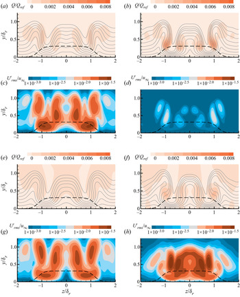
 $X_4V_{25}$ are visualized in figure 29. In both cases, the separation zone upstream of the blowing slot is so large that the roughness element is totally immersed in it, and thus the vortex system in the separation zone is blocked by the roughness element and forms complex structures (see figure 29a,b). For streamwise vortices generated from the roughness element (horseshoe vortex and counter-rotating vortex pair), the effect of stretching provided by downstream-positioned strong wall blowing is much stronger than dissipation (see figure 29e, f). Therefore, streamwise vortices are strengthened with increasing blowing intensity (see figure 29c,d). Moreover, these streamwise vortices in the wake are lifted far away from the wall, and a shear layer subsequently forms under the vortex structures (see figure 29g,h). Similar to case
 $X_{-4}V_{20}$, the flow structure of case
 $X_4V_{25}$ is more complicated than in case
 $X_4V_{23}$ at
 $x-x_r=12\delta _r$ because the wake flow becomes unstable. Figure 29( j) indicates that the velocity fluctuation grows most rapidly at the position of the shear layer in this stage.
Flow visualization of (a,c,e,g,i) case  $X_4V_{23}$ and (b,d, f,h,j) case
 $X_4V_{25}$: (a,b) streamwise velocity profiles at the symmetry plane (black lines are in-plane streamlines), (c,d) profiles of streamwise vorticity at
 $z=-0.9\delta _r$, (e, f) profiles of vorticity transportation
 $(S_x-D_x)/S_{ref}$ at
 $z=-0.9\delta _r$, (g,h) slices of the
 $Q$ criterion at
 $x-x_r=12\delta _r$ (the dark grey solid lines on the left half are isolines of
 $u_s$ with the same value set and the light grey lines on the right are in-plane streamlines), and (i,j) slices of the velocity fluctuation at
 $x-x_r=12\delta _r$ (the black dashed line indicates the projection of roughness).

Following the analyses of other cases above, PSD results for the upstream and downstream regions of both cases are plotted in figure 30. As shown in figure 29, probe 9 is located between the roughness element and the blowing slot, and probe 10 is placed at  $x-x_r=12\delta _r$. The results in figure 30(a,b) suggest that there exists a very low-frequency ingredient, and therefore a much longer signal is adopted for PSD analysis of both cases. It can be observed that there is no dominant unstable mode in the medium- or high-frequency band at the upstream region. Instead, a very low-frequency unstable mode (named mode 4) is obvious at probes 1, 2 and 9 in both cases. In the downstream region, mode 4 maintains its amplitude. In the meantime, mode 1 grows rapidly and becomes the dominant unstable mode at probe 10. Similar to cases with upstream-positioned strong wall blowing, we can assume that the transition occurring in these two cases can be attributed to mode 4.
PSD results of pressure fluctuations for (a,c,e) case  $X_4V_{23}$ and (b,d, f) case
 $X_4V_{25}$ at (a–d) the upstream region of the blowing slot and (e, f)
 $x-x_r=12\delta _r$.

Two different cases with flow freezing operations are simulated to test our assumption. For case  $X_4V_{25}F_1$, the region
 $x-x_r\le -0.777\delta _r$ (upstream region of the roughness element) is frozen, and for case
 $X_4V_{25}F_2$, the freezing region is
 $x-x_r\le 4.287\delta _r$ (blowing slot and the upstream region of it). It can be observed from figure 31(e) that mode 4 still exists with the upstream region of the roughness element being frozen. Meanwhile, in case
 $X_4V_{25}F_2$, the unstable mode 4 totally disappears. This suggests that the very low-frequency mode 4 is generated from the separation zone between the roughness element and the blowing slot. Similar to cases
 $X_4V_{23}$ and
 $X_4V_{25}$, mode 1 is the dominant unstable mode in the downstream region. Owing to the flow freezing operation, the amplitude of mode 1 at probe 10 in case
 $X_4V_{25}F_2$ is even smaller than that in case
 $X_4V_{23}$. However, as demonstrated in figure 31(d), the transition still occurs in the downstream region of case
 $X_4V_{25}F_2$ with only a slight delay due to the lower initial disturbance level downstream of the blowing slot. These results indicate that the very low-frequency mode 4 is not the key factor to determine whether the transition occurs. Instead, it only provides an initial disturbance level for the transition process downstream. The main source of unsteadiness in the transition process of case
 $X_4V_{25}$ is the wake structure in the downstream region of the blowing slot.
Flow freezing operations: comparison of (a,b) velocity fluctuation distributions at  $y=k_r$ and (c,d)
 $C_{f,T}$ distributions between (a,c) case
 $X_4V_{25}F_1$ and (b,d)
 $X_4V_{25}F_2$ (the dashed line indicates the roughness shape at the height of
 $k_r/2$); and PSD results for (e)
 $X_4V_{25}F_1$ and ( f) case
 $X_4V_{25}F_2$.

For further confirmation, a comparison between slices of case  $X_4V_{23}$ and case
 $X_4V_{25}F_2$ at
 $x-x_r=24\delta _r$ and
 $36\delta _r$ is illustrated in figure 32. While the shear layer in the wake is already relaxed at
 $x-x_r=24\delta _r$, with the reattachment of the flow blown out from the slot, streamwise vortices pushed away by wall blowing return to the near-wall region and induce significant distortion of the spanwise boundary layer profile at this position. As analysed in figure 29, streamwise vortices in the wake become stronger with the increase in the blowing intensity. Meanwhile, due to the freezing of the upstream flow field, the initial disturbance level of case
 $X_4V_{25}F_2$ at
 $x-x_r=24\delta _r$ is much lower than that of case
 $X_4V_{23}$. At
 $x-x_r=36\delta _r$, the disturbance level of case
 $X_4V_{23}$ changes little, and the streamwise vorticity is largely dissipated and cannot provide continuous growth for disturbance. However, the stronger streamwise vortices in the wake of case
 $X_4V_{25}F_2$ lead to a rapid growth of disturbance, and the velocity fluctuation at
 $x-x_r=36\delta _r$ is already stronger than that in case
 $X_4V_{23}$. Moreover, figure 32( f,h) shows that the disturbance grows most rapidly at positions where the spanwise vorticity is slanted and converted into the wall-normal type by streamwise vortices. This agrees with the description of the lift-up mechanism (Landahl Reference Landahl1980; Brandt Reference Brandt2014).
Slices of (a,c,e,g) case  $X_4V_{23}$ and (b,d, f,h) case
 $X_4V_{25}F_2$ at (a–d)
 $x-x_r=24\delta _r$ and (e–h)
 $x-x_r=36\delta _r$ coloured with (a,b,e, f) the non-dimensional
 $Q$ criterion and (c,d,g,h) the streamwise velocity fluctuation. (The grey lines are in-plane streamlines, and the black dashed line indicates the projection of roughness.)

4. Conclusion
In this paper, the control effect of two-dimensional upstream- or downstream-positioned blowing with various intensities on a three-dimensional discrete roughness-induced transition is investigated using DNS.
The transition mechanism of flow past the smooth-edged roughness element is first analysed. As proposed by Subbareddy et al. (Reference Subbareddy, Bartkowicz and Candler2014), typical structures in the flow field consist of (1) the horseshoe vortex system formed in the upstream separation zone, (2) the upstream shockwave system and (3) the downstream separated shear layer/counter-rotating vortex system. PSD results of pressure fluctuations at these three structures show that the dominant unstable modes in the upstream or downstream region of the roughness element are different. The flow freezing operation proves that the main source of unsteadiness in the transition process is the separated shear layer/counter-rotating vortex pair interaction, which is also confirmed by SPOD and DMD analyses. The separated shear layer is bent by the counter-rotating vortex pair, and the interaction between them induces a rapid disturbance growth at the position of the shear layer.
With the existence of weak wall blowing, the skin friction drag is largely reduced, and FIK decomposition reveals that the reduction is accomplished by delaying the laminar–turbulent transition induced by the roughness element. Visualization of the flow field demonstrates that the upstream-positioned blowing is able to diminish the strength of main structures in the wake by lifting the inflow boundary layer and decreasing the value of the effective roughness Reynolds number. In regard to downstream-positioned weak wall blowing, it takes effect by weakening the counter-rotating vortex pair and inhibiting the interaction of the separated shear layer/counter-rotating vortex system. Vorticity transportation analysis suggests that this is achieved by increasing the dissipation for streamwise vorticity and converting some of it into spanwise vorticity.
While the enhancement of wall blowing can significantly reduce friction drag and delay transition, this trend cannot always continue. In contrast, the wall blowing can induce unsteadiness and promote transition when it is strong enough. In upstream-positioned strong wall blowing cases, it can be observed from the PSD results that there exists a new unstable mode in both upstream and downstream regions. The flow freezing operation indicates that the new unstable mode originates from the separation zone upstream of the blowing slot, and it is the key factor in the transition process of cases with upstream-positioned strong blowing because transition would not occur without it. However, the mechanism for downstream-positioned strong wall blowing cases is different. As demonstrated in the PSD results, a very low-frequency unstable mode is generated from the separation bubble between the roughness element and the blowing slot. However, it is not the primary cause of transition in these cases. Despite the separation bubble being frozen, transition still occurs downstream with only a slight delay. The very low-frequency mode only provides an initial disturbance level for the transition process. The main source of unsteadiness in cases with downstream-positioned strong blowing is the distortion of the boundary layer profile in the wake behind the blowing slot.
Acknowledgements
The authors would like to acknowledge Professor X. Li from the Institute of Mechanics, Chinese Academy of Sciences, for the finite-difference code OpenCFD.
Declaration of interests
The authors report no conflict of interest.
Funding
This work is supported by grants from the National Numerical Wind Tunnel Project of China (No. NNW2019ZT1-A03), the National Natural Science Foundation of China (Nos. 11721202 and 11902367) and the Academic Excellence Foundation of BUAA for PhD Students.